Sage Journals: Discover world-class research

Abstract

Soil erosion is a significant threat to both agricultural productivity and natural resources. The most commonly applied soil erosion models are the Universal Soil Loss Equation (USLE) and its revised version (RUSLE), which rely heavily on the Cover Management factor (C factor) as a critical input parameter. This study aims to improve the accuracy of C factor estimates for the Netravati catchment present in the Western Ghats and Coastal Plains of India by using the Random Forest Algorithm and Sentinel 2 satellite data. The research examined five commonly used Normalized Difference Vegetation Index (NDVI) based C factor estimating equations and found that they inadequately represented local vegetation dynamics in the study area. To address this, a high-resolution Land Use Land Cover (LULC) map was generated using the Random Forest algorithm and in situ C factor values were assigned to LULC classes. A regression analysis between Sentinel 2-derived NDVI and the actual C factor yielded a novel equation. The proposed equation estimated C factor values ranging from 0.056 to 0.99, which closely align with actual observations and outperforming existing methods. The model’s performance was evaluated using statistical metrics, including a correlation coefficient of 0.984, mean absolute error of 0.048, root mean square error of 0.058, and Kling-Gupta efficiency of 0.921, indicating superior accuracy compared to existing methods. This study presents a region-specific approach for estimating the C factor, serving as a reliable tool for improving soil erosion predictions in the Western Ghats and Coastal Plains of India. Apart from highlighting the need for local parameterisation, the results have important implications for soil conservation planning, erosion risk management, and sustainable land use practices in the region.

Keywords

soil erosion RUSLE cover management factor (C Factor)Random Forest algorithm parameterisation

Introduction

Soil erosion is a critical environmental issue, which causes the quality and productivity of soil to deteriorate gradually (Huang et al., 2021; Mohammed et al., 2025). It contributes to land degradation, reduced agricultural productivity and sedimentation in water bodies, further impacting ecosystems and human livelihoods (Food and Agriculture Organization of United Nations [FAO], 2015a; Lal, 2003). The estimated annual loss through soil degradation is 12 million ha, while 24 billion tons of fertile soils are lost to erosion (FAO, 2015b). Soil erosion mitigation has gained significant importance for natural resources management and conservation (Lal, 2001; Martínez-Mena et al., 2020). Several models are available to quantify the amount of soil loss and guide direct conservation actions for preventing soil loss. An accurate soil erosion modelling is crucial for adequate soil and water conservation planning and management (Borrelli et al., 2021; Ketema & Dwarakish, 2021; Parsons, 2019; Vereecken et al., 2016).

One of the most popular models for predicting soil erosion and organising soil and water conservation measures is the Revised Universal Soil Loss Equation (RUSLE) (Renard et al., 1997), which is an updated version of the Universal Soil Loss Equation (USLE) (Wischmeier & Smith, 1978). The model has multiple factors, which include rainfall erosivity (R), soil erodibility (K), slope length and steepness (LS), land cover and management (C) and conservation practices (P), which are combined to determine the amount of Soil loss (A) using the general formula $A = R \times K \times L S \times C \times P$ . Among these, the C factor plays a significant role as it accounts for the protective role of vegetation and other land cover types in mitigating soil erosion (Ebabu et al., 2022; Panagos et al., 2015; Richi, 2025; Wischmeier & Smith, 1978). The C factor is defined as the ratio of soil loss from a given area with a specific land cover class to that from a clean-tilled fallow area (Renard et al., 1997; Wischmeier & Smith, 1978). The C factor demonstrates the greatest degree of adjustability within the RUSLE model and shows the most significant spatial and temporal variation compared with the contributing factors (Benavidez et al., 2018; Ghosal & Das Bhattacharya, 2020; Xiong et al., 2023). Consequently, this factor can be easily affected by policy and farm management practice changes (Borrelli et al., 2016; Panagos et al., 2015, 2020; Yesuph & Dagnew, 2019). It is possible to compute the C factor if there is adequate information and knowledge of the characteristics of the study area in terms of the potential of Land Use Land Cover (LULC) classes to erosion (Benavidez et al., 2018; Ghosal & Das Bhattacharya, 2020; Panagos et al., 2015; Renard et al., 1997).

Traditionally, in situ field experiments, consisting of soil erosion plots exposed to natural rainfall, must be conducted directly in the field to determine the C factor. However, this approach can be resource-intensive and time-consuming (Borrelli et al., 2021; Nearing et al., 2005, 1994). This approach may apply to a field or farm-size (Benavidez et al., 2018; Borrelli et al., 2016) but may not be feasible to monitor across an entire basin or large watershed (Ghosal & Das Bhattacharya, 2020; Majhi et al., 2021; Makhdumi et al., 2023). Therefore, developing alternative methods to estimate the C factor utilising readily available data is crucial. Factors including prior land management practices, vegetation canopy coverage, surface cover characteristics and roughness, and soil moisture conditions influence the C factor (Gabriels et al., 2003; Taye et al., 2018). Remote sensing (RS) data and geographical information systems (GIS) have shown the potential to estimate these parameters and map the spatial distribution of the C factor (Bagherzadeh, 2014; Kashiwar et al., 2022; Leh et al., 2013; D. Lu et al., 2004; X. Yang et al., 2020). The two prevalent approaches involve the utilisation of LULC maps and the Normalized Difference Vegetation Index (NDVI) to estimate the C factor (Xiong et al., 2023; Zhang et al., 2011).

The researchers have assigned the C factor values to respective land cover types identified by developing LULC maps of the study area. These C factor values are based on actual values reported in previous studies, experimental data and government reports of the respective study area (Benavidez et al., 2018; Borrelli et al., 2021; Ghosal & Das Bhattacharya, 2020). This approach has been applied on a regional scale (Bera, 2017; Krasa et al., 2010; Latocha et al., 2016; Markose & Jayappa, 2016; Santra & Mitra, 2020; Teng et al., 2018), country scale (Lee et al., 2017; H. Lu et al., 2003; Pásztor et al., 2016; Teng et al., 2016; Waltner et al., 2020) to global scale (Pham et al., 2001; D. Yang et al., 2003) for erosion assessment. Further, researchers have put forth multiple empirical equations that relate NDVI to C factor values (Bahrawi et al., 2016; De Jong et al., 1998; Durigon et al., 2014; Van der Knijff et al., 2000). Researchers worldwide have widely used these linear and non-linear relations between NDVI and C Factor (Colman et al., 2018; Panagos et al., 2015; Rawat & Singh, 2018; Thomas et al., 2018). The soil erosion modelling based on correlating NDVI and C factors shows enhancement in results, both spatially and temporally (Alewell et al., 2019; Benavidez et al., 2018; Xiong et al., 2023).

Although RS-based techniques have great potential, critical limitations persist in current C factor estimation approaches. These approaches could introduce ambiguities if they are not verified against accurate data from the ground, making local parameterisation essential (Almagro et al., 2019; Borrelli et al., 2021; Mukharamova et al., 2021). Two major research gaps identified are: The existing NDVI-based equations are region specific and inadequately represent the complex global vegetation dynamics. Moreover, despite India’s severe erosion rates, no study has developed a region-specific C factor model needed for precise soil erosion modelling.

The aim of the present study is to refine and enhance the regional C factor estimation for the Western Ghats and Coastal Plain, which is one of India’s 20 agroecological regions (Pal, 2019). Due to high-intensity monsoons, steep terrains and LULC changes, soil erosion is a major concern in the region (Aulakh & Sidhu, 2015; Makhdumi et al., 2023; National Remote Sensing Centre, 2019; Space Application Centre, 2016). Focusing on the Netravati catchment present in the region, the study employs an advanced machine learning technique – the Random Forest (RF) algorithm, on high-resolution Sentinel 2 satellite data to parameterise the C factor. The study seeks to produce a highly accurate and detailed LULC map for the Netravati Catchment using RF algorithm, which is further used to assign C factor values based on established empirical data specific to the region. Further, the study investigates the potential of using NDVI to improve C factor estimation. NDVI, derived from multi-year Sentinel 2 data, offers a dynamic approach to assess vegetation cover, which directly influences the region’s vulnerability to soil erosion. The C factor was estimated using multiple equations relating NDVI to the C factor. A new region-specific C factor equation is proposed to improve the computation of the C factor specific to the region, taking into account the local variability of LULC, and the performance of the results obtained from these equations was assessed using statistical metrics.

Study Area

The Western Ghats and Coastal Plain area is covered in tropical wet deciduous forests and is one of the 20 distinct agroecological regions of India, having an area of around 11.8 Mha. (Makhdumi et al., 2023; Pal, 2019). Paddy, arecanut, coconut and spices are majorly cultivated in the region. The Netravati Catchment having an area of about 3,415 km² and elevations ranging between 0 and 1719 m lies in the central part of the Western Ghats Mountain range (Figure 1). Due to the presence of steep slopes and heavy rainfall, soil erosion is a significant issue that needs to be addressed (Ganasri & Ramesh, 2016; Makhdumi & Dwarakish, 2019). The Netravati originates in the Western Ghats and flows west through Bantwal town and Mangalore city for which it is a major water source before its confluence with the Arabian Sea. The various industries and agricultural sectors are also dependent on the Netravati River. The annual rainfall in the catchment exceeds 3,900 mm, falling within three monsoonal periods March to May, Pre-monsoon, June through September, Southwest Monsoon and from October through December, Northeast Monsoon of which the former, Southwest Monsoon accounts for the largest share (Jose et al., 2022). The major crops grown in the catchment are paddy, arecanut, cashewnut, coconut, rubber and banana (Felix & Ramappa, 2023; Singha et al., 2014).

Figure 1.

Location, stream network and topography of the Netravati catchment within the Western Ghats and Coastal Plain of Karnataka, India.

Materials and Methodology

Datasets

In the study, both conventional (cartographic and ground based) and remote sensing data (SRTM DEM and Sentinel 2) were used. The digitised Survey of India (SOI) toposheets of scale 1:50,000, and 30 m resolution SRTM DEM were used to create a base map of the study area. The satellite data of Sentinel 2 of 10 m resolution accessed via Google Earth Engine (GEE), sourced from the European Space Agency (ESA) from January 2019 to December 2022, were used to create the LULC and NDVI maps. These layers along with the data from Indian Council of Agricultural Research (ICAR) formed the foundation for developing the C factor maps and regional C factor equation. The summary of the data sources used is provided in Table 1. The Geospatial software like ArcGIS, ERDAS Imagine and GEE, a geospatial platform, were used to process and analyse the data. The integration of these datasets into the methodological workflow is shown in Figure 2 and is elaborated in the following sub sections in details.

Table 1.

Description of the Datasets Used in this Study for C Factor Estimation.

Type of data	Source	Resolution	Purpose
Conventional data
Toposheet	Survey of India (SOI)	1:50,000	Delineation of catchment and extraction of Region of Interest (ROI)
C factor values	Indian Council of Agricultural Research (ICAR)	—	Development of actual C factor map, regional equation and statistical comparison
Ground truth points	Field visits and high-resolution Google Earth imagery	Point data	Training, testing, validation and accuracy assessment
Remote sensing data
SRTM DEM	USGS Earth Explorer www.earthexplorer.usgs.gov	30 m	Delineation of catchment and ROI extraction
Sentinel 2 imagery (Jan 2019–Dec 2022)	European Space Agency (ESA)	10 m	Creation of LULC map and NDVI analysis and maps

Figure 2.

Overall methodology flowchart to estimate C factor for the Netravati catchment.

Estimation of C factor from LULC classification

Researchers assign C factor values to the LULC classes existing in the region. These C factor values are taken from relevant earlier studies, technical reports and field observations conducted in the same region (Alewell et al., 2019; Benavidez et al., 2018; Sampath & Radhakrishnan, 2023). In this study, the Random Forest (RF) classification technique developed by Breiman in 2001 was employed to produce a detailed LULC map within the GEE platform. The RF algorithm was chosen due to its superior performance in LULC classification (Belgiu & Drăguţ, 2016; Rodriguez-Galiano et al., 2012; Sampath & Radhakrishnan, 2023; Talukdar et al., 2020). RF operates on the principle of ensemble learning, where multiple decision trees are combined to enhance overall performance. RF uses bootstrap aggregation to randomly select subsets of both training data and features to create each tree. This method ensures variability and reduces the chance of any one tree becoming overly fitted to the training data (Iranzad & Liu, 2024; McClarren, 2021). The final prediction is determined by averaging the outputs from all decision trees. This approach improves generalisation, making RF particularly effective for LULC classification (McClarren, 2021).

As shown in Figure 2, Sentinel 2 data from January 21, 2022, with a spatial resolution of 10 m, and cloud cover of less than 5%, provided the basis for analysis. The bands selected—Band 8 (near infrared), Band 4 (red), Band 3 (green) and Band 2 (blue)—are well-suited for land cover classification due to their sensitivity to vegetation, water and built-up areas (Iranzad & Liu, 2024; Sankalpa et al., 2024). The imagery was pre-processed, followed by clipping it to the study area using a shapefile that defined the ROI. This ROI was defined based on the delineation done using toposheets and SRTM DEM. A total of 3,000 random sampling points were selected from across the study area, representing 10 land cover classes: Built-up, Plantation, Crop, Fallow, Forest, Scrub Forest, Grass/Shrub Land, Barren/Wastelands, River Sand and Water bodies. These points were chosen using high-resolution Google Earth imagery and supplemented by ground truth points from field surveys. The classifier was configured with 100 trees and the dataset was divided into training and testing subsets. Eighty percent of the points were used to train the model, while the remaining 20% were used for testing. After classification, it is essential to measure the accuracy of the classified map for a quantitative evaluation (Indraja et al., 2024; Paul et al., 2024). The model’s performance was assessed through a confusion matrix and accuracy assessment, providing quantitative measures of its reliability. Confusion matrices with accuracies and Kappa coefficient were computed using 600 validation points. After evaluating the accuracy of the LULC map, reflecting the spatial distribution of respective LULC classes, it was exported as a GeoTIFF file. The C factor values from the ICAR data were assigned to the corresponding LULC classes to develop the actual C factor map for the Netravati catchment.

Estimation of C factor from Normalised Difference Vegetation Index (NDVI)

The NDVI, derived from satellite imagery, has proven to be a valuable tool for estimating the C factor in soil erosion modelling (De Jong, 1994; De Jong et al., 1998). As a widely recognised indicator of vegetation health and density, NDVI reflects the amount of photosynthetically active radiation absorbed by plants (Equation 1) (Zhao et al., 2024). NDVI ranges from −1 to 1 and higher NDVI values correspond to denser vegetation. The denser vegetation can intercept rainfall, reduce runoff velocity and improve soil structure, thus enabling a higher ability to protect soil against erosive forces. Incorporating NDVI-derived C factor estimations have an inverse relationship with each other, into soil erosion models can significantly enhance spatial representation, particularly at regional scales.

\begin{matrix} N D V I = \frac{N e a r I n f r a r e d b a n d (N I R) - R e d b a n d}{N e a r I n f r a r e d b a n d (N I R) + R e d b a n d} \end{matrix}

(1)

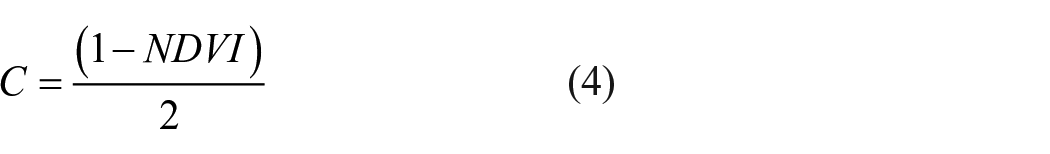
The NDVI-based C factor estimation process, outlined in Figure 2, involved considering Sentinel 2 data of 4 years (168 tiles from January 2019 to December 2022; Cloud cover less than 5%) to calculate the NDVI for the study area. The NDVI was computed and downloaded using GEE platform. For the study, the C factor was calculated from NDVI using the five widely used equations, namely Equation 2 by De Jong et al. (1998), Equation 3 by Van der Knijff et al. (2000), Equation 4 by Durigon et al. (2014), Equation 5 by Wickama et al. (2015) and Equation 6 by Bahrawi et al. (2016). The application of these equations has also been reported by Xiong et al. (2023).

\begin{matrix} C = 0.431 - 0.805 \times N D V I \end{matrix}

(2)

\begin{matrix} C = e^{(\frac{(- 2 \times N D V I)}{(1 - N D V I)})} \end{matrix}

(3)

\begin{matrix} C = \frac{(1 - N D V I)}{2} \end{matrix}

(4)

\begin{matrix} C = 0.227 \times e^{(- 0.997 \times N D V I)} \end{matrix}

(5)

\begin{matrix} C = (0.625 \times N D V I^{2}) - (1.4793 \times N D V I) + 0.8711 \end{matrix}

(6)

Further, an equation was proposed to estimate the C factor from the NDVI pixel value of the NDVI data that were carefully selected to correspond to specific LULC classes within the Netravati Catchment. The selection process ensured that only those NDVI values that accurately represented the respective LULC classes were included in the analysis, allowing each class to exhibit a range of NDVI values that are close but not identical. This approach preserved the natural variability within each LULC class, providing a realistic foundation for further analysis. Waterbodies and Built-up areas were excluded from this selection process due to their distinct spectral characteristics, which were considered outliers and thus not representative of the NDVI – C factor relationship. The regression analysis between NDVI and the C factor was performed and the model was chosen that provided the best fit for the data, capturing the relationship effectively. The Coefficient of Correlation (r), Mean Absolute Error (MAE), Standard Deviation (SD), Root Mean Square Error (RMSE), RMSE observation SD Ratio (RSR) and Kling-Gupta efficiency (KGE) were employed to assess the performance of the results obtained from the NDVI-based equations.

The linear relationship between observed and simulated values is represented by r (Pearson, 1895). A positive perfect correlation equals 1, while no correlation will have a value of 0. MAE is the average absolute difference between actual and predicted values (Chai & Draxler, 2014). RMSE is a critical metric for comparing methods, as it quantifies the discrepancy between model predictions and observed values (Chai & Draxler, 2014). Superior performance is indicated by lower MAE and RMSE, with 0 indicating precise alignment (Moriasi et al., 2007). The RSR standardises RMSE using the observation’s SD, which ranges from 0 to larger positive values. Superior model performance is indicated by a lower RSR (Moriasi et al., 2007). The KGE metric offers a thorough evaluation of model performance, taking into account both precision (bias and variability ratios) and accuracy (correlation coefficient r) (Gupta et al., 2009). A KGE value closer to 1 indicates superior model performance, while lower values indicate inferior performance.

Results and Discussion

This study aims to accurately estimate the C factor for the Netravati catchment using LULC classification and NDVI-based methods, which plays a key role in soil erosion modelling.

Estimation C Factor From LULC map

Level II classification was adopted, and the catchment was classified into 10 classes namely: Built-up, Plantation, Crop, Fallow, Forest, Scrub Forest, Grass/Shrub Land, Barren/Wastelands, River Sand and Water bodies, respectively using RF algorithm. The accuracy assessment was done using 600 (20%) sampling points and a confusion matrix was developed, as shown in Figure 3. An overall accuracy of 93.17% was achieved with a 0.924 Kappa coefficient. The strength of the assessment having a Kappa coefficient within the range of 0.81 to 1 is considered perfect (Abd El-Hamid et al., 2021; Anand et al., 2023). The user’s and producer’s accuracy of each class is also given in Figure 3. The chance that a pixel classified as a specific class genuinely belongs to that class is indicated by the user’s accuracy, while the chance that a specific class is correctly identified is indicated by the producer’s accuracy (Nicolau et al., 2024; Rwanga & Ndambuki, 2017; Sun et al., 2023). Apart from Barren/Wasteland with a producer’s accuracy of 87.27%, all the classes have user’s accuracy and producer’s accuracy >90%, highlighting the effectiveness of the RF algorithm in accurately classifying LULC classes as claimed by Talukdar et al. (2020).

Figure 3.

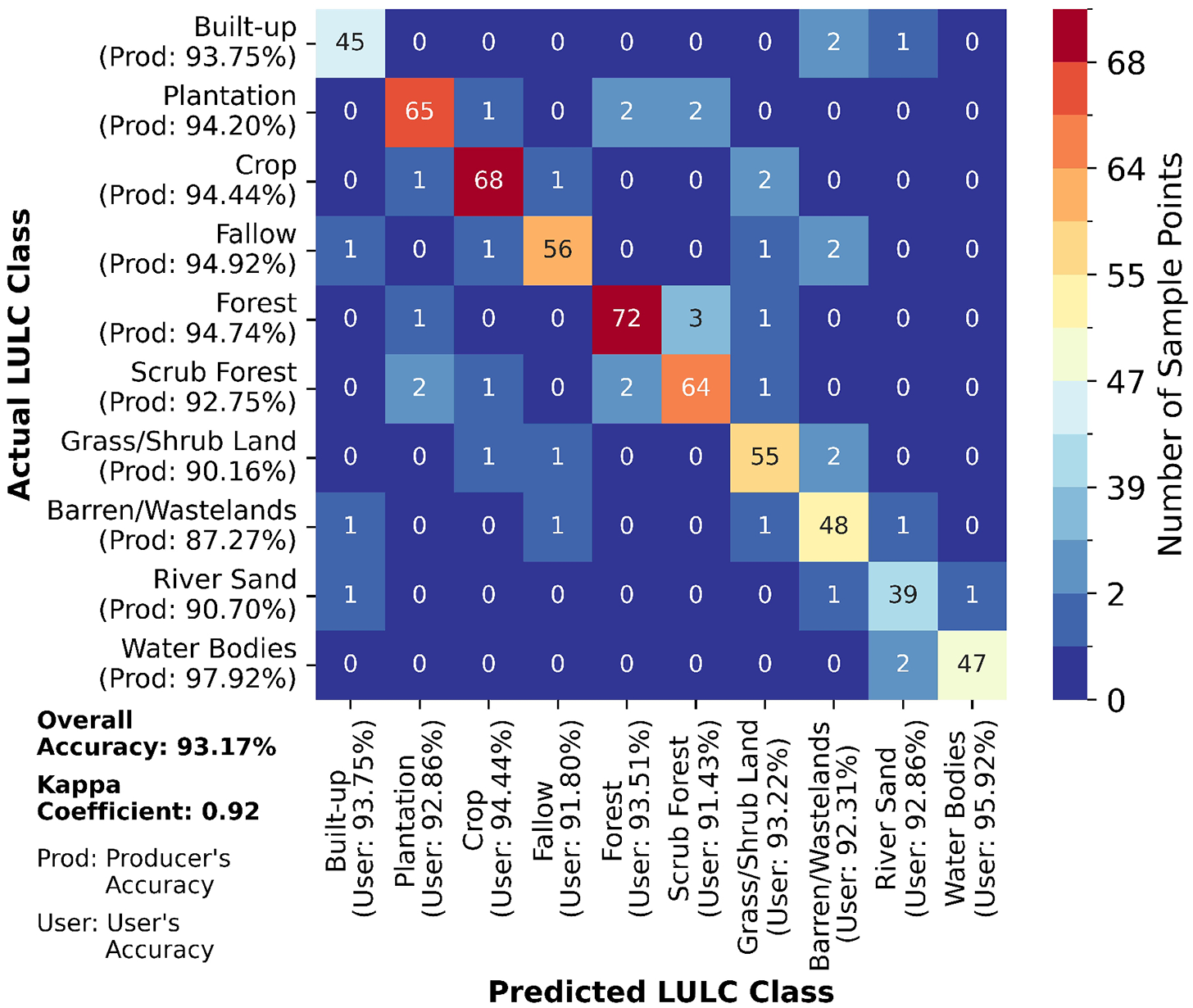
Confusion matrix of RF classified LULC in the Netravati catchment, showing sample counts and class‑wise producer’s and user’s accuracies.

An overview of land distribution within the catchment area was found, highlighting diverse land use patterns (Figure 4(a)). The area distribution in km², and the percentage area, present the spatial extent of various LULC classes as shown in the doughnut plot in Figure 4(b). In the doughnut plot, the LULC classes have been assigned colours corresponding to those in the LULC map. Among all the classes, Forest covers a considerable 1548.10 km² (45.33%), with plantation and Grass/Shrub land also covering sizable areas of 516.29 km² (15.12%) and 378.47 km² (11.08%), respectively. As the terrain towards the western side of the study area is flatter than the eastern side where the ghats are present, agricultural areas (Crops and Plantations) and Built-up areas are predominant, while Forest primarily covers the east side of the study area. This aligns with the findings by Rege et al., (2022) for parts of the Sindhudurg district, also present in Western Ghats.

Figure 4.

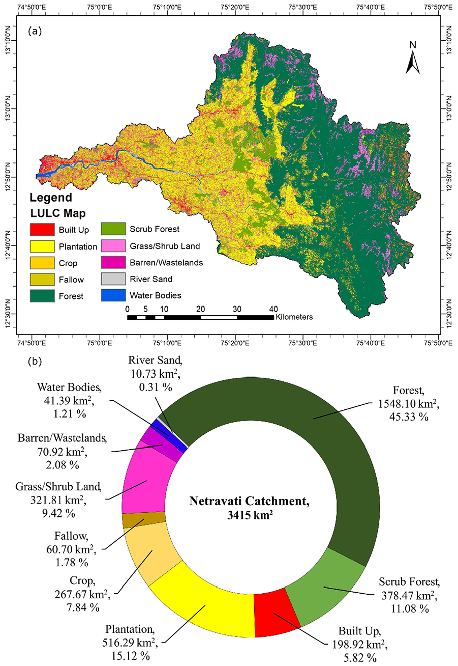
Results of LULC classification in the Netravati catchment: (a) spatial map of 10 LULC classes derived from RF algorithm (b) Doughnut chart quantifying the areal extent and percent share of each class.

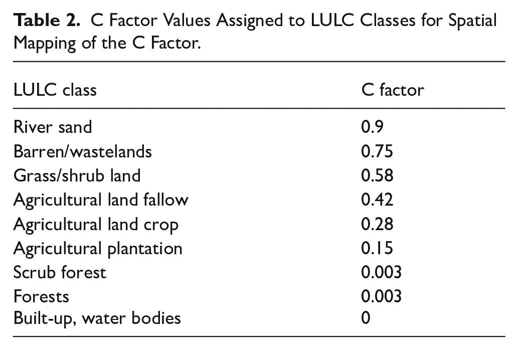
For the computation of the C factor, the LULC classes were assigned the C factor values represented in Table 2 given by ICAR. Several researchers have assigned the C factor in this agroecological region according to their own LULC maps (Ganasri & Ramesh, 2016; Markose & Jayappa, 2016). For the respective LULC classes in the study area, River Sand and Barren/Wastelands, with C factors of 0.9 and 0.75, respectively indicate higher erosion vulnerability due to limited vegetation cover. Grass/Shrubland exhibits a better comparable erosion-resistant with a C factor of 0.58, attributed to its protective plant cover. Fallow Land and Crop have C factors of 0.42 and 0.28, indicating varying degrees of erosion potential. Forests have a low C factor of 0.003, highlighting their ability to mitigate erosion through dense vegetation. Built-up and Waterbodies classes possess the lowest C factor, indicating no soil erosion potential on these surfaces. The C factor map of the catchment was developed based on these attributed values, as shown in Figure 5. The percentage of each erosive C factor value is the same as the corresponding LULC class percentage shown in Figure 4(b).

Table 2.

C Factor Values Assigned to LULC Classes for Spatial Mapping of the C Factor.

LULC class	C factor
River sand	0.9
Barren/wastelands	0.75
Grass/shrub land	0.58
Agricultural land fallow	0.42
Agricultural land crop	0.28
Agricultural plantation	0.15
Scrub forest	0.003
Forests	0.003
Built-up, water bodies	0

Figure 5.

Spatial distribution of C factor across the Netravati catchment prepared from LULC map and corresponding C factor values.

Estimation C Factor From Normalised Difference Vegetation Index (NDVI)

The average NDVI values varied from −0.522 to 0.876 as shown in Figure 6, indicating a wide range of vegetation cover within the Netravati Catchment. This variation in NDVI reflects the heterogeneity of LULC classes present in the region, ranging from waterbodies, bare soil and fallow land to well-established forested and agricultural areas. The spatial variability in NDVI observed also aligns with the LULC map. Regions with higher NDVI values are, therefore supposed to contribute less to erosion because of good vegetation and those with lower NDVI values are more prone to erosion (Ayalew et al., 2020; Guo et al., 2023), thus calling for site-specific conservation efforts in those regions. This further validates the integration of NDVI into the C factor calculation. The C factor was computed from NDVI-based methods (Equation 2 to Equation 6). The Equations 2 and 4, given by De Jong et al. (1998) and Durigon et al. (2014) assume a linear relationship exists between NDVI and the C factor. While Equations 3, 5 and 6, given by Van der Knijff et al. (2000), Wickama et al. (2015), and Bahrawi et al. (2016), respectively assume a nonlinear relationship between NDVI and the C factor. Equation 3 has been utilised by researchers in this agroecological region (Aswathi et al., 2022; Prasannakumar et al., 2011).

Figure 6.

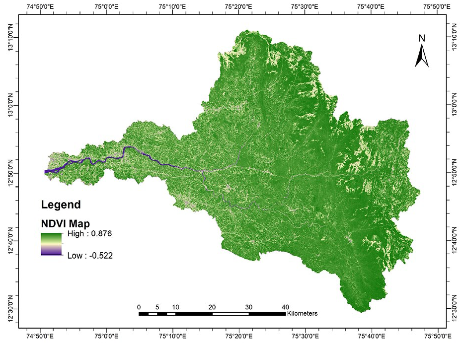
NDVI map of the Netravati catchment derived from Sentinel 2 data, showing vegetation density gradients.

The C factor values derived from these equations ranged from −0.274 to 0.851 for Equation 2 (Figure 7(a)), 0 to 1.986 for Equation 3 (Figure 7(b)), 0.062 to 0.761 for Equation 4 (Figure 7(c)), 0.095 to 0.381 for Equation 5 (Figure 7(d)), and 0.061 to 1.819 for Equation 6 (Figure 7(e)). Comparing these results with the actual C factor values reveals that these equations either overpredict or underpredict the C factor, with some values exceeding the nominal range of 0 to 1. Such C factor values can result in erroneous estimation of soil erosion as also highlighted by Pinson and AuBuchon (2023). This prompted the need to propose a new regional NDVI-based C factor equation. For the development of the equation, exclusion criteria were employed for Built-up areas and Waterbodies. The Built-up area, which gives values similar to those of the Barren area (NDVI approaching 0) and Waterbodies (negative NDVI values) (Saravanan et al., 2019), were not considered due to their limited capacity to generate reliable outcomes. The proposed exponential regression model demonstrated a strong fit to the data, as evidenced by a high R² value of 0.96, indicating that a significant portion of the variability in the C factor was explained by the NDVI values. The regression equation derived for the C factor for the specific region is:

\begin{matrix} C = 2^{(- 5.4 \times N D V I^{2})} \end{matrix}

(7)

This equation captures the non-linear relationship between NDVI and the C factor and is specifically tailored to the conditions of the study region. The C factor values obtained using Equation 7 ranged from 0.056 to 0.99, as shown in Figure 7(f).

Figure 7.

Comparison of C factor spatial estimates based on NDVI using Equations: (a) 2, (b) 3, (c) 4, (d) 5, (e) 6 and (f) 7.

A comparative analysis of different NDVI-based C factor equations and the actual C factor was carried out considering r, MAE, SD, RMSE, RSR and KGE. This comparison was conducted for all LULC classes except Built-up areas and Water bodies, which were considered outliers due to their unique spectral characteristics in the proposed equation. The results are presented in Table 3. In terms of r, most equations show high values around 0.987, except for Wickama et al. (2015) (0.319), which indicates a significant discrepancy in capturing the spatial variability of the C factor. When examining MAE, the proposed equation has the lowest error at 0.048, suggesting it offers the most accurate estimation, whereas other equations like De Jong et al. (1998) (0.370) and Wickama et al. (2015) (0.275) exhibit much higher errors, reflecting less precise estimates. For SD, while the proposed equation shows a value of 0.275, which is higher than most others, this reflects its greater sensitivity to capture local variability. RMSE, another critical measure of error, is notably lowest for the proposed model (0.058), followed by Bahrawi et al. (2016) (0.145), emphasising its robustness in prediction accuracy. Conversely, the Wickama et al. (2015) method (0.350) demonstrates poorer performance. In terms of RSR, a lower value indicates better performance, with the proposed model leading at 0.197, far surpassing other models like (De Jong et al., 1998) (1.329) and Wickama et al. (2015) (1.189), which show substantial errors. The KGE metric, which combines multiple aspects of model performance, highlights the superiority of the proposed equation with a score of 0.921, indicating a near-optimal balance between correlation, bias and variability. Other methods, such as (Bahrawi et al., 2016) (0.552) and Van der Knijff et al. (2000) (0.428), show moderate efficiency, while De Jong et al. (1998) (−0.095) and Wickama et al. (2015) (−0.099) have negative values, signifying poor performance. Based on the statistical measures, the results of proposed Equation 7 are well-aligned with actual observations (Figure 8).

Table 3.

Performance Assessment of the Methods Used for Estimation of C Factor.

Performance indicator	De Jong et al. (1998)	Van der Knijff et al. (2000)	Durigon et al. 2014)	Wickama et al. (2015)	Bahrawi et al. (2016)	Proposed
R	0.987	0.950	0.987	0.319	0.987	0.984
MAE	0.370	0.182	0.182	0.275	0.121	0.048
SD	0.172	0.212	0.107	0.029	0.178	0.275
RMSE	0.391	0.214	0.232	0.350	0.145	0.058
RSR	1.329	0.727	0.789	1.189	0.491	0.197
KGE	-0.095	0.428	0.263	-0.099	0.552	0.921

Figure 8.

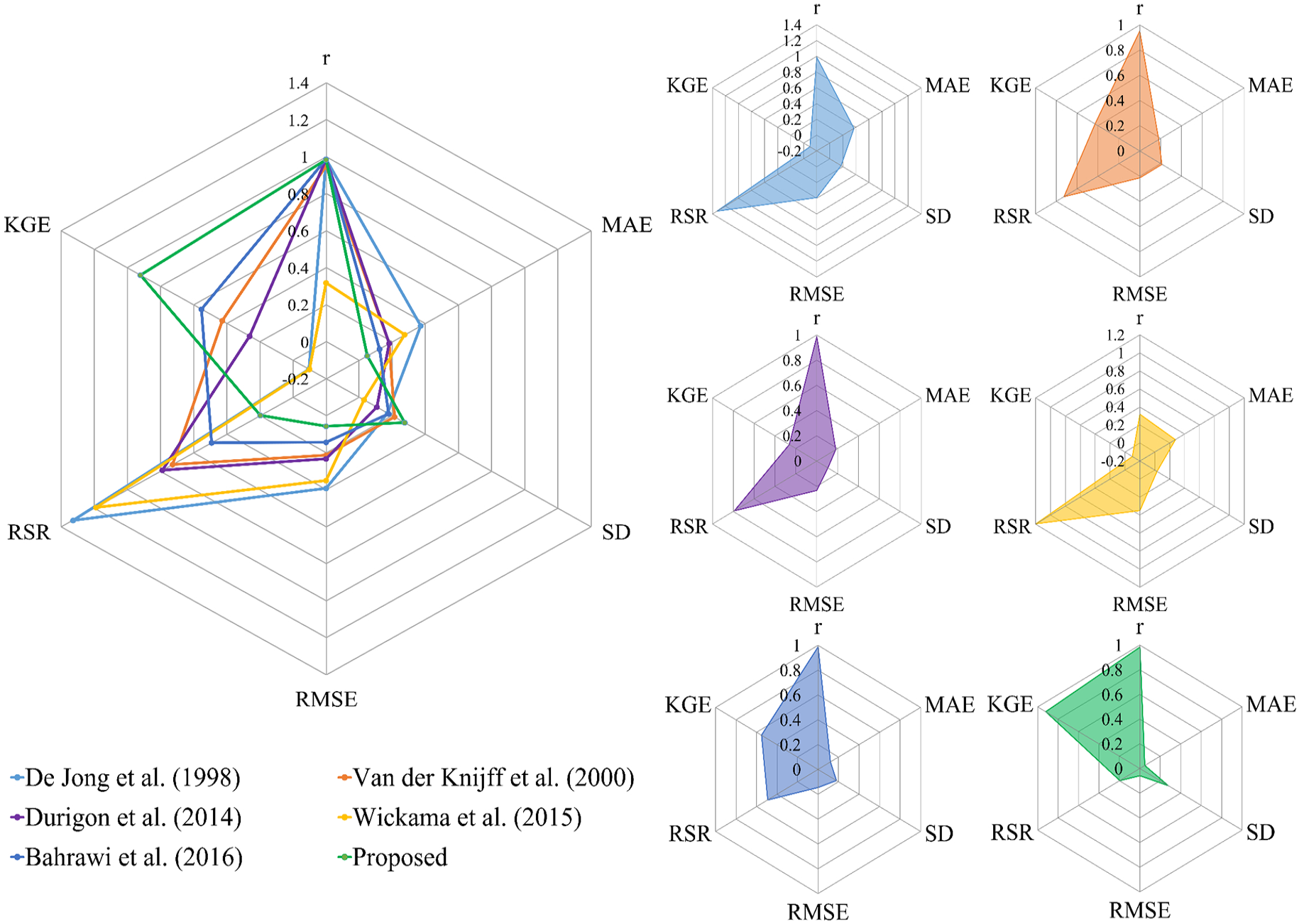
Comparison of different methods to estimate C factor using a radar plot, highlighting relative accuracy and reliability.

The mean and SD for each class (excluding Water and Built-up) from each method are shown in Table 4, enabling a detailed comparison of each method’s performance against the actual C factor values from Table 2. Further, to visualise the variability of the C factor among the LULC classes, boxplots were plotted for De Jong et al. 1998) (Figure 9(a)), Van der Knijff et al. (2000) (Figure 9(b)), Durigon et al. (2014) (Figure 9(c)), Wickama et al. (2015) (Figure 9(d)), Bahrawi et al. (2016) (Figure 9(e)), and proposed Equation 7 (Figure 9(f)). When comparing the C factor values with the actual values, clear deviations are observed, with some methods generating inaccurate negative values, which suggests the failure of those equations in capturing the C factor effectively for this region. Barren/Wastelands, which have an actual C factor value of 0.75, significantly contribute to erosion. The C factor values computed by proposed Equation 7 are well approximated with a value of 0.758 ±. 0.045, followed by (Bahrawi et al., 2016) with a value of 0.522 ± .0.033. Wickama et al. (2015) significantly underestimates the C factor values at 0.173 ± .0.005, as do the other equations. For LULC class Crop having actual C factor 0.28, proposed Equation 7 with value 0.265 ± .0.042 provides a close estimate. Bahrawi et al. 2016) is the next best (0.217 ± .0.026), but values from De Jong et al. (1998) show a negative value (–0.050 ± .0.029) which is inaccurate. For the LULC class Forest Van der Knijff et al. (2000) estimated the C factor values (0.001 ± 0.001), closest to the actual but underestimated C factor value for other LULC classes. The proposed method overestimates slightly at 0.077 ± 0.016, but this is a minor deviation compared to other methods. Similarly, for other LULC classes namely Fallow, Grass/Shrub land, Plantation and River Sand, proposed Equation 7 gives mean values closer to the actual C factor values, whereas other equations show varying degrees of underestimation.

Table 4.

LULC Class-wise Mean and SD of C Factor Values Computed by Different Methods.

Land cover	De Jong et al. (1998)	Van der Knijff et al. (2000)	Durigon et al. (2014)	Wickama et al. (2015)	Bahrawi et al. (2016)	Proposed
Barren/Wastelands	0.213 ± .024	0.475 ± .052	0.364 ± .015	0.173 ± .005	0.522 ± .033	0.758 ± .045
Crop	−0.050 ± .029	0.054 ± .023	0.201 ± .018	0.125 ± .004	0.217 ± .026	0.265 ± .042
Fallow	0.038 ± .028	0.151 ± .039	0.256 ± .018	0.140 ± .005	0.305 ± .031	0.411 ± .052
Forest	−0.202 ± .023	0.001 ± .001	0.107 ± .014	0.104 ± .003	0.101 ± .013	0.077 ± .016
Grass/shrubland	0.129 ± .029	0.303 ± .056	0.313 ± .018	0.156 ± .006	0.411 ± .037	0.591 ± .059
Plantation	−0.136 ± .034	0.011 ± .009	0.148 ± .021	0.113 ± .005	0.146 ± .025	0.158 ± .034
River sand	0.292 ± .010	0.659 ± .023	0.414 ± .006	0.191 ± .002	0.640 ± .015	0.892 ± .014

Figure 9.

Boxplot representing the LULC class-wise comparison of the actual C factor with estimated C factor from Equation: (a) 2, (b) 3, (c) 4, (d) 5, (e) 6 and (f) 7, showing the precision and bias across the LULC classes.

The results show that Wickama et al. (2015) gave the values of the C factor in the range of 0.10 to 0.2 for individual LULC classes. This close range suggests an inability of the method to deal with diverse LULC classes in this region. De Jong et al. (1998) gave negative values for LULC classes Plantation (–0.136 ± .0.034), and Forest (–0.202 ± .0.023) as well, highlighting the failure of this method to compute the C factor for this region. The study by Xiong et al. (2023) stated that global models underestimate C factors at regional scale, aligning with our findings. Similarly, Colman et al. (2018) evaluated Durigon et al. (2014) method and found the equation gave 10 times the C factor values compared to the actual values for the Upper Paraguay Basin located in Brazil and recommended using a multiplying factor of 0.1, which highlights the need for local parameterisation. The proposed Equation 7 consistently provided more precise C factor estimates across the LULC classes present in the study area. This also indicates that regionally parameterised equations are essential for addressing spatial heterogeneity. Additionally, integrating tailored equations can improve erosion estimation, enabling more precise planning of targeted soil conservation efforts like crop rotation and afforestation.

While the proposed NDVI-based equation outperformed other equation in estimating the C factor for the catchment, it is essential to recognise its limitations. The equation is parameterised to the local agroecological conditions, thus restricting its applicability to other agroecological regions. To address this, it is necessary for researchers to calibrate available equations or propose appropriate equations at regional scale. In the study, Built-up and Waterbody classes were considered as spectral outliers due to their reflectance characteristics. The integration of additional RS-derived indices, such as Normalized Difference Built-up Index (NDBI), Normalized Difference Water Index (NDWI), Bare Soil Index (BSI) could enhance the interpretation of spectral characteristics associated with urban surfaces, water bodies and barren land. This could help to capture the LULC dynamics more accurately. Future research can enhance C factor estimation by considering seasonal or monthly scale analysis as done by Allataifeh et al. (2024) and Macedo et al. (2021) and by employing advanced machine learning techniques.

Summary and Conclusions

The study presented a comprehensive approach for parameterising the C factor for the Netravati catchment in the Western Ghats and Coastal Plains region of India. For the study, the LULC and NDVI-based approaches, integrated with the RF algorithm and 10 m high-resolution Sentinel 2 data, were explored for C factor estimation, which proved effective. For the study area, 10 distinct LULC classes were identified, and an overall accuracy of 93.17% was achieved for a detailed LULC map created with a Kappa coefficient of 0.924. The River Sand (10.73 km²), Barren/Wastelands (70.92 km²) and Grass/Shrubland (321.81 km²) are highly vulnerable to erosion due to limited vegetation cover, have C factor of 0.9, 0.75 and 0.52 respectively. Fallow Land (60.70 km²), Crop (267.67 km²) and Plantations (516.29 km²) with lower C factors of 0.42, 0.28 and 0.15 respectively, signifies varying erosion potentials due to their protective vegetation cover. Through the dense vegetation cover, the forest (1926.57 km²) can significantly mitigate erosion and have a C factor of 0.003.

The comparison of previous NDVI-based C factor equations with the actual C factor values revealed significant variation in the results, stressing the importance of regional parameterisation. The proposed region-specific NDVI-based nonlinear equation demonstrated superior performance (R² value of 0.96, r of 0.984, MAE of 0.048, RMSE of 0.058 and KGE of 0.921) compared to other equations representing a near-optimal balance between correlation, bias and variability. The proposed equation gave a mean C factor value close to the actual for distinct LULC types, effectively capturing the variability in the C factor, making it a valuable tool for soil erosion modelling and supporting sustainable land management practices in the region. Although the equation is specific thus limiting its applicability to other regions, the methodology followed in the study can be replicated by researchers elsewhere. Future work could focus on exploring alternative RS-derived indices and machine learning techniques to improve C factor estimation for better soil erosion modelling and mitigation.

Footnotes

Acknowledgements

The authors wish to acknowledge the National Institute of Technology Karnataka, Surathkal for providing the support to carry out the study. We also thank the European Space Agency (ESA) for providing the Sentinel-2 data through the Copernicus program.

ORCID iDs

Waleed Makhdumi

Shwetha H. R.

Jagadeesha B. Pai

Author Contributions

MW, DGS and SHR formulated the methodology. MW did the acquisition of the data and carried out the analysis under the supervision of DGS and SHR. MW drafted the manuscript DGS, SHR and PBJ revised the manuscript and approved this version to be published.

Funding

The author(s) received no financial support for the research, authorship and/or publication of this article.

Declaration of Conflicting Interests

The author(s) declared no potential conflicts of interest with respect to the research, authorship and/or publication of this article.

Data Availability

The primary datasets used and analysed during the current study are freely available online and are available from the corresponding author upon reasonable request.

References

Abd El-Hamid

H. T.

Kaloop

M. R.

Abdalla

E. M.

J. W.

Zarzoura

. (2021). Assessment and prediction of land-use/land-cover change around Blue Nile and White Nile due to flood hazards in Khartoum, Sudan, based on geospatial analysis. Geomatics, Natural Hazards and Risk, 12(1), 1258–1286. https://doi.org/10.1080/19475705.2021.1923577

Alewell

Borrelli

Meusburger

Panagos

(2019). Using the USLE: Chances, challenges and limitations of soil erosion modelling. International Soil and Water Conservation Research, 7(3), 203–225. https://doi.org/10.1016/j.iswcr.2019.05.004

Allataifeh

Rudra

Daggupati

Dhiman

Goel

Prasher

(2024). Spatiotemporal variability in the C-factor: An analysis using high resolution satellite imagery. International Journal of Sediment Research, 39(1), 83–99. https://doi.org/10.1016/j.ijsrc.2023.10.002

Almagro

Thomé

T. C.

Colman

C. B.

Pereira

R. B.

Marcato Junior

Rodrigues

D. B. B.

Oliveira

P. T. S.

(2019). Improving cover and management factor (C-factor) estimation using remote sensing approaches for tropical regions. International Soil and Water Conservation Research, 7(4), 325–334. https://doi.org/10.1016/j.iswcr.2019.08.005

Anand

Rekha

R. S.

Radhakrishnan

Ramaswamy

(2023). Analysis of LULC change dynamics and its impact assessment using CA-ANN model in part of Coimbatore region, India. GeoJournal, 88(6), 5825–5845. https://doi.org/10.1007/s10708-023-10944-0

Aswathi

Sajinkumar

K. S.

Rajaneesh

Oommen

Bouali

E. H.

Binoj Kumar

R. B.

Rani

V. R.

Thomas

Thrivikramji

K. P.

Ajin

R. S.

Abioui

Sajinkumar

K. S.

Ajin

R. S.

Abioui

(2022). Furthering the precision of RUSLE soil erosion with PSInSAR data: An innovative model. Geocarto International, 37, 16108–16131. https://doi.org/10.1080/10106049.2022.2105407

Aulakh

M. S.

Sidhu

G. S.

(2015). Soil degradation in India: Causes, major threats, and management options. In MARCO Symposium 2015 - Next Challenges of Agro-Environmental research in Monsoon Asia (pp. 151–156). National Institute for Agro-Environmental Sciences (NIAES).

Ayalew

D. A.

Deumlich

Šarapatka

Doktor

(2020). Quantifying the sensitivity of NDVI-based C factor estimation and potential soil erosion prediction using spaceborne earth observation data. Remote Sensing, 12(7), 1136. https://doi.org/10.3390/rs12071136

Bagherzadeh

(2014). Estimation of soil losses by USLE model using GIS at Mashhad plain, Northeast of Iran. Arabian Journal of Geosciences, 7(1), 211–220. https://doi.org/10.1007/s12517-012-0730-3

10.

Bahrawi

J. A.

Elhag

Aldhebiani

A. Y.

Galal

H. K.

Hegazy

A. K.

Alghailani

(2016). Soil erosion estimation using remote sensing techniques in Wadi Yalamlam Basin, Saudi Arabia. Advances in Materials Science and Engineering, 2016(1), 9585962. https://doi.org/10.1155/2016/9585962

11.

Belgiu

Drăguţ

(2016). Random forest in remote sensing: A review of applications and future directions. ISPRS Journal of Photogrammetry and Remote Sensing, 114, 24–31. https://doi.org/10.1016/j.isprsjprs.2016.01.011

12.

Benavidez

Jackson

Maxwell

Norton

(2018). A review of the (Revised) Universal Soil Loss Equation ((R)USLE: With a view to increasing its global applicability and improving soil loss estimates. Hydrology and Earth System Sciences, 22, 6059–6086. https://doi.org/10.5194/hess-22-6059-2018

13.

Bera

(2017). Estimation of soil loss by USLE model using GIS and remote sensing techniques: A case study of Muhuri River Basin, Tripura, India. Eurasian Journal of Soil Science, 6(3), 206–206. https://doi.org/10.18393/ejss.288350

14.

Borrelli

Alewell

Alvarez

Anache

J. A. A.

Baartman

Ballabio

Bezak

Biddoccu

Cerdà

Chalise

Chen

De Girolamo

A. M.

Gessesse

G. D.

Deumlich

Diodato

Efthimiou

Erpul

Fiener

. . . Panagos

(2021). Soil erosion modelling: A global review and statistical analysis. Science of the Total Environment, 780, Article 146494. https://doi.org/10.1016/j.scitotenv.2021.146494

15.

Borrelli

Panagos

Langhammer

Apostol

Schütt

(2016). Assessment of the cover changes and the soil loss potential in European forestland: First approach to derive indicators to capture the ecological impacts on soil-related forest ecosystems. Ecological Indicators, 60, 1208–1220. https://doi.org/10.1016/j.ecolind.2015.08.053

16.

Chai

Draxler

R. R.

(2014). Root mean square error (RMSE) or mean absolute error (MAE)? Arguments against avoiding RMSE in the literature. Geoscientific Model Development, 7(3), 1247–1250.

17.

Colman

C. B.

Oliveira

P. T. S.

Almagro

Soares-Filho

(2018). Impacts of climate and land use changes on soil erosion in the Upper Paraguay Basin. Federal University of Mato Grosso Do Sul, Campo Grande.

18.

De Jong

S. M

. (1994). Applications of reflective remote sensing for land degradation studies in a Mediterranean environment. Koninklijk Nederlands Aardrijkskundig Genootschap.

19.

De Jong

S. M.

Brouwer

L. C.

Riezebos

H. T

. (1998). Erosion hazard assessment in the La Peyne catchment, France. Utrecht University.

20.

Durigon

V. L.

Carvalho

D. F.

Antunes

M. A. H.

Oliveira

P. T. S.

Fernandes

M. M.

(2014). NDVI time series for monitoring RUSLE cover management factor in a tropical watershed. International Journal of Remote Sensing, 35(2), 441–453. https://doi.org/10.1080/01431161.2013.871081

21.

Ebabu

Tsunekawa

Haregeweyn

Tsubo

Adgo

Fenta

A. A.

Meshesha

D. T.

Berihun

M. L.

Sultan

Vanmaercke

Panagos

Borrelli

Langendoen

E. J.

Poesen

(2022). Global analysis of cover management and support practice factors that control soil erosion and conservation. International Soil and Water Conservation Research, 10(2), 161–176. https://doi.org/10.1016/j.iswcr.2021.12.002

22.

Felix

K. T.

Ramappa

K. B.

(2023). An economic analysis of crop diversification and dynamics of cropping pattern in Karnataka, India. Humanities and Social Sciences Communications, 10(1), 571. https://doi.org/10.1057/s41599-023-02078-y

23.

Food and Agriculture Organization of United Nations. (2015a). Healthy soils are the basis for healthy food production.

24.

Food and Agriculture Organization of United Nations. (2015b). Status of the world’s soil resources.

25.

Gabriels

Ghekiere

Schiettecatte

Rottiers

(2003). Assessment of USLE cover-management C-factors for 40 crop rotation systems on arable farms in the Kemmelbeek watershed, Belgium. Soil and Tillage Research, 74(1), 47–53.

26.

Ganasri

B. P.

Ramesh

(2016). Assessment of soil erosion by RUSLE model using remote sensing and GIS: A case study of Nethravathi Basin. Geoscience Frontiers, 7(6), 953–961. https://doi.org/10.1016/j.gsf.2015.10.007

27.

Ghosal

Das Bhattacharya

(2020). A review of RUSLE model. Journal of the Indian Society of Remote Sensing, 48(4), 689–707. https://doi.org/10.1007/s12524-019-01097-0

28.

Guo

Pan

Kuai

Dai

Zhu

Jia

Zeng

Lin

(2023). A more accurate approach to estimate the C-factor of RUSLE by coupling stratified vegetation cover index in southern China. Forest Ecology and Management, 541, Article 120979. https://doi.org/10.1016/j.foreco.2023.120979

29.

Gupta

H. V

Kling

Yilmaz

K. K.

Martinez

G. F.

(2009). Decomposition of the mean squared error and NSE performance criteria: Implications for improving hydrological modelling. Journal of Hydrology, 377(1–2), 80–91.

30.

Huang

Wang

K.-R.

Zou

Cao

X.-C.

(2021). Development of global soil erosion research at the watershed scale: A bibliometric analysis of the past decade. Environmental Science and Pollution Research, 28(10), 12232–12244. https://doi.org/10.1007/s11356-020-11888-5

31.

Indraja

Aashi

Vema

V. K.

(2024). Spatial and temporal classification and prediction of LULC in Brahmani and Baitarni basin using integrated cellular automata models. Environmental Monitoring and Assessment, 196(2), 117. https://doi.org/10.1007/s10661-023-12289-0

32.

Iranzad

Liu

(2024). A review of random forest-based feature selection methods for data science education and applications. International Journal of Data Science and Analytics. Advance online publication. https://doi.org/10.1007/s41060-024-00509-w

33.

Jose

D. M.

Vincent

A. M.

Dwarakish

G. S.

(2022). Improving multiple model ensemble predictions of daily precipitation and temperature through machine learning techniques. Scientific Reports, 12(1), 4678. https://doi.org/10.1038/s41598-022-08786-w

34.

Kashiwar

S. R.

Kundu

M. C.

Dongarwar

U. R.

(2022). Soil erosion estimation of Bhandara region of Maharashtra, India, by integrated use of RUSLE, remote sensing, and GIS. Natural Hazards, 110(2), 937–959. https://doi.org/10.1007/s11069-021-04974-5

35.

Ketema

Dwarakish

G. S.

(2021). Water erosion assessment methods: A review. ISH Journal of Hydraulic Engineering, 27(4), 434–441. https://doi.org/10.1080/09715010.2019.1567398

36.

Krasa

Dostal

Vrana

Plocek

(2010). Predicting spatial patterns of sediment delivery and impacts of land-use scenarios on sediment transport in Czech catchments. Land Degradation & Development, 21(4), 367–375.

37.

Lal

(2001). Soil degradation by erosion. Land Degradation & Development, 12(6), 519–539. https://doi.org/10.1002/ldr.472

38.

Lal

(2003). Soil erosion and the global carbon budget. Environment International, 29(4), 437–450. https://doi.org/10.1016/S0160-4120(02)00192-7

39.

Latocha

Szymanowski

Jeziorska

Stec

Roszczewska

(2016). Effects of land abandonment and climate change on soil erosion: An example from depopulated agricultural lands in the Sudetes Mts., SW Poland. Catena, 145, 128–141.

40.

Lee

Ahn

(2017). Estimation of soil erosion rate in the Democratic People’s Republic of Korea using the RUSLE model. Forest Science and Technology, 13(3), 100–108.

41.

Leh

Bajwa

Chaubey

(2013). Impact of land use change on erosion risk: AN integrated remote sensing, geographic information system and modeling methodology. Land Degradation & Development, 24(5), 409–421. https://doi.org/10.1002/ldr.1137

42.

Valladares

G. S.

Batistella

A. M.

(2004). Mapping soil Erosion risk in Rodonia, Brazilian Amazonia: Using RUSLE, remote sensing and GIS. Land Degradation & Development, 15, 499–512. https://doi.org/10.1002/ldr.634

43.

Prosser

I. P.

Moran

C. J.

Gallant

J. C.

Priestley

Stevenson

J. G.

(2003). Predicting sheetwash and rill erosion over the Australian continent. Soil Research, 41(6), 1037–1062.

44.

Macedo

P. M. S.

Oliveira

P. T. S.

Antunes

M. A. H.

Durigon

V. L.

Fidalgo

E. C. C.

de Carvalho

D. F.

(2021). New approach for obtaining the C-factor of RUSLE considering the seasonal effect of rainfalls on vegetation cover. International Soil and Water Conservation Research, 9(2), 207–216. https://doi.org/10.1016/j.iswcr.2020.12.001

45.

Majhi

Shaw

Mallick

Patel

P. P.

(2021). Towards improved USLE-based soil erosion modelling in India: A review of prevalent pitfalls and implementation of exemplar methods. Earth-Science Reviews, 221, Article 103786. https://doi.org/10.1016/j.earscirev.2021.103786

46.

Makhdumi

Dwarakish

G. S.

(2019, June 27). Prioritisation of watersheds using TOPSIS and VIKOR method [Conference session]. Seventh International Conference on Remote Sensing and Geoinformation of the Environment (RSCy2019), Paphos, Cyprus (p. 6). https://doi.org/10.1117/12.2532024

47.

Makhdumi

Shwetha

H. R.

Dwarakish

G. S.

(2023). Soil erosion in diverse agroecological regions of India: A comprehensive review of USLE-based modelling. Environmental Monitoring and Assessment, 195(9), 1112. https://doi.org/10.1007/s10661-023-11687-8

48.

Markose

V. J.

Jayappa

K. S.

(2016). Soil loss estimation and prioritization of sub-watersheds of Kali River basin, Karnataka, India, using RUSLE and GIS. Environmental Monitoring and Assessment, 188(4), 225. https://doi.org/10.1007/s10661-016-5218-2

49.

Martínez-Mena

Carrillo-López

Boix-Fayos

Almagro

Franco

N. G.

Díaz-Pereira

Montoya

De Vente

(2020). Long-term effectiveness of sustainable land management practices to control runoff, soil erosion, and nutrient loss and the role of rainfall intensity in Mediterranean rainfed agroecosystems. Catena, 187, Article 104352.

50.

McClarren

R. G.

(2021). Decision trees and random forests for regression and classification. In R. G.

McClarren

(Ed.), Machine learning for engineers: Using data to solve problems for physical systems (pp. 55–82). Springer International Publishing. https://doi.org/10.1007/978-3-030-70388-2_3

51.

Mohammed

J. A.

Gashaw

Yimam

Z. A.

(2025). Identification of erosion-prone watersheds for prioritizing soil and water conservation in a changing climate using morphometric analysis and GIS. Natural Hazards, 121(4), 4171–4189. https://doi.org/10.1007/s11069-024-06952-z

52.

Moriasi

D. N.

Arnold

J. G.

Van Liew

M. W.

Bingner

R. L.

Harmel

R. D.

Veith

T. L.

(2007). Model evaluation guidelines for systematic quantification of accuracy in watershed simulations. Transactions of the ASABE, 50(3), 885–900.

53.

Mukharamova

Saveliev

Ivanov

Gafurov

Yermolaev

(2021). Estimating the soil Erosion cover-management factor at the european part of Russia. ISPRS International Journal of Geo-Information, 10(10), 645. https://doi.org/10.3390/ijgi10100645

54.

National Remote Sensing Centre. (2019). Status of land degradation in India: 2015-16. National Remote Sensing Centre, ISRO.

55.

Nearing

M. A.

Jetten

Baffaut

Cerdan

Couturier

Hernandez

Le Bissonnais

Nichols

M. H.

Nunes

J. P.

Renschler

C. S.

Souchère

Van Oost

(2005). Modeling response of soil erosion and runoff to changes in precipitation and cover. Catena, 61(2–3), 131–154. https://doi.org/10.1016/j.catena.2005.03.007

56.

Nearing

M. A.

Lane

L. J.

Lopes

V. L.

(1994). Modeling soil erosion. In By Soil and Water Conservation Society (U. S.) & Lal

(Eds.), Soil erosion research methods (pp. 127–158). Routledge.

57.

Nicolau

A. P.

Dyson

Saah

Clinton

(2024). Accuracy assessment: Quantifying classification quality. In J. A.

Cardille

M. A.

Crowley

Saah

N. E

Clinton

(Eds.), Cloud-based remote sensing with Google earth engine: Fundamentals and applications (pp. 135–145). Springer International Publishing. https://doi.org/10.1007/978-3-031-26588-4_7

58.

Pal

D. K.

(2019). Agro-ecological regions for better crop planning and ecosystem services. In Pal

D. K.

(Ed.), Ecosystem services and tropical soils of India (pp. 7–27). Springer International Publishing. https://doi.org/10.1007/978-3-030-22711-1_2

59.

Panagos

Ballabio

Poesen

Lugato

Scarpa

Montanarella

Borrelli

(2020). A soil erosion indicator for supporting agricultural, environmental and climate policies in the European union. Remote Sensing, 12(9), 1365. https://doi.org/10.3390/RS12091365

60.

Panagos

Borrelli

Meusburger

Alewell

Lugato

Montanarella

(2015). Estimating the soil erosion cover-management factor at the European scale. Land Use Policy, 48, 38–50. https://doi.org/10.1016/j.landusepol.2015.05.021

61.

Parsons

A. J.

(2019). How reliable are our methods for estimating soil erosion by water? Science of The Total Environment, 676, 215–221. https://doi.org/10.1016/j.scitotenv.2019.04.307

62.

Pásztor

Waltner

Centeri

Belényesi

Takács

(2016). Soil erosion of Hungary assessed by spatially explicit modelling. Journal of Maps, 12(sup1), 407–414.

63.

Paul

Majumder

Ghosh

(2024). Exploring the LULC dynamics and its relation with land surface temperature variation using split window algorithm: A study of Barasat subdivision, West Bengal, India. Environmental Monitoring and Assessment, 196(11), 1070. https://doi.org/10.1007/s10661-024-13180-2

64.

Pearson

(1895). VII. Note on regression and inheritance in the case of two parents. Proceedings of The Royal Society of London, 58(347–352), 240–242.

65.

Pham

T. N.

Yang

Kanae

Oki

Musiake

(2001). Application of RUSLE model on global soil erosion estimate. Proceedings of Hydraulic Engineering, 45, 811–816.

66.

Pinson

A. O.

AuBuchon

J. S.

(2023). A new method for calculating C factor when projecting future soil loss using the Revised Universal soil loss equation (RUSLE) in semi-arid environments. CATENA, 226, Article 107067. https://doi.org/10.1016/j.catena.2023.107067

67.

Prasannakumar

Shiny

Geetha

Vijith

(2011). Spatial prediction of soil erosion risk by remote sensing, GIS and RUSLE approach: A case study of Siruvani river watershed in Attapady valley, Kerala, India. Environmental Earth Sciences, 64(4), 965–972. https://doi.org/10.1007/s12665-011-0913-3

68.

Rawat

K. S.

Singh

S. K.

(2018). Appraisal of soil conservation capacity using NDVI model-based C factor of RUSLE model for a semi arid ungauged watershed: A case study. Water Conservation Science and Engineering, 3(1), 47–58. https://doi.org/10.1007/s41101-018-0042-x

69.

Rege

Warnekar

S. B.

Lee

J. S. H.

(2022). Mapping cashew monocultures in the Western Ghats using optical and radar imagery in Google Earth Engine. Remote Sensing Applications: Society and Environment, 28, Article 100861. https://doi.org/10.1016/j.rsase.2022.100861

70.

Renard

K. G.

Foster

G. R.

Weesies

G. A.

McCool

D. K.

Yoder

D. C.

(Eds.) (1997). Predicting soil Erosion by water: A guide to conservation planning with the revised universal soil loss equation (RUSLE). In USDA agriculture handbook No. 703 (p. 404). https://doi.org/DC0-16-048938-565–100

71.

Richi

S. M.

(2025). Integrated RUSLE-GIS modeling for enhancing soil erosion management in Ghamima River Basin, Syria. DYSONA - Applied Science, 6(1), 104–112. https://doi.org/10.30493/das.2024.479955

72.

Rodriguez-Galiano

V. F.

Ghimire

Rogan

Chica-Olmo

Rigol-Sanchez

J. P.

(2012). An assessment of the effectiveness of a random forest classifier for land-cover classification. ISPRS Journal of Photogrammetry and Remote Sensing, 67, 93–104. https://doi.org/10.1016/j.isprsjprs.2011.11.002

73.

Rwanga

S. S.

Ndambuki

J. M.

(2017). Accuracy assessment of land use/land cover classification using remote sensing and GIS. International Journal of Geosciences, 8(4), 611.

74.

Sampath

V. K.

Radhakrishnan

(2023). A comparative study of LULC classifiers for analysing the cover management factor and support practice factor in RUSLE model. Earth Science Informatics, 16(1), 733–751. https://doi.org/10.1007/s12145-022-00911-7

75.

Sankalpa

J. K. S.

Rathnayaka

A. M. R. W. S. D.

Ishani

P. G. N.

Liyanaarachchi

L. A. T. S.

Gayan

M. W. H.

Wijesuriya

Karunaratne

(2024). Fusion of spectral and topographic features for land use mapping using a machine learning framework for a regional scale application. Environmental Monitoring and Assessment, 196(11), 1030. https://doi.org/10.1007/s10661-024-13178-w

76.

Santra

Mitra

S. S.

(2020). Space-Time Drought Dynamics and Soil Erosion in Puruliya District of West Bengal, India: A Conceptual Design. Journal of the Indian Society of Remote Sensing, 48(8), 1191–1205. https://doi.org/10.1007/s12524-020-01147-y

77.

Saravanan

Jegankumar

Selvaraj

Jacinth Jennifer

Parthasarathy

K. S. S.

(2019). Utility of landsat data for assessing mangrove degradation in Muthupet Lagoon, South India. In Mu

Ramkumar

R. A

James

Menier

Kumaraswamy

(Eds.), Coastal zone management (pp. 471–484). Elsevier. https://doi.org/10.1016/B978-0-12-814350-6.00020-3

78.

Singha

Choudhary

Vishnu

(2014). Growth and diversification of horticulture crops in Karnataka: An inter-district analysis. Sage Open, 4(3), 2158244014548018. https://doi.org/10.1177/2158244014548018

79.

Space Application Centre. (2016). Desertification and Land Degradation Atlas of India (Based on IRS AWiFS data of 2011-13 and 2003-05). Space Application Centre, ISRO.

80.

Sun

Jian

Zhao

Chen

(2023). Species classification and carbon stock assessment of Mangroves in Qi’ao Island with worldview-3 imagery. Forests, 14(12), 1–17. https://doi.org/10.3390/f14122356

81.

Talukdar

Singha

Mahato

Shahfahad, Pal

Liou

Y.-A.

Rahman

(2020). Land-use land-cover classification by machine learning classifiers for satellite observations: A review. Remote Sensing, 12(7), 1135. https://doi.org/10.3390/rs12071135

82.

Taye

Vanmaercke

Poesen

Van Wesemael

Tesfaye

Teka

Nyssen

Deckers

Haregeweyn

(2018). Determining RUSLE P- and C-factors for stone bunds and trenches in rangeland and cropland, North Ethiopia. Land Degradation & Development, 29(3), 812–824. https://doi.org/10.1002/ldr.2814

83.

Teng

Liang

Chen

Liu

Rossel

R. A. V.

Chappell

Shi

(2018). Current and future assessments of soil erosion by water on the Tibetan Plateau based on RUSLE and CMIP5 climate models. Science of the Total Environment, 635, 673–686.

84.

Teng

Viscarra Rossel

R. A.

Shi

Behrens

Chappell

Bui

(2016). Assimilating satellite imagery and visible–near infrared spectroscopy to model and map soil loss by water erosion in Australia. Environmental Modelling & Software, 77, 156–167. https://doi.org/10.1016/j.envsoft.2015.11.024

85.

Thomas

Joseph

Thrivikramji

K. P.

(2018). Assessment of soil erosion in a monsoon-dominated mountain river basin in India using RUSLE-SDR and AHP. Hydrological Sciences Journal, 63(4), 542–560. https://doi.org/10.1080/02626667.2018.1429614

86.

Van der Knijff

J. M. F.

Jones

R. J. A.

Montanarella

. (2000). Soil erosion risk assessment in Europe. European Soil Bureau, European Commission Brussels.

87.

Vereecken

Schnepf

Hopmans

J. W.

Javaux

Roose

Vanderborght

Young

M. H.

Amelung

Aitkenhead

Allison

S. D.

Assouline

Baveye

Berli

Brüggemann

Finke

Flury

Gaiser

Govers

. . . Young

I. M.

(2016). Modeling soil processes: Review, key challenges, and new perspectives. Vadose Zone Journal, 15(5), 1–57. https://doi.org/10.2136/vzj2015.09.0131

88.

Waltner

Saeidi

Grósz

Centeri

Laborczi

Pásztor

(2020). Spatial assessment of the effects of land cover change on soil erosion in Hungary from 1990 to 2018. ISPRS International Journal of Geo-Information, 9(11), 667.

89.

Wickama

Masselink

Sterk

(2015). The effectiveness of soil conservation measures at a landscape scale in the West Usambara highlands, Tanzania. Geoderma, 241–242, 168–179. https://doi.org/10.1016/j.geoderma.2014.11.020

90.

Wischmeier

W. H.

Smith

D. D.

(1978). Predicting rainfall erosion losses. A guide to conservation planning. In USDA-ARS handbook No. 282 (pp. 1–58). https://doi.org/10.1029/TR039i002p00285

91.

Xiong

Leng

Tang

(2023). Global analysis of the cover-management factor for soil Erosion modeling. Remote Sensing, 15(11), 2868. https://doi.org/10.3390/rs15112868

92.

Yang

Kanae

Oki

Koike

Musiake

(2003). Global potential soil erosion with reference to land use and climate changes. Hydrological Processes, 17(14), 2913–2928.

93.

Yang

Zhang

Yin

Zhang

Zhu

Liu

(2020). Remote sensing estimation of the soil erosion cover-management factor for China’s Loess Plateau. Land Degradation & Development, 31(15), 1942–1955. https://doi.org/10.1002/ldr.3577

94.

Yesuph

A. Y.

Dagnew

A. B.

(2019). Soil erosion mapping and severity analysis based on RUSLE model and local perception in the Beshillo Catchment of the Blue Nile Basin, Ethiopia. Environmental Systems Research, 8(1), 17. https://doi.org/10.1186/s40068-019-0145-1

95.

Zhang

Liu

Qiao

(2011, June 24–26). Estimation of the USLE cover and management factor C using satellite remote sensing: A review [Conference session]. 2011 19th International Conference on Geoinformatics, Shanghai, China (pp. 1–5). https://doi.org/10.1109/GeoInformatics.2011.5980735

96.

Zhao

Zhu

Cao

Zha

Myneni

R. B.

(2024). A global dataset of the fraction of absorbed photosynthetically active radiation for 1982–2022. Scientific Data, 11(1), 707. https://doi.org/10.1038/s41597-024-03561-0

Addressing Spatial Variability in Estimating Cover Management Factor of Soil Erosion Models using Geoinformatics: A Case Study of Netravati Catchment,Karnataka,India

Abstract

Keywords

Introduction

Study Area

Materials and Methodology

Datasets

Estimation of C factor from LULC classification

Estimation of C factor from Normalised Difference Vegetation Index (NDVI)

Results and Discussion

Estimation C Factor From LULC map

Estimation C Factor From Normalised Difference Vegetation Index (NDVI)

Summary and Conclusions

Footnotes

Acknowledgements

ORCID iDs

Author Contributions

Funding

Declaration of Conflicting Interests

Data Availability

References