Sage Journals: Discover world-class research

Abstract

Lakes are essential to global freshwater systems, supporting ecosystem services and ecological processes, but they are increasingly impacted by climate change and human activities. This study examined the long-term dynamics of Lakes Abaya and Chamo in the Ethiopian Rift Valley using Landsat images, altimetry-derived lake level data, and a machine learning method within Google Earth Engine, specifically a Multi-Index-based Random Forest (MIRF) classifier. The MIRF classifier achieved high accuracy, ranging from 97.58% to 99.13%, in extracting lake surface water. Substantial fluctuations in lake areas and lake levels were observed: Lake Abaya’s area decreased from 2000 to 2005 at a rate of 6.67 km²/year, then expanded until 2022 at the same increasing rate; Lake Chamo’s area decreased from 2000 to 2010 at a rate of 1.62 km²/year, then expanded until 2022 at a rate of 2.88 km²/year. The correlation analysis between lake areas and environmental factors such as Rainfall (RF), Temperature (TEMP), Normalized Difference Vegetation Index (NDVI), Groundwater Storage (GWS), Terrestrial Water Storage (TWS), and Soil Moisture (SM) revealed important associations. For Lake Abaya, strong correlations were identified with NDVI and TWS, suggesting that vegetation cover and terrestrial water significantly influence its area changes. In contrast, for Lake Chamo, NDVI emerged as the key driver, indicating that vegetation dynamics play a crucial role in the lake’s fluctuations. Furthermore, higher-order polynomial regression models were developed to better capture the complex relationships between lake area and water levels for both lakes. In general, this study integrates remote sensing, machine learning, and cloud computing, offering valuable insights into the lakes’ long-term characteristic and providing critical information for future water resource management strategies.

Keywords

Lake Abaya and Chamo Ethiopia East African rift valley Google Earth Engine Random Forest lake water dynamics Landsat image remote sensing

Introduction

Lakes, as essential components of the Earth’s fresh surface water resources, play a crucial role in providing significant ecosystem services, including water supply, biodiversity support, and climate regulation (Huang et al., 2023; Yue et al., 2023). They also contribute to hydrological and ecological cycles, helping to maintain regional environmental balance (Yilmaz, 2023). However, due to ongoing adverse climate changes and substantial human interventions, the spatial and temporal distribution of lake water has undergone profound changes (Tercan & Atasever, 2021; Yue et al., 2023). This makes it imperative to conduct comprehensive studies on lake dynamics and their driving factors. The geography, geology, and hydrodynamics of lake basins significantly influence these changes. For example, sediment transport due to erosion-prone landscapes and changes in groundwater inflow/outflow due to geological characteristics are key elements that shape the hydrodynamics of lakes, ultimately affecting lake area and water volume. Understanding these processes is crucial for ensuring the sustainable management of lakes and the long-term resilience of their ecosystems.

Given the complex interplay between these factors, precise and continuous monitoring of spatial and temporal changes in surface water is essential (Abujayyab et al., 2021). Remote sensing has become a widely used tool for this purpose because it provides frequent, reliable, and easy-to-access data on lake water dynamics (Wei et al., 2020). Numerous remote sensing satellites, including Landsat (Lu et al., 2020; Yilmaz, 2023), Sentinel-2 (Yang et al., 2020), Sentinel-1 (Jiang et al., 2021; J. Wang et al., 2023), and a combination of optical (Landsat or Srntinel-2) and Sentinel-1 (Dervisoglu, 2022; Tang et al., 2022) have been employed for lake water monitoring. The Sentinel-1, a Synthetic Aperture Radar (SAR) satellite, is particularly advantageous due to its ability to penetrate cloud cover and provide high-resolution images of water surfaces under all weather conditions (Dong et al., 2021; Gómez Fernández et al., 2022; Jiang et al., 2021). While Sentinel-2 provides high-resolution optical imagery for cloud-free periods, both Sentinel-1 and Sentinel-2 are limited by their relatively short record of data, as they have only been operational for the last decade. In contrast, Landsat satellites, with a history dating back to the 1970s and a 16-day revisit period, provide an excellent option for long-term monitoring of lake water dynamics due to their extensive time series and global coverage (X. Li et al., 2019).

Satellite images, owing to their large data size, pose challenges for conventional methods in handling and analyzing data for wide spatial extents and longer time series. Consequently, a cloud computing platform, Google Earth Engine (GEE), has been introduced by Google to address these challenges. GEE provides satellite images, reanalysis products, and robust computing infrastructure (R. G. Xu et al., 2019). Numerous studies have successfully applied GEE in surface water resources studies (Albarqouni et al., 2022; Arora et al., 2023; F. Chen et al., 2017; Jiang et al., 2021; Kandekar et al., 2021; K. Li et al., 2022; Sodhi et al., 2024; Tang et al., 2022; Xia et al., 2019; R. G. Xu et al., 2019). For instance, mapping glacial lakes (F. Chen et al., 2017), estimating lake surface water temperature (Albarqouni et al., 2022), and monitoring lake surface area dynamics (Jiang et al., 2021). GEE’s ability to integrate multi-source data and its capacity to process time series from multiple satellite sensors make it particularly useful for long-term monitoring of lake systems.

In extracting water surfaces from images, determining threshold values is a time-consuming and challenging task for long time series images, due to inter-class resemblance between water and non-water classes that can lead to misclassification (Dehkordi et al., 2022; Kebede et al., 2020). Many index-based studies such as Dervisoglu (2022) resort to using affixed threshold value. Alternatively, automatic thresholding algorithms, such as Otsu’s algorithm, are widely used to determine threshold values based on the histogram of grayscale or single-band images (Yilmaz, 2023). For instance, Jiang et al. (2021) applied Otsu’s algorithm to create an automatic water extraction framework for lake monitoring. Similarly, Asfaw et al. (2020) employed Otsu’s method to extract the lake water area of Lake Ziway, Ethiopia, from 2009 to 2018 using spectral indices from Landsat ETM+ and OLI images. Additionally, some studies have employed multiple indices in combination to reduce misclassifications, although this approach is prone to subjectivity (R. Wang et al., 2020; B. Zhao, 2019; Zhou et al., 2019). However, Machine Learning (ML) techniques have emerged as powerful tools for classification, with Random Forest (RF), Support Vector Machine (SVM), and Classification and Regression Tree (CART) being widely applied (Gómez Fernández et al., 2022; C. Wang et al., 2018). These ML methods are built-in functions within the GEE platform, providing higher accuracy compared to thresholding methods (Kandekar et al., 2021; Noi Phan et al., 2020).

Besides evaluating lake water surface dynamics, it is imperative to investigate the factors driving to these changes. Factors such as climate change (Y. Li et al., 2021; VanDeWeghe et al., 2022), human interventions (Gebrehiwot et al., 2022), changes in land use/land cover, and extreme weather events (Havens et al., 2016) are identified as influential elements in the dynamism of lake water. These factors can be broadly categorized into climatic, environmental, and anthropogenic aspects. Within the climatic factors, precipitation and temperature are particularly noteworthy in shaping changes in lake area and influencing hydrological dynamics across contributing basins (X. Li et al., 2019). Hydrological variables for lake area changes are directly or indirectly dependent on climate-related factors such as basin soil moisture, groundwater storage (Vasilevskiy et al., 2022), and terrestrial water storage (Khorrami et al., 2023; Richey et al., 2015). Likewise, the Vegetation status of contributing basins is an environmental factor highly influencing lake water changes. A commonly adopted method has been used to examine the vegetation status of a given basin evaluating the time series Normalized Difference Vegetation Index.

This study aims to assess the time series lake area dynamics of Lakes Abaya and Chamo using Landsat images from 2000 to 2022. The study will employ a multi-index-based Random Forest (RF) classifier within the GEE cloud computing platform to analyze lake area changes and model the relationship between lake area and lake-level data. Furthermore, it will investigate the climatic and environmental factors influencing lake water fluctuations, contributing to better management and conservation of these vital water resources.

Study Area

The study area encompasses the Abaya and Chamo lakes, and the basin at large, a region of ecological and hydrological significance located in the southern portion of the Rift Valley of Ethiopia. Lake Abaya-Chamo basin is geographically bounded with 37°14′58.57″ to 38°38′38.02″ longitude and 5°25′1.2″ to 8°6′37.68″ latitude (Figure 1).

Figure 1.

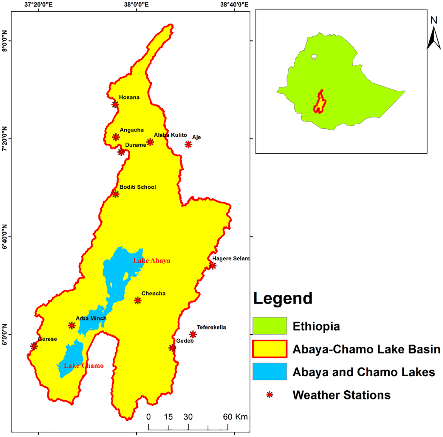
A map showing location and elevation of the Study area (Abaya-Chamo lake basin).

The basin exhibits a unique combination of geographical, climatic, and anthropogenic factors that influence the hydrology and ecological balance of the lakes. The region is also known for its varying tectonic activity (Bewketu, 2015; Daniel et al., 2019), and experiences a semi-arid to sub-humid climate, with distinct wet and dry seasons. Climatic variations, together with land use changes, have implications for the water levels, surface area, water quality, and overall sustainability of the lakes in the basin (Dervisoglu, 2022; Temesgen et al., 2022).

The hydro-ecological significance of the Abaya-Chamo Lake basin extends beyond its immediate vicinity. The lakes and their surrounding basin support a diverse array of flora and fauna. Additionally, the lakes play a crucial role in local agriculture, providing water f or irrigation and influencing the microclimate of the surrounding areas.

Data and Data Sources

This study emphasized on long term analysis of annual fluctuation in the surface area of Lake Abaya and Lake Chamo from the year 2000 to 2022 employing Landsat images. This investigation aimed at elucidating the causal factors inducing the fluctuations in the lake areas, with a careful examination of satellite, reanalysis and hydro-meteorological variables obtained from GEE and station-based observations. The factors responsible for the lake area fluctuation were assessed using satellite reanalysis and station-based hydro-meteorological variables. The following section describes the necessary data elements essential for the execution of this study.

Landsat 5, Landsat 7ETM+, and Landsat 8

From the GEE cloud computing and archiving platform Landsat 5, Landsat 7ETM+, and Landsat 8 OLI imageries were obtained for the Lakes Abaya and Chamo region. These Landsat images have a spatial resolution of 30 m and a 16-day revisit time. About 372 images were filtered based on specified filtering criteria such as cloud cover percentage and region of interest, spanning from 2000 to 2022.

Altimeter-derived lake level data

Lake level data for Abaya and Chamo lakes were collected from two online databases, as well as from the Ministry of Water Resources of Ethiopia, for validation purposes. The two databases used are the Global Reservoir and Lake Monitor (G-REALM) and the Database for Hydrological Time Series of Inland Waters (DAHITI). Both G-REALM and DAHITI provide satellite radar altimeter-derived surface water level data for lakes and reservoirs (K. Li et al., 2022; Schwatke et al., 2015), amalgamating data from various satellite altimetry missions to produce water level information. Specifically, for Lakes Abaya and Chamo, the missions used to generate the water level data include ENVISAT-2, ENVISAT-3, Cryosat-2, SARAL, Sentinel-3A, and Sentinel-3B.

Specifically, lake level data for Lake Abaya were obtained from both databases covering the period from 2002 to 2010 from G-REALM and from 2010 to 2022 from DAHITI. On the other hand, lake level data for Lake Chamo were obtained solely from the DAHITI database, spanning from 2002 to 2016. The sources for accessing these databases are G-REALM (https://ipad.fas.usda.gov/cropexplorer/global_reservoir/), and DAHITI (https://dahiti.dgfi.tum.de/en/virtual-stations/africa/; accessed on 16 March 2024).

Rainfall and temperature data

Rainfall and temperature data from meteorological stations in and around the Lake Abaya-Chamo basin were obtained from the Ethiopian Meteorological Institute (EMI). Remarkably, the station datasets exhibited instances of missing values. To address these gaps, satellite and reanalysis data for precipitation and temperature were employed.

For the imputation of missing rainfall values, two reanalysis products were utilized: the Climate Hazards Group InfraRed Precipitation with Station data (CHIRPS; Funk et al., 2015) and the NOAA Climate Data Record (CDR) of Precipitation Estimation from Remotely Sensed Information using Artificial Neural Networks (PERSIANN-CDR) (Nguyen et al., 2018). CHIRPS and PERSIANN-CDR have a spatial resolution of 4.8 and 24 km respectively. These reanalysis precipitation products, known for their reliability, were instrumental in filling in the gaps of station-based rainfall datasets.

Similarly, for filling missing temperature values, the ERA5_Land reanalysis data with a spatial resolution of 11.1 km was utilized. These dataset was accessed via the Climate Engine online platform, ensuring a comprehensive and consistent approach to addressing temperature gaps.

Normalized Difference Vegetation Index (NDVI)

To evaluate the vegetation status over time in the Lake Abaya-Chamo basin, the MOD13Q1 V061 dataset, derived from the MODIS Terra 250 m resolution satellite imagery, was utilized. The data was accessed via the GEE platform (Hackländer & Jung, 2021). MODIS offers advantages such as compositing techniques, including 16- or 8-day NDVI composites, which effectively mitigate cloud cover and atmospheric noise issues (Kandasamy et al., 2013). Its consistent and well-calibrated data has been widely used in studies to monitor vegetation trends (Running & Zhao, 2019). In contrast, the Landsat program has faced challenges with data continuity due to sensor transitions across different generations, requiring thorough calibration to address inconsistencies (Wulder et al., 2012).

Groundwater storage, terrestrial water storage, and soil moisture

Groundwater storage and terrestrial storage were collected from the Global Land Data Assimilation System (GLDAS 2.2) using the Catchment Land Surface Model-Data Assimilation (CLSM-DA) through the Google Earth Engine (GEE) platform, with a spatial resolution of 27.8 km. GLDAS has promising capability in monitoring groundwater storage and terrestrial water storage in data scarce regions (Arora et al., 2022; Berhanu et al., 2024). Concurrently, soil moisture information was acquired from the ERA5_Land reanalysis dataset as soil water fraction at various depths, also accessed through GEE, with a spatial resolution of 11.1 km. The average soil moisture was calculated by averaging the soil water content across the different depth levels.

Methodology

Landsat image pre-processing

Prior to applying the selected classification algorithm, Landsat image collections were pre-processed using Google Earth Engine (GEE). This process included filtering images based on cloud cover percentage less than 20%, region of interest, and acquisition dates. Images with cloud contamination were corrected using cloud masking techniques to improve data quality. Since 2002, Landsat 7 ETM+ images have experienced gaps due to the failure of the scan line corrector (SLC), resulting in missing data for about 22% of each scene. To address these gaps, both cloud masking and SLC-related missing data were filled using the focal mean function, blending the filled gaps with the original imagery to reduce impact of the interpolation on image originality.

To get one representative image for each year, median pixel values were calculated for each band, taking into account all available images for that year. Following this, spectral indices such as the Normalized Difference Water Index (NDWI), Modified Normalized Difference Water Index (MNDWI), Normalized Difference Vegetation Index (NDVI), Automatic Water Extraction Index (AWEI), and Enhanced Vegetation Index (EVI) were computed for the median image collections.

To enhance water surface extraction accuracy, multiple spectral indices were combined to address regional environmental challenges. While NDWI and MNDWI are commonly used for identifying water bodies, MNDWI performs better in separating water from built-up areas (Tew et al., 2022; H. Xu, 2006). AWEI reduces misclassification due to shadows or terrain (Feyisa et al., 2014), and NDVI and EVI help remove vegetation interference (J. L. Chen et al., 2020). The combination of these indices improves classification accuracy, especially in environments with diverse land cover, where a single index may not be sufficient (Deng et al., 2019; Zhou et al., 2019). Thus, the Classification model within GEE was then trained using all the calculated indices to effectively discriminate water surfaces from the background non-water features (Figure 2).

Figure 2.

Flow chart to visualize the overall methodology.

Rainfall and temperature data preparation

To address the substantial number of missing values in both rainfall and temperature datasets from EMI, machine learning models, including Gradient Boosting Regression (GBR), were employed. The process began by filling rainfall gaps using the CHIRPS and PERSIANN-CDR reanalysis precipitation products as feature variables, with station rainfall records serving as the target variable. The trained GBR model was then used to predict missing rainfall data based on these reanalysis products.

For the temperature dataset, a similar approach was adopted using the ERA5_Land reanalysis data. In this case, ERA5_Land reanalysis temperature acted as the feature variable, and station temperature records were the target variable. The trained model predicted missing temperature values using ERA5_Land data.

In addition to GBR, other machine learning models, including Linear Regression (LR), K-Neighbors Regression (KNR), and Random Forest Regression (RFR), were tested to fill missing rainfall and temperature values. After comparing these models based on the mean squared error (MSE) from training and validation datasets, GBR was the best-performing model.

This integrated method, which combines station data and reanalysis products, enhances the robustness of the climate data used in the study by leveraging the strengths of multiple data sources.

Once the station-based missing values were imputed, the lumped (single value) daily areal rainfall and temperature for the basin were calculated using the Thiessen polygon method. Like other spatial interpolation methods, Thiessen Polygon is commonly employed for estimating areal rainfall and temperature (Olawoyin & Acheampong, 2017). This method is often preferred for long-term time series due to its computational simplicity, and robustness in handling sparse and uneven station network datasets (Akgül & Aksu, 2021; J. L. Chen et al., 2024).

This spatial interpolation technique was executed using ArcGIS software, allowing for the estimation of areal values based on the available station (point) data. This integrated approach, combining machine learning for missing value imputation and spatial analysis for computing areal value, enhances the accuracy and completeness of the climate data for the Lake Abaya-Chamo basin.

Random Forest classifier

Within the GEE platform, several Machine Learning classifiers including SVM, CART, RF, and XGBoost are available. However, for this particular study, the Random Forest (RF) was selected due to its widespread application in image classification. RF has emerged as one of the most extensively utilized classifier algorithms in the field of remote sensing data, as underlined by numerous studies (Ghorbanian et al., 2021; Luo et al., 2021; Matarira et al., 2022; Noi Phan et al., 2020; Oliphant et al., 2019; Qu et al., 2022; Senanayake & Yeo, 2023; Zhang et al., 2021; F. Zhao et al., 2023).

The popularity of RF can be attributed to its effective management of outliers and noises in datasets, higher performance with high-dimensional and multisource datasets, higher accuracy compared to other classifiers such as SVM and CART (J. Xu, 2021), and enhanced processing speed achieved by selecting important variables (Noi Phan et al., 2020).

Lake water extraction using multiple-index based RF

Landsat 5 TM, Landsat 7ETM+, and Landsat 8 images were utilized to extract lake water from the background non-water features. The extraction of the lake water surface was done using multiple indices by training RF classifier within GEE. These indices were water and vegetation indices including. They were calculated from Landsat images by applying the following equations.

MNDWI = \frac{Green - SWIR 1}{Green + SWIR 1}

(1)

NDWI = \frac{Green - NIR}{Green + NIR}

(2)

\begin{matrix} AWEI = Blue + 2.5 *Green - 1.5 * (NIR + SWIR 1) \\ - 0.25 *SWIR 2 \end{matrix}

(3)

NDVI = \frac{Red - NIR}{Red + NIR}

(4)

EVI = 2.5 * (\frac{(NIR - Red)}{(NIR + 6 *Red - 7.5 *Blue + 1)})

(5)

Where Blue, Green, Red, NIR, SWIR1, SWIR2 are Blue band, Green band, Red band, Near Infrared band, Shortwave Infrared1, and Shortwave Infrared2 bands of Landsat images respectively.

Consequently, the five spectral indices, namely NDWI, MNDWI, NDVI, AWEI, and EVI, were employed as features to train the RF classifier. To train the RF classifier model, 67,100 training samples were utilized: 33,587 pixels from the water feature and 33,513 pixels from the non-water feature. The primary objective was to utilize this classifier to discriminate lake surface water from the surrounding non-water features from the images. The classification outcome provided pixels categorized as either water or non-water. Then, a selfMask function was applied to extract the water pixels, and the cumulative area of these pixels was computed using the pixelArea function within the GEE cloud computing platform. This process allowed for the precise identification and quantification of the spatial extent of water bodies in the Lake Abaya-Chamo basin.

Accuracy assessment metrics

This section illustrates the effectiveness of the proposed classification method for extracting lake water surface. At one corner of Lake Abaya, a careful digitization of high resolution Google Earth Pro images was undertaken for the years 2000, 2010, 2015, and 2022 (Figure 3). These digitized polygons included both water and non-water areas, serving as validation samples. These digitized polygons were then uploaded to the Google Earth Engine (GEE) platform to extract validation pixels for water and non-water classes. Then, the classified image and the validation pixels were employed to assess the accuracy of the classification method through pixel-by-pixel assessment based on a confusion matrix.

Figure 3.

Validation sample polygons and extracted lake water for selected years 2000, 2010, 2015, and 2022.

Commonly used metrics derived from the confusion matrix for the evaluation of classification accuracies, specifically overall accuracy (OA), Producer accuracy (PA), user accuracy (UA), and kappa coefficient (K) were employed. These accuracy assessment metrics were automatically worked out using built-in functions within the GEE platform.

Statistical analysis

To identify variables having a strong correlation with annual area changes of Lake Abaya and Lake Chamo, linear correlation statistics was used. Pearson Correlation Coefficient (PCC) is the most appropriate measure for multiple linear regressions (MLRs; Ren et al., 2020). Oyebode (2019) also recommended choosing variables using PCC to get higher model accuracy. Therefore, the Pearson linear correlation coefficient was selected for this particular study to investigate variables strongly responsible for lake area dynamics (Dehghani et al., 2022).

Validation of altimeter-derived lake level data

The validation of G-REALM and DAHITI lake level datasets for both Lake Abaya and Lake Chamo was done using measured lake level data obtained from the Ministry of Water Resources of Ethiopia. However, it’s important to note that there was a scarcity of measured lake level data for both lakes during the study period. Specifically, for Lake Abaya, the available measured lake level data spanned from 2002 to 2015. This dataset was used to validate the G-REALM and DAHITI altimetry lake level data for Lake Abaya. Similarly, for Lake Chamo, the measured lake level data for validation were more limited, covering only three years from 2005 to 2007.

Validation of rainfall data

To fill in missing rainfall values, the GBR model was employed using CHIRPS and PERSIANN-CDR reanalysis rainfall datasets. To evaluate the relationship between station rainfall measurements and these reanalysis products, as well as the accuracy of the imputation model, we performed cross-correlation of the station rainfall data post-imputation against CHIRPS and PERSIANN-CDR. Figures 4 and 5 present the cross-validation graphs for Lake Abaya and Lake Chamo, respectively.

Figure 4.

cross-correlation of the station rainfall data post-imputation against CHIRPS and PERSIANN-CDR for Lake Abaya.

Figure 5.

cross-correlation of the station rainfall data post-imputation against CHIRPS and PERSIANN-CDR for Lake Chamo.

As shown in the figures above, the correlation between station rainfall and the reanalysis products is strong for both lakes. This indicates a good alignment between the datasets and demonstrates the robustness of the imputation model used.

Modeling lake area and lake level relationship

Modeling the relationship between lake area and lake level is essential for understanding the dynamics of lakes and their response to various environmental factors. To model the relationship between lake area and lake level of Lake Abaya and Lake Chamo, time series lake area extracted from Landsat images, and altimeter-derived lake level data were deployed. To understand the patterns and trends of their relationship, time series of lakes area and level were plotted and visually inspected. Based on the pattern of the data, simple linear regression model and nonlinear polynomial regression model were evaluated, and best performing models were selected comparing their coefficient of determination. Performance of the models for both lakes were evaluated using cross validation technique.

Results and Discussion

Accuracy assessment of the extracted lake water map

The lake water surface extracted from Landsat images was compared with pixel-to-pixel validation samples obtained from polygons digitized from high-resolution Google Earth Pro images. The validation was conducted for the years 2000, 2010, 2015, and 2022. This temporal coverage allows for an assessment of the method’s consistency over time. Table 1 presents the number of water and non-water samples, Overall Accuracy (OA), the ratio of correct classifications to total samples, and Kappa Coefficient (K), quantifying model performance relative to chance of both correct and incorrect predictions. User Accuracy (UA), measures true positive precision minimizing false positives, while Producer Accuracy (PA) reflects effectiveness of true positive identification. The Overall Accuracy of the extraction method is reported to be high, range from 97.58% in 2000 to 99.13% in 2022, and the Kappa Coefficients also ranging from .95 in 2000 to .98 in 2022. This indicates a high proportion of correctly classified pixels.

Table 1.

Confusion Matrix and Accuracy Evaluation Metrics.

Year	Classes	Water	Non-water	OA (%)	PA (%)	UA (%)	K
2000	Water	17,205	255	97.58	98.54	95.65	.95
2000	Non-water	782	24,652	97.58	96.93	98.98	.95
2010	Water	18,449	315	98.21	98.32	97.60	.96
2010	Non-water	454	23,646	98.21	98.12	98.68	.96
2015	Water	20,233	37	98.34	99.82	96.78	.97
2015	Non-water	673	21,948	98.34	97.02	99.83	.97
2022	Water	24,739	77	99.13	99.69	98.82	.98
2022	Non-water	296	17,752	99.13	98.36	99.57	.98

The result showed that the proposed lake water extraction method has demonstrated a high degree of accuracy, suggesting that the data extracted and the applied classification method were of high quality. The reasonable discrepancy between the classified image and the validation data further supported the effectiveness of the employed method. This accuracy assessment not only validated the reliability of the results but also implied that the method is easily applicable.

Generally, the effectiveness of the method and ease of use make it a promising tool for future research in similar contexts. Researchers may consider employing this method for further studies in different regions to explore its broader applicability and contribution to the understanding of various lake environments.

Area dynamics of Lake Abaya and Lake Chamo

The analysis of temporal evolution of the surface area of Lake Abaya and Lake Chamo from 2000 to 2022 revealed distinct phases of expansion and reduction. Figure 6 illustrates annual area fluctuations of both lakes, providing valuable understanding of the dynamic nature of these lakes, driven by a complex interaction of environmental and climatic factors.

Figure 6.

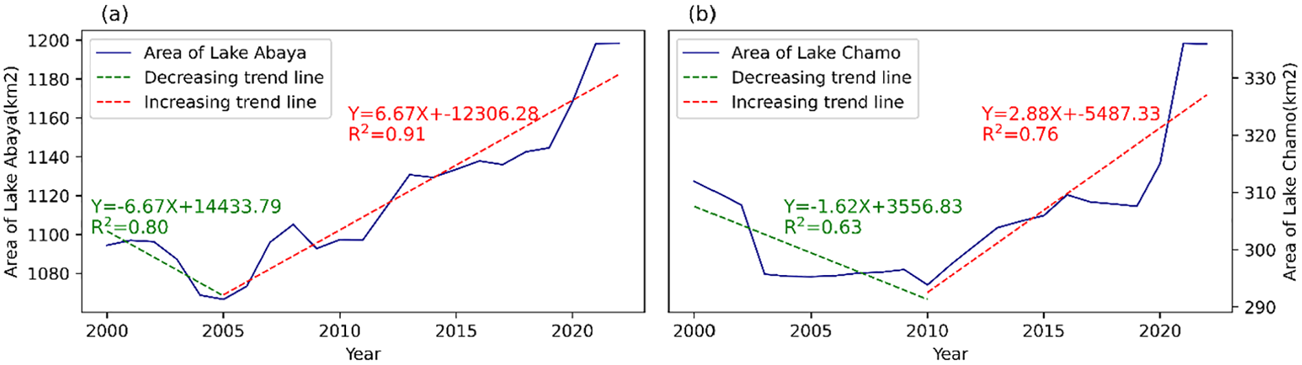
Long term annual area of Lake since 2000 to 2022: (a) annual area fluctuation plot of Lake Abaya and (b) annual area fluctuation plot of Lake Chamo.

Lake Abaya area dynamics

As shown in Figure 6(a), the area of Lake Abaya experienced a remarkable reduction between 2000 and 2005, declining from 1,094.56 km² to a minimum of 1,066.65 km². This decline could be attributed to various factors such as changes in precipitation, land-use patterns, or natural hydrological variability. The minimum observed area in 2005, 1,066.65 km², represents a critical point in the dynamics of Lake Abaya. However, an abrupt expansion occurred in the subsequent years, from 2005 to 2022, indicating a significant increment in annual area of the lake. The lake area experienced a substantial rise, reaching 1,198.35 km² by 2022 from 1,066.65 km² in 2005. This remarkable increase amounted to 131.70 km², signifying a substantial expansion of the lakes. Notably, this increment constituted a 12.35% expansion relative to the minimum observed lake area in 2005. The average rate of surface water area rise of Lake Abaya from 2005 to 2022 was 6.67 km² per year.

The significant expansion of Lake Abaya after 2005 could be linked to increased rainfall in the region and hydrological factors such as changes in groundwater flow and terrestrial water storage. Studies have been reported in other studies of Rift Valley lakes, where lake expansion is often linked to changes in hydrological inputs and catchment-level processes (Gebeyehu et al., 2019).

Lake Chamo area dynamics

Likewise, the area of Lake Chamo, as shown in Figure 6(b), experienced a noticeable reduction 311.92 km² in 2000 to 293.85 km² in 2010. However, the lake area increased substantially after 2010, reaching 336.04 km² by 2022. Notably, this expansion constitutes a 14.36% increase relative to the minimum observed lake area in 2010, with an average rate of rise 2.88 km² per year.

The fluctuations observed in Lake Chamo’s area align with the findings of other studies on lake dynamics in the region (Zekarias et al., 2021).

Factors influencing lake area changes

Understanding the factors influencing the changes in lake area is crucial for unraveling the complex causes of the expansion in Lake Chamo. To investigate the driving factors, several key environmental variables, including RF, TEMP, NDVI, SM, GWS, and TWS were analyzed. Figures 7 and 8 reveal the temporal trends of these variables for Lake Abaya and Lake Chamo, respectively.

Figure 7.

Selected variables and their time series trend over the study period of Abaya Lake.

Figure 8.

Selected variables and their time series trend over the study period (Chamo).

The investigation of factors influencing Lake Abaya’s water dynamics involved analyzing trends in RF, TEMP, NDVI, SM, GWS, and TWS. Figure 7 illustrates the trends of these variables over the study period. Analysis of time series data for Lake Abaya and its contributing catchment revealed an increasing trend in SM, GWS, and TWS (Figure 7(b), (d), and (f) respectively). These factors contribute to the expansion of the lake area by enhancing water availability. However, RF and NDVI demonstrated decreasing trends (Figure 7(a) and (e) respectively), suggesting that these factors may have inhibited the lake water availability. The increasing TEMP trend (Figure 7(c)), is counterintuitive to the lake’s expansion, as rising TEMP typically increase evapotranspiration, reducing water availability. However, despite this, the observed lake area expansion suggests that other factors may have played a dominant role in driving lake area changes, offsetting the impact of increased temperature.

In contrast, Lake Chamo showed increasing trends in RF, SM, GWS, and TWS (Figure 8(a), (b), (d), and (f) respectively), all of which positively affecting the lake’s area expansion. Similar to Lake Abaya, the NDVI for Lake Chamo showed a decreasing trend (Figure 8(c) and (e) respectively), indicating vegetation degradation in the catchment. The increase in water availability, as indicated by rising SM, GWS, and TWS, likely contributed to the lake’s expansion, despite the degrading vegetation conditions.

Both Lake Abaya and Lake Chamo exhibited similar characteristics regarding SM, GWS, TWS, and NDVI trends, indicating their potential influence on lake area increment. However, RF and TEMP exhibited contrasting trends between the two lakes. As RF decreased for Lake Abaya and increased for Lake Chamo, TEMP increase for Lake Abaya and decreased for Lake Chamo. These contrasting trends of the two lakes indicate the unique hydrological responses of each lake to environmental changes, reflecting the complex dynamics taking place in their respective ecosystems.

The vegetation degradation observed in both lakes’ catchments, indicated by the declining NDVI trend, is consistent with findings from land use and land cover change studies in the region. Studies by Ayalew et al. (2022); Gebeyehu et al. (2019); Woldeyohannes et al. (2020), and Zekarias et al. (2021) reported significant deforestation, agricultural expansion, and urbanization in the basin, leading to increased sediment inflow into the lakes. This sedimentation likely contributed to the expansion of lake areas by displacing water and raising lake levels.

Correlation analysis

The relationship between lake area and selected variables, RF, TEMP, NDVI, SM, GWS, and TWS of Lake Abaya and Lake Chamo region was examined to realize the response of lakes area to these variables (Abujayyab et al., 2021). The correlation matrices in Figures 9 and 10 provide insights into the strength and significance of the relationships between the selected variables and the lake area of both lakes. There were strong negative or positive significant relationships between the lake area and these variables (p < α = .05).

Figure 9.

Correlation matrix (correlation coefficients with corresponding p-values) of Lake Abaya.

Figure 10.

Correlation matrix (correlation coefficients with corresponding p-values) of Lake Chamo.

Lake Abaya

Figure 9 provides the correlation coefficients and corresponding p-values of the selected variables influencing the area of Lake Abaya. Among the variables, TEMP, NDVI, and TWS emerge as significant factors driving changes in the lake’s area. The strongest correlation, with a coefficient of .567, is observed between the lake area and TEMP, indicating a positive relationship with high statistical significance (p < .05). However, interpreting this correlation requires caution, as the positive association appears counterintuitive. Typically, an increase in temperature is expected to enhance evapotranspiration, leading to a reduction in water levels and, consequently, a decrease in the lake’s surface area (Adrian et al., 2009). The positive correlation between temperature and lake area may be attributed to the complex interplay between various hydrological factors, such as groundwater inflows, which could offset the expected evapotranspiration losses. Therefore, in this case, the rise in temperature is unlikely to be the primary driver of Lake Abaya’s surface area expansion. A negative correlation, if statistically significant, would more logically explain the influence of temperature on lake area reduction. The observed positive correlation may point to other indirect or complex interactions between temperature and hydrological processes.

The second-highest negative correlation coefficient of −.539 is found between the lake area of Abaya and NDVI of the contributing catchments. This inverse relationship (p < .05) indicates the essential role of vegetation cover in influencing the lake’s area dynamics. The decline in NDVI reflects the degradation of vegetation in the contributing catchments, which in turn leads to increased soil erosion and sediment inflow into the lake. Such sediment influx can fill the lake bed, displacing water and contributing to an apparent rise in the lake’s surface area. This process aligns with findings from other studies that emphasize the impact of land cover changes on sediment transport and its effect on lake morphology (Woldeyohannes et al., 2020).

TWS also exhibited a statistically significant positive correlation with the lake area, with a correlation coefficient of .531 (p < .05). This indicates the substantial role that changes in terrestrial water storage play in influencing the lake’s area. The rising trend of TWS in the Lake Abaya catchment during the study period suggests that the increase in terrestrial water contributed to the expansion of the lake’s surface. The positive correlation points to the interaction between terrestrial and lake water, where enhanced groundwater and soil moisture storage may have led to increased inflow, thus supporting the rise in lake area (Zekarias et al., 2021).

Overall, NDVI, and TWS have the most significant and direct influences on the surface area dynamics of Lake Abaya, while other variables RF, GWS, and SM exhibit weaker correlation implying more minor influence on the area dynamics.

Lake Chamo

Based on the correlation matrix shown in Figure 10, the correlation between lake area and the factors influencing was analyzed. A strong inverse correlation was observed between the Lake Abaya’s area and the NDVI of its contributing catchment, with a correlation coefficient of −.431, which is statistically significant (p < .05). This reveals the critical role of vegetation cover in shaping the lake’s area dynamics. The negative correlation indicates that as NDVI decreases, indicating vegetation degradation, and surface area of lake increases. This finding is consistent with studies that underscore the impact of vegetation decline on lake ecosystems through its effects on erosion and sedimentation (Fernández et al., 2007; Woldeyohannes et al., 2020).

The decreasing trend in NDVI suggests vegetation degradation in the catchment areas surrounding Lake Chamo, similar to the dynamics observed for Lake Abaya. This degradation accelerates soil erosion, resulting in an increased inflow of sediment into the lake. As sediment accumulates on the lake floor, it gradually displaces water, contributing to the apparent expansion of Lake Chamo’s surface area. This process emphasizes the interconnectedness between land cover changes, erosion, sediment transport, and lake morphology. Getaneh et al. (2024) pointed out the continuous vegetation degradation and land use changes, causing accelerate sedimentation rates, which can substantially alter the surface area and volume of lakes.

RF, TEMP, GWS, TWS, and SM exhibited statistically insignificant correlations with the lake’s surface area. Though these variables did not show a strong relationship in this analysis, it is important to recognize that they may still be relevant in specific contexts or when interacting with other factors not included in this study.

In comparison to Lake Abaya, where both NDVI and TWS were identified as major drivers of surface area dynamics, NDVI was the only statistically significant factor affecting Lake Chamo’s surface area. This difference may reflect the varying environmental and hydrological conditions between the two lakes, as well as the unique characteristics of their respective catchments.

Lake level validation

Before addressing the relationship between lake area and lake level, the accuracy of altimeter-derived lake level data was assessed. Validation accuracy for Lake Abaya was 0.88, and for Lake Chamo, it was 0.69, indicating a high correlation coefficient as depicted in Figure 11(a) and (b) respectively.

Figure 11.

Validation of lake level data: (a) altimeter lake level versus measured lake level and their coefficient of determination for Lake Abaya and (b) altimeter lake level versus measured lake level and their coefficient of determination for Lake Chamo.

Filling missing lake level values of Lake Chamo

To overcome the scarcity of lake level data for Lake Chamo, the lake level data of Lake Abaya was used to estimate the lake level data of Lake Chamo through a linear regression model. The plot showing the lake level data of Abaya against that of Chamo of the original altimeter lake level dataset, as shown in the Figure 12(a), yielded an R² value of .91, indicating a strong correlation between the two.

Figure 12.

The relationship of lake level of Abaya and Chamo: (a) before filling the missing lake level values of Chamo and (b) after filling the missing lake level values of Chamo.

The missing data periods in the Lake Chamo dataset were then filled using the regression function, resulting in an improved R² value of .98 after correction by substituting missing values with predicted values as presented in Figure 12(b). Given that Lake Abaya and Lake Chamo share a common basin and have similar hydro-meteorological settings, a linear regression model was deployed to relate lake level of the two lakes.

The relationship of lake area and lake level

The relationship between lake area and lake level is a fundamental aspect of understanding the dynamics of freshwater ecosystems. In Figure 13, the time series and correlation plots of lake area and lake level for Abaya and Chamo lakes is presented.

Figure 13.

(a) Time series of area and level of Lake Abaya, (b) correlation of area and level of Lake Abaya, (c) time series of area and level of Lake Chamo, and (d) correlation of area and level of Lake Chamo.

Figure 13(a) and (b) depict the time series and correlation plots of lake area and lake level for Lake Abaya, respectively. The graphs illustrate a strong correlation between the two variables, indicating that changes in lake area correspond closely with fluctuations in lake level. Specifically, the expansion in the area and the rise in level of Lake Abaya exhibit a high correlation coefficient of determination (R²) of .94. This strong correlation suggests that changes in lake level significantly influence the surface area of Lake Abaya, which could be attributed to factors such as precipitation, evaporation.

Similarly, Figure 13(c) and (d) show the time series and correlation plots of the area and level of Lake Chamo, respectively. Despite the scarcity of lake level data for Chamo, covering only the period from 2002 to 2016, the correlation between lake area and lake level remains strong. The correlation coefficient of determination (R²) for the relationship between lake level and lake area of Chamo is .80, indicating a substantial association between the two variables. This suggests that, despite data limitations, changes in lake level still have a notable impact on the surface area of Lake Chamo during the observed time period.

Overall, the findings underscore the importance of monitoring both lake area and lake level to gain insights into the dynamics of freshwater systems. The strong correlations observed in both Lake Abaya and Lake Chamo indicate the interdependence between these variables and emphasize the need for continued data collection and analysis to better understand and manage these valuable natural resources.

Modeling lake area and lake level relationship

Applying polynomial regression models to assess the relationship between lake area and lake level offers valuable intuitions into the dynamics of lake water. In this discussion, the implications of employing fourth-order and third-order polynomial regression models for Lake Abaya and Lake Chamo, respectively, are explored, based on the reported modeling and cross-validation results presented in Figure 14.

Figure 14.

(a) Fourth order polynomial model results plot for Lake Abaya, (b) Model cross validation for Lake Abaya, (c) fourth order polynomial model results plot for Lake Chamo, and (d) Model cross validation for Lake Chamo.

For Lake Abaya (see Figure 14(a) and (b)), the utilization of a fourth-order polynomial regression model produces compelling results. During the modeling phase, the fourth-order polynomial regression demonstrates a high level of explanatory power, with an R-squared (R²) value of .96. This indicates that approximately 96% of the variability in lake level can be accounted for by the model. Furthermore, the cross-validation result shows a negligible decrease in performance, with an R² value of .95. These findings suggest that the fourth-order polynomial regression model accurately captures the nonlinear relationship between lake area and level in Lake Abaya, both in terms of modeling and predictive capabilities.

Similarly, for Lake Chamo (see Figure 14(c) and (d)), the application of a third-order polynomial regression model provides valuable intuitions into the lake’s dynamics. Despite the slightly lower R² values compared to Lake Abaya, the third-order polynomial regression model demonstrates a strong explanatory power during the modeling phase, with an R² value of .86. This indicates that approximately 86% of the variability in lake level can be explained by the model. The cross-validation result maintains a reputable level of performance, with an R² value of .84. These findings suggest that the third-order polynomial regression model effectively captures the relationship between area and level in Lake Chamo, allowing for reliable predictions of lake level based on changes in area.

Conclusion

This study examined the dynamic nature of Abaya and Chamo lakes in Ethiopia’s Rift Valley using Landsat images and Altimeter-derived lake level data from 2000 to 2022 with Google Earth Engine. Significant expansions in the area, and rise in the level of the lakes were observed, highlighting the complex interaction of environmental and climatic factors.

The high accuracy achieved in lake water area extraction through the proposed MIRF classification method demonstrated the effectiveness of remote sensing techniques in monitoring lake dynamics. The overall accuracy ranged from 97.58% to 99.13%, while the Kappa Coefficient ranged from .95 to .98. Thus, this method offers a valuable tool for future studies aiming to understand and manage similar lake environments worldwide.

The results emphasized lake water surface area extraction using the MIRF classifier and the critical influence of factors such as soil moisture, groundwater storage, temperature, and vegetation status on the dynamics of these lakes. Notably, the strong correlation between lake area and NDVI stressed the ecological significance of maintaining catchment vegetation cover for both lakes. The study also elucidated the significant correlation between terrestrial water storage and lake area, indicating the interconnectedness of terrestrial and lake systems, especially in the case of Lake Abaya. Additionally, higher-order polynomial regression models representing lake area and lake level relationships were developed, yielding validation R² values of .95 and .84 for Lake Abaya and Lake Chamo, respectively.

Overall, this study contributes to the growing perception of lake dynamics and underlines the importance of continued monitoring and research efforts in freshwater resources management. By integrating remote sensing, statistical analysis, and hydrological modeling, enhances understanding of the complex interactions determining lake ecosystems and informs evidence-based conservation strategies for the long-term safeguarding of these precious natural resources.

Footnotes

Acknowledgements

The author expresses sincere gratitude to the Ethiopian Meteorology Institute (EMI) and the Ministry of Water and Energy of Ethiopia (MoWE) for providing the essential weather and lake level datasets.

Author contributions

Bewketu Assefa Mulu: Conceptualization, Data curation, methodology, software, Analysis, Investigation, visualization, writing original draft, Conceptualization, methodology, visualization, supervision, writing review and editing; Fasikaw Atanaw Zimale: Conceptualization, methodology, supervision, editing; Mulugeta Genanu Kebede: Conceptualization, methodology, supervision, editing. All authors have read and agreed to this version of the manuscript.

Funding

The author(s) received no financial support for the research, authorship, and/or publication of this article.

Declartion of Conflicting Interests

The author(s) declared no potential conflicts of interest with respect to the research, authorship, and/or publication of this article.

Data Availability Statement

All the data used for this research work are available from the author upon request.

ORCID iD

Bewketu Assefa Mulu

References

Abujayyab

S. K. M.

Almotairi

K. H.

Alswaitti

Amr

S. S. A.

Alkarkhi

A. F. M.

Taşoğlu

Hussein

A. M.

(2021). Effects of meteorological parameters on surface water loss in Burdur Lake, Turkey over 34 years Landsat Google Earth Engine time-series. Land, 10(12), Article 1301. https://doi.org/10.3390/land10121301

Adrian

Reilly

C. M. O.

Zagarese

Baines

S. B.

Hessen

D. O.

Keller

Livingstone

D. M.

Sommaruga

Straile

Van Donk

Weyhenmeyer

G. A.

Winder

(2009). Lakes as sentinels of climate change. Limnology and Oceanography, 54, 2283–2297.

Akgül

M. A.

Aksu

(2021). Areal precipitation estimation using satellite derived rainfall data over an irrigation area. Turkish Journal of Agriculture - Food Science and Technology, 9(2), 386–394. https://doi.org/10.24925/turjaf.v9i2.386-394.4061

Albarqouni

M. M. Y.

Yagmur

Bektas Balcik

Sekertekin

(2022). Assessment of spatio-temporal changes in water surface extents and lake surface temperatures using Google Earth Engine for lakes region, Türkiye. ISPRS International Journal of Geo-Information, 11(7), Article 407. https://doi.org/10.3390/ijgi11070407

Arora

Dixit

Pateriya

(2022). Assessment of water storage changes using Satellite Gravimetry and GLDAS observations over a part of Indus Basin, India. Water Conservation Science and Engineering, 7(4), 623–645. https://doi.org/10.1007/s41101-022-00169-6

Arora

Gujarati

Chandel

Pateriya

(2023). Assessment of river water dynamics and optically active water quality parameters over Punjab, based on cloud computing approach. In P. K. Rai (Ed.), Advances in water resources planning and sustainability (pp. 39–64). Springer.

Asfaw

Haile

A. T.

Rientjes

(2020). Combining multisource satellite data to estimate storage variation of a lake in the Rift Valley Basin, Ethiopia. International Journal of Applied Earth Observation and Geoinformation, 89, Article 102095. https://doi.org/10.1016/j.jag.2020.102095

Ayalew

A. D.

Wagner

P. D.

Sahlu

Fohrer

(2022). Land use change and climate dynamics in the Rift Valley Lake Basin, Ethiopia. Environmental Monitoring and Assessment, 194(10), Article 791. https://doi.org/10.1007/s10661-022-10393-1

Berhanu

K. G.

Lohani

T. K.

Hatiye

S. D.

(2024). Comparative evaluation of the dynamics of terrestrial water storage and drought incidences using multiple data sources: Tana sub-basin, Ethiopia. Journal of Water and Climate Change, 15(3), 1102–1119. https://doi.org/10.2166/wcc.2024.484

10.

Bewketu

(2015). Hydrodynamics of selected Ethiopian Rift Lakes [Unpublished MSc thesis]. Addis Ababa University.

11.

Chen

Zhang

Tian

(2017). Extraction of glacial lake outlines in Tibet Plateau using landsat 8 imagery and Google Earth Engine. IEEE Journal of Selected Topics in Applied Earth Observations and Remote Sensing, 10(9), 4002–4009. https://doi.org/10.1109/JSTARS.2017.2705718

12.

Chen

J. L.

Kang

Yang

Cao

(2020). Open-surface water bodies dynamics analysis in the Tarim River Basin (North-Western China), based on Google Earth Engine cloud platform. Water, 12(10), Article 2822.

13.

Chen

J. L.

Luo

W. B.

Wang

W. J.

Y. L.

Zou

Z. K.

Han

Huang

S. Z.

(2024). Influence of rainfall spatial variability on runoff simulation in Hilly irrigation areas. Applied Ecology and Environmental Research, 22(4), 3347–3359. https://doi.org/10.15666/aeer/2204_33473359

14.

Daniel

Ayenew

Fletcher

C. G.

(2019). Simulated surface and shallow groundwater resources in the Abaya-Chamo Lake basin, Ethiopia using a spatially-distributed water balance model. Journal of Hydrology: Regional Studies, 24, Article 100615. https://doi.org/10.1016/j.ejrh.2019.100615

15.

Dehghani

Torabi Poudeh

Izadi

(2022). Dissolved oxygen concentration predictions for running waters with using hybrid machine learning techniques. Modeling Earth Systems and Environment, 8(2), 2599–2613. https://doi.org/10.1007/s40808-021-01253-x

16.

Dehkordi

A. T.

Zoej

M. J. V.

Ghasemi

Ghaderpour

Hassan

Q. K.

(2022). A new clustering method to generate training samples for supervised monitoring of long-term water surface dynamics using Landsat data through Google Earth Engine. Sustainability, 14(13), Article 8046. https://doi.org/10.3390/su14138046

17.

Deng

Jiang

Tang

Ling

(2019). Long-term changes of open-surfacewater bodies in the Yangtze River Basin based on the google earth engine cloud platform. Remote Sensing, 11(19), Article 2213. https://doi.org/10.3390/rs11192213

18.

Dervisoglu

(2022). Investigation of long and short-term water surface area changes in coastal ramsar sites in Turkey with Google Earth Engine. ISPRS International Journal of Geo-Information, 11(1), Article 46. https://doi.org/10.3390/ijgi11010046

19.

Dong

Wang

Amankwah

S. O. Y.

Wei

Feng

(2021). Monitoring the summer flooding in the Poyang Lake area of China in 2020 based on Sentinel-1 data and multiple convolutional neural networks. International Journal of Applied Earth Observation and Geoinformation, 102, Article 102400. https://doi.org/10.1016/j.jag.2021.102400

20.

Fernández

Vega

J. A.

Fonturbel

Pérez-Gorostiaga

Jiménez

Madrigal

(2007). Effects of Wildfire, Salvage Logging and Slash. Land Degradation & Development, 607, 591–607. https://doi.org/10.1002/ldr

21.

Feyisa

G. L.

Meilby

Fensholt

Proud

S. R.

(2014). Automated Water Extraction Index: A new technique for surface water mapping using Landsat imagery. Remote Sensing of Environment, 140, 23–35. https://doi.org/10.1016/j.rse.2013.08.029

22.

Funk

Peterson

Landsfeld

Pedreros

Verdin

Shukla

Husak

Rowland

Harrison

Hoell

Michaelsen

(2015). The climate hazards infrared precipitation with stations—A new environmental record for monitoring extremes. Scientific Data, 2(1), 1–21. https://doi.org/10.1038/sdata.2015.66

23.

Gebeyehu

A. E.

Chunju

Yihong

(2019). Assessment and mapping of land use change by remote sensing and GIS: A case study of Abaya Chamo Sub-basin, Ethiopia. Nature Environment and Pollution Technology, 18(2), 549–554.

24.

Gebrehiwot

K. A.

Fanta

Gebrewahid

M. G.

Hishe

B. K.

(2022). Analysis of surface area fluctuation of the Haramaya Lake using remotely sensed satellite imagery. OMO International Journal of Sciences, 5(2), 24–35. https://doi.org/10.59122/13469ac

25.

Getaneh

Z. A.

Demissew

Woldu

(2024). Spatiotemporal dynamics of land use land cover change and its drivers in the western part of Lake Abaya, Ethiopia. PeerJ, 12(9), 1–20. https://doi.org/10.7717/peerj.17892

26.

Ghorbanian

Zaghian

Asiyabi

R. M.

Amani

Mohammadzadeh

Jamali

(2021). Mangrove ecosystem mapping using sentinel-1 and sentinel-2 satellite images and random forest algorithm in google earth engine. Remote Sensing, 13(13), Article 2565. https://doi.org/10.3390/rs13132565

27.

Gómez Fernández

Salas López

Rojas Briceño

N. B.

Silva López

J. O.

Oliva

. (2022). Dynamics of the Burlan and pomacochas lakes using SAR data in GEE, machine learning classifiers, and regression methods. ISPRS International Journal of Geo-Information, 11(11), Article 534. https://doi.org/10.3390/ijgi11110534

28.

Hackländer

Jung

(2021). Land potential assessment and trend-analysis using 2000–2021 FAPAR monthly time-series at 250 m spatial resolution. PeerJ, 12, Article e16972.

29.

Havens

Paerl

Phlips

Zhu

Beaver

Srifa

(2016). Extreme weather events and climate variability provide a lens to how shallow lakes may respond to climate change. Water, 8(6), Article 229. https://doi.org/10.3390/w8060229

30.

Huang

Chen

Fang

Liu

(2023). Monitoring surface water area changes in the aral sea basin using the Google Earth engine cloud platform. Water, 15(9), Article 1729.

31.

Jiang

Ling

Wang

Peng

Wang

(2021). Surface water extraction and dynamic analysis of baiyangdian lake based on the google earth engine platform using sentinel-1 for reporting sdg 6.6.1 indicators. Water, 13(2), Article 138. https://doi.org/10.3390/w13020138

32.

Kandasamy

Baret

Verger

Neveux

Weiss

(2013). A comparison of methods for smoothing and gap filling time series of remote sensing observations – Application to MODIS LAI products. Biogeosciences, 10(6), 4055–4071. https://doi.org/10.5194/bg-10-4055-2013

33.

Kandekar

V. U.

Pande

C. B.

Rajesh

Kadam

S. D. G. S. A

. (2021). Surface water dynamics analysis based on sentinel imagery and Google Earth Engine Platform: A case study of Jayakwadi dam. Sustainable Water Resources Management, 7(3), Article 44. https://doi.org/10.1007/s40899-021-00527-7

34.

Kebede

M. G.

Wang

(2020). Remote sensing-based river discharge estimation for a small river flowing over the high mountain regions of the Tibetan Plateau. International Journal of Remote Sensing, 41(9), 3322–3345. https://doi.org/10.1080/01431161.2019.1701213

35.

Khorrami

Ali

Sahin

O. G.

Gunduz

(2023). Model-coupled GRACE-based analysis of hydrological dynamics of drying Lake Urmia and its basin. Hydrological Processes, 37(5), Article e14893. https://doi.org/10.1002/hyp.14893

36.

Wang

Cheng

Wang

Zhou

Altansukh

(2022). Deep learning empowers the Google Earth Engine for automated water extraction in the Lake Baikal Basin. International Journal of Applied Earth Observation and Geoinformation, 112, Article 102928. https://doi.org/10.1016/j.jag.2022.102928

37.

Long

Huang

Han

Zhao

Wada

(2019). High-temporal-resolution water level and storage change data sets for lakes on the Tibetan Plateau during 2000–2017 using multiple altimetric missions and Landsat-derived lake shoreline positions. Earth System Science Data, 11(4), 1603–1627.

38.

Zhang

Tao

Yao

(2021). Integrated model projections of climate change impacts on water-level dynamics in the large Poyang Lake (China). Hydrology Research, 52(1), 43–60. https://doi.org/10.2166/NH.2019.064

39.

Bolin

Peiqing

Tingyuan

W. G.

(2020). Delineation water of pearl river basin using Landsat images from Google Earth Engine. The International Archives of the Photogrammetry, Remote Sensing and Spatial Information Sciences, 42, 5–10.

40.

Luo

Liu

Guo

Shao

(2021). Using time series sentinel-1 images for object-oriented crop classification in google earth engine. Remote Sensing, 13(4), Article 561. https://doi.org/10.3390/rs13040561

41.

Matarira

Mutanga

Naidu

(2022). Google earth engine for informal settlement mapping: A random forest classification using spectral and textural information. Remote Sensing, 14(20), Article 5130. https://doi.org/10.3390/rs14205130

42.

Nguyen

Ombadi

Sorooshian

Hsu

Aghakouchak

Braithwaite

(2018). The PERSIANN family of global satellite precipitation data: A review and evaluation of products. Hydrology and Earth System Sciences, 22(11), 5801–5816.

43.

Noi Phan

Kuch

Lehnert

L. W

. (2020). Land cover classification using google earth engine and random forest classifier-the role of image composition. Remote Sensing, 12(15), Article 2411. https://doi.org/10.3390/RS12152411

44.

Olawoyin

Acheampong

P. K.

(2017). Objective assessment of the Thiessen polygon method for estimating areal rainfall depths in the River Volta catchment in Ghana. Ghana Journal of Geography, 9(2), 151–174.

45.

Oliphant

A. J.

Thenkabail

P. S.

Teluguntla

Xiong

Gumma

M. K.

Congalton

R. G.

Yadav

(2019). Mapping cropland extent of Southeast and Northeast Asia using multi-year time-series Landsat 30-m data using a random forest classifier on the Google Earth Engine Cloud. International Journal of Applied Earth Observation and Geoinformation, 81, 110–124. https://doi.org/10.1016/j.jag.2018.11.014

46.

Oyebode

(2019). Evolutionary modelling of municipal water demand with multiple feature selection techniques. Journal of Water Supply: Research and Technology - AQUA, 68(4), 264–281. https://doi.org/10.2166/aqua.2019.145

47.

Chen

Liu

Zhi

Zhang

(2022). Mapping large area tea plantations using progressive random forest and Google Earth Engine. Journal of Applied Remote Sensing, 16(2), 1–22. https://doi.org/10.1117/1.jrs.16.024509

48.

Ren

Fang

Zhang

Shi

(2020). Comparison of eight filter-based feature selection methods for monthly streamflow forecasting – Three case studies on CAMELS data sets. Journal of Hydrology, 586, Article 124897. https://doi.org/10.1016/j.jhydrol.2020.124897

49.

Richey

A. S.

Thomas

B. F.

M. H.

Reager

J. T.

Famiglietti

J. S.

Voss

Swenson

Rodell

(2015). Quantifying renewable groundwater stress with GRACE. Water Resources Research, 51(7), 5217–5237. https://doi.org/10.1002/2015WR017349

50.

Running

S. W.

Zhao

(2019). User’s guide daily GPP and annual NPP (MOD17A2H/A3H) and year-end gap- filled (MOD17A2HGF/A3HGF) products NASA earth observing system MODIS land algorithm (for collection 6). NASA EOSDIS Land Processes DAAC. https://lpdaac.usgs.gov/documents/379/MOD17_User_Guide_V6.pdf

51.

Schwatke

Dettmering

Bosch

Seitz

(2015). DAHITI – an innovative approach for estimating water level time series over inland waters using multi-mission satellite altimetry. Hydrology and Earth System Sciences, 19(10), 4345–4364. https://doi.org/10.5194/hess-19-4345-2015

52.

Senanayake

I. P.

Yeo

(2023). A random forest-based multi-index classification (RaFMIC) approach to mapping three-decadal inundation dynamics in dryland wetlands using Google Earth Engine. Remote Sensing, 15(5), Article 1263.

53.

Sodhi

T. S.

Dahiphale

Arora

(2024). Assessment of Water Dynamics and Water Quality Parameters over Gobind Sagar Reservoir, India, Based on High-Resolution Remote Sensing Approach. Water Conservation Science and Engineering, 9(2). https://doi.org/10.1007/s41101-024-00268-6

54.

Tang

Baig

M. H. A.

Fang

Wang

(2022). Large-scale surface water mapping based on Landsat and sentinel-1 images. Water, 14(9), Article 1454. https://doi.org/10.3390/w14091454

55.

Temesgen

Akil

Wendemeneh

(2022). The impact of climate change on the availability of irrigation water at the rift valley lakes basin in Southern Ethiopia: A review. Journal of Digital Food, Energy & Water Systems, 3(1), 1–15. https://doi.org/10.36615/digitalfoodenergywatersystems.v3i1.1281

56.

Tercan

Atasever

U. H.

(2021). Effectiveness of autoencoder for lake area extraction from high-resolution RGB imagery: An experimental study. Environmental Science and Pollution Research, 28(24), 31084–31096. https://doi.org/10.1007/s11356-021-12893-y

57.

Tew

Y. L.

Tan

M. L.

Samat

Chan

N. W.

Mahamud

M. A.

Sabjan

M. A.

. . . Wee

S. T.

(2022). Comparison of three water indices for tropical aquaculture ponds extraction using Google Earth Engine. Sains Malaysiana, 51(2), 369–378. https://doi.org/10.17576/jsm-2022-5102-04

58.

VanDeWeghe

Lin

Jayaram

Gronewold

A. D.

(2022). Changes in Large Lake Water Level Dynamics in Response to Climate Change. Frontiers in Water, 4(April), 1–12. https://doi.org/10.3389/frwa.2022.805143

59.

Vasilevskiy

Wang

Pozdniakov

Wang

Zhang

(2022). Simulating River/Lake – Groundwater exchanges in arid river basins: An improvement constrained by lake surface area dynamics and evapotranspiration. Remote Sensing, 14(7), Article 1657.

60.

Wang

Jia

Chen

Wang

(2018). Long-term surface water dynamics analysis based on Landsat imagery and the Google Earth Engine Platform: A case study in the middle Yangtze River Basin. Remote Sensing, 10(10), Article 1635. https://doi.org/10.3390/rs10101635

61.

Wang

Zhou

Wang

Zhao

(2023). Flood monitoring in the middle and lower basin of the Yangtze river using Google Earth Engine and machine learning methods. ISPRS International Journal of Geo-Information, 12(3), Article 129.

62.

Wang

Xia

Qin

Niu

Pan

(2020). Dynamic monitoring of surface water area during 1989–2019 in the hetao plain using Landsat data in Google Earth Engine. Water, 12(11), Article 3010.

63.

Wei

Bao

Hou

Miao

(2020). A water body extraction methods comparison based on Fengyun Satellite data: A case study of Poyang Lake Region, China. Remote Sensing, 12(23), Article 3875. https://doi.org/10.3390/rs12233875

64.

Woldeyohannes

Cotter

Biru

W. D.

Kelboro

(2020). Assessing changes in ecosystem service values over 1985–2050 in response to land use and land cover dynamics in Abaya-Chamo basin, Southern Ethiopia. Land, 9(2), Article 37. https://doi.org/10.3390/land9020037

65.

Wulder

M. A.

Masek

J. G.

Cohen

W. B.

Loveland

T. R.

Woodcock

C. E.

(2012). Opening the archive: How free data has enabled the science and monitoring promise of Landsat. Remote Sensing of Environment, 122, 2–10. https://doi.org/10.1016/j.rse.2012.01.010

66.

Xia

Zhao

Qin

Yang

Cui

Song

Jin

Meng

(2019). Changes in water surface area during 1989–2017 in the Huai River Basin using Landsat data and Google earth engine. Remote Sensing, 11(15), Article 1824. https://doi.org/10.3390/rs11151824

67.

(2006). Modification of normalised difference water index (NDWI) to enhance open water features in remotely sensed imagery. International Journal of Remote Sensing, 27(14), 3025–3033. https://doi.org/10.1080/01431160600589179

68.

Xiao

Deng

Chen

(2021). Extraction of built-up area using multi-sensor data—A case study based on Google earth engine in Zhejiang Province, China. International Journal of Remote Sensing, 42(2), 389–404. https://doi.org/10.1080/01431161.2020.1809027

69.

R. G.

Qiao

Y. J.

Cao

Y. J.

(2019). Extraction of rivers and lakes on tibetan plateau based on google earth engine. International Archives of the Photogrammetry, Remote Sensing and Spatial Information Sciences, 42, 1797–1801. https://doi.org/10.5194/isprs-archives-XLII-2-W13-1797-2019

70.

Yang

Chen

Wang

Yang

Chen

(2020). Combined use of Sentinel-2 and Landsat 8 to monitor water surface area dynamics using Google Earth Engine Combined use of Sentinel-2 and Landsat 8 to monitor water surface area dynamics using Google Earth Engine. Remote Sensing Letters, 11(7), 687–696. https://doi.org/10.1080/2150704X.2020.1757780

71.

Yilmaz

O. S.

(2023). Spatiotemporal statistical analysis of water area changes with climatic variables using Google Earth Engine for Lakes Region in Türkiye. Environmental Monitoring and Assessment, 195(6), Article 735. https://doi.org/10.1007/s10661-023-11327-1

72.

Yue

Zhu

Yuan

Shen

(2023). A fully automatic and high-accuracy surface water mapping framework on Google Earth Engine using Landsat time-series. International Journal of Digital Earth, 16(1), 210–233. https://doi.org/10.1080/17538947.2023.2166606

73.

Zekarias

Govindu

Kebede

Gelaw

(2021). Heliyon geospatial analysis of wetland dynamics on lake Abaya-Chamo, the main Rift Valley of Ethiopia. Heliyon, 7, Article e07943. https://doi.org/10.1016/j.heliyon.2021.e07943

74.

Zhang

Wei

Wang

Long

(2021). Assessment of annual composite images obtained by Google Earth Engine for urban areas mapping using random forest. Remote Sensing, 13(4), Article 48. https://doi.org/10.3390/rs13040748

75.

Zhao

(2019). Long-term dynamic of Poyang Lake surface water: A mapping work based on the Google Earth Engine cloud platform. Remote Sensing, 11(3), Article 313. https://doi.org/10.3390/rs11030313

76.

Zhao

Feng

Xie

Zhu

Zhang

(2023). Extraction of long time series wetland information based on Google Earth Engine and random forest algorithm for a plateau lake basin – A case study of Dianchi Lake, Yunnan Province, China. Ecological Indicators, 146, Article 109813. https://doi.org/10.1016/j.ecolind.2022.109813

77.

Zhou

Dong

Xiao

Liu

Zou

(2019). Science of the total environment continuous monitoring of lake dynamics on the Mongolian Plateau using all available Landsat imagery and Google Earth Engine. Science of the Total Environment, 689, 366–380. https://doi.org/10.1016/j.scitotenv.2019.06.341

Remote Sensing-Based Long-Term Assessment of Water Dynamics and Influencing Factors in Abaya and Chamo Lakes,East African Rift Valley,Ethiopia

Abstract

Keywords

Introduction

Study Area

Data and Data Sources

Landsat 5, Landsat 7ETM+, and Landsat 8

Altimeter-derived lake level data

Rainfall and temperature data

Normalized Difference Vegetation Index (NDVI)

Groundwater storage, terrestrial water storage, and soil moisture

Methodology

Landsat image pre-processing

Rainfall and temperature data preparation

Random Forest classifier

Lake water extraction using multiple-index based RF

Accuracy assessment metrics

Statistical analysis

Validation of altimeter-derived lake level data

Validation of rainfall data

Modeling lake area and lake level relationship

Results and Discussion

Accuracy assessment of the extracted lake water map

Area dynamics of Lake Abaya and Lake Chamo

Lake Abaya area dynamics

Lake Chamo area dynamics

Factors influencing lake area changes

Correlation analysis

Lake Abaya

Lake Chamo

Lake level validation

Filling missing lake level values of Lake Chamo

The relationship of lake area and lake level

Modeling lake area and lake level relationship

Conclusion

Footnotes

Acknowledgements

Author contributions

Funding

Declartion of Conflicting Interests

Data Availability Statement

ORCID iD

References