Sage Journals: Discover world-class research

Abstract

Crop modeling is a powerful tool for estimating yield and water use efficiency, and it plays an important role in determining water management strategies. Under the condition of scarce water supply and drought, deficit irrigation can lead to greater economic gains by maximizing yield per unit of water. Studies have shown that deficit irrigation significantly increased yield, crop evapotranspiration, and water use efficiency as compared to full irrigation requirement. However, this approach requires precise knowledge of crop response to water as drought tolerance varies considerably by growth stage, species and cultivars. This study was conducted in Lasta district, for two successive years to evaluate the effects of water shortage on potato production and water use efficiency, as well as to test the AquaCrop model for potato-producing areas. The irrigation water levels for potatoes were 100%, 75%, and 50% of crop evapotranspiration (ETc). Six treatments were arranged using a randomized complete block design. Climate, soil, and crop data were calibrated using observed weather parameters, and measured crop parameters conducted in the 2018/19 growing season. The model was validated using the observed data conducted in the 2019/20 growing season. The calibration of the model revealed a good fit for canopy cover (CC) with a coefficient of determination (R²) = .98, Root mean square error (RMSE) = 9.6%, Nash-Sutcliffe efficiency (E) = 0.92, index of agreement (d) = 0.98, and coefficient of residual moss (CRM) = −0.07, and good prediction for biomass (R² = .98, RMSE = 1.8 t ha⁻¹, E = 0.96, d = 0.99, CRM = −0.13). Similarly, the validation result showed good fit for CC by 100% water application at development and mid growth season and a 75% water applied at the other stages (R² = .98, RMSE = 9.4%, E = 0.94, d = 0.98, CRM = −0.12). The AquaCrop model is simple to use, requires fewer input data, and has a high level of simulation precision, making it a useful tool for forecasting crop yield under deficit irrigation and water management to increase agricultural water efficiency in data-scarce areas.

Keywords

Biomass calibration canopy cover validation water use efficiency

Introduction

Potatoes (Solanum sp.) are the fifth most common crop globally, after sugar cane, maize, rice, and wheat (Montoya et al., 2016). It is one of the tuber crops grown in Ethiopia by more than one million farmers (CSA, 2018/2019), and it is also blessed with ideal climatic, soil, and topographic characteristics for potato cultivation. Potato is regarded as a high-potential food security crop because of its ability to provide a high yield of high-quality output per unit input with a crop cycle that is typically fewer than 120 days (Hirpa et al., 2010). The national average yield is about 14.2 tons ha⁻¹, which is at this time low as opposed to the world’s average output of 20.95 t ha⁻¹ (CSA, 2018/2019). Drought and flood, pests and diseases, soil erosion, the shift in rainfall pattern, and water quality issues are the leading causes for decreasing suitable water availability for growing potatoes (Deressa et al., 2009).

As a result, in order to produce more crops per drop while saving irrigation resources, higher water utilization efficiency for potato production is required. The limited availability of water resources needs the development of new approaches to save water and energy, the utmost of which should emphasize in improving water use efficiency (Shahnazari et al., 2007; Soomro et al., 2020). To ensure food security, it is essential to use the water wisely in order to increase food production while saving water as much as possible or to increase field crops’ water use productivity. The world’s population is growing by the day, posing a serious threat to future agricultural production, particularly in areas where water is the scarcest resource. Deficit irrigation is an improvement technique in which irrigation is applied during drought-sensitive growth stages of a crop (Geerts & Raes, 2009). It is a practice, which enhances the economic use of water (Domínguez et al., 2012; Fereres & Soriano, 2007); moreover, this approach can have a resilient effect on potato crops, by means of declines in crop yield and tuber quality (Fabeiro et al., 2001; Gebremedhin et al., 2015; Ierna & Mauromicale, 2012; Kashyap & Panda, 2003; Onder et al., 2005; Shock et al., 1998; Vos & Haverkort, 2007).

AquaCrop is a water-driven model that may be used to aid decision-making in planning and scenario analysis in a variety of seasons and locales (Corbari et al., 2021; Foster et al., 2017; Mibulo & Kiggundu, 2018). Despite its simplicity, the model elaborates on the fundamental processes involved in crop productivity and the response to water deficiencies, both physiologically and agronomically (Tefera & Mitiku, 2021). AquaCrop can also be used to research and evaluate another management strategy for increasing water productivity and achieving more sustainable water use (Amirouche et al., 2021; Bessembinder et al., 2005). The model simulates the variation in crop yield and biomass for the different irrigation water scenarios. Observing the daily water balance is required to consider the incoming and outgoing water. Development of the most favorable strategies in using and managing available water resources in the agricultural sector is a critical issue (Smith, 2000). Crop development models have been developing along with the growth of computer technology since the 1960s, which can offer the simulation of plant physiological processes and crop growth and development (Boote et al., 1998).

The AquaCrop model focuses on water input as the main factor limiting crop growth, especially in arid and semiarid regions (Bradford & Hsiao, 1982). According to Geerts and Raes (2009) and Heng et al. (2009), in order to evaluate the effect of changes in irrigation water quantity using the AquaCrop model for quinoa, sunflower, and maize in, the critical parameters for calibration, including such normalized water productivity, canopy cover, and total biomass, should be tested under a variety of environment, soil, cultivar, irrigation technique, and field management conditions.

Drought is the main climate-linked risk in the northeastern Amhara especially North Wollo and Wag-Himra and generally in some parts of northern Ethiopia. So, deficit irrigation could be a promising irrigation water management technique for these areas, allowing farmers to apply restricted amounts of water to their crops in the time and amount necessary for optimum crop water productivity. The objective of this study is to evaluate the effects of water shortage on potato production and water use efficiency and assess the performance of the AquaCrop model for potato production under deficit irrigation in Lasta district, North Wollo, Ethiopia.

Material and Methods

Study area description

The research was conducted for 2 years in 2018/19 and 2019/20 at Kechne Abeba irrigation schemes at Lasta woreda, North Wollo (Figure 1). The geographical location of the area is between 11°57′38.44″ latitude and 39°4′4.91″ longitude with 2,103 m of above sea level. The mean long-term annual rainfall (January 2000–March 2020) in the area is about 799.3 mm and it is erratic and uneven in distribution. The long-term average minimum and maximum temperatures in the area is 11.8°C and 27.4°C, respectively (Figure 2). The study site was chosen to be a representative of the woreda’s diverse soil and climate conditions. The area is intensively cultivated and the production is subsistence farming with a main practice of rain-fed agriculture.

Figure 1.

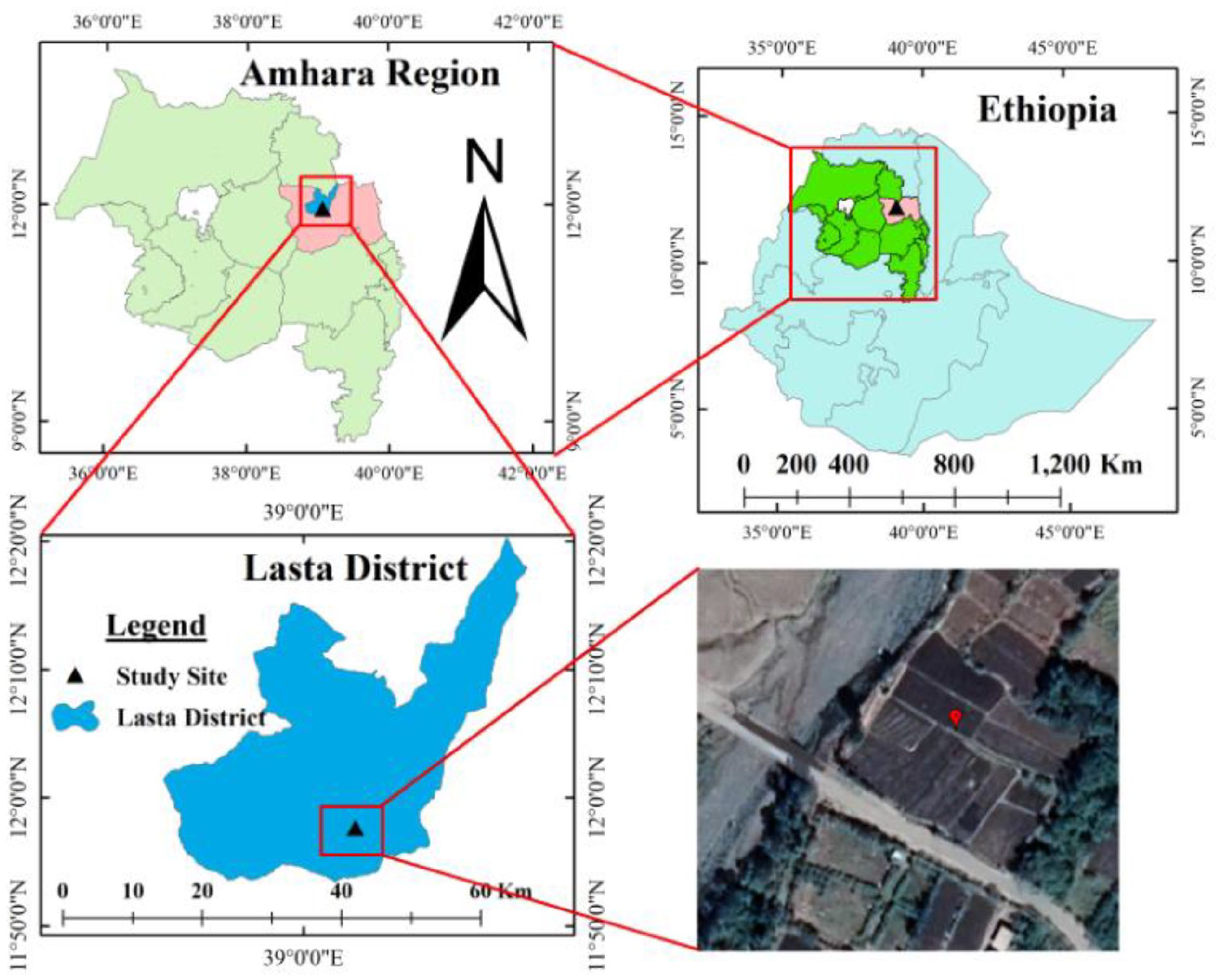
Location map of the study area in Amhara Region, Ethiopia.

Figure 2.

The weather conditions for 2018/19 (a) and 2019/20 crop growing season (b).

Treatment and experimental design

The design of the experiment was based on a randomized complete block design with three replications. In the field experiment, three irrigation treatments (100%, 75%, and 50%) with four growth stages of potato water application methods were tested (Table 1). The plot size of the experiment was 3.00 m × 3.75 m and the spacing among plots (P) and each block was 1 m and the total experimental area was 23.00 m × 13.25 m. The test crop potato (Belete variety) was selected since it is widely used in the area and also recommended for the area. The tubers were directly sown on October 16, 2018, and November 20, 2019. Well, sprouted potato tubers were planted on prepared ridges with the spacing of 75 by 30 cm between row and plants, respectively (Abdalhi & Jia, 2018; Beshir et al., 2018; Gebremedhin et al., 2015). In the 2018/19 and 2019/20 growing seasons, harvesting occurred when tubers reached maturity, which was 105 days after planting (DAP).

Table 1.

Total number of treatment combinations.

Treatment	Initial stage (%)	Potato crop growth stages		Late season stage (%)
Treatment	Initial stage (%)	Development stage (%)	Mid-season stage (%)	Late season stage (%)
T1	100	100	100	100
T2	75	75	75	75
T3	75	100	100	75
T4	50	100	100	50
T5	75	100	100	50
T6	100	75	75	50

Fertilizer was added at the rate of 300 kg ha⁻¹ urea half at planting (AP) and a half at 45 DAP and 50 kg ha⁻¹ triple superphosphate AP. The irrigation water was applied at 5 days intervals. All plots were irrigated with an equivalent volume of water prior to planting, up to the field capacity limits. For each treatment, weeding, furrow maintenance, fertilizer application, water application, diseases, and pest management techniques were applied on time and in the same order.

The whole field layout of the experiment is clearly indicated in Figure 3 and Table 1.

Figure 3.

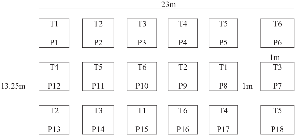
Layout of field experimental design.

Water requirement of potato

The fixed schedule and crop water demand for irrigation were determined using the CROPWAT computer model version 8.0, according to FAO 56 methodology (Allen et al., 1998). The crop coefficients (Kc) used in the reference irrigation treatment 100% (de la Casa et al., 2013; Razzaghi et al., 2017) which would have been the difference as per the vegetative growth stage of the potato crops 0.50 at the onset of growth, 1.15 at tuber formation, and 0.75 before ripening. The Kc for each growth stage was obtained from Allen et al. (1998) and crop evapotranspiration (ETc, mm) was determined using equation (1).

E T_{C} = E T_{O} * K_{C}

(1)

Where ETo is reference evapotranspiration in mm. Since it would be based on evapotranspiration, it is able to quantify net irrigation water demand (NIR) by subtracting effective rainfall (Pe) during the experimental season, which can be described using equation (2).

N I R = E T_{C} - P e

(2)

Furrow irrigation application efficiencies, in general, vary from 45% to 60% (Allen et al., 1998). Using equation (3), the requirement of gross irrigation (GIR) was calculated with an application efficiency (Ea) of 60%.

G I R = \frac{N I R}{E a}

(3)

AquaCrop model input data

It’s a crop water productivity model that simulates herbaceous crop yield response to water (Steduto et al., 2012). The setup of the model needs input data containing climatic parameters, crop, soil and field, and irrigation management data (Figure 4). On the other hand, the model consists of a complete set of input parameters that were selected and adjusted for different soil or crop types.

Figure 4.

Required input data for AquaCrop.

Climate data

The weather parameter was collected from Lalibela meteorological station located closer to the experimental farm. The model requires daily values meteorological data and annual mean atmospheric carbon dioxide concentrations. The ETo values were also calculated using daily meteorological data by the ETo calculator. The model uses 369.41 ppm as a reference standard for atmospheric carbon dioxide concentrations (Steduto et al., 2012).

Crop parameters

Canopy cover, above-ground biomass, tuber yield, and plant height data samples were taken out every 20 days for each irrigation treatment and replicated based on the recommendation stated in Bitri et al. (2014) and Karunaratne et al. (2011). The overhead mobile camera was used to capture the canopy cover. Then the captured picture was analyzed using GreenCrop Tracker image analyzer software (Kale, 2016). At each sample, two plants were removed from each experimental plot, and the dry biomass of leaves, stems, and tubers was collected (Montoya et al., 2016).

The above-ground dry biomass of each sample was determined by weighing it after it had been held in an oven for 48 hours at 65°C (Abedinpour et al., 2012) and the tuber dry matter for 72 hours at 65°C (Gebremedhin et al., 2015). The date of emergence, initial and maximum canopy cover, period of flowering, the start of senescence, and maturity were recorded. In addition, the coefficient of the crop for transpiration at full canopy cover, canopy decline coefficient, soil water depletion beginnings for prevention of leaf growth and transpiration, and canopy senescence acceleration are used as suggested by Hsiao et al. (2009). Since the criterion could be applied to a wide range of conditions and should not be limited to a single crop cultivar (Heng et al., 2009).

Soil characteristics

The physical and chemical properties such as soil texture, EC, pH, organic matter, bulk density, field capacity, permanent wilting point, and saturation of soil were analyzed and characterized in samples taken from the study area at different depths of 0 to 20, 20 to 40, 40 to 60 cm and three samples across the experimental field. The saturated hydraulic conductivity was determined using the empirical equations’ pedo transfer function (Saxton & Rawls, 2006). The gravimetric method was used to assess the soil moisture content and measured as a dry weighted fraction (Demelash & Alamirew, 2011). In the laboratory, the water content at FC and PWP were determined by applying 0.33 and 15 bars to a saturated soil sample, respectively, using a pressure plate.

Irrigation and field management

Irrigation management consists of data applying to both the conditions of full irrigation and deficit irrigation with four growth stages. In the deficit, irrigation water was applied the same day as the entirely irrigated plot, but the irrigation depths were decreased to 75% and 50% of the full irrigation. Water was applied in a known volume of watering cane to control the quantity of water entering each furrow of the experimental plot (Yihun, 2015). The volume of applied water (V, litters) can be calculated as follows equation (4).

V = A * D

(4)

Where A = irrigated plot (m²), D = depth of application (mm)

The field management components were recorded like the soil fertility levels, weed infestation, irrigation method, application depth and time of irrigation event, and furrow end bunds to remove surface runoff. Equation (5) was used to calculate water use efficiency (WUE), which indicates the amount of yield (Y, kg ha⁻¹) given per unit of water used (ETc, m³ ha⁻¹) and evaluates the most efficient use of water.

W U E = \frac{Y}{E T_{C}}

(5)

Model calibration

The model was performed via an iterative method that provided the data values which better simulated the primary crop growth variables canopy cover, biomass, crop yield, and water use efficiencies. These parameters are calibrated for the optimal goodness of match between both the measured and the simulated values (Afsharmanesh et al., 2014; Afshar & Neshat, 2013; Gebreselassie et al., 2015). The crop cultivar-dependent conservative and non-conservative parameters were regarded as constants. The non-conservative parameters were adjusted according to the field measurements. The crop growth coefficient (CGC) and crop senescence coefficient (CDC), as well as normalized water productivity (WP*), are conservative parameters that are calibrated using field sample results. The CGC and CDC were calculated using the estimates suggested by Raes et al. (2012b) and data such as maximum canopy cover (CCx) and initial canopy cover (CC₀). Thus, the CGC and CDC are determined using a nonlinear resolve to achieve the best possible match between the measured and simulated canopy cover.

Model validation

The model was run with the experimental data for the year 2019/20 growing season and then the predicted values were compared to the experiment’s actual results, and the model validation output statistics were assessed.

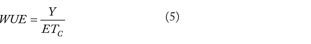
Model evaluation

During the calibration and validation processes, the AquaCrop model simulation findings of water use efficiency, biomass, yield, and canopy cover were evaluated. The prediction error statistics were used to verify the internal consistency between the simulated and observable values. To evaluate the model’s efficiency (performance), the following statistical approaches were used. The total values or average deviation of measured values from determined values is indicated by the normalized root mean square error (NRMSE or CV). Equation (6) was used to calculate the NRMSE formula.

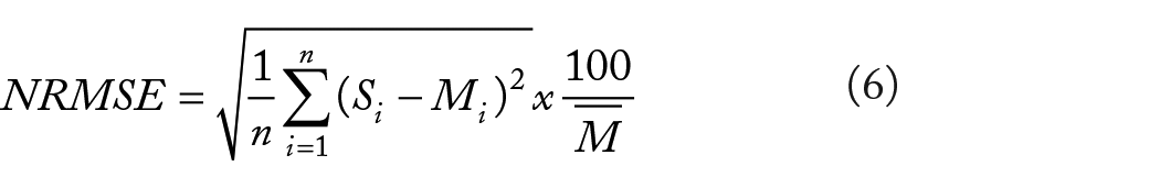
N R M S E = \sqrt{\frac{1}{n} \sum_{i = 1}^{n} {(S_{i} - M_{i})}^{2}} x \frac{100}{\bar{M}}

(6)

Where S_i and M_i are the simulated and measured values, separately, $\bar{M}$ is mean of measured value and n is a number of observations. The NRMSE unit is the same for all variables, and the average of the n measured results was used.

The root mean square error (RMSE) represents a measurement of the total, or it is the mean values of M_i mean deviation between the observed and simulated values which is a synthetic predictor of the absolute model uncertainty. Values of mean residual and mean relative error close to 0 indicate minor deviations between simulated and observed mean thus suggesting slightly systematic deviation and bias in the entire data collection. The RMSE was calculated in equation (7).

R M S E = \sqrt{\frac{1}{n} \sum_{i = 1}^{n} {(S_{i} - M_{i})}^{2}}

(7)

The coefficient of determination (R²) estimates the combined distribution against the independent dispersion of the measured and simulated series. The values of 0 mean there is no correlation at all, while a value of 1 means that perhaps the dispersion of the simulated is equal to that of the observed, in equation (8).

R^{2} = \frac{\sum_{i = 1}^{n} (M_{i} - \bar{M}) (S_{i} - \bar{S})}{\sqrt{\sum_{i = 1}^{n} {(M_{i} - \bar{M})}^{2}} \sqrt{\sum_{i = 1}^{n} {(S_{i} - \bar{S})}^{2}}}

(8)

The coefficient of efficiency (E) varies from −∞ to one (perfect fit), and the efficiency of less than zero indicates that the calculated mean values might have been a better simulator than the model. The E (Nash & Sutcliffe, 1970) was determined using equation (9).

E = 1 - \frac{\sum_{i = 1}^{n} {(M_{i} - S_{i})}^{2}}{\sum_{i = 1}^{n} {(M_{i} - \bar{M})}^{2}}

(9)

The Willmott index of agreement, d (Willmott & Matsuura, 2005) was also used and determined through equation (10).

d = 1 - \frac{\sum_{i = 1}^{n} {(S_{i} - O_{i})}^{2}}{\sum_{i = 1}^{n} {(| S_{i} - M O | + | O_{i} - M O |)}^{2}}

(10)

Where O_i is the measured value; MO is the mean value of n measured values, and n is the number of measurements.

Using equation (11), the Coefficient of Residual Moss (CRM) was measured, which shows the model’s tendency for exaggeration or underestimation of value relative to observed values (Eitzinger et al., 2004).

C R M = \frac{\sum_{i = 1}^{n} M_{i} - \sum_{i = 1}^{n} S_{i}}{\sum_{i = 1}^{n} M_{i}}

(11)

Result and Discussion

Soil properties

The laboratory result showed that water at field capacity (FC) and permanent wilting point (PWP) of the soil is determined to be 33.50% and 21.13%, respectively. On a volumetric basis, the water content at FC varied between 35.3% and 33.5%. The top 0 to 20 cm had a larger average water content of FC value of 35.3%, while the subsurface 40 to 60 cm had a lower value of FC that was 33.5%. The moisture content at the PWP varied with depth, with values as high as 21.9% at the topsoil (0–20 cm) and as low as 20.2% at the subsurface (40–60 cm). The difference in FC and the PWP is directly related to total available moisture (TAW), which is the depth of water that a crop can absorb from its root system. The total average available soil moisture was 133.67 mm h⁻¹ of soil depth and the maximum infiltration rate of the soil was 40 mm h⁻¹. As a result, the optimum degree of TAW is present in topsoil, while lower concentrations are located in the subsurface soil.

Aquacrop model sensitivity

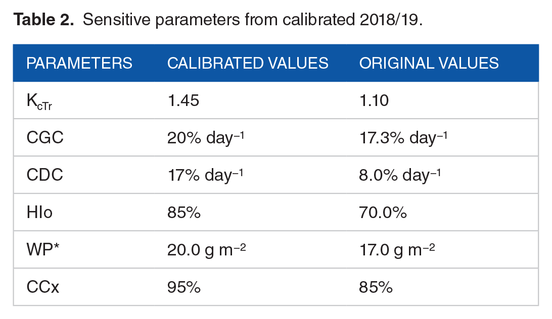
The most important variable in AquaCrop was obtained by sensitivity analysis testing (Geerts et al., 2009; Salemi et al., 2011). The result of the sensitivity of the model (Table 2) shows that the crop transpiration coefficient (K_cTr) when canopy cover is complete, canopy growth coefficient (CGC), canopy decline coefficient (CDC), reference harvest index (HIo), maximum canopy cover (CCx), and normalized water productivity (WP*) had the highest sensitivity. The finding of Afshar and Neshat (2013), who conducted a potato experiment and found that the model is sensitive to the WP* and HIo. Incomparable research by de la Casa et al. (2013) conducted a field experiment to simulate potato crop yield, CCx, CGC, CDC, and WP* are sensitive parameters. In another study, Montoya et al. (2016) performed a field experiment, where the effects of various potato irrigation treatments, the CGC, the CDC, and the WP* are sensitive parameters.

Table 2.

Sensitive parameters from calibrated 2018/19.

Parameters	Calibrated values	Original values
K_cTr	1.45	1.10
CGC	20% day⁻¹	17.3% day⁻¹
CDC	17% day⁻¹	8.0% day⁻¹
HIo	85%	70.0%
WP*	20.0 g m⁻²	17.0 g m⁻²
CCx	95%	85%

Model calibration

The AquaCrop model simulates observed canopy cover, biomass, water use efficiency, irrigation water, and yield for all degrees of water application scenarios. Under the non-limiting condition in the model, the entire 100% irrigation water application scenario was employed to represent crop development. Based on the computed data of full and deficit irrigation water application treatments, the model has been adjusted for the stress condition. The CGC, CDC, and water stress (P_upper, P_lower, and the shape factor) are the key calibrated canopy cover characteristics that determine leaf expansion and early senescence. By setting row and plant spacing, canopy cover per seedling was calculated based on information of the crop parameters. The impacts of the simulation were then correlated with the observed values for the aforesaid crop phenology. Initial canopy cover (CCo) in the model was calculated using data from agronomic procedures such as row and plant spacing of 0.75 and 0.30 m, respectively. As a result, the initial canopy cover estimate for the specified potato crop was found to be 0.22% (4.4 plants m⁻² or 44,444 plants ha⁻¹). The phenological data of the crop criteria stated in Table 3, such as dates of emergency, CCx, senescence, and maturity, were utilized to estimate the canopy expansion rate. As a result of the model, the canopy expands quickly and the canopy declines moderately. The CDC was 17% per day and the CGC was 20% per day, respectively (Table 3). To approximate the recorded canopy cover, stress parameters such as canopy expansion and canopy senescence coefficient were tweaked and readjusted. The obtained harvest index (HI) from the experimental trial of 70% to 85% matches the HIo of 85% (Raes et al., 2012b). This variation was used for fine-tuning for stress conditions, before and during yield formation (Table 3).

Table 3.

Crop parameters and their calibrated model values 2018/19.

Parameters	Unit	Value
Crop phenology
Planting to emergence	DAS	7
Planting to maximum canopy	DAS	50
Planting to start tuber formation	DAS	54
Planting to the maximum depth of rooting	DAS	60
Planting to the beginning of canopy senescence	DAS	85
Planting to maturity	DAS	105
Crop growth and development
Base temperature	°C	10
Upper temperature	°C	30
Planting density	Plants m⁻²	4.4
CCo	%	0.22
CGC	% day⁻¹	20.0
CDC	% day⁻¹	17.0
CCx	%	95
Length to build up of HI	DAS	46
WP*	g m⁻²	20
Water extraction pattern throughout the effective root zone	%	40, 30, 20, 10
Maximum root extraction over the effective root zone	mm day⁻¹	18.0
Crop transpiration coefficient	-	1.45
Canopy shelter in late season	%	60
Maximum rooting depth (m)	Meters	0.6
Shape factor for effective rooting deepening	%	1.5
Yield formation
HIo	%	85
As a result of reduced development in the vegetative cycle, water stress before the onset of yield formation has a favorable impact on HI	-	Strong
Water stress has a positive effect on HI because it affects leaf expansion during yield production	-	Strong
Water stress during yield development has a negative influence on HI due to stomatal closure caused by water stress	-	small
Water stress
The maximum amount of water stress that can cause canopy expansion	-	0.10
The lower threshold for water stress for canopy expansion (P_lower)	-	0.45
The upper limit of the influence of soil water stress on stomatal closure	-	0.45
Early canopy senescence as well as water stress (P_upper)	-	0.55
Waterlogging sensitive to aeration stress	Vol %	8.00

Canopy cover (CC)

Crop parameters were used to model the CC to obtain a good agreement between both the simulated as well as the values of the observed potato crop. Just after the method of calibration, the WP* was calculated as 20.0 g m⁻² (Table 3) and so this value was within the range suggested by Raes et al. (2012b) for C₃ crops (15–20 g m⁻²) and the confidence level defined within the field results. The result of the calibration indicated that the model was capable of simulating CC under different water conditions (Figure 5). In general, the model predicted the seasonal trend in CC as well. However, the model tended to overestimate CC during 80 days after planting in all treatments (Greaves & Wang, 2016). The observed and the simulated CC developments were fitted well for treatment receiving full irrigation throughout the growth stage and were confirmed by the statistical values in Figure 5. The result of this study revealed which model was able to simulate correctly the CC development, but it was seen that the value of CC was overestimated from the senescence to the end of a cropping season in the calibration period 2018/19.

Figure 5.

Calibration of simulated and observed CC.

Montoya et al. (2016) showed the ability of AquaCrop in simulating the CC of the potato crop during the calibration of various water application scenarios. This research is in accordance with other authors (Ngetich et al., 2012) who describe a remarkable match between both the measured and simulated CC on different irrigation treatments. The statistical parameter, coefficient of residual moss having values of negative meant that the model exaggerates the CC. From Figure 5 it is clear that the CC was overstated by the model especially 80, 100 days after sowing, during crop senescence of potato. Pawar et al. (2017), Amirouche et al. (2021) confirmed that the model overestimates CC during the mid-season stage of the crop supported with the CRM value was negative. The calibration was satisfactory as the measured and expected CC values of E ranged from 0.67 to 0.93 at different water application scenarios.

Biomass

The model simulated and measured biomass within full and deficit irrigation conditions (Figure 6). Most of the treatment receiving both irrigation applications shows overestimated biomass at 40, 60, and 80 days after sowing which showed that the CRM’s values were all negative. The finding of Ndambuki (2013), also indicated that the model overestimated the biomass on flowering and maturity of the correctly simulated, while the value of CRM is negative. The treatment delivery of deficit irrigation (T3) described a good fit with the simulated biomass. As seen from Figure 6 the calibrated of deficit irrigation (T3) there was a close association between the observed and predicted biomass. The model was calibrated with model efficiency E of 0.96. This study is in agreement with Greaves and Wang (2016) who identified that the AquaCrop model is a good fit with the measured and simulated biomass of the statistical values of R² = 0.99, RMSE = 1.16, E = 0.97, and d = 0.99 getting deficit irrigation.

Figure 6.

Calibration of simulated and observed biomass.

Overall, the observed and estimated values are in good condition, as shown by the low RMSE, high d, and E values. The value of the statistics mentioned in the current study is similar to those found in other crops. Abedinpour et al. (2012) confirmed that the coefficient of efficiency found that various irrigation treatments were applied between 0.65 and 0.99. The AquaCrop model can be adjusted to simulate potato biomass, yield, and efficiency of water in the study site and becomes a valuable method to help the decision for irrigation purposes.

Harvest index

The value of the harvest index for the different irrigation water application scenarios is derived from the field experiment. For the treatment receiving full irrigation, the harvest index obtained was 0.82. The harvest index values display a decreasing trend under water stress conditions that is 0.81, 0.69, and 0.68 for T3, T2, and T6, respectively. A similar trend was reported by Demelash (2013), Farré and Faci (2009), and Yihun (2015) for potato, maize, sorghum, and teff for water stress conditions. Karunaratne et al. (2011) also reported on Bambara groundnuts in critical growth stages to show a decreasing trend in the harvest index for water stress conditions.

Since soil water stress has a strong impact on the potato harvest index, the effect of soil water stress on different growth stages was recorded and modified in the model. According to the study, water stress prior to flowering has a strong positive impact on the harvest index due to reduced vegetative growth. Water stress during yield formation had a strong positive and small negative impact on harvest index (Table 3) as both a result of water stress affecting leaf expansion and inducing stomatal closure respectively. The result indicates that irrigation application stress at the development and mid-season periods affects potato yield.

Yield, WUE, and irrigation water

The measured potato tuber yields in the field experiment range between 22.89 and 35.15 t ha⁻¹, while the simulated values range between 18.99 and 34.08 t ha⁻¹ (Table 4). The yield deviations reached between −3.02% and −20.53%. The yield reduction mainly occurs when stress is experienced during the potato-sensitive growth stages like development and mid-season. This result is supported by the finding of de la Casa et al. (2013) and Montoya et al. (2016).

Table 4.

Selected parameters of simulated and measured values for calibration period.

Treatment	Yield (t ha⁻¹)			WUE (kg m⁻³)		Dev	IW (mm)		Dev
Treatment	S	M	Dev	S	M	Dev	S	M	Dev
T1	34.08	35.15	−3.14	7.35	8.06	−9.65	483.1	435.80	9.79
T2	19.95	23.29	−16.74	6.12	7.43	−21.40	386.8	326.85	15.49
T3	33.5	34.51	−3.02	8.31	8.78	−5.66	433.1	393.12	9.22
T4	22.01	24.81	−12.72	6.21	7.08	−14.01	404.2	350.45	13.29
T5	26.01	28.88	−11.03	7.15	7.91	−10.62	412.3	364.97	11.47
T6	18.99	22.89	−20.53	6.03	7.31	−21.22	376.7	313.22	16.85

Note. S = simulated; M = measured; Dev = deviation; IW = irrigation water.

The discrepancy in the seasonal water demand between the simulation results and the field measurements for the different irrigation treatments is presented in Table 4. AquaCrop consistently overestimated the seasonal requirements of crop water and the deviations increased as the water deficit increased. The deviations range from 9.22% to 16.85% for the experimental treatments. The study is in accordance with Katerji et al. (2013), who observed that AquaCrop scientifically overestimated the seasonal ETc and the deviations generally increased as stress levels increased. Although the linear regression between simulated and the observed values for all seasons produced an overall R² value of 0.98 the values were relatively distributed, suggesting that model prediction of ETc is fair. As a result of some important mismatch between some of the simulated and actual crop water demand values, the disparity between the calculated and simulated water use efficiency of tuber yields is high for T2 and T6 compared to other deficit treatments (Table 4). The analysis reveals there was no general opinion that the deviations in water use efficiency values were a function of crop water stress. However, the observed efficiency of water use was obviously better in the T3, suggesting that the opportunity for water savings was comparable to that achieved in the full irrigation and other deficit treatments during the planting season for potatoes.

Model validation

The crop parameters that were calibrated were used to validate the model. The validation simulation of the seasonal growth of canopy cover and the accumulation of biomass was carried out during the 2019/20 irrigation season.

Canopy cover (CC)

The data obtained for the 2019/20 irrigation season were used for validation of the model (Figure 7) and show the result of the statistical parameters. The AquaCrop model overestimated the canopy cover during the crop senescence 80 and 100 DAP, in all treatments because of high evapotranspiration during these periods (Figure 7). Due to water stress, the model was insufficient in deficit irrigation at important growth stages (flowering and tuber bulking) since it underestimated comparatively high canopy cover from flowering to harvesting. Similarly, de la Casa et al. (2013) and Greaves and Wang (2016) announced which model overestimated the estimated canopy cover under the water deficit condition of sensitive stages of potato and maize. The validation of critical stages of potato at development and mid-season phases indicates the application of 100% and 75% irrigation water offers good match between the predicted and observed canopy cover of the T3 (Figure 7).

Figure 7.

Validation of simulated and observed CC.

The high values of E and d for the T1 and T3 indicate the overall good agreement between the projected and measured CC. The T6 recorded a high d value of 0.93 but a moderate efficiency value of 0.68. T3 compared to other deficit treatments, showing high model accuracy simulating canopy cover. The test statistics reflect the fitness of the model seen between observed and estimated canopy cover, as shown in (Figure 7). The stress in the development and mid-season phases of the potatoes, as measured and simulated by the coefficient of efficiency, was poor, indicating that the model’s output was acceptable in this level’s stressed condition. During the validation period, the model’s overall performance was overestimated canopy cover, and the coefficient of residual moss value was negative.

Biomass

To validate and calibrate crop parameters for field-grown potato, the biomass obtained at 20 days intervals during the field experiment was compared to the AquaCrop model prediction (Figure 8). There is generally a fair match between the data sets measured and simulation, except for the crop deficit sensitive stages and the 50% deficit in the early and late seasons. Except for the initial stage at 20 days after sowing in all treatments, the model tends to indicate an overestimation of biomass. The model’s efficiency in potato biomass was overestimated, and the value of the residual moss coefficient was negative.

Figure 8.

Validation of simulated and observed biomass.

Yield, efficiency of water use, and irrigation water

Potato yields measured in field experiments ranged from 20.72 to 32.74 t ha⁻¹, while simulated values varied from 16.82 to 31.67 t ha⁻¹ (Table 5). The yield deviation value for the validation period varies between −3.3% and −23.2%. The reduction in potato yield usually occurs when stress occurs during the sensitive growth stages, such as development and mid-season. The above result is in agreement with the finding of de la Casa et al. (2013) and Montoya et al. (2016). For the deficit at critical points, the simulated yield deviation from the observed yield was greater than 12%, signifying that the model accuracy decreases under conditions of extremely stressed water environments. Similar observations were discussed by Evett and Tolk (2009).

Table 5.

Validation parameter of measured and simulated results.

Treatment	Yield (t ha⁻¹)			WUE (kg m⁻³)		Dev	IW (mm)		Dev
	S	M	Dev	S	M	Dev	S	M	Dev
T1	31.67	32.74	−3.4	6.54	7.25	−10.9	478.9	451.6	5.7
T2	17.78	21.12	−18.8	4.92	6.23	−26.6	378.9	339.0	10.5
T3	31.03	32.04	−3.3	7.22	7.69	−6.5	436.9	416.9	4.6
T4	19.82	22.62	−14.1	5.05	5.92	−17.2	415.7	381.9	8.1
T5	23.85	26.72	−12.0	6.09	6.85	−12.5	417.4	390.1	6.5
T6	16.82	20.72	−23.2	5.19	6.47	−24.7	363.7	320.2	12.0

For the various irrigation treatments, the disparity in seasonal crop water between simulation results and measurements was identified in the field experiment. The seasonal crop water requirements were consistently overestimated by AquaCrop, and the deviations grew as the water deficit increased. For the experimental treatments, the variations range from 4.6% to 12% (Table 5). The findings are consistent with those of Katerji et al. (2013), who found that AquaCrop overestimated the seasonal ETc and that the deviations increased as stress levels increased. The gap between measured and simulated water use efficiency of potato yield is high for T2 and T6 as compared to other deficit treatments, due to a significant mismatch between simulated and observed crop water requirement values. However, calculated water use efficiency appeared to be better in the T3, implying the potential for water savings, provided that the yield was comparable to that obtained in the full irrigation during the growing season of potato and other deficit treatments.

Conclusions

Deficit irrigation saves water and improves water productivity while maintaining an optimal yield close to maximum irrigation. This study aimed to evaluate the effects of water shortage on potato production and water use efficiency, as well as to test the AquaCrop model for potato-producing areas of Lasta district. The field experiment showed that 75% and 50% late-season (T6) of the total requirement of crop water indicate higher yield reductions than other deficits irrigation. Taking the above findings into account, it can be concluded that the potato crop has responded positively to mild water stress conditions at our study site. Identifying the sensitive growth stages of a specific cultivar under local weather and soil fertility conditions allows for irrigation scheduling that maximizes crop yield while conserving scarce water. As a result, we discovered that the most vulnerable times for potatoes to be irrigated at 100% ETc were during the development and mid-season periods.

The sensitivity analysis on canopy cover and biomass of calibration treatments showed that Kc_Tr, CGC, CDC, HIo, WP*, and CCx had the highest sensitivity. The findings of this study revealed that AquaCrop can simulate biomass, canopy cover, yield, and water productivity/use efficiency for full supplied irrigation and treatment with some stages of water deficit; however, the model was less satisfactory under water deficit (75% and 50%) at the most important physiological stage of potato compared to the full irrigation at sensitive stages. The highest and lowest accuracy for predicting canopy cover, biomass, yield, and water use efficiencies were obtained at T3 and T6, respectively.

The highest yield of potatoes and water efficiency was found from T3 (33.27 t ha⁻¹) and (8.23 kg m⁻³) by providing 75% ETc during the early and late seasons, while 100% receiving the development and mid-season stages, which is still better than 100% ETc throughout the growing period. As a result, we believe that irrigation water (75%, 100%, 100%, and 75% ETc) is better suited to Lasta district and other similar agro-ecological conditions. This finding could help to improve food security by increasing crop yields and water use efficiency, particularly in areas where water is scarce.

Footnotes

Author Contributions

AW: gathered, analyzed, and interpreted data, as well as writing the paper. MD and HK were in charge of the methodology, as well as the supervision, review, and editing of the paper.

Declaration of Conflicting Interests

The author(s) declared no potential conflicts of interest with respect to the research, authorship, and/or publication of this article.

Funding

The author(s) received no financial support for the research, authorship, and/or publication of this article.

ORCID iD

Hailu Kendie

References

Abdalhi

M. A.

Jia

(2018). Crop yield and water saving potential for aquacrop model under full and deficit irrigation managements. Italian Journal of Agronomy, 13(4), 267–278.

Abedinpour

Sarangi

Rajput

T. B.

Singh

Pathak

Ahmad

(2012). Performance evaluation of AquaCrop model for maize crop in a semi-arid environment. Agricultural Water Management, 110, 55–66.

Afshar

Neshat

(2013). Evaluation of Aqua Crop computer model in the potato under irrigation management of continuity plan of Jiroft region, Kerman, Iran. International Journal of Advanced Biological and Biomedical Research, 1, 1669–1678.

Afsharmanesh

A. A.

Afsharmanesh

G. R.

Adeli

Malekian

(2014). Assessment of aquacrop model in the simulation of potato yield and water use efficiency under different water regimes. Journal of Biological and Environmental Sciences, 8(23), 79–86.

Allen

R. G.

Pereira

L. S.

Raes

Smith

(1998). FAO irrigation and drainage paper no. 56. Food and Agriculture Organization of the United Nations.

Amirouche

Smadhi

Zella

(2021). Calibration and validation of the aquacrop model for the culture lettuce (Lactuca sativa L.) under fertilization levels in pluvial condition. Agricultural Engineering International: CIGR Journal, 23, 36–46.

Bessembinder

J. J.

Leffelaar

P. A.

Dhindwal

A. S.

Ponsioen

T. C.

(2005). Which crop and which drop, and the scope for improvement of water productivity. Agricultural Water Management, 73, 113–130.

Beshir

Kelemu

Birhanu

Ngusie

Endalew

(2018). Performance of improved potato (solanumtuberosum) varieties under irrigation conditions in Wag-Lasta areas of Ethiopia. Proceeding of the 9th and 10th annual regional conference on completed crop research activities, 9–20 March 2015 and 13–16 March 2017, ARARI Bahir Dar, Ethiopia.

Bitri

Grazhdani

Ahmeti

(2014). Validation of the AquaCrop model for full and deficit irrigated potato production in environmental condition of Korça Zone, south-eastern Albania. International Journal of Innovative Research in Science Engineering and Technology, 3, 12013–12020.

10.

Boote

K. J.

Jones

J. W.

Hoogenboom

(1998). Simulation of crop growth: Cropgro model. In Tsuji

G. Y.

Hoogenboom

Thornton

P. K.

(Eds.), Understanding options for agricultural production. Systems approaches for sustainable agricultural development (Vol. 7, pp. 651–692). Springer.

11.

Bradford

Hsiao

(1982). Physiological responses to moderate water stress. In Lange

O. L.

Osmond

P. S.

Ziegler

C. B. H.

(Eds.), Physiological plant ecology II (pp. 263–324). Springer.

12.

Corbari

Ben Charfi

Mancini

(2021). Optimizing irrigation water use efficiency for tomato and maize fields across Italy combining remote sensing data and the AquaCrop model. Hydrology, 8, 39.

13.

CSA. (2019). Agricultural sample survey 2018/19. Volume I. Report on area and production of major crops for private peasant holdings, meher season. Statistical Bulletin 589, Central Statistical Agency, Addis Ababa, Ethiopia.

14.

de la Casa

Ovando

Bressanini

Martínez

(2013). Aquacrop model calibration in potato and its use to estimate yield variability under field conditions. Atmospheric and Climate Sciences, 03, 397–407.

15.

Demelash

(2013). Deficit irrigation scheduling for potato production in North Gondar, Ethiopia. African Journal of Agricultural Research, 8, 1144–1154.

16.

Demelash

Alamirew

(2011). Deficit irrigation scheduling for potato production in north Gondar zone, Ethiopia. MSc thesis, Haramaya University.

17.

Deressa

T. T.

Hassan

R. M.

Ringler

Alemu

Yesuf

(2009). Determinants of farmers’ choice of adaptation methods to climate change in the Nile Basin of Ethiopia. Global Environmental Change, 19, 248–255.

18.

Domínguez

de Juan

J. A.

Tarjuelo

J. M.

Martínez

R. S.

Martínez-Romero

(2012). Determination of optimal regulated deficit irrigation strategies for maize in a semi-arid environment. Agricultural Water Management, 110, 67–77.

19.

Eitzinger

Trnka

Hösch

Žalud

Dubrovský

(2004). Comparison of CERES, WOFOST and SWAP models in simulating soil water content during growing season under different soil conditions. Ecological Modelling, 171, 223–246.

20.

Evett

S. R.

Tolk

J. A.

(2009). Introduction: Can water use efficiency be modeled well enough to impact crop management? Agronomy Journal, 101, 423–425.

21.

Fabeiro

Martı́n de Santa Olalla

de Juan

J. A.

(2001). Yield and size of deficit irrigated potatoes. Agricultural Water Management, 48, 255–266.

22.

Farré

Faci

J. M.

(2009). Deficit irrigation in maize for reducing agricultural water use in a Mediterranean environment. Agricultural Water Management, 96, 383–394.

23.

Fereres

Soriano

M. A.

(2007). Deficit irrigation for reducing agricultural water use. Journal of Experimental Botany, 58, 147–159.

24.

Foster

Brozovic

Butler

A. P.

Neale

C. M.

Raes

Steduto

Fereres

Hsiao

T. C.

(2017). AquaCrop-OS: A tool for resilient management of land and water resources in agriculture [Conference session]. EGU General Assembly Conference Abstracts (p. 2842).

25.

Gebremedhin

Berhe

Nebiyu

(2015). Performance of AquaCrop model in simulating tuber yield of potato (Solanum tuberosum L.) under various water availability conditions in Mekelle area, northern Ethiopia. Journal of Natural Sciences Research, 5, 123–130.

26.

Gebreselassie

Ayana

Tadele

(2015). Field experimentation based simulation of yield response of maize crop to deficit irrigation using AquaCrop model, Arba Minch, Ethiopia. African Journal of Agricultural Research, 10, 269–280.

27.

Geerts

Raes

(2009). Deficit irrigation as an on-farm strategy to maximize crop water productivity in dry areas. Agricultural Water Management, 96, 1275–1284.

28.

Geerts

Raes

Garcia

Miranda

Cusicanqui

J. A.

Taboada

Mendoza

Huanca

Mamani

Condori

Mamani

Morales

Osco

Steduto

(2009). Simulating yield response of quinoa to water availability with AquaCrop. Agronomy Journal, 101, 499–508.

29.

Greaves

Wang

Y.-M.

(2016). Assessment of FAO AquaCrop model for simulating maize growth and productivity under deficit irrigation in a tropical environment. Water, 8, 557.

30.

Hsiao

T. C.

Heng

Steduto

Rojas-Lara

Raes

Fereres

(2009). AquaCrop the FAO crop model to simulate yield response to water: III. Parameterization and testing for maize. Agronomy Journal, 101, 448–459.

31.

Heng

L. K.

Hsiao

Evett

Howell

Steduto

(2009). Validating the FAO AquaCrop model for irrigated and water deficient field maize. Agronomy Journal, 101, 488–498.

32.

Hirpa

Meuwissen

M. P. M.

Tesfaye

Lommen

W. J. M.

Oude Lansink

Tsegaye

Struik

P. C.

(2010). Analysis of seed potato systems in Ethiopia. American Journal of Potato Research, 87, 537–552.

33.

Ierna

Mauromicale

(2012). Tuber yield and irrigation water productivity in early potatoes as affected by irrigation regime. Agricultural Water Management, 115, 276–284.

34.

Kale

(2016). Assessment of AQUACROP model in the simulation of wheat growth under different water regimes. Scientific Papers-Series A, Agronomy, 59, 308–314.

35.

Karunaratne

A. S.

Azam-Ali

S. N.

Izzi

Steduto

(2011). Calibration and validation of FAO-AquaCrop model for irrigated and water deficient bambara groundnut. Experimental Agriculture, 47, 509–527.

36.

Kashyap

P. S.

Panda

R. K.

(2003). Effect of irrigation scheduling on potato crop parameters under water stressed conditions. Agricultural Water Management, 59, 49–66.

37.

Katerji

Campi

Mastrorilli

(2013). Productivity, evapotranspiration, and water use efficiency of corn and tomato crops simulated by AquaCrop under contrasting water stress conditions in the Mediterranean region. Agricultural Water Management, 130, 14–26.

38.

Mibulo

Kiggundu

(2018). Evaluation of FAO AquaCrop model for simulating rainfed maize growth and yields in Uganda. Agronomy, 8, 238.

39.

Montoya

Camargo

Ortega

J. F.

Córcoles

J. I.

Domínguez

(2016). Evaluation of aquacrop model for a potato crop under different irrigation conditions. Agricultural Water Management, 164, 267–280.

40.

Nash

J. E.

Sutcliffe

J. V.

(1970). River flow forecasting through conceptual models part I — A discussion of principles. Journal of Hydrology, 10, 282–290.

41.

Ndambuki

(2013). Application of AquaCrop model in deficit irrigation management of cabbages in Keiyo Highlands. International Journal of Water Resources and Environmental Engineering, 5, 360–369.

42.

Ngetich

Raes

Shisanya

Mugwe

Mucheru-Muna

Mugendi

Diels

Books

Sheets

Oer

(2012). Calibration and validation of AquaCrop model for maize in sub-humid and semi-arid regions of central highlands of Kenya [Conference session]. RUFORUM Third Biennial Conference, Entebbe, Uganda (pp. 24–28).

43.

Onder

Caliskan

M. E.

Onder

Caliskan

(2005). Different irrigation methods and water stress effects on potato yield and yield components. Agricultural Water Management, 73, 73–86.

44.

Pawar

G. S.

Kale

M. U.

Lokhande

J. N.

(2017). Response of AquaCrop model to different irrigation schedules for irrigated cabbage. Agricultural Research, 6, 73–81.

45.

Raes

Steduto

Hsiao

Fereres

(2012a). Aquacrop reference manual. FAO, Land and Water Division.

46.

Raes

Steduto

Hsiao

Fereres

(2012b). Reference manual AquaCrop (Version 4.0). AquaCrop. http://www.fao.org/nr/water/aquacrop.html

47.

Razzaghi

Zhou

Andersen

M.N.

Plauborg

(2017). Simulation of potato yield in temperate condition by the aquacrop model. Agricultural Water Management, 191, pp.113-123.

48.

Salemi

Soom

M. A. M.

Lee

T. S.

Mousavi

S. F.

Ganji

KamilYusoff

(2011). Application of AquaCrop model in deficit irrigation management of winter wheat in arid region. African Journal of Agricultural Research, 6, 2204–2215.

49.

Saxton

K. E.

Rawls

W. J.

(2006). Soil water characteristic estimates by texture and organic matter for hydrologic solutions. Soil Science Society of America Journal, 70, 1569–1578.

50.

Shahnazari

Liu

Andersen

M. N.

Jacobsen

S.-E.

Jensen

C. R.

(2007). Effects of partial root-zone drying on yield, tuber size and water use efficiency in potato under field conditions. Field Crops Research, 100(1), 117–124.

51.

Shock

C. C.

Feibert

E. B.

Saunders

L. D.

(1998). Potato yield and quality response to deficit irrigation. HortScience, 33, 655–659.

52.

Smith

(2000). The application of climatic data for planning and management of sustainable rainfed and irrigated crop production. Agricultural and Forest Meteorology, 103, 99–108.

53.

Soomro

K. B.

Alaghmand

Shahid

M. R.

Andriyas

Talei

(2020). Evaluation of AquaCrop model in simulating bitter gourd water productivity under saline irrigation. Irrigation and Drainage, 69, 63–73.

54.

Steduto

Hsiao

Fereres

Raes

(2012). Crop yield response to water (FAO Irrigation and Drainage Paper No. 66). Food and Agriculture Organization of the United Nations.

55.

Tefera

A. H.

Mitiku

D. T.

(2021). Models comparative study for estimating crop water requirement and irrigation scheduling of maize in Metekel Zone, Benishangul Gumuz Regional State, Ethiopia. International Journal of Agricultural Economics, 6, 59.

56.

Vos

Haverkort

(2007). Water availability and potato crop performance. In Vreugdenhil

(Ed.), Potato biology and biotechnology (pp. 333–351). Elsevier.

57.

Willmott

Matsuura

(2005). Advantages of the mean absolute error (MAE) over the root mean square error (RMSE) in assessing average model performance. Climate Research, 30, 79–82.

58.

Yihun

Y. M.

(2015). Agricultural water productivity optimization for irrigated Teff (Eragrostic Tef) in water scarce semi-arid region of Ethiopia. CRC Press/Balkema.

Evaluating the Performance of AquaCrop Model for Potato Production Under Deficit Irrigation

Abstract

Keywords

Introduction

Material and Methods

Study area description

Treatment and experimental design

Water requirement of potato

AquaCrop model input data

Climate data

Crop parameters

Soil characteristics

Irrigation and field management

Model calibration

Model validation

Model evaluation

Result and Discussion

Soil properties

Aquacrop model sensitivity

Model calibration

Canopy cover (CC)

Biomass

Harvest index

Yield, WUE, and irrigation water

Model validation

Canopy cover (CC)

Biomass

Yield, efficiency of water use, and irrigation water

Conclusions

Footnotes

Author Contributions

Declaration of Conflicting Interests

Funding

ORCID iD

References