Sage Journals: Discover world-class research

Abstract

We review simple methods for evaluating 4 types of biomarkers. First, we discuss the evaluation of surrogate endpoint biomarkers (to shorten a randomized trial) using 2 statistical and 3 biological criteria. Second, we discuss the evaluation of prognostic biomarkers (to predict the risk of disease) by comparing data collection costs with the anticipated net benefit of risk prediction. Third, we discuss the evaluation of predictive markers (to search for a promising subgroup in a randomized trial) using a multivariate subpopulation treatment effect pattern plot involving a risk difference or responders-only benefit function. Fourth, we discuss the evaluation of cancer screening biomarkers (to predict cancer in asymptomatic persons) using methodology to substantially reduce the sample size with stored specimens.

Keywords

Decision curve net benefit relative utility curve risk prediction risk-based decision-making

Introduction

The National Institutes of Health (NIH) Biomarkers Definitions Working Group defined a biomarker as “a characteristic that is objectively measured and evaluated as an indicator of normal biological processes, pathogenic processes, or pharmacologic responses to a therapeutic intervention.”¹ Examples of biomarkers are changes in genes, proteins, cells, or tissue, or physiological measurements such a blood pressure. This article reviews simple methods for evaluating 4 types of biomarkers defined by their use: surrogate endpoint biomarker to shorten randomized trials, prognostic biomarkers to predict the risk of disease, predictive biomarkers to search for a promising subgroup in a randomized trial, and cancer screening biomarkers to predict cancer in asymptomatic persons.

Surrogate Endpoint Biomarkers to Shorten Randomized Trials

When a randomized trial requires a long time to obtain a true (clinically meaningful) endpoint, investigators are often interested in evaluating treatment effect sooner using a surrogate endpoint biomarker (also called a response biomarker).² A surrogate endpoint biomarker is a biomarker observed after randomization and before the true endpoint that is used to draw conclusions about the effect of treatment on the true endpoint. For example, some investigators have considered prostate-specific antigen (PSA) as a surrogate endpoint biomarker for symptomatic prostate cancer.³ The use of a surrogate endpoint biomarker (also called a surrogate endpoint) is fundamentally an exercise in extrapolation,⁴ with the strong possibility of obtaining misleading results.⁵ Therefore, before its use to shorten a randomized trial, a surrogate endpoint must satisfy stringent criteria, in order to be considered clinically validated.

Problematic criteria for a surrogate endpoint

Many commonly used criteria for evaluating a surrogate endpoint can yield incorrect or uninformative results. For a valid surrogate endpoint, the Prentice Criterion⁶ requires that the probability of the true endpoint given the surrogate endpoint is the same in each randomization group. This requirement implies a single pathway from treatment to true outcome that passes through the surrogate outcome. The main problem with using the Prentice Criterion is that it requires a detailed understanding of the biological pathway, and such detailed knowledge is typically lacking. Moreover, in a small surrogate endpoint trial corresponding to a true endpoint that would require a large trial for adequate power, even a small deviation from the Prentice criterion can invalidate the surrogate endpoint.⁷ Another commonly used criterion is a high proportion of treatment effect explained by the surrogate endpoint. Its major drawback is that the confidence intervals are typically too wide to be informative.^8,9 A third commonly used criterion for evaluating a surrogate endpoint is a high correlation between surrogate and true endpoints within each arm of the trial. However, this criterion provides little or no information for using a surrogate endpoint to draw conclusions about the effect of treatment on a true endpoint. Even perfect correlation between surrogate and true endpoints within each arm does not guarantee correct conclusions about the effect of treatment on true endpoint.¹⁰

Meta-analytic surrogate endpoint evaluation

For evaluating surrogate endpoints, many statisticians favor criteria based on data from multiple historical trials with surrogate and true endpoints. In this context, a frequently used criterion is a high trial-level association between the estimated effect of treatment on the surrogate endpoint and the estimated effect of treatment on the true endpoint.^11-13 The limitation of this criterion is the difficulty of determining the threshold for acceptability of the surrogate endpoint.¹⁴ A useful supplement to the trial-level correlation is the surrogate threshold effect, the minimum effect of treatment on the surrogate endpoint necessary to predict a statistically significant effect of treatment on the true endpoint.¹⁴

Five simple criteria for meta-analytic surrogate endpoint evaluation

A simple approach to the evaluation of surrogate endpoints from historical trials involves 5 criteria, 2 of which are statistical, and 3 of which are biological.¹⁵ The 2 statistical criteria arise from a random effects zero-intercept linear regression of the estimated effect of treatment on true endpoint as a function of the estimated effect of treatment on the surrogate endpoint. The random effects component captures the variability in the effect of treatment on the true endpoint, which can vary considerably among different treatments and study settings. The zero intercept in the regression has 2 desirable properties. First, it ensures that a zero effect of treatment on the surrogate endpoint implies a zero effect of treatment on the true endpoint. Second, it ensures that changing the labels of control and experimental treatment does not change the model.^16,17 For example, when comparing treatments A and B in one trial, B and C in another trial, and A and C in a third trial, it is not clear which treatments are control treatments and which are experimental treatments, so a model for the estimated effect of treatment on true endpoint, given the estimated effect of treatment on the surrogate endpoint should be invariant to the labeling of control and experimental treatments. See Figure 1 based on the hypothetical data in Table 1 for an example of the zero-intercept random-effects linear regression. See Appendix 1 for mathematical details.

Figure 1.

Surrogate endpoint meta-analysis for hypothetical data. The plot is based on the data in Table 1 and shows a zero-intercept random-effects linear regression (solid blue line) with 95% prediction band (dashed blue lines). Vertical black lines are 95% confidence intervals for the estimated effect of treatment on the predicted endpoint.

Table 1.

Hypothetical data for a surrogate endpoint meta-analysis. Based on formulas in Appendix 1, the sample size multiplier is 1.61 and the prediction separation score is 1.18.

Sample size per arm	Estimated effect of treatment on surrogate endpoint	Estimated effect of treatment on true endpoint	Standard error of estimated effect of treatment on true endpoint
43	0.19	3.5	3.8
79	1.16	−2.2	1.1
44	1.81	6.2	2.6
66	2.63	7.2	1.7
51	4.03	13.6	4.0
31	5.19	24.8	4.1

Below is a list of 5 criteria for the acceptable use of a surrogate endpoint in a new trial when applying the zero-intercept random-effects model to data from historical trials with both surrogate and true endpoints. The first 2 criteria are statistical and relate directly to the model. The last 3 involve biological and clinical considerations when extrapolating to a new trial.

Criterion 1. An acceptable sample size multiplier

The sample size multiplier is the sample size for the predicted effect of treatment on the true endpoint based on the surrogate endpoint divided by the sample size for the observed effect of treatment on the true endpoint (evaluated at the median effect of treatment on the surrogate endpoint). The sample size multiplier is greater than 1 because prediction involves more variability than the direct observation. Investigators use the sample size multiplier to decide if the larger sample size needed with a surrogate endpoint is worth the benefit of shortening the trial duration by using the surrogate endpoint.

Criterion 2. A prediction separation score larger than 1

The prediction separation score is the maximum change in the predicted treatment effect over the historical trials divided by the width of the prediction band at the median effect of treatment on the surrogate endpoint. A prediction separation score larger than 1 indicates no overlap of prediction bands at the extreme values for the range of surrogate endpoints in the historical trials, a strong indicator that the effect of treatment on the surrogate endpoint is informative for the effect of treatment on the true endpoint.

Criterion 3. Similarity of biological mechanism of treatments in the new trial and the historical trials

If the new trial evaluates a treatment with a novel mechanism, it is doubtful that application of a surrogate endpoint from historical trials would be relevant to the new trial.¹⁸ Hence, this criterion is necessary for extrapolating from historical trials to the new trial involving only the surrogate endpoint.

Criterion 4. Similarity of secondary treatments following the observation of the surrogate endpoint

If the new trial involved a novel secondary treatment prompted by the surrogate endpoint, the surrogate endpoint evaluation based on previous trials would not apply.

Criterion 5. A low risk of harmful side effects after observation of the surrogate endpoint

Even if the effect of treatment on the surrogate endpoint correctly predicted the effect of treatment on the true endpoint, use of the surrogate endpoint in a new trial is problematic if sufficiently harmful side effects (outweighing the benefits) arise after the time the surrogate endpoint is observed.¹⁸ Of course, investigators would not know if there were harmful late-occurring side effects at the time when a trial is stopped to measure the surrogate endpoint, but they should consider this possibility based on their knowledge of the new treatment.

These criteria represent an appropriately high bar for evaluating trials involving a surrogate endpoint that are designed to change practice. For a preliminary exploratory study, such a high bar may not be needed, so investigators could relax some of these criteria. The main practical limitation of any method to evaluate surrogate endpoints is an incomplete understanding of the biology linking surrogate and true endpoints.

Prognostic Biomarkers to Improve Risk Prediction

Prognostic biomarkers² (also called risk prediction biomarkers) predict the development of disease or a clinical event with the goal of making treatment decisions. In many situations, investigators compare 2 risk prediction models in a validation sample:

Model 1 based on standard predictors.

Model 2 based on the standard predictors and prognostic biomarkers.

The validation sample should be a random sample of persons from a target population, possibly stratified by cases (who develop disease) and controls (who do not develop disease) in a nested case–control design. The goal is to draw conclusions about the prediction performance of Model 2 versus Model 1 in the target population.

Consider predicting the risk of invasive breast cancer in asymptomatic women. Women at sufficiently high risk receive treatment to reduce the risk of invasive breast cancer. Such treatment would likely be associated with harmful side effects. Model 1 was a risk-prediction model based on a questionnaire about risk factors including age and family history. Model 2 was based on the same questionnaire as Model 1 with the addition of information on single nucleotide polymorphisms (SNPs).¹⁹

If there were no costs or harm to collecting data on prognostic markers and the added prognostic markers were statistically significant, investigators would base risk prediction on Model 2 instead of Model 1. However, there is often a monetary cost or a harm associated with collecting data on the prognostic markers. For example, collecting information on SNPs has a monetary cost. Therefore, investigators need to weigh the cost of collecting data on the prognostic biomarker versus the anticipated benefits and harms of improved risk prediction.

The limitation of purely statistical measures

Standard statistical measures for comparing the performance of Models 1 and 2, such as the change in the area under the receiver operating characteristic (ROC) curve (AUC)²⁰ and the net reclassification improvement,²¹ provide limited information for evaluating prognostic biomarkers because they do not account for the data collection costs or the benefits and harms of treatment. Another drawback of the net reclassification improvement is that it can give misleading results when the new biomarker has no predictive value.²²

A simple decision-analytic evaluation

Decision analysis provides a framework for comparing Models 1 and 2, which incorporates data collection costs and harms and benefits of treatment. Methodology involving decision curves^23-25 or relative utility curves^26-28 provides a sensitivity analysis based on varying the risk threshold, which is the risk of disease at which a person would be indifferent between treatment and no treatment. A useful statistic developed with relative utility curves is the test tradeoff, which is the minimum number of data collections per true positive to yield a positive net benefit.^27,28 Computation of the test tradeoff can be challenging. However, using AUC’s from Models 1 and 2, investigators can easily approximate the minimum test tradeoff (MTT) as

MTT = \frac{1}{{(h (AU C_{2}) - h (AU C_{1})} \times P}

where

h (AUC) = AUC - {\frac{1 - AUC}{2}}^{\frac{1}{2}}

AU C_{1} = AUC for Model 1,

AU C_{2} = AUC for Model 2,

\begin{array}{l} P = probability of developing disease in \\ the target population \end{array}

The MTT is useful for ruling out a risk-prediction model. In the study of the 5-year risk of invasive breast cancer, AUC₁ = 0.56 and AUC₂ = 0.59. For P = .003, the MTT = 1/({h[0.59]—h[0.56]} × 0.003) = 7200. Thus, at least 7200 sets of SNPs would be needed for every true positive to yield a positive net benefit in this example. If the MTT of 7200 is unacceptable, the MTT would rule out Model 2 in this example.

A practical limitation with the decision curves or relative utility curves is the difficulty of specifying a range of risk thresholds (indicating acceptable cost–benefit tradeoffs) because the benefit of treatment is typically unknown. However, for the more limited goal of ruling out a risk prediction model with MTT, which does not involve a range of risk thresholds, this limitation is not a concern.

Predictive Biomarkers to Identify a Promising Subgroup in Randomized Trials

Predictive biomarkers (also called treatment selection markers)²⁹ are baseline biomarkers in a randomized trial that are used to identify a subgroup in randomized trial with an estimated treatment effect that is larger than the overall estimated treatment effect for the entire trial. A subgroup analysis is particularly useful when the estimated treatment effect in the subgroup is statistically significant and sufficiently large to outweigh any harms of treatment while the estimated overall treatment effect for the entire trial is not statistically significant.

Limitations of standard approaches with treatment-marker interactions

The standard approach to subgroup analysis involves modeling outcome as a function of randomization group with a term for the interaction between treatment assignment and biomarker.^29-31 This standard approach has 2 limitations. First, the interaction lacks a direct clinical interpretation of the usefulness of the marker for treatment selection.³² Second, this approach does not parsimoniously combine information from multiple markers, complicating estimation and interpretation.

A simple implementation using multivariate STEPP

A simple and informative method for using predictive markers in a subgroup analysis involves a multivariate version of the subpopulation treatment effect pattern plot (STEPP).³³ The original STEPP graphed estimated treatment effect in a subgroup versus a single predictive marker.^34,35 A multivariate STEPP graphs the estimated treatment effect in a subgroup versus a benefit score derived from a combination of markers. A general approach to mitigating problems with reproducibility in multivariate analyses is to separate model fitting from model evaluation. To implement a multivariate STEPP, investigators randomly split the data in a randomized trial into training and test samples, with model fitting in the training sample and subgroup selection and evaluation in the test sample.

Using the training sample, investigators fit a benefit function based on a set of predictive markers. The risk difference benefit function (called a single index scoring system³⁶ or a single index score³⁷ in related approaches) is the predicted difference in favorable outcomes between randomization groups as a function of the predictive markers. Mathematically, the risk difference benefit function has the form

\begin{array}{l} RiskDifference (x) = pr (Y = 1 | new treatment, x) \\ - pr (Y = 1 | old treatment, x), \end{array}

where Y is outcome, Y = 1 is a favorable outcome, and x is a list of biomarkers. For the risk difference benefit function, investigators can fit a separate logistic regression to each randomization group.

The responders-only benefit function (independently formulated as a marker-specific treatment effect model in a case-only approach)³⁸ is the estimated probability of assignment to the new treatment among participants with a rare outcome as a function of the predictive markers. Mathematically, the responders-only benefit function has the form,

ResponderOnly (x) = \frac{pr (new treatment | Y = 1, x)}{pr (old treatment | Y = 1, x)}

where Y = 1 is the rare outcome that identifies “responders.” For the responders-only benefit function, investigators can fit a single regression model to an indicator of new versus old treatment. The responders-only benefit function can be equivalently written as ResponderOnly(x) = 1 + RiskDifference(x)/pr(Y = 1|old treatment, x), indicating that it is a function of the risk difference benefit function, and thereby not introducing bias by focusing only on responders. For a rare outcome, the responders-only benefit function substantially reduces data collection costs relative to the risk difference benefit function because investigators need only measure the marker in participants with the rare outcome.

For each participant in the test sample, investigators compute a benefit score s by applying the benefit function to the participants’ predictive markers. Let d denote the difference in the estimated probabilities of a favorable outcome between randomization groups among participants with a benefit score greater than or equal to s. The multivariate STEPP plots d and its 95% confidence band versus the benefit score s. To simplify computations, investigators can consider 5 benefit score cutpoints at quantiles ranging from a small value to 1 and, using a Bonferroni adjustment, compute 1 – .025/5 = 99.5% confidence intervals (estimate ±2.58 × standard error) at each cutpoint. A more complicated adjustment for multiple comparisons could use a simulation to obtain a narrower confidence band.³³

For an example of a multivariate STEPP with artificial data, see Table 2 and the corresponding Figure 2. In Table 2, the estimated overall treatment effect for the entire trial, which corresponds to Quantile 1.00 and benefit score −0.96, is not statistically significant, while the estimated treatment effect in the subgroup defined by quantile 0.50 and benefit score −1.95 is statistically significant after adjustment for multiple comparisons.

Table 2.

Hypothetical data for computing multivariate STEPP, which plots d versus s. The 95% confidence bands plot d_LOW versus s and d_UPP versus s.

	Benefit score s
Benefit score	−0.96	−0.577	−0.195	0.188	0.57
Approximate quantile	1.00	0.81	0.50	0.24	0.07
x₀ = number in randomization group 0 with benefit score ⩾s and a favorable outcome	159	124	74	34	6
x₁ = number in randomization group 1 with benefit score ⩾s and a favorable outcome	134	128	94	50	19
n₀ = number in randomization group 0 with benefit score ⩾s	300	241	155	76	21
n₁ = number in randomization group 1 with benefit score ⩾s	300	247	147	67	20
d = p₁ – p₀, where p_j = x_j/n_j	−0.083	0.004	0.162	0.299	0.664
se = {p₁(1 – p₁)/n₁ + p₀(1 – p₀)/n₀}^1/2	0.041	0.045	0.056	0.078	0.11
d_LOW = d – 2.58se	−0.188	−0.113	0.017	0.098	0.381
d_UPP = d + 2.58se	0.021	0.12	0.307	0.5	0.948

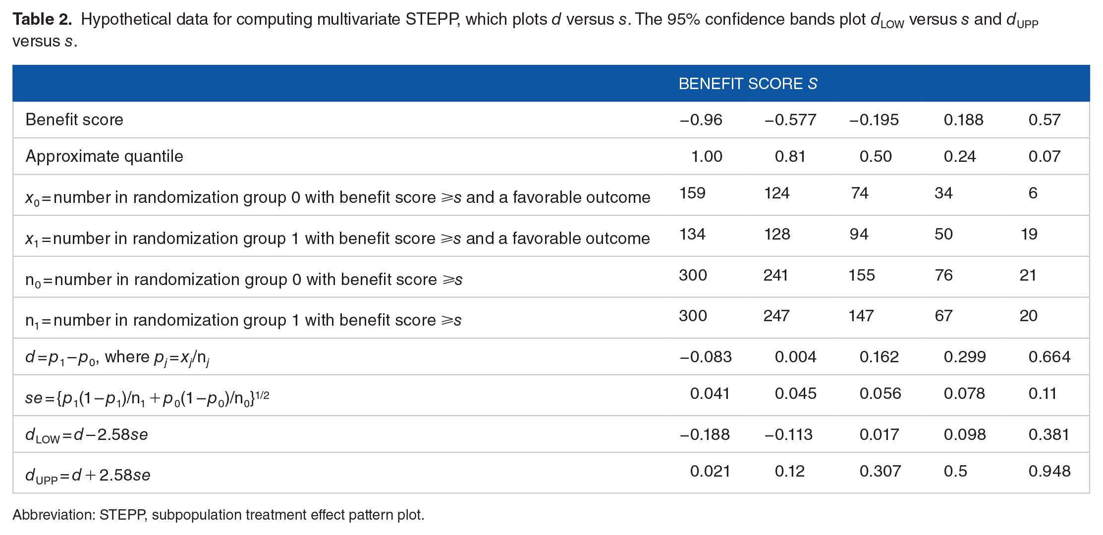
Abbreviation: STEPP, subpopulation treatment effect pattern plot.

Figure 2.

Multivariate STEPP for hypothetical data. The plot is based on the data in Table 2. The dashed line indicates the 95% confidence band. STEPP indicate subpopulation treatment effect pattern plot.

The main practical limitation of this methodology is that it can only detect a large subgroup treatment effect because of the reduced sample size resulting from the split into training and test samples with further restriction to the subgroup in the test sample and adjustment for multiple comparisons. Nevertheless, if data on predictive markers are readily available, the multivariate STEPP is worth applying on the chance of finding a large subgroup treatment effect.

Cancer Screening Biomarkers to Predict Cancer in Asymptomatic Persons

Cancer screening is the testing of persons asymptomatic for cancer for the presence of precancerous lesions, early-stage cancer or cancer screening biomarkers, followed by early intervention if the test is positive.³⁹ A cancer screening biomarker (also called a marker for the early detection of cancer) is a prognostic biomarker that predicts the development of symptomatic cancer in asymptomatic persons. In practice, investigators combine cancer screening markers into a cancer prediction model. The main stages in the biomarker pipeline to develop and evaluate cancer screening tests are (1) discovery of new cancer screening biomarkers (ideally from stored specimens in asymptomatic persons) and their combination into a cancer prediction model, (2) validation of the cancer prediction model using stored specimens from asymptomatic persons, (3) initial short-term evaluation of cancer screening biomarkers as triggers of early intervention, and (4) the definitive long-term evaluation of cancer screening biomarkers as triggers of early intervention using a large randomized trial with a cancer mortality endpoint.³⁹ This pipeline differs from the more commonly discussed phases of biomarker development for cancer screening tests⁴⁰ in the ideal use stored specimens for discovery and the different short-term evaluations of cancer screening biomarkers as triggers of early intervention (such as the application of the paired availability design^41,42 to an interval cancer endpoint).

The focus of this discussion is the validation of cancer prediction models using stored specimens. In a typical validation study, investigators collect stored specimens from asymptomatic persons, follow the participants a few years, and ascertain the biomarkers from the stored specimens in all persons who develop symptomatic cancer and a random sample who do not.⁴³ A major obstacle to implementing this biomarker validation study is the large sample size, which is a consequence of the low cancer incidence among the asymptomatic participants.

A key goal in the evaluation of cancer screening biomarkers is to reduce the validation sample size while increasing prediction performance. To achieve this goal, it is necessary to consider 2 pairs of performance metrics. One pair of performance metrics is sensitivity, the probability of a positive prediction, given a person later develops cancer, and specificity, the probability of a negative prediction given a person does not later develop cancer. Another pair of performance metrics is positive predictive value, the probability of developing cancer, given a positive prediction, and the negative predictive value, the probability of not developing cancer, given a negative prediction. In this application, sensitivity and specificity determine sample size, while positive predictive and negative predictive values provide a more interpretable measure of prediction performance. As incorrect prediction of cancer can lead to unnecessary and sometimes harmful early interventions, the positive predictive value needs to be as large as possible. For the rare outcome of symptomatic cancer during the study period, the negative predictive value is approximately equal to 1, and a large positive predictive value requires a very high specificity regardless of the sensitivity.⁴⁴ The following discussion compares standard and revised target performances for sensitivity and specificity and their implications for positive predictive value. In the discussion, lower bound refers to 2.5%.

Sample size based on a standard target performance

A standard target performance for a validation study of cancer screening biomarkers is a sensitivity of 80% with a lower bound of 70% sensitivity and a specificity of 99% with a lower bound of 97% specificity.^43,45,46 As discussed in Appendix 2, the standard target performance translates into intermediate sample sizes of 70 cases and 300 controls. If the probability of developing cancer in the study is 1%, the validation sample size needed to achieve the intermediate sample sizes is 8600 participants with stored specimens, and the lower bound on the positive predictive value is 0.19.

Substantially reduced sample size based on the revised target performance

The key to reducing sample size while improving the positive predictive value is to change from the standard target performance to the revised target performance that involves an imprecise sensitivity and a precise perfect specificity.^45,46 The revised target performance specifies either a sensitivity of 80% with a lower bound of 50% sensitivity under Scenario 1 or a sensitivity of 50% with a lower bound of 20% sensitivity under Scenario 2. It also specifies a specificity of 100% with a lower bound of 99.5% specificity. As discussed in Appendix 2, the revised target performance translates into intermediate sample sizes of 12 cases and 740 controls. If the probability of developing cancer in the study is 1%, the validation sample size needed to achieve the intermediate sample sizes is 2000 persons, and the lower bound on the positive predictive value is 0.29 under Scenario 1 and 0.50 under Scenario 2. Thus, relative to the standard target performance, the revised target performance both reduces sample size and increases the lower bound on the positive predictive value. Importantly, the reduced sample size can make some otherwise infeasible validation studies feasible. Table 3 shows the validation sample sizes and lower bounds on the positive predictive values under both standard and revised target performances.

Table 3.

Validation sample sizes and lower bounds on the positive predictive value with standard and revised target performances.

Probability of developing cancer in the population	Standard target performanceSensitivity = 80% (LB = 70%).Specificity = 99% (LB = 97%).		Revised target performanceSensitivity = 50% (LB = 20%) for Scenario 1.Sensitivity = 80% (LB = 50%) for Scenario 2.Specificity = 100% (LB = 99.5%).
	Validation sample size	PPV lower bound	Validation sample size	PPV lower bound
	Validation sample size	PPV lower bound	Validation sample size	Scenario 1	Scenario 2
0.005	17 100	0.10	3900	0.17	0.33
0.007	12 200	0.14	2800	0.22	0.41
0.010	8600	0.19	2000	0.29	0.50
0.015	5700	0.26	1300	0.38	0.60
0.020	4300	0.32	1000	0.45	0.67
0.025	3500	0.37	800	0.51	0.72

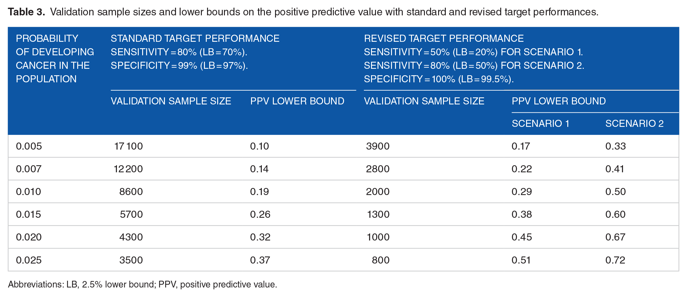
Abbreviations: LB, 2.5% lower bound; PPV, positive predictive value.

The double-dip design

The reduction in the validation sample size with the revised target performance is the basis for the double-dip design, which makes biomarker discovery more relevant.⁴⁶ The problem with standard biomarker discovery is that it is usually based on a convenience sample of biomarkers collected from persons with symptomatic cancer and from controls without clinical cancer. Biomarkers identified from a convenience sample may have little relevance for cancer prediction among asymptomatic persons.⁴⁶ The double-dip design begins with standard biomarker discovery using a convenience sample. If the cancer prediction model derived from the convenience sample performs poorly in the validation sample of stored specimens from asymptomatic persons, the double-dip design uses the validation sample of stored specimens for second-chance discovery (the double dip) followed by a second validation sample of stored specimens. The practical limitation of the double-dip design is the limited sample size of the more relevant discovery sample involving stored specimens. However, this limitation is outweighed by the benefit of more relevant second-chance discovery.

Discussion

The focus here is on methods of biomarker evaluation that have a solid conceptual basis and are relatively easy to implement compared with some other approaches in the literature. The zero-intercept random-effects model for the meta-analytic surrogate endpoint evaluation is easy to compute using the formulas in Appendix 1. For prognostic and predictive biomarkers, it is necessary to fit a model to predict the binary outcome based on multiple biomarkers. Investigators often use a logistic regression model for prediction, which often performs as well as more complicated machine learning algorithms.⁴⁷ However, investigators can also use machine-learning algorithms. Once the models are fit, the next step is to find the appropriate cutpoints in the validation sample and apply the simple formulas. For computing MTT for prognostic biomarkers, the simple formulas based on AUC are given in the text. For predictive biomarkers, the formulas are found in Table 2. The sample sizes for validation studies of cancer screening biomarkers are presented in Table 3.

Footnotes

Declaration of Conflicting Interests:

The author(s) declared no potential conflicts of interest with respect to the research,authorship,and/or publication of this article.

Funding:

The author(s) disclosed receipt of the following financial support for the research,authorship,and/or publication of this article: Financial support for this study was provided entirely by Dr. Bakers’ employer,the National Cancer Institute. The funding agreement ensured the authors’ independence in designing the study,interpreting the data,writing,and publishing the report.

Author Contributions

S.G.B. wrote the initial draft and performed the calculations. B.S.K improved the clinical discussion.

Availability of Data

Interested readers can reproduce Figures 1 and 2 using software written in the Wolfram Programming Language available at https://library.wolfram.com/infocenter/Articles/9749/ and

ORCID iD

Stuart G Baker

References

Biomarkers Definitions Working Group. Biomarkers and surrogate endpoints: preferred definitions and conceptual framework. Clin Pharmacol Ther. 2001;69:89-95.

FDA-NIH Biomarker Working Group. BEST (Biomarkers, Endpoints, and other Tools) Resource. Silver Spring, MD: U.S. Food and Drug Administration; Bethesda, MD: National Institutes of Health; 2018. www.ncbi.nlm.nih.gov/books/NBK326791.

Williams

. Surrogate endpoints in early prostate cancer research. Transl Androl Urol. 2018;7:472-482.

Baker

Kramer

. Surrogate endpoint analysis: an exercise in extrapolation. J Natl Cancer Inst. 2013;105:316-320.

Fleming

DeMets

. Surrogate end points in clinical trials: are we being misled? Ann Intern Med. 1996;125:605-613.

Prentice

. Surrogate endpoints in clinical trials: definition and operational criteria. Stat Med. 1989;8:431-440.

Baker

Kramer

. The risky reliance on small surrogate endpoint studies when planning a large prevention trial. J R Stat Soc Ser A Stat Soc. 2013;176:603-608.

Freedman

Graubard

Schatzkin

. Statistical validation of intermediate endpoints for chronic diseases. Stat Med. 1992;11:167-178.

Freedman

. Confidence intervals and statistical power of the “Validation” ratio for surrogate or intermediate endpoints. J Stat Plan Inf. 2001;96:143-153.

10.

Baker

Kramer

. A perfect correlate does not a surrogate make. BMC Med Res Methodol. 2003;3:16.

11.

Prasad

Kim

Burotto

Vandross

. The strength of association between surrogate end points and survival in oncology: a systematic review of trial-level meta-analyses. JAMA Intern Med. 2015;175:1389-1398.

12.

Molenberghs

Buyse

Geys

Renard

Burzykowski

Alonso

. Statistical challenges in the evaluation of surrogate endpoints in randomized trials. Control Clin Trials. 2002;23:607-625.

13.

Buyse

Molenberghs

Paoletti

, et al. Statistical evaluation of surrogate endpoints with examples from cancer clinical trials. Biom J. 2016;58:104-132.

14.

Burzykowski

Buyse

. Surrogate threshold effect: an alternative measure for meta-analytic surrogate endpoint validation. Pharm Stat. 2006;5:173-186.

15.

Baker

. Five criteria for using a surrogate endpoint to predict treatment effect based on data from multiple previous trials. Stat Med. 2018;37:507-518.

16.

Daniels

Hughes

. Meta-analysis for the evaluation of potential surrogate markers. Stat Med. 1997;16:1965-1982.

17.

Freedman

. Commentary on assessing surrogates as trial endpoints using mixed models. Stat Med. 2005;24:183-185

18.

Ellenberg

. Surrogate endpoints. Br J Cancer. 1993;68:457-459.

19.

Mealiffe

Stokowski

Rhees

Prentice

Pettinger

Hinds

. Assessment of clinical validity of a breast cancer risk model combining genetic and clinical information. J Natl Cancer Inst. 2010;102:1618-1627.

20.

Tzoulaki

Liberopoulos

Ioannidis

. Assessment of claims of improved prediction beyond the Framingham risk score. J Amer Med Assoc. 2009;302:2345-2352.

21.

Pencia

D’Agostino

Sr D’Agostino

Jr Vasan

. Evaluating the added predictive ability of a new marker: from area under the ROC curve to reclassification and beyond. Stat Med. 2008;27:157-172; discussion 207-212.

22.

Kerr

Wang

Janes

McClelland

Psaty

Pepe

. Net reclassification indices for evaluating risk prediction instruments: a critical review. Epidemiology. 2014;25:114-121.

23.

Vickers

Elkin

. Decision curve analysis: a novel method for evaluating prediction models. Med Decis Making. 2006;26:565-574.

24.

Vickers

Van Calster

Steyerberg

. Net benefit approaches to the evaluation of prediction models, molecular markers, and diagnostic tests. BMJ. 2016;352:i6.

25.

Vickers

Van Calster

Steyerberg

. A simple, step-by-step guide to interpreting decision curve analysis. Diagn Progn Res. 2019;3:18.

26.

Baker

Cook

Vickers

Kramer

. Using relative utility curves to evaluate risk prediction. J R Stat Soc Ser A Stat Soc. 2009;172:729-748.

27.

Baker

Van Calster

Steyerberg

. Evaluating a new marker for risk prediction using the test tradeoff: an update. Int J Biostat. 2012;8:5.

28.

Baker

. Simple decision-analytic functions of the AUC for ruling out a risk prediction model and an added predictor. Med Decis Making. 2018;38:225-234.

29.

Green

. Patient heterogeneity and the need for randomized clinical trials. Control Clin Trials. 1982;3:189-198.

30.

Yusuf

Wittes

Probstfield

Tyroler

. Analysis and interpretation of treatment effects in subgroups of patients in randomized clinical trials. J Amer Med Assoc. 1991;266:93-98.

31.

Kent

Paulus

Van Klaveren

, et al. The Predictive Approaches to Treatment effect Heterogeneity (PATH) statement. Ann Intern Med. 2020;172:35-45.

32.

Janes

Pepe

Bossuyt

Barlow

. Measuring the performance of markers for guiding treatment decisions. Ann Intern Med. 2011;154:253-259.

33.

Baker

Bonetti

. Evaluating markers for guiding treatment. J Natl Cancer Inst. 2016;108:djw101.

34.

Bonetti

Gelber

. A graphical method to assess treatment-covariate interactions using the cox model on subsets of the data. Stat Med. 2000;19:2595-2609.

35.

Bonetti

Gelber

. Patterns of treatment effects in subsets of patients in clinical trials. Biostatistics. 2004;5:465-481.

36.

Skrivankova

Heagerty

. Single index methods for evaluation of marker-guided treatment rules based on multivariate marker panels. Biometrics. 2018;74:663-672.

37.

Cai

Tian

Wong

Wei

. Analysis of randomized comparative clinical trial data for personalized treatment selections. Biostatistics. 2011;12:270-282.

38.

Dai

Liang

LeBlanc

Prentice

Janes

. Case-only approach to identifying markers predicting treatment effects on the relative risk scale. Biometrics. 2018;74:753-763.

39.

Baker

. Improving the biomarker pipeline to develop and evaluate cancer screening tests. J Natl Cancer Inst. 2009;101:1116-1119.

40.

Pepe

Etzioni

Feng

, et al. Phases of biomarker development for early detection of cancer. J Natl Cancer Inst. 2001;93:1054-1061.

41.

Baker

Lindeman

. The paired availability design: a proposal for evaluating epidural analgesia during labor. Stat Med. 1994;13:2269-2278.

42.

Baker

Lindeman

Kramer

. The paired availability design for historical controls. BMC Med Res Methodol. 2001;1:9.

43.

Baker

Kramer

Srivastava

. Markers for early detection of cancer: statistical issues for nested case-control studies. BMC Med Res Methodol. 2002;2:4.

44.

Baker

. The central role of receiver operating characteristic (ROC) curves in evaluating tests for the early detection of cancer. J Natl Cancer Inst. 2003;95:511-515.

45.

Baker

. Cancer screening markers: a simple strategy to substantially reduce the sample size for validation. Med Decis Making. 2019;39:130-136.

46.

Baker

. Cancer biomarker discovery without assumptions about cancer biology: the double dip design organisms. J Biol Sci. 2019;3:36-39.

47.

Christodoulou

Collins

Steyerberg

Verbakel

Van Calster

. A systematic review shows no performance benefit of machine learning over logistic regression for clinical prediction models. J Clin Epidemiol. 2019;110:12-22.

48.

Clopper

Pearson

. The use of confidence or fiducial limits illustrated in the case of the binomial. Biometrika. 1934;26:404-416.

Simple Methods for Evaluating 4 Types of Biomarkers: Surrogate Endpoint,Prognostic,Predictive,and Cancer Screening

Abstract

Keywords

Introduction

Surrogate Endpoint Biomarkers to Shorten Randomized Trials

Problematic criteria for a surrogate endpoint

Meta-analytic surrogate endpoint evaluation

Five simple criteria for meta-analytic surrogate endpoint evaluation

Criterion 1. An acceptable sample size multiplier

Criterion 2. A prediction separation score larger than 1

Criterion 3. Similarity of biological mechanism of treatments in the new trial and the historical trials

Criterion 4. Similarity of secondary treatments following the observation of the surrogate endpoint

Criterion 5. A low risk of harmful side effects after observation of the surrogate endpoint

Prognostic Biomarkers to Improve Risk Prediction

The limitation of purely statistical measures

A simple decision-analytic evaluation

Predictive Biomarkers to Identify a Promising Subgroup in Randomized Trials

Limitations of standard approaches with treatment-marker interactions

A simple implementation using multivariate STEPP

Cancer Screening Biomarkers to Predict Cancer in Asymptomatic Persons

Sample size based on a standard target performance

Substantially reduced sample size based on the revised target performance

The double-dip design

Discussion

Footnotes

Declaration of Conflicting Interests:

Funding:

Author Contributions

Availability of Data

ORCID iD

References