Sage Journals: Discover world-class research

Abstract

Using a decision support system (DSS) that classifies various cancers provides support to the clinicians/researchers to make better decisions that can aid in early cancer diagnosis, thereby reducing chances of incorrect disease diagnosis. Thus, this work aimed at designing a classification model that can predict accurately for 5 different cancer types comprising of 20 cancer exomes, using the mutations identified from whole exome cancer analysis. Initially, a basic model was designed using supervised machine learning classification algorithms such as K-nearest neighbor (KNN), support vector machine (SVM), decision tree, naïve bayes and random forest (RF), among which decision tree and random forest performed better in terms of preliminary model accuracy. However, output predictions were incorrect due to less training scores. Thus, 16 essential features were then selected for model improvement using 2 approaches. All imbalanced datasets were balanced using SMOTE. In the first approach, all features from 20 cancer exome datasets were trained and models were designed using decision tree and random forest. Balanced datasets for decision tree model showed an accuracy of 77%, while with the RF model, the accuracy improved to 82% where all 5 cancer types were predicted correctly. Area under the curve for RF model was closer to 1, than decision tree model. In the second approach, all 15 datasets were trained, while 5 were tested. However, only 2 cancer types were predicted correctly. To cross validate RF model, Matthew’s correlation co-efficient (MCC) test was performed. For method 1, the MCC test and MCC cross validation was found to be 0.7796 and 0.9356 respectively. Likewise, for second approach, MCC was observed to be 0.9365, corroborating the accuracy of the designed model. The model was successfully deployed using Streamlit as a web application for easy use. This study presents insights for allowing easy cancer classifications.

Keywords

Cancer diagnosis classification model supervised machine learning SMOTE MCC Web application

Introduction

Decision support models

Genetic aberrations in the cancer exomes are known to be the major cause of cancers. With possible early diagnosis, understanding the cause of the disease and application of appropriate treatment strategies still being slightly blurry in cancer research, the pressing need for the development of alternative ways to comprehend the existing huge cancer data is not overstated. As the prevailing cancer scenario in the world is on a constant uprise, extensive research is also being carried out for the same. To overcome the challenge of wrong treatment decisions and prognosis, huge data interpretation as well as understanding patient specific cancer causes, modern technology is being implemented and medical decision support systems (MDSS) are being developed. This is now an emerging technology that can facilitate an early-stage detection of different cancers. Considered as an ever-evolving technology, DSS models are highly deft at augmenting the precision of decisions taken by increasing the human diagnostician’s abilities of disease diagnosis and decision-making.¹

A thorough understanding of the cancer exomes reveal a huge amount of information and data regarding the existing variations that can lead to the disease. For furthering understanding of cancer exomes, currently several DSS systems have been developed that harbors all major preliminary data and aids in the decision making.^2-5 Studies have claimed that a physician’s performance may be directly influenced by the strong quality of information generated by the DSS.⁶ Moreover, to implement the DSS models reliant on supervised learning algorithms, the produced information quality is dependent on the selection of an algorithm that predicts either presence or absence of a disease from a sample collection.⁶ Clinical DSS systems aim to have computerized alerts, templates for documentation, condition-specific order sets, specific patient data reports and other pertinent data. This shows that a clinical DSS has enormous potential to push evidence-based standardization of care among cancer patients, thereby bettering the care delivery as well as the patient outcomes.⁷ Furthermore, DSS systems upgrade and enhance the healthcare processes, betters efficiency and quality, improves access to medical data and records and saves cost.⁸

Advancements in cancer classifications

Generally, a decision support system is categorized into 3 different types. Knowledge-based DSS systems offers a set of suggestions to the problem at hand through existing stored knowledge, model-driven DSS systems provides support for the decisions along with use of certain analytical tools and data driven DSS allow the retrieval of data, its management and its manipulation.^9,10 There have been numerous approaches for constructing a DSS system previously such as using an empirical assessment approach¹¹ or by using structural equations modeling approaches.¹² However, lately, the preferred manner of incorporating a DSS system to a database is by using machine learning, neural networks or artificial intelligence.^13-15 Moreover, although there are several advantages of employing a DSS system, some improvements in fields such as big data analytics, using DSS as a web application, data mining and artificial intelligence, machine learning and enhancements in Internet of Things (IoT),⁹ will further aid in better application of the DSS system in healthcare and diseases. Thus, bearing in mind the prevailing cancer conditions and the existing technology for dealing with the vast cancer exome data in the best possible way and as a continuation of our previous work Padmavathi et al,¹⁶ the present study aimed to develop a classification model and a web application in order to analyze and aid researchers in making better decisions so that better disease management can be facilitated.

Contributions of current study

The present study focuses largely on the variations uncovered from several different cancer exome datasets, which makes the DSS system very wide-spread and beneficial for prospective similar research. The primary contribution of our study is toward the development of an accurate decision support model and to provide a base for upcoming similar such models, which when used in healthcare will provide huge advantages to the early diagnosis and management of cancers. This model will serve as preliminary research to help researchers/clinicians/diagnosticians to make an early decision. With this base, other models can be developed for various kinds of genetic diseases. However, our study is novel as the model is built encompassing 5 different cancer types, which has not been previously carried out. Several different variables were considered to develop this model, overarching various SNPs as shown in Supplemental File S1, to attain better predictability. Our study showed that the final derivative dataset selected for building the model comprised of the features of importance provides insights into the workings of the model, bringing about a better accuracy than several similar such previous work, fulfilling the fundamental aim of our study, to offer backing to the control of cancers. The study also focuses on deploying the model for easy user accessibility.

Materials and Methods

Selection of variants from cancer exome datasets

To identify and select the variants prior to development of classification model, the standardized pipeline mentioned in Padmavathi et al¹⁶, was followed. The variants obtained from our previous study were identified from 20 cancer exome datasets that belonged to 5 cancer types. The 20 exome datasets are publicly available and can be downloaded from NCBI SRA (National Centre for Biotechnology Information-Sequence Retrieval Archive) (https://www.ncbi.nlm.nih.gov/sra) with their accession numbers (Table 1). These identified variants were carried forward in the current study for further analysis. The cancer types selected were human diffuse-type gastric cancer, high-grade serous ovarian cancer, intrahepatic cholangiocarcinoma, non BRCA1/BRCA2 familial breast cancer and pancreatic adenocarcinoma.¹⁶ Our previous study reported 4181 identified variants (Supplemental File S1) for which the data was normalized and information on the variants were obtained in .csv format. This was selected for pattern recognition to establish a mutational pattern essential for building a decision support system.

Table 1.

Twenty cancer exome datasets used for the analysis of 5 cancer types in our previous work for obtaining mutation data.

Type of cancer	Selected sample files and NCBI SRA IDs
Human Diffuse Type Gastric Cancer	SRR941051, SRR941052, SRR941053, SRR941054
Intrahepatic cholangiocarcinoma	SRR894452, SRR900123, SRR900099
High-grade serous ovarian cancer	ERR035487, ERR035488, ERR035489
Pancreatic adenocarcinoma	ERR232253, ERR232254, ERR232255
Non BRCA1/BRCA2 familial breast cancer	ERR166303, ERR166304, ERR166307, ERR166310, ERR166312, ERR166335, ERR166336

Hyperlinks for the selected datasets used in our previous work are provided. Additionally, the clinical information on the datasets and the different somatic variations are provided in our previously published work, in the form of a database.¹⁷ For further reference, clinical information on the datasets used, as obtained from NCBI-SRA are provided as Supplemental File S2.

Pattern recognition for identified variants

A basic pattern was identified for all the variants. The .csv file of the identified variants were patterned based on the type of nucleotide change in each case and in every chromosome the alteration occurred. This was performed using basic MS excel functions. The frequency of the mutations were also calculated and those having highest frequency were classified as commonly occurring, while those that occurred once or twice were categorized as unique. The function =REF_column&”-“&ALT_column was employed to merge the values in 2 separate columns into one and =COUNTIFS(B:B,"chr_no",M:M,N10) were utilized for counting the mutations with respect to the chromosome numbers.

Data clean-up and selection of features for building DSS

The initial .csv file containing comprehensive data on the variants were first cleaned-up. The clean-up was performed to eliminate all unwanted columns containing null values. Additionally, for building a baseline DSS, all the available columns in the .csv variant file could not be considered since the data present in the columns were a combination of string and numeric. Therefore, the features were selected on a trial-and-error basis and also based on the assumption that those selected were directly related to the cancer type. These required features were chosen in a way so as to reduce the noise and to build an efficient model for appropriate cancer type prediction. Once the features were finalized, appropriate machine learning algorithms were employed to arrive at a preliminary DSS model.

Prior to selecting the features, data clean-up was performed as pre-processing, on the 20 cancer exome datasets. The NaN values were first calculated and the columns having >20% NaN percentage were dropped. Additionally, other columns having information such as Gene Id, Sample ID, etc were dropped as well. With the remaining data, the numerical and categorical values were divided and ANOVA was performed with the numerical data and the target data (cancer type). Columns with ⩽0.05 P values were considered for model training. The same was followed for categorical values, but ANOVA was not carried out on the data. The categoricals that remained after dropping columns having >20% null values were selected. These categorical values were converted to numerical values, then a correlation was performed on the data, along with the final selected numerical columns based on the heatmap results obtained. The features which showed strongly positive and negative correlation were considered for the initial model.

After deleting the columns having more than 20% NaN values, the shape of the normalized data was (4181, 59), as 29 columns (features) were dropped based on the NaN percentage criterion. The numerical columns were separated for the ANOVA test with the target columns (cancer types), for which 19 out of 59 features were selected. Features having >0.05 p values were dropped along with features less correlated features and the features containing noise values. Thus, 5 features out of 19 numerical were considered for initial model building. Moreover, from the 59 features, 40 were categorical columns. Eight features out of 40 were considered for further processing, post eliminating the remaining noisy features, which reduced the prediction accuracy of the model. Data engineering techniques to convert the categorical values to the numerical values were employed and for features such as F1R2 and F2R1, the string values for joined to float values to complete the label encoding. These 8 features of importance were added to the initial 5 features to make 13 features, along with 3 other significant features such as “GERMQ,” “MPOS” and “POPAF” to improve the model accuracy (detailed in section 4.4, method 1). The results later showed that this method of feature selection improved the overall accuracy by 1%. Supplemental File S3 shows the initial pre-processing and feature selection based on NaN value criterion and the ANOVA test score and P values for the initial selected 19 features.

Cancer classification model using machine learning (ML) algorithms

Prior to training the data, pre-processing was performed to assess the NaN (not a number) values in the 20 cancer exome datasets, to know more about the balance of class, to convert the categorical values into numerical values using sci-kit learn,¹⁸ an open-source ML library in Python. Since data training was carried out using labeled data, supervised machine learning algorithms were preferred over unsupervised ones.¹⁹ Generally, the supervised learning algorithms incorporate convolutional neural networks (CNNs) such as deep learning and several non-neural network algorithms.²⁰ Some non-neural network algorithms most commonly used include logistic regression, linear regression, decision tree, Naïve Bayes, Support Vector Machine (SVM), Random Forest (RF) and k-nearest neighbor (KNN).²¹ For obtaining outcomes with accuracy and precision as the major goal, supervised learning algorithms such as SVM, RF, KNN, CNNs, and boosted trees are preferred.²⁰ Additionally, the Naïve Bayes classifiers employ a probabilistic method that rely on Bayes theorem²² and is a subset of the Bayesian logic, that works on the assumption that the features that are being considered for evaluation are not dependent on each other.^23,24 It has been suggested that Naïve Bayes algorithm yields reasonable results.²⁵ Furthermore, the KNN algorithm is non-parametric and is a clustering algorithm, primarily employed for regression and classification.²⁶ The utilization of KNN is considered intuitive, are generally applied for tasks related to both classification and regression, and works best when the number of input variables are small.²⁷ Support Vector Machine categorizes the data by outlining a hyperplane that distinguishes 2 sets of groups and has a capability to detect non-linear relationships.²⁸ Likewise, the decision tree algorithm works like a tree and has 2 sets of rules to arrive at a decision: building the tree and pruning it, making this model easy to interpret and very reliable.²⁹ Moreover, Random Forest utilizes a network of decision trees and bootstraps to generate random data that can be eventually trained. This process minimizes the challenges of overfitting and improves the generalizability of this ML technique.^30,31 Thus, due to these advantages, the current study employed 5 essential supervised learning ML algorithms such as Naïve Bayes, KNN, SVM, decision tree and RF to initially train the data. The performance metrics obtained in each case was noted.

Initially, only 5 features out of 88 were selected for training the model to consider only those that were absolutely relevant to the respective variants and to eliminate all the missing features having missing values. These features included chromosome number (“CHROM”), reference nucleotide from human genome (“REF”), altered nucleotide in cancer dataset (“ALT”), the type of mutation (“CONSEQUENCE”), and the gene name (“SYMBOL”). For obtaining better comprehension of the outcomes, correlation was studied using correlation heat chart and a pairplot³² was plotted to further analyze the relationship between the variables. However, since the accuracy for the initially selected features were not high, 2 other approaches were utilized for training to assess the model accuracy. The outcomes obtained were thoroughly scrutinized.

Method 1: Training all variants from 20 cancer exome data

In this method, a greater number of features were taken into consideration for training the datasets. The features having more numeric data were selected for obtaining a better precision, those that had missing values were removed and the features that were directly associated with the cancer variant were taken into account. Sixteen out of 88 features were considered for training, which included the class of variants (“VARIANT_CLASS”), log odds that the variant is present in the tumor sample relative to the expected noise (“TLOD”), score for sorting the variants from tolerant to intolerant (“SIFTscore”), allelic frequency of the sample (“Sample.AF”), the type of variant after SIFT sorting (“SIFT”), median base quality of each allele (“MBQ”), median fragment length of each allele (“MFRL”), median mapping quality of each allele (“MMQ”), allelic depth of the sample (“Sample.AD”), forward and reverse read counts for each allele (“Sample.F1R2” and “Sample.F2R1”), read depth (“DP”), phred-scaled posterior probability that the alternate alleles are not germline variants (“GERMQ”), median distance from the end of the read for each alternate allele (“MPOS”), population allele frequency of the alternate alleles (“POPAF”) and approximate read depth of the sample (“Sample.DP”) (https://support.sentieon.com/appnotes/out_fields/).³³ All the variants falling under these features from 20 cancer exome datasets were considered for training using the better supervised learning ML algorithms among all 5. In this case, decision tree and random forest were used. The correlation between the features were examined using correlation heat maps and pairplots for the same were plotted. The performance metrics obtained after executing the ML algorithm were analyzed. Python codes in Jupyter Notebook, an open-source application that allows sharing and developing equations, codes, visualizations and text, were employed to implement the algorithms in machine learning. This work is a continuation of our previous work (DOI: IASTEM.08122021.14897), where a general foundation for building the model was laid.

Balancing the imbalanced data using SMOTE

From correlation heat maps, when some of the target classes were found to be imbalanced, these data were balanced using SMOTE (Synthetic Minority Oversampling Technique).²⁹ Considered as the de facto standard framework for balancing imbalanced data, this technique is a simple and robust pre-processing algorithm that has been used in solving several class imbalances issues³⁴ to reduce performance issues produced by ML techniques. When there are too few instances of the minority class for a model, oversampling can be carried out using SMOTE by duplicating the samples from the minority classes in the dataset that has to be trained before fitting the model.^35,36 This technique balances the distribution but does not add any additional data to the model, thereby solving the problem of imbalance. In the present study, when data imbalance was observed among the variants in the 20 cancer exome datasets belonging to 5 cancer types, oversampling was performed to balance the variations in the datasets. RF and decision tree model were then applied on the balanced classes to obtain a better model. A comparison between the 2 models revealed the better algorithm of the 2 in terms of model accuracy, which was then employed for training and testing in method 2.

A receiver operating characteristic (ROC) curve was plotted for the models developed using both decision tree and random forest for 5 classes of cancer types, to further confirm which of the 2 models was better. The true positive rates and the false positive rates were estimated for the model developed, for which an ROC plot was mapped. This plot was analyzed to estimate how the current model is capable of distinguishing the classes, by a graphical representation of area under the curves for the 5 cancer types.

Method 2: Splitting variation data to train and test

To further assess the prediction of the model for new sample datasets, the variants from 20 cancer exome datasets were split for training and testing. This categorization of the cancer datasets was carried out using the train-test-split command in ML, to test the model’s prediction capability for new sample data. The total number of variation data available was 4181, as assessed in our previous work.¹⁶ For the purpose of training and testing in the current study, a train_test_split command was employed. With the original count of data being 4181, for the purpose of training, 70% of this total was selected for training while the remaining 30% for testing. This meant that 70% of the overall data count of 4181 was 2926, while 1255 variants data was selected for testing. The variation data selected for training approximately covered 15 datasets, while the rest covered the remaining 5 datasets. Therefore, our study employed the 70/30 for training and testing the overall variation data present in the 20 exome datasets. The variation data that was trained belonged to dataset sample IDs SRR894452, SRR90009, SRR941051, SRR941052, SRR941053, ERR166303, ERR166304, ERR166307, ERR166310, ERR166312, ERR166336, ERR166336, ERR232253, ERR232255 and those for testing belonged to sample IDs SRR900123, SRR941054, ERR166335, ERR035489, and ERR232254. The features used in method 1 were employed in this method as well. Using Python, codes were written in Jupyter Notebook and executed to implement Random Forest algorithm for training and testing the datasets. RF was implemented in this method since the use of this algorithm provided better model performance.

The codes for method 1 and method 2, cleaned-up data used for designing the model and the readme files are provided in Github (https://github.com/VN-Lab/DSS).

Model cross validation using Matthew’s correlation co-efficient (MCC)

To cross-validate the best working model, Matthew’s correlation co-efficient test for both imbalanced and balanced data was calculated. A cross validation using MCC provides an additional validation for the model used to develop a DSS. MCC is widely accepted as a reliable statistical metric³⁷ to determine the accuracy of classification models. Since studies have shown that MCC deteriorates when the class datasets are imbalanced and performs better in balanced ones,³⁸ the present study used this method to cross-assess the designed model. From scikit-learn, the random forest classifier was imported, the cross-validation models were trained, the model was applied to make the prediction and the performance results were printed as outputs in terms of MCC test results. The correlation co-efficient calculated from both balanced and imbalanced datasets were compared to check their accuracies. The MCC cross validation was carried out for both approaches as stated in method 1 and method 2 and the results obtained were scrutinized.

The entire protocol used for arriving at the best DSS model is illustrated in Figure 1, that was created using draw.io.

Figure 1.

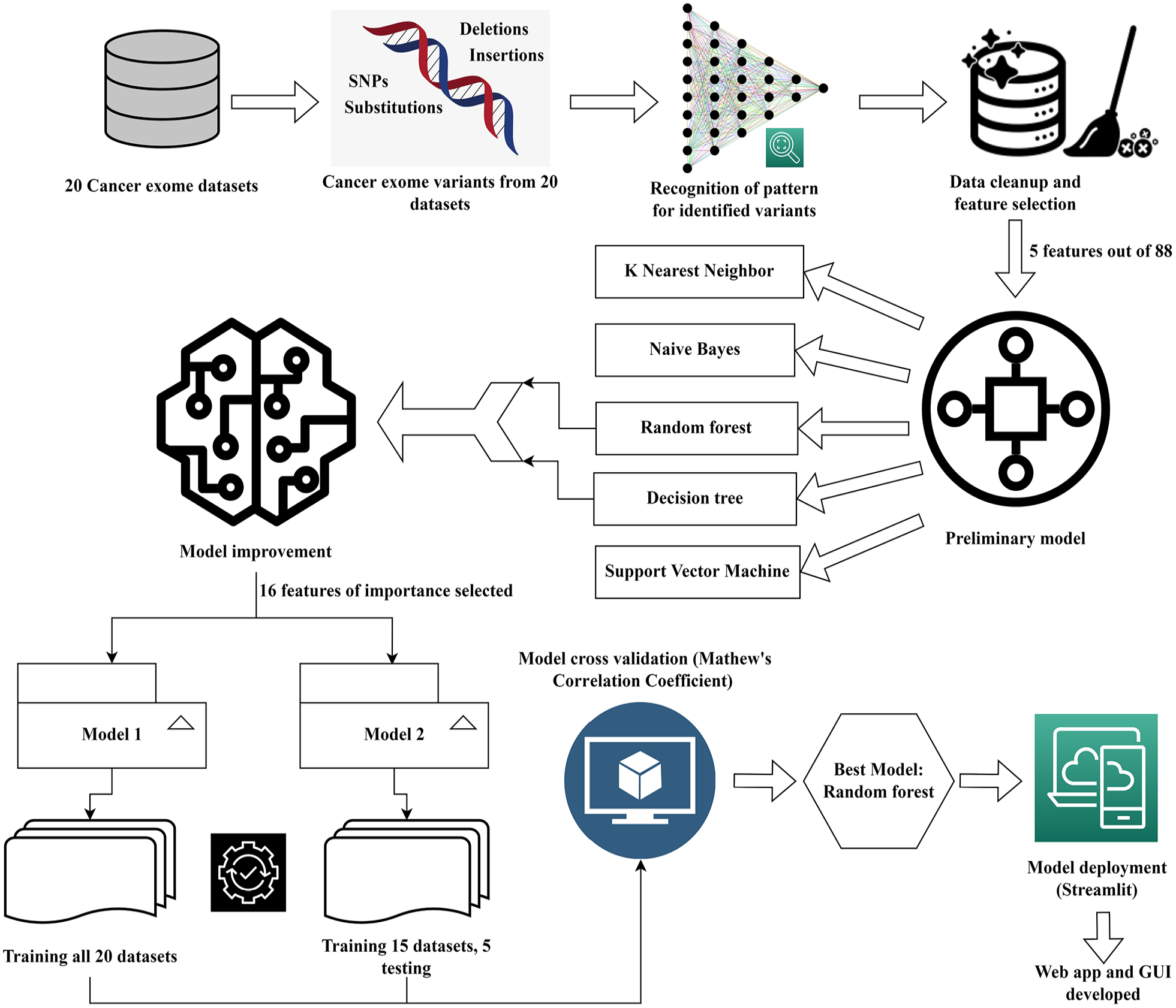
Illustration of the workflow followed for building the decision support system for various cancer types. This figure was drawn using draw.io.

Evaluation parameters

All the models were evaluated based on the following statistical parameters, as given in Gupta and Garg.³⁹

\begin{array}{l} Accuracy = (True positive + True negative) \\ / (\begin{array}{l} True positive + False positive \\ + False negative + True negative \end{array}) \end{array}

Precision = True positive / (True positive + False positive)

Recall = True positive / (True positive + False negative)

F1 - score = 2 * (Precision * Recall) / (Precision + Recall)

\begin{array}{l} Matthe w^{'} s correlation coefficient = \\ \frac{(True positive * True negative) - (False positive * False negative) /}{\sqrt{\begin{array}{l} (True positive + False positive) (True positive + False negative) \\ (True negative + False positive) (True negative + False negative) \end{array}}} \end{array}

Model deployment

To further enhance and allow appropriate use of the designed ML model, it is essential that the model is deployed in a suitable setting. This is primarily done to take complete advantage of the decision support model and the machine learning algorithms used to deploy it in a clinical setting to obtain patient-level predictions. For this purpose, the current DSS model was deployed using Streamlit.⁴⁰ Streamlit is an open-source python library that is used for constructing customized web applications for machine learning algorithms in an uncomplicated manner, that is easy to navigate. All the necessary libraries should be installed after creating a virtual environment. The prediction code is present in a .py file that comprises of a function which takes an image that the user has uploaded and predicts the results by displaying the corresponding probability value. This working principle of Streamlit was utilized in the present study to deploy the designed model.^40,41 The deployed model can be used easily by all users and is accessible via https://share.streamlit.io/sabhapathi0306/streamlit/main/dss.py. The codes employed for deploying the model can be viewed in https://github.com/VN-Lab/DSS.

Results

Pattern recognition for identified variants

A basic pattern was identified and the common single nucleotide polymorphisms (SNPs) across every cancer exome dataset was identified. Nucleotide alteration from C-to-T and G-to-A were found to be most common among all 20 exome datasets. Nucleotide change from G-to-T occurred among 4 cancer exome datasets which all belong to non BRCA1/BRCA2 familial breast cancer. The mutational change from C-to-T occurred in 17 out of 20 exome datasets. Likewise, change from G-to-A occurred in 16 out of 20 exome datasets. Overall, base substitution C-to-T appeared 198 times out of the 4181 variants (raw mutations file-Supplemental File S1) and G-to-A appeared 191 times. In most cases, these 2 nucleotide alterations were found to be frequently occurring. The identification of this common mutational patterns is elucidated in Table 2.

Table 2.

Common mutational patterns recognized for 20 cancer exome datasets for 5 cancer types.

Cancer type	Cancer Exome ID	Most common SNPs and its frequencies of occurrence
Cancer type	Cancer Exome ID	G-A	A-G	C-T	A-T	T-A	G-T	A-C	C-A
Interhepatic cholangiocarcinoma	SRR900123	129	-	127	-	-	-	-	-
	SRR900099	13	-	8	-	-	-	-	-
	SRR894452	-	-	-	61	55	-	-	-
Human Diffuse Type Gastric Cancer	SRR941051	46	-	57	-	-	-	-	-
	SRR941052	37	-	45	-	-	-	-	-
	SRR941053	21	-	28	-	-	-	-	-
	SRR941054	191	-	198	-	-	-	-	-
Non BRCA1/BRCA2 familial breast cancer	ERR166304	-	-	-	-	-	31	39	31
	ERR166307	-	11	11	-	-	14		11
	ERR166310	10	-	13	-	-	-	-	-
	ERR166312	14	-	18	-	-	-	-	-
	ERR166335	8	-	10	-	-	-	-	-
	ERR166336	12	-		-	-	12	-	-
	ERR166303	-	-	14	-	-	11	-	-
Pancreatic adenocarcinoma	ERR232255	35	-	25	-	-	-	-	-
	ERR232254	31	-	29	-	-	-	-	-
	ERR232253	33	-	26	-	-	-	-	-
High-grade serous ovarian cancer	ERR035489	33	-	39	-	-	-	-	-
	ERR035488	36	-	38	-	-	-	-	-
	ERR035487	36	-	36	-	-	-	-	-

Cancer classification model using machine learning algorithms

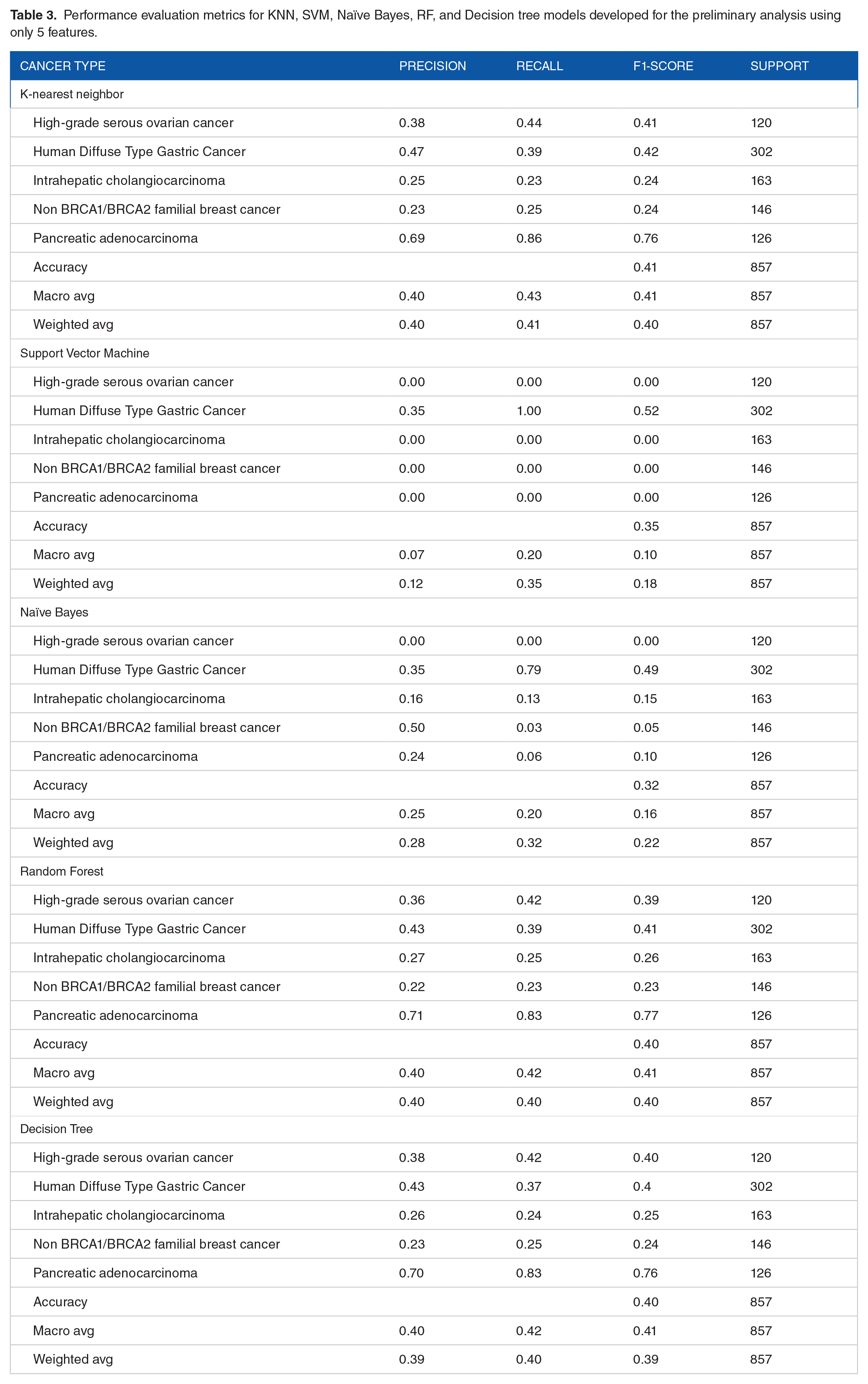
When an initial analysis was carried out with only 5 features, the model did not provide a good prediction due to less correlation between the selected features as observed in the correlation heat map (Figure 2). The heat map showed that correlation between the features was found to be less than .1. Further, from the pairplot, it was noted that the features did not show good correlation with each other (Figure 2). When KNN supervised ML algorithm was used, the weighted average for precision was found to be 0.40, 0.41 for recall and 0.40 for F1-score. The accuracy of the model was found to be 41%. Likewise, the weighted average score for precision was found to be 0.11, 0.34 for recall and 0.17 for F1-score when SVM model was employed. The accuracy of the model was observed to be 34%. With Naïve Bayes, the weighted average was for precision was found to be 0.28, 0.32 for recall and 0.22 for f1-score. The accuracy of the model was observed to be 32%. Likewise, for the decision tree algorithm, the weighted average was found to be 0.39 for precision, 0.40 for recall and 0.39 for f1-score. The model accuracy showed 40%. With RF algorithm, the weighted average was observed to be 0.39 for precision, 0.41 for recall and 0.40 for F1-score. Model accuracy when RF was used was observed to be 41% (Table 3). Thus, although decision tree and RF models showed a higher accuracy, it was still lesser than expected and the output predictions were incorrect due to less training scores. Hence, an improvement in the model was carried out using the afore-mentioned 2 approaches using decision tree and RF.

Figure 2.

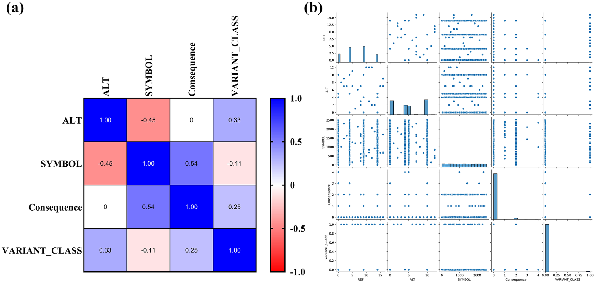
Data visualization for preliminary features selected for model building: (a) correlation heat map for initial model built using 5 ML methods and (b) pairplot of the selected features revealed weak correlation. Since very few features were selected, the correlation between the features were not conclusive.

Table 3.

Performance evaluation metrics for KNN, SVM, Naïve Bayes, RF, and Decision tree models developed for the preliminary analysis using only 5 features.

Cancer type	Precision	Recall	F1-score	Support
K-nearest neighbor
High-grade serous ovarian cancer	0.38	0.44	0.41	120
Human Diffuse Type Gastric Cancer	0.47	0.39	0.42	302
Intrahepatic cholangiocarcinoma	0.25	0.23	0.24	163
Non BRCA1/BRCA2 familial breast cancer	0.23	0.25	0.24	146
Pancreatic adenocarcinoma	0.69	0.86	0.76	126
Accuracy			0.41	857
Macro avg	0.40	0.43	0.41	857
Weighted avg	0.40	0.41	0.40	857
Support Vector Machine
High-grade serous ovarian cancer	0.00	0.00	0.00	120
Human Diffuse Type Gastric Cancer	0.35	1.00	0.52	302
Intrahepatic cholangiocarcinoma	0.00	0.00	0.00	163
Non BRCA1/BRCA2 familial breast cancer	0.00	0.00	0.00	146
Pancreatic adenocarcinoma	0.00	0.00	0.00	126
Accuracy			0.35	857
Macro avg	0.07	0.20	0.10	857
Weighted avg	0.12	0.35	0.18	857
Naïve Bayes
High-grade serous ovarian cancer	0.00	0.00	0.00	120
Human Diffuse Type Gastric Cancer	0.35	0.79	0.49	302
Intrahepatic cholangiocarcinoma	0.16	0.13	0.15	163
Non BRCA1/BRCA2 familial breast cancer	0.50	0.03	0.05	146
Pancreatic adenocarcinoma	0.24	0.06	0.10	126
Accuracy			0.32	857
Macro avg	0.25	0.20	0.16	857
Weighted avg	0.28	0.32	0.22	857
Random Forest
High-grade serous ovarian cancer	0.36	0.42	0.39	120
Human Diffuse Type Gastric Cancer	0.43	0.39	0.41	302
Intrahepatic cholangiocarcinoma	0.27	0.25	0.26	163
Non BRCA1/BRCA2 familial breast cancer	0.22	0.23	0.23	146
Pancreatic adenocarcinoma	0.71	0.83	0.77	126
Accuracy			0.40	857
Macro avg	0.40	0.42	0.41	857
Weighted avg	0.40	0.40	0.40	857
Decision Tree
High-grade serous ovarian cancer	0.38	0.42	0.40	120
Human Diffuse Type Gastric Cancer	0.43	0.37	0.4	302
Intrahepatic cholangiocarcinoma	0.26	0.24	0.25	163
Non BRCA1/BRCA2 familial breast cancer	0.23	0.25	0.24	146
Pancreatic adenocarcinoma	0.70	0.83	0.76	126
Accuracy			0.40	857
Macro avg	0.40	0.42	0.41	857
Weighted avg	0.39	0.40	0.39	857

Improving model accuracy

Since the features selected in the initial attempt did not produce expected outcomes, an attempt to improve the model via the 2 stated methods yielded tremendous outcomes with doubled accuracy.

Method 1: Training all variants from 20 cancer exome datasets

When 16 features were selected and all 20 exome data were trained, the correlation between the features were found to be good, as observed in the correlation heat map (Figure 3). The pairplot for the same also showed good relationship between the features (Figure 4). Despite this, the target classes were imbalanced, hence these were balanced using SMOTE. Initially, human diffuse type gastric cancer had 35.58% of the overall mutation data, 12.41% in high-grade serous ovarian cancer, 14.87% for pancreatic adenocarcinoma, 16.61% for non BRCA1/BRCA2 familial breast cancer and 20.54% in intrahepatic cholangiocarcinoma. After oversampling, the all datasets were balanced equally with 20% variation data in each cancer type (Figure 5). Total training data of the selected features prior to balancing was 2926 and after oversampling via SMOTE, the count of training data increased to 5330 (Table 4).

Figure 3.

Correlation heat map of model improvement approach using 16 important features for building DSS model. The features showed very good correlation among one another. Blue boxes indicate a very high correlation, closer to 1.0, while red boxes point toward a lesser correlation. The results are more conclusive here due to increase in the number of selected features and hence a better DSS model was built.

Figure 4.

Pair plot of the selected features for model improvement. Sixteen substantial features were selected to improve upon the model. The pair plot shows good relationship between each variable in the x-axis to each variable in the y-axis.

Figure 5.

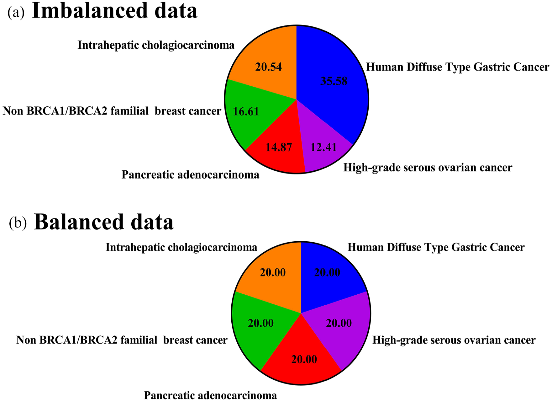
Balancing imbalanced data using SMOTE. (a) Imbalanced classes among the 5 different cancer types before oversampling. Oversampling via SMOTE was employed to balance the classes to obtain more conclusive results. (b) Balanced classes among the 5 cancer types after oversampling.

Table 4.

Total count of training data before and after oversampling using SMOTE.

Count of training data before balancing	2926
Count of training data after balancing	5330

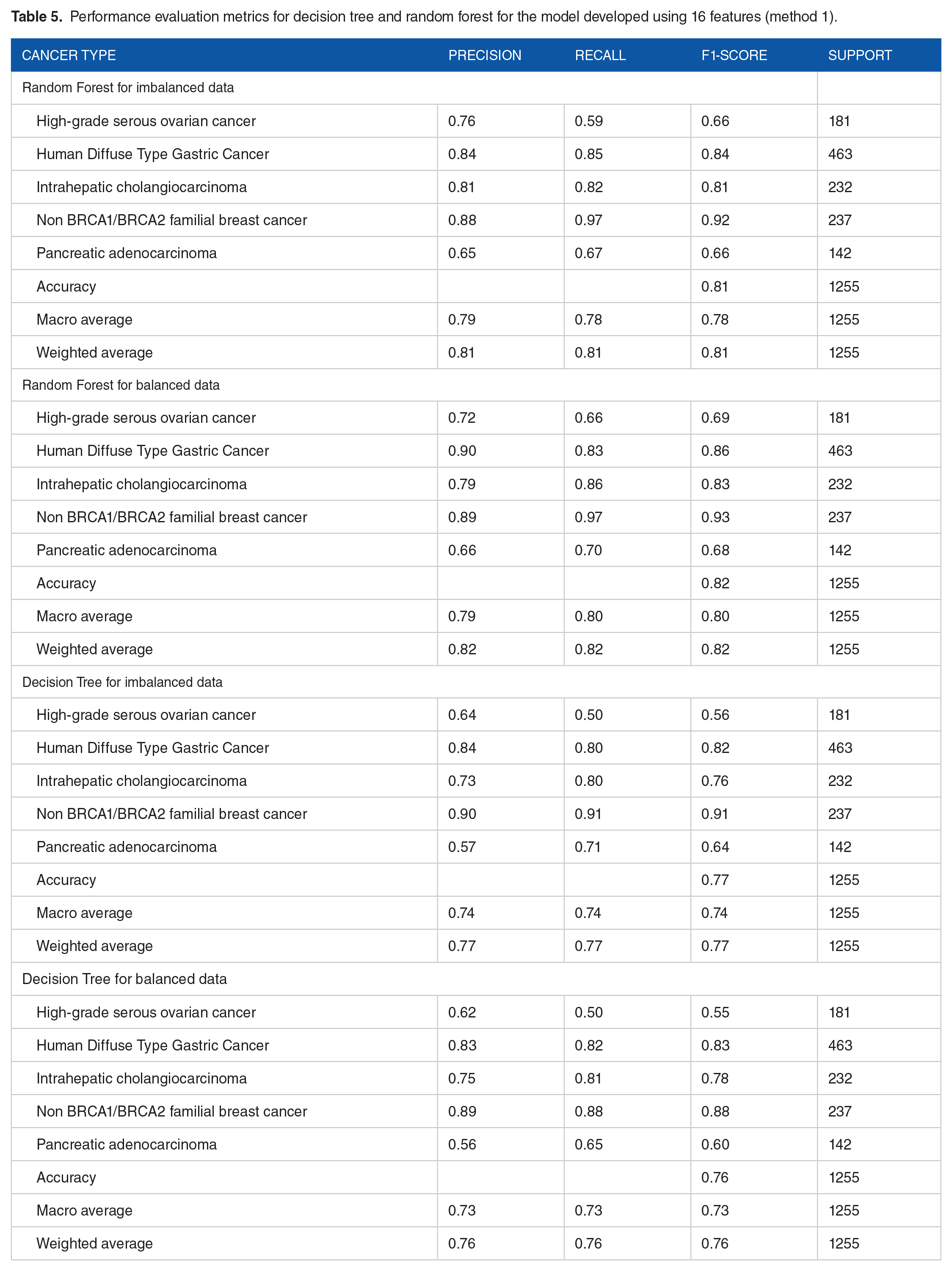
Thus, decision tree model for imbalanced data showed a weighted average value of precision, recall and f1-score of 0.75, bringing the model accuracy up to 75%. When the dataset of each exome sample was balanced, the weighted average for precision, recall and f1-score were found to be 0.77, further improving the model accuracy to 77%. To compare this model with RF, RF for imbalanced data revealed the weighted average values for precision, recall and f1-score to be 0.81, with a model accuracy of 81%. The RF model for balanced data revealed the weighted average for precision was found to be 0.82, 0.82 for recall and 0.82 for f1-score, further upping the accuracy of balanced model to 82% (Table 5).

Table 5.

Performance evaluation metrics for decision tree and random forest for the model developed using 16 features (method 1).

Cancer type	Precision	Recall	F1-score	Support
Random Forest for imbalanced data
High-grade serous ovarian cancer	0.76	0.59	0.66	181
Human Diffuse Type Gastric Cancer	0.84	0.85	0.84	463
Intrahepatic cholangiocarcinoma	0.81	0.82	0.81	232
Non BRCA1/BRCA2 familial breast cancer	0.88	0.97	0.92	237
Pancreatic adenocarcinoma	0.65	0.67	0.66	142
Accuracy			0.81	1255
Macro average	0.79	0.78	0.78	1255
Weighted average	0.81	0.81	0.81	1255
Random Forest for balanced data
High-grade serous ovarian cancer	0.72	0.66	0.69	181
Human Diffuse Type Gastric Cancer	0.90	0.83	0.86	463
Intrahepatic cholangiocarcinoma	0.79	0.86	0.83	232
Non BRCA1/BRCA2 familial breast cancer	0.89	0.97	0.93	237
Pancreatic adenocarcinoma	0.66	0.70	0.68	142
Accuracy			0.82	1255
Macro average	0.79	0.80	0.80	1255
Weighted average	0.82	0.82	0.82	1255
Decision Tree for imbalanced data
High-grade serous ovarian cancer	0.64	0.50	0.56	181
Human Diffuse Type Gastric Cancer	0.84	0.80	0.82	463
Intrahepatic cholangiocarcinoma	0.73	0.80	0.76	232
Non BRCA1/BRCA2 familial breast cancer	0.90	0.91	0.91	237
Pancreatic adenocarcinoma	0.57	0.71	0.64	142
Accuracy			0.77	1255
Macro average	0.74	0.74	0.74	1255
Weighted average	0.77	0.77	0.77	1255
Decision Tree for balanced data
High-grade serous ovarian cancer	0.62	0.50	0.55	181
Human Diffuse Type Gastric Cancer	0.83	0.82	0.83	463
Intrahepatic cholangiocarcinoma	0.75	0.81	0.78	232
Non BRCA1/BRCA2 familial breast cancer	0.89	0.88	0.88	237
Pancreatic adenocarcinoma	0.56	0.65	0.60	142
Accuracy			0.76	1255
Macro average	0.73	0.73	0.73	1255
Weighted average	0.76	0.76	0.76	1255

Since the best model was found to be Random Forest, an ROC curve plotted for both decision tree and random forest models to obtain additional confirmation on random forest’s effectiveness, which revealed area under the curves for the 5 classes of cancers selected for building the model. The area under the curve (AUC) for random forest model was found to be 0.93 for high grade serous ovarian cancer, 1.00 for non BRCA1/BRCA2 familial breast cancer, 0.94 for pancreatic adenocarcinoma, 0.97 for intrahepatic cholangiocarcinoma and 0.96 for human diffuse type gastric cancer. The AUC for decision tree model was found to be 0.74 for high grade serous ovarian cancer, 0.94 for non BRCA1/BRCA2 familial breast cancer, 0.76 for pancreatic adenocarcinoma, 0.85 for intrahepatic cholangiocarcinoma and 0.85 for human diffuse type gastric cancer (Figure 6, Table 6). From this, it is evident that the areas under the curves were better for random forest model than for decision tree, corroborating the previous outcomes and demonstrating that random forest worked better for accurately predicting the 5 cancer types.

Figure 6.

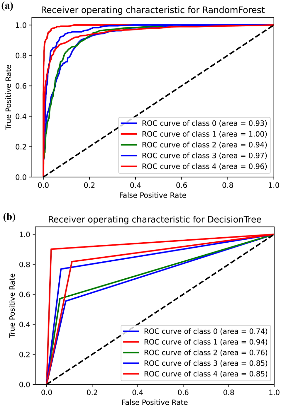
ROC curves for decision tree and random forest models. The x-axis indicated the false positive rate while the y-axis showed the true positive rates. (a) The ROC plot showing area under the curves for random forest model. The AUCs were found to be very close to 1 for all classes, indicating a good model. (b) ROC plot showing area under the curves for decision tree model. The AUCs were found to be lesser than random forest model, proving that random forest worked better for accurately predicting the 5 cancer types.

Table 6.

Area under the curve for the 5 cancer classes used to build the model.

Cancer types	Classes	Area under the curve (AUC)
Random Forest model
High grade serous ovarian cancer	Class 0	0.93
Non BRCA1/BRCA2 familial breast cancer	Class 1	1.00
Pancreatic adenocarcinoma	Class 2	0.94
Intrahepatic cholangiocarcinoma	Class 3	0.97
Human diffuse type gastric cancer	Class 4	0.96
Decision tree model
High grade serous ovarian cancer	Class 0	0.74
Non BRCA1/BRCA2 familial breast cancer	Class 1	0.94
Pancreatic adenocarcinoma	Class 2	0.76
Intrahepatic cholangiocarcinoma	Class 3	0.85
Human diffuse type gastric cancer	Class 4	0.85

Method 2: Training variants from 15 datasets and testing 5 datasets

When 15 exome variation datasets were used for training and 5 for testing, it was observed that the model predicted accurately for only 2 types of cancers- pancreatic adenocarcinoma and non-BRCA1/BRCA2 familial breast cancer, while the prediction was found to be inaccurate for the remaining 3 cancer types. Out of all the cancer types, pancreatic adenocarcinoma showed 97.80% prediction and non BRCA1/BRCA2 familial breast cancer displayed 97.83% prediction.

Model cross-validation using Matthew’s correlation co-efficient

When the model was cross-validated using Matthew’s correlation coefficient for method 1, for imbalanced data, the performance metric values for MCC cross validation was found to be 0.7797 and 0.7881 for MCC test. Likewise, for balanced data, the MCC cross validation value was observed to be 0.9356 and 0.7796 for MCC test. For method 2, the Matthew’s correlation coefficient was found to be 0.9365 (Table 7). Therefore, from this, it is evident that the MCC scores were better for balanced data than imbalanced and the cross validation of the model proved that the designed DSS model is highly accurate.

Table 7.

The Matthew’s correlation co-efficient and MCC test values for method 1 and method 2 to cross-validate the model.

Type of data	MCC_CV	MCC_test
Method 1
Imbalanced data	0.779741	0.788190
Balanced data	0.935611	0.779654
Method 2
Data	0.936585	-

Model deployment

The deployed model, now available as a web application, predicts the model based on already trained model. The model GUI provides the basic steps that the users can follow to upload their files and obtain results. The uploaded files (200 MB limit) must contain the required columns that will be used to predict the cancer type. The NAN processing should then be selected according to the user’s requirement. The user can either drop the values or calculate the mean for the same by choosing the suitable options in the drop-down menu for NAN processing. For reference, a sample data file is provided which the users can go through and make their data in the appropriate format. The files can be dragged and dropped or browsed and uploaded in the side bar provided in the application. One of the 3 calculations can be carried out by selecting the options- data visualization or testing or both. In data visualization, a correlation heat map and a pairplot for the dataset file uploaded is obtained. In the testing option, the data file uploaded will be tested with the trained model and graphical output for the same is revealed. The third selection reveals outcomes of both data visualization and testing. Additionally, the user can select the type of graph that will be displayed as prediction result- a heat map of correlation of the features or a pairplot. The about us page reveals information on the web application and a source code link for the same that connects to the Github repository, is also provided. Screenshots of the GUI of the deployed model, with the options it displays is provided in Figure 7 and a sample dataset run is provided in Figure 8.

Figure 7.

Home page of the decision support system deployed on Streamlit. The web application provides several options such as choosing the file of interest, selecting the NAN process method, data visualization, data testing or performing both. The predictions are provided based on an already trained model.

Figure 8.

Sample results viewed on the web application when the original file was run: (a) shows the original file and the features required for the system to run the operation and (b) sample correlation heat map obtained when the file was run on the system.

Discussion

The current study presents results that have not been previously reported where 5 different cancer types have been used to build a single all-in-one decision support model. Another contribution of our study is toward the use of this model as a base for similar upcoming models, not only for cancer but for other diseases as well. This preliminary research serves to aid in early decision making. Moreover, several variables were considered in the development of the model and web application. These variables, through our methods were proved to be important attributes to the different types of cancers and therefore contributed to better classifications. Decision support systems for personalized radiation oncology have been developed previously for the prediction of normal tissue toxicity and tumor responses.⁴² Additionally, prognostic DSS model has also been built previously using ML and random optimization by the extrication of prognostic data for breast cancers.⁴³ Classification using computed tomography scan images have also been carried out using deep fully convoluted neural networks to improve detection of pulmonary cancers.⁴⁴ Studies have also highlighted the importance of machine learning and DSS in healthcare for the identification of complicated disease patterns, detection and diagnosis of diseases, and suggestion of appropriate treatment strategies.⁴⁵ The present study worked on similar concepts with the added value additions as stated above. Thus, the following sections discuss the results obtained in the present study with similar such work to highlight the importance of the present research.

Previous studies have stated distinctly the significance of employing pattern recognition for the detection of various types of cancers and discusses that to predict the occurrence of cancer in a better way, different integrative patterns that arise from analysis of omics data such as genomics, proteomics, transcriptomics, and metabolomics vastly contribute to cancer precision medicine.⁴⁶ The current study has also recognized patterns from SNP data that were previously collected using omics approaches in our previous study.¹⁶ Moreover, another study has identified intelligent phenotypic patterns using computer-aided detection of genetic syndromes.⁴⁷ To add to this list, lung cancer has been previously diagnosed using patterns that were identified using deep learning.⁴⁸ In the present research, the basic recognized patterns assist in rapid cancer type detection that can be integrated in analogous decision support models. Generally, repetitive base substitutions from G-to-A have been previously identified in the cancer of the gall bladder⁴⁹ and high rates of C-to-T alterations have been reported in several metastatic melanomas.⁵⁰ Hence, the current work has reported beneficial patterns, which when further analyzed will aid in early cancer diagnosis.

When an initial analysis was carried out with only 5 features, the model did not provide a good prediction due to less correlation between the selected features as observed in the correlation heat map (Figure 3). Although DT and RF models showed a higher accuracy, it was still lesser than expected and the output predictions were incorrect due to less training scores. Hence, an improvement in the model was carried out using the afore-mentioned 2 approaches using decision tree and RF. A recent study has reported using machine learning models such as KNN, naïve bayes, SVM, decision tree and logistic regression for early breast cancer detection, wherein, the study concluded that aside from KNN algorithm, logistic regression, decision tree and naïve bayes showed good performance, with SVM having the best accuracy and performance.⁵¹ Likewise, another study tested out several ML algorithms such as KNN, SVM, RF, Naïve Bayes, decision tree and logistic regression for breast cancer prediction and reported SVM to be the best performer.⁵² In the present work however, random forest model and decision tree performed better in terms of preliminary model accuracy, which were then taken forward for model improvement studies.

Additionally, when the initial models were designed using 5 ML algorithms, it was observed that selecting different and a greater number of features increased the model accuracy, suggesting that features play a very important role in model building. By designing ML based DSS with appropriate features, accuracy of the best model shot up to 82%, thereby, acting as a powerful tool to doctors and patients. Increasing the size of the data further may aid in providing more variability to the data, however, at the cost of increasing the classification errors. From AUC, it was evident that curves were better for RF than for DT model, corroborating the previous outcomes and demonstrating that random forest worked better for accurately predicting the 5 cancer types. Furthermore, among all cancer types, pancreatic adenocarcinoma showed 97.80% prediction and non BRCA1/BRCA2 familial breast cancer displayed 97.83% prediction. This indicated that although the model has high accuracy of 82%, when datasets were split for training and testing, some issues persisted. This could be associated with lesser number of datasets and reduced variability and thus, the problem will be resolved by adding more mutations from different cancer exome datasets to enhance the variability and bring about accurate predictions, as part of the prospective work. Another important way of improving the number of data available would be to use Generative Adversarial Networks (GAN) that could add to better predictability, as part of future work.

A recent study has used ML models to predict the survival prognosis of breast cancer patients, wherein, the training datasets were split into 5 subsets for testing.⁵³ Similarly, in the present study, the approach used in method 2 was to test 5 datasets and train 15, so as to assess the model ability when new samples were given as input. Additionally, previous studies have also effectively predicted the metastasis of breast cancers using serum biomarkers such as CEA, CA15-3, and sHER2 via machine learning models. The study determined random forest to be the optimum model for predicting metastasis 3 months in advance.⁵⁴ Likewise, another study utilized ensemble machine learning techniques, specifically, an ensemble of random forests to predict abnormalities related to cervical cancer.⁵⁵ The present study also reports random forest as an optimal machine learning algorithm for designing a DSS model with a high accuracy. Typically, DSS models are built for specific cancer types, as evidenced from previous studies. However, our study has explored all possible variations from 20 cancer exomes, belonging to 5 different cancer types, thereby offering a wide range of accurate predictions for early diagnosis of various cancers and better treatment management, making it a novel finding.

The MCC correlation proved that our model showed very good accuracy and corroborated the results obtained in previous steps. A study carried out previously to predict the immune responsiveness against specific cancer types reported an 88% accuracy using SVM model and MCC value of 0.27.⁵⁶ The current study demonstrated a high MCC value of 0.93, that cross validated the accuracy obtained in our model from both the approaches. Moreover, research has stated that an MCC value close to +1 indicates very good performance, while closer to −1 suggests bad model performance.⁵⁷ Since the current study showed very good MCC values for both method 1 and method 2, it indicates that the model developed is robust.

Additionally, other similar studies to our work have been carried out previously and web applications have been developed. Comparisons for the same is provided here to showcase the novelty of our work. A recent study created a decision support system for predicting the probability of 30-day mortality of post-operative specific spinal metastasis.⁵⁸ This model used 4 machine learning techniques and deployed the designed model as an open access web page via Shiny, a publicly available software interface. Another study has designed an online calculator for the survival prediction of patients suffering from glioblastoma, using machine learning algorithms such as regression.⁵⁹ The study utilized Shiny to deploy the model, which can now be accessible by all. In the current study, Streamlit was employed for deploying the designed model to make it accessible for all users. With the right information, user can upload the files and obtain required results and plots. Since Python was employed as the main language for implementing the model, Streamlit was used, contrary to the above-mentioned studies where R was used for analytics, hence deployed using Shiny. The present study is an extension and part of our previous work, wherein, the preliminary DSS model building was carried out.^60,61

Conclusion and Future Scope

Since currently, there is a paucity in precise cancer diagnosis, a need for appropriate prediction models that aid diagnosticians/researchers/clinicians to make that decision is required. The present study designed a model-driven decision support system using supervised machine learning algorithms. An initial attempt using classifiers such as K-nearest neighbor, support vector machine, decision tree, naïve bayes and random forest revealed that random forest and decision are potentially accurate models. When all 20 datasets were trained after efficiently balancing the datasets, random forest model provided a high accuracy of 82% with correct predictions for all 5 cancer types. However, when 5 datasets were tested and 15 trained, predictions were accurate for only pancreatic adenocarcinoma and non BRCA1/BRCA2 familial breast cancers. A cross-validation of the model via Matthew’s correlation coefficient proved that our model is highly precise and is designed accurately. This model was successfully deployed as a web-application that is easy to navigate so that it can have a better reach. In the future, the authors have planned to extend the study by adding more variation data and datasets to improve the model accuracy and to include other cancer types. By implementing advanced ML techniques such as ensemble algorithms and XgBoost, the current model can further be enhanced. Thus, the present study provides massive insights into the use of the designed model for easy diagnosis of various cancer types.

Supplemental Material

sj-csv-1-cix-10.1177_11769351221147244 – Supplemental material for Decision Support System and Web-Application Using Supervised Machine Learning Algorithms for Easy Cancer Classifications

Supplemental material, sj-csv-1-cix-10.1177_11769351221147244 for Decision Support System and Web-Application Using Supervised Machine Learning Algorithms for Easy Cancer Classifications by K Chandrashekar, Anagha S Setlur, Adithya Sabhapathi C, Satyam Suresh Raiker, Satyam Singh and Vidya Niranjan in Cancer Informatics

Supplemental Material

sj-xlsx-2-cix-10.1177_11769351221147244 – Supplemental material for Decision Support System and Web-Application Using Supervised Machine Learning Algorithms for Easy Cancer Classifications

Supplemental material, sj-xlsx-2-cix-10.1177_11769351221147244 for Decision Support System and Web-Application Using Supervised Machine Learning Algorithms for Easy Cancer Classifications by K Chandrashekar, Anagha S Setlur, Adithya Sabhapathi C, Satyam Suresh Raiker, Satyam Singh and Vidya Niranjan in Cancer Informatics

Supplemental Material

sj-xlsx-3-cix-10.1177_11769351221147244 – Supplemental material for Decision Support System and Web-Application Using Supervised Machine Learning Algorithms for Easy Cancer Classifications

Supplemental material, sj-xlsx-3-cix-10.1177_11769351221147244 for Decision Support System and Web-Application Using Supervised Machine Learning Algorithms for Easy Cancer Classifications by K Chandrashekar, Anagha S Setlur, Adithya Sabhapathi C, Satyam Suresh Raiker, Satyam Singh and Vidya Niranjan in Cancer Informatics

Footnotes

Acknowledgements

We would like to thank Dr. Shobha G, Professor, Department of Computer Science and Engineering, RV College of Engineering, Bangalore, for providing us with QuADro GV100 GPU for performing computational analysis. The authors would like to acknowledge Mr. Akshay Uttarkar for reviewing the manuscript and providing valuable suggestions. We would also like to acknowledge Ms. Padmavathi P for providing insights on the methodology. Special thanks to Mr. Aravind Ganessin, Managing Director, Intergene Biosciences Pvt. Ltd, Bangalore, for the inputs.

Funding:

The author(s) received no financial support for the research, authorship, and/or publication of this article.

Declaration Of Conflicting Interests:

The author(s) declared no potential conflicts of interest with respect to the research, authorship, and/or publication of this article.

Author Contributions

Chandrashekar K (C.K) and Anagha S Setlur (A.S.S): collected the preliminary data required for the study, analyzed the data and wrote the main manuscript.

Adithya Sabhapathi C (A.S.C), Satyam Suresh Raiker (S.S.R) and Satyam Singh (S.S): Implemented the algorithms required for the study and analyzed the data.

Vidya Niranjan (V.N): Conceptualized the idea, analyzed the results and project implementation. All authors reviewed the manuscript.

Data Availability

The derivative datasets used in the current study are generated from analysis of datasets downloaded from publicly available NCBI SRA database. The below NCBI SRA datasets were used in our previous work to arrive at the data that was used in the current study.

SRR894452, SRR900123, SRR900099, SRR941051, SRR941052, SRR941053, SRR941054, ERR166303, ERR166304, ERR166307, ERR166310, ERR166312, ERR166335, ERR166336, ERR035487, ERR035488, ERR035489, ERR232253, ERR232254, ERR232255

The raw data of identified variations used for building the DSS system in the current study are available in Supplemental File S1. For further reference, clinical information on the datasets used, as obtained from NCBI-SRA are provided as Supplemental File S2. Supplemental File S3 shows the initial pre-processing and feature selection based on NaN value criterion and the ANOVA test score and P values for the initial selected 19 features.

Supplemental Material

Supplemental material for this article is available online.

References

Liu Sheng

. Decision support for healthcare in a new information age. Decis Support Syst. 2000;30:101-103.

Hicks

Dunnenberger

Gumpper

Haidar

Hoffman

JM.

Integrating pharmacogenomics into electronic health records with clinical decision support. Am J Health Syst Pharm. 2016;73:1967-1976.

Pagel

Kim

Moad

, et al. Integrated informatics analysis of cancer-related variants. JCO Clin Cancer Informat. 2020;4:310-317.

Irmisch

The tumor profiler study: integrated, multi-omic, functional tumor profiling for clinical decision support. Cancer Cell. 2021;39:288-293.

Yalcin

Danisik

Baygin

Acar

Systems biology and experimental model systems of Cancer. J Pers Med. 2020;10:180.

West

Mangiameli

Rampal

West

Ensemble strategies for a medical diagnostic decision support system: A breast cancer diagnosis application. Eur J Oper Res. 2005;162:532-551.

Pawloski

Brooks

Nielsen

Olson-Bullis

BA.

A systematic review of clinical decision support systems for clinical oncology practice. J Natl Compr Canc Netw. 2019;17:331-338.

Ash

McCormack

Sittig

Wright

McMullen

Bates

DW.

Standard practices for computerized clinical decision support in community hospitals: a national survey. J Am Med Inform Assoc. 2012;19:980-987.

Moreira

MWL

Rodrigues

JJPC

Korotaev

Al-Muhtadi

Kumar

. A comprehensive review on smart decision support systems for health care. IEEE Syst J. 2019;13:3536-3545.

10.

Holsapple

. DSS Architecture and Types. In Handbook on Decision Support Systems. Springer; 2008: 163-189.

11.

Ramamurthy

King

Premkumar

User characteristics—DSS effectiveness linkage: an empirical assessment. Int J Man Mach Stud. 1992;36:469-505.

12.

Alshibly

HH.

Investigating decision support system (DSS) success: a partial least squares structural equation modeling approach. J Bus Stud Q 2015;6:56.

13.

Safdar

Zafar

Khan

NF.

Machine learning based decision support systems (DSS) for heart disease diagnosis: a review. Artif Intell Rev. 2018;50:597-623.

14.

Mohammed

Abd Ghani

Arunkumar

, et al. Retracted article: decision support system for nasopharyngeal carcinoma discrimination from endoscopic images using artificial neural network. J Supercomput. 2020;76:1086-1104.

15.

Puppala

Ezeana

, et al. A deep learning–based decision support tool for precision risk assessment of breast cancer. JCO Clin Cancer Informat. 2019; 3:1-12.

16.

Padmavathi

Setlur

Chandrashekar

Niranjan

A comprehensive in-silico computational analysis of twenty cancer exome datasets and identification of associated somatic variants reveals potential molecular markers for detection of varied cancer types. Inform Med Unlocked. 2021;26:100762.

17.

Padmavathi

Chandrashekar

Setlur

Niranjan

MutaXome: a novel database for identified somatic variations of in silico analyzed cancer exome datasets. Cancer Inform. 2022;21:11769351221097593.

18.

Pedregosa

Scikit-learn: machine learning in python. J Mach Learn Res. 2011;12:2825-2830.

19.

Ahmad

Quegan

Comparative analysis of supervised and unsupervised classification on multispectral data. Appl Math Sci. 2013;7:3681-3694.

20.

Rashidi

Tran

Betts

Howell

Green

Artificial intelligence and machine learning in pathology: the present landscape of supervised methods. Acad Pathol. 2019;6:2374289519873088.

21.

Singh

Thakur

Sharma

. A review of supervised machine learning algorithms. Paper presented at: 2016 3rd International Conference on Computing for Sustainable Global Development (INDIACom); 2016:1310-1315.

22.

Berrar

Bayes’ theorem and naive Bayes classifier. Encycl Bioinforma Comput Biol; 2018;1:403-412.

23.

John

Langley

Estimating Continuous Distributions in Bayesian Classifiers. Paper presented at: Proceedings of the Eleventh Conference on Uncertainty in Artificial Intelligence; 1995.

24.

Rish

An empirical study of the naive Bayes classifier. IJCAI 2001 workshop on empirical methods in artificial intelligence. 2001;3:41-46.

25.

Hand

Idiot’s Bayes? Not so stupid after all?

Int Stat Rev. 2001;69:385-398.

26.

Nigsch

Bender

van Buuren

Tissen

Nigsch

Mitchell

JB.

Melting point prediction employing k-nearest neighbor algorithms and genetic parameter optimization. J Chem Inf Model. 2006;46:2412-2422.

27.

Tran

Sen

Palmieri

, et al. Artificial intelligence and machine learning for predicting acute kidney injury in severely burned patients: a proof of concept. Burns. 2019;45:1350-1358.

28.

Gholami

Fakhari

. Support vector machine: principles, parameters, and applications. In: Samui P, Sekhar S, Balas VE, eds. Handbook of Neural Computation. Academic Press, Elsevier; 2017: 515-535.

29.

Suresh

Udendhran

Balamurgan

Hybridized neural network and decision tree based classifier for prognostic decision making in breast cancers. Soft Comput. 2020;24:7947-7953.

30.

Liaw

Wiener

Classification and regression by randomForest. R News. 2002;2:18-22.

31.

Javeed

Zhou

Yongjian

Qasim

Noor

Nour

An intelligent learning system based on random search algorithm and optimized random forest model for improved heart disease detection. IEEE Access. 2019;7:180235-180243.

32.

Cox

PAIRPLOT: Stata module for plots of paired observations; 2007.

33.

Kendig

Baheti

Bockol

, et al. Sentieon DNASeq variant calling workflow demonstrates strong computational performance and accuracy. Front Genet. 2019;10:736.

34.

Chawla

Bowyer

Hall

Kegelmeyer

WP.

SMOTE: synthetic minority over-sampling technique. J Artif Intell Res. 2002;16:321-357.

35.

Fernandez

Garcia

Herrera

Chawla

NV.

SMOTE for learning from imbalanced data: progress and challenges, marking the 15-year anniversary. J Artif Intell Res. 2018;61:863-905.

36.

Skryjomski

Krawczyk

Influence of minority class instance types on SMOTE imbalanced data oversampling. Paper presented at: First international workshop on learning with imbalanced domains: theory and applications: 2017; 7-21.

37.

Chicco

Jurman

The advantages of the Matthews correlation coefficient (MCC) over F1 score and accuracy in binary classification evaluation. BMC Genomics. 2020;21:6.

38.

Zhu

On the performance of Matthews correlation coefficient (MCC) for imbalanced dataset. Pattern Recognit Lett. 2020;136:71-80.

39.

Gupta

Garg

Breast cancer prediction using varying parameters of machine learning models. Procedia Comput Sci. 2020;171:593-601.

40.

Singh

. Deploy Machine Learning Models to Production. Springer;2021.

41.

Singh

. Machine learning deployment as a web service. In: Deploy Machine Learning Models to Production. Springer; 2021:67-90.

42.

Lambin

Decision support systems for personalized and participative radiation oncology. Adv Drug Deliv Rev. 2017;109:131-153.

43.

Ferroni

Zanzotto

Riondino

Scarpato

Guadagni

Roselli

Breast cancer prognosis using a machine learning approach. Cancers. 2019;11:328.

44.

Masood

Sheng

, et al. Computer-assisted decision support system in pulmonary cancer detection and stage classification on CT images. J Biomed Inform. 2018;79:117-128.

45.

Shailaja

Seetharamulu

Jabbar

MA.

Machine Learning in Healthcare: A Review. Paper presented at: 2018 Second International Conference on Electronics, Communication and Aerospace Technology (ICECA); 2018. doi:10.1109/iceca.2018.8474918.

46.

Cheng

Zhan

Pattern recognition for predictive, preventive, and personalized medicine in cancer. EPMA J. 2017;8:51-60.

47.

Gurovich

Hanani

Bar

, et al. Identifying facial phenotypes of genetic disorders using deep learning. Nat Med. 2019;25:60-64.

48.

Sun

Zheng

Qian

Computer aided lung cancer diagnosis with deep learning algorithms. Medical Imaging 2016: Computer-Aided Diagnosis. vol. 9785; 2016: 97850Z.

49.

Zhang

, et al. Whole-exome and targeted gene sequencing of gallbladder carcinoma identifies recurrent mutations in the ErbB pathway. Nat Genet. 2014;46:872-876.

50.

Wong

Behren

Mar

, et al. Whole exome sequencing identifies a recurrent RQCD1 P131L mutation in cutaneous melanoma. Oncotarget. 2015;6:1115-1127.

51.

Lomboy

KEMR

Hernandez

RM.

A comparative performance of breast cancer classification using hyper-parameterized machine learning models. Int J Adv Technol Eng Explor. 2021;8:1080-1101.

52.

Shamrat

FMJM

Raihan

Rahman

AKMS

Mahmud

Akter

. An analysis on breast disease prediction using machine learning approaches. Int J Sci Technol Res. 2020;9:2450-2455.

53.

Mihaylov

Nisheva

Vassilev

Application of machine learning models for survival prognosis in breast cancer studies. Information. 2019;10:93.

54.

Tseng

Y-J

Huang

Wen

, et al. Predicting breast cancer metastasis by using serum biomarkers and clinicopathological data with machine learning technologies. Int J Med Inform. 2019;128:79-86.

55.

Bountris

Haritou

Pouliakis

Karakitsos

Koutsouris

. A decision support system based on an ensemble of random forests for improving the management of women with abnormal findings at cervical cancer screening. Paper presented at: 37th Annual International Conference of the IEEE Engineering in Medicine and Biology Society (EMBC); 2015:8151-8156.

56.

Polano

Chierici

Dal Bo

, et al. A pan-cancer approach to predict responsiveness to immune checkpoint inhibitors by machine learning. Cancers. 2019;11:1562.

57.

Islam

Haque

Iqbal

Hasan

Kabir

MN.

Breast cancer prediction: a comparative study using machine learning techniques. SN Comput Sci. 2020;1:1-14.

58.

Karhade

Thio

QCBS

Ogink

, et al. Development of machine learning algorithms for prediction of 30-day mortality after surgery for spinal metastasis. Neurosurg. 2019;85:E83-E91.

59.

Senders

Staples

Mehrtash

, et al. An online calculator for the prediction of survival in glioblastoma patients using classical statistics and machine learning. Neurosurg. 2020;86:E184-E192.

60.

Padmavathi

Anagha

Adithya

, et al. Prototype of Decision Support System using Pattern Recognition as an Application of Artificial Intelligence and Machine Learning for Early Diagnosis of Genetic Diseases. Paper presented at: 1244th International Conference on Medical, Biological and Pharmaceutical Sciences (Accepted); 2022. doi:IASTEM.08122021.14897

61.

Pasha Syed

Anbalagan

Setlur

, et al. Implementation of ensemble machine learning algorithms on exome datasets for predicting early diagnosis of cancers. BMC Bioinform. 2022;23:1-24.

Supplementary Material

Please find the following supplemental material available below.

For Open Access articles published under a Creative Commons License, all supplemental material carries the same license as the article it is associated with.

For non-Open Access articles published, all supplemental material carries a non-exclusive license, and permission requests for re-use of supplemental material or any part of supplemental material shall be sent directly to the copyright owner as specified in the copyright notice associated with the article.

0.00 MB

4.66 MB

0.01 MB