Sage Journals: Discover world-class research

Abstract

Prostate cancer is the most frequently diagnosed cancer in men in the United States. The current main methods for diagnosing prostate cancer include prostate-specific antigen test and transrectal biopsy. Prostate-specific antigen screening has been criticized for overdiagnosis and unnecessary treatment, and transrectal biopsy is an invasive procedure with low sensitivity for diagnosis. We provided a quantitative tool using supervised learning with multiparametric imaging to be able to accurately detect cancer foci and its aggressiveness. A total of 223 specimens from patients who received magnetic resonance imaging (MRI) and magnetic resonance spectroscopy imaging prior to the surgery were studied. Multiparametric imaging included extracting T2-map, apparent diffusion coefficient (ADC) using diffusion-weighted MRI, $K^{t r a n s}$ using dynamic contrast-enhanced MRI, and 3-dimensional-MR spectroscopy. A pathologist reviewed all 223 specimens and marked cancerous regions on each and graded them with Gleason scores, which served as the ground truth to validate our prediction model. In cancer aggressiveness prediction, the average area under the receiver operating characteristic curve (AUC) value was 0.73 with 95% confidence interval (0.72-0.74) and the average sensitivity and specificity were 0.72 (0.71-0.73) and 0.73 (0.71-0.75), respectively. For the cancer detection model, the average AUC value was 0.68 (0.66-0.70) and the average sensitivity and specificity were 0.73 (0.70-0.77) and 0.62 (0.60-0.68), respectively. Our method included capability to handle class imbalance using adaptive boosting with random undersampling. In addition, our method was noninvasive and allowed for nonsubjective disease characterization, which provided physician information to make personalized treatment decision.

Keywords

prostate cancer diagnostic imaging multiparametric MRI/MRSI predictive modeling

Background

Prostate cancer is the most frequently diagnosed cancer in men. The American Cancer Society estimated approximately 161 360 new cases of prostate cancer and about 26 730 deaths from prostate cancer in the United States in 2017.¹ Currently, the 2 main methods for diagnosing prostate cancer are prostate-specific antigen (PSA) test in conjunction with a digital rectal examination and transrectal biopsy. Prostate-specific antigen, which is measured by an immunoassay, has gained wide acceptance and approved by Food and Drug Administration as a serum tumor diagnostic marker in the management of prostate cancer.² However, recent studies have shown that some men with low PSA levels (<4.0 ng/mL) have prostate cancer and many men with high PSA levels do not have prostate cancer.³ In addition, it has been shown that there is little to no reduction in prostate cancer–specific mortality resulting from PSA screening, and PSA screening may be responsible for overdiagnosis and unnecessary treatment.⁴ The conflicting evidence on the benefit of PSA makes it an unreliable method for prostate cancer diagnosis.^5,6 The other commonly used diagnostic method, transrectal ultrasound (TRUS)-guided biopsy, uses a 12-core sampling of the prostate gland. It can result in cancers being missed if regions were not sampled.⁷ Even when the biopsy does detect cancer, the localization of tumor within the gland remains imprecise.⁸ Due to the imprecise nature and low sensitivity of the biopsy procedure, patients may need to undergo repeated biopsies or convert to MRI/US fusion or even other types of biopsies.⁹ This may lead to either a delayed detection of aggressive cancer or unnecessary recurrent invasive biopsies in the absence of conclusive results.¹⁰

Recently, multiparametric magnetic resonance (MR) imaging, which combines various functional MRI techniques with conventional T2-weighted imaging, has been established as a method for detection of prostate cancer.^11,12 The functional imaging techniques include diffusion-weighted imaging (DWI), dynamic contrast-enhanced MRI (DCE-MRI) and magnetic resonance spectroscopy imaging (MRSI). Apparent diffusion coefficient (ADC) values from DWI have been used to differentiate prostate tumors from normal tissue as the magnitude of diffusion of the prostate tumors is lower than the normal gland.¹³ Several studies have shown that ADC values are associated with patients’ Gleason scores (GSs).^14–16 The DCE-MRI has also been used to differentiate malignant from normal tissues for the prostate gland.¹⁷ And, MRSI aims to detect alterations in cellular metabolism that occur in prostate cancer.¹⁸

It is known that using conventional T2-weighted imaging alone cannot identify the tumors within the prostate accurately.¹⁹ To overcome this, DCE-MRI was combined with DWI to differentiate central gland cancer from benign prostatic hyperplasia.²⁰ The DWI, DCE-MRI, and MRSI were incorporated to predict prostate cancer aggressiveness.²¹ One group combined T2-weighted imaging, DWI, DCE-MRI,²² and another group combined T2-weighted MRI and ADC MRI²³ for prostate cancer detection.

Although combining several data sources can improve the quality of prediction, extracting complex relationship from multiple sources can be challenging. Advanced predictive models are required in addition to quality imaging sources. Machine learning methods, such as logistic regression, have been proposed to identify prostate cancer.²⁴ However, the challenge is class imbalance, namely, the number of instances of one class (eg, indolent disease samples) far exceeds the other class (eg, highly aggressive cancer samples). If a classifier is created without considering class imbalance, the result could be biased toward the majority class. Several methods have been proposed to deal with class imbalance problem.²⁵ These methods can be categorized into 2 groups: cost sampling methods and data-level approaches.²⁶ The cost sampling methods use an asymmetric cost function to artificially balance the training process.²⁷ However, the data-level approaches turn the imbalanced problem into a balanced one by either oversampling the minority class (replicating minority class observations or creating synthetic data)^28,29 or undersampling (removing observations from the majority class).^30,31

For the cost sampling approaches, the performance of the model heavily relies on the cost parameters and the parameters are not known a priori. And if the correlation between the predictor and output variable is weak, which we have identified is the case for the multiparametric MRI/MRSI data and the GS, using oversampling has a negative effect on the predictive model. Hence, in this study, we used an undersampling approach to systematically deal with class imbalance and developed a noninvasive tool using multiparametric imaging data in supervised machine learning methods.

Methods

Patient cohort and specimen octants generation

Data were collected from 11 patients who had TRUS-guided biopsy-proven prostate cancer and elected to have radical prostatectomy received MRI/MRSI prior to their surgical procedure. The average PSA level of these patients was 9.4 (0.5-29.0) ng/mL. After radical prostatectomy, each prostate specimen was fixed in formalin and high-resolution MR images were obtained prior to whole mount sectioning of the prostate. Axial sections (3 mm) from the specimen were made using an in-house prostate slicer. Hematoxylin-eosin (H&E) staining was performed on 50-µm sections from each of the slides. Digital images of both the slice specimens and the pathologic slides were obtained, which were used to match to the MR images. After discarding unusable slices, the remaining 28 slices were subdivided into octants. This resulted in 223 octants (1 octant was not usable). A GS was given to each of the octant by a pathologist. In our data set, GSs range from 0 to 8, with 0 indicating no cancer cell identified, GS ⩽ 6 indicating indolent (slow-growing or nonaggressive), and GS > 6 indicating aggressive cancer. In Figure 1, we show the distribution of GS in our data set.

Figure 1.

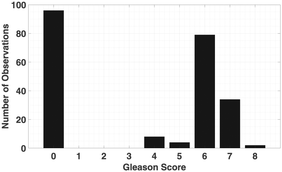
Gleason score histogram.

Multiparametric MRI/MRSI

The following images were acquired: (a) conventional T2-weighted (T2W) images, (b) DWI-MRI, (c) DCE-MRI, and (d) MRSI covering the entire prostate using PRESS localization to attain MR spectroscopy score. Sample images are shown in Figure 2. This particular subject shows a tumor in the peripheral zone (arrows), and while it is difficult to locate the tumor foci on the T2W images and the T2-map, it can be readily detected using ADC and $K^{t r a n s}$ as areas of reduced ADC and elevated $K^{t r a n s}$ , respectively. Spectroscopy data from a selected voxel in the same region show elevated level of choline as compared with the normal tissue and a reduction in the citrate peak. This is the characteristic signature of higher-grade malignancy in the prostate. The location of the tumor with a GS of 7 is confirmed for this patient by histopathology using the H&E stain.

Figure 2.

An example of multiparametric imaging of prostate: Top row: T2-weighted (T2W) image, T2-map, H&E stain (histology). Bottom row: ADC map (DWI), $K^{t r a n s}$ (DCE-MRI), MR spectroscopy. Histology and MR images showing cancer as marked by the arrow, and corresponding spectra from the tumor showing low citrate and high choline. ADC indicates apparent diffusion coefficient; DCE-MRI, dynamic contrast-enhanced magnetic resonance imaging; DWI, diffusion-weighted imaging.

From these images, we extracted 4 types of quantitative features for predictive modeling. From T2W, we use the average of $T_{2}$ values that measures the proton spin decay rate. From DWI-MRI, we extracted the ADC, which measures the magnitude of diffusion. From DCE-MRI, we obtained the volume transfer constant that was extracted using the Tofts kinetic model.³² From MRSI, MR spectroscopy was extracted which is used to estimate the relative concentrations of biochemical compounds in the target area. The distributions of the 4 features were collected using percentiles (eg, 5th, 10th, 50th, 90th, and 95th percentiles). Then, the average and standard deviation of the values for the voxels within each percentile were calculated as input features for our next step predictive modeling. As an illustration, Figure 3 shows the correlation plot for the average of the 50th percentile features with the GS.

Figure 3.

Correlation plot of the average values of the 50th percentile voxels for features (ADC, $K^{t r a n s}$ , spectroscopy score, and T2) and the Gleason scores. ADC indicates apparent diffusion coefficient.

Predictive modeling via supervised machine learning

We considered 2 binary classification problems. In the first one, we aim to distinguish aggressive prostate cancer (GS > 6) from indolent disease and absence of cancer (GS ⩽ 6). In the second classification problem, we aim to detect cancerous samples (GS > 0).

Before building a predictive model, it is critical to handle the class imbalance problem. As seen in Figure 1, the number of nonaggressive cancer samples was 187 and the number of aggressive ones was 36. The ratio was approximately 5:1. When there is an imbalanced distribution in the data set, a typical classifier would be biased toward one class because it has the goal of maximizing overall accuracy. Because there was a weak correlation between the features and the GS, as shown in Figure 3, oversampling approaches may increase the noise in data which deteriorates the quality of the predictive model. Therefore, we addressed the class imbalance with undersampling method which removes the observations from the majority class to turn the training data set into a balanced one. For the aggressive cancer prediction problem, the method eliminated observations from the class which included indolent disease and absence of cancer observations. For the cancer foci detection problem, the number of noncancerous samples was 96 and the number of cancerous samples was 127. The ratio was close to 1:1.3. Therefore, the problem is balanced. The machine learning model that was applied to extract complex relationship between the multiparametric imaging features and the GS was an ensemble method called boosting.³³ Boosting creates a highly accurate prediction model by combining multiple weak learners. Among the boosting method, we used the adaptive boosting method which is known as AdaBoost in the literature.³⁴ In our implementation of AdaBoost, we used decision trees as the weak learner, ie, final classifier is a combination of several decision trees with different weights. For the decision tree classifiers, we used Gini’s diversity index to decide a variable at each step that split the set of items and the minimum number of leaf node observations was set to 2.

Training set for the AdaBoost consisted of $m$ feature and label pairs $(x_{1}, y_{1}), \dots, (x_{m}, y_{m})$ where the $x_{i}$ represented the features in domain $X$ , and the labels $y_{i} \in {- 1, + 1}$ were known outcomes. In each iteration $t = 1, \dots, T$ , where $T$ represented the number of iterations, a distribution $D_{t}$ was computed using the correctly and misclassified $m$ training samples, and a weak learner was applied to find a hypothesis $h_{t} : X \to {- 1, + 1}$ that minimized the error relative to $D_{t}$ . Initially, $D_{1} (i) = 1 / m$ for all $i \in {1 \dots m}$ . After all the iterations, multiple weak learners were obtained. The combined hypothesis $H$ led to the sign of a weighted combination of weak hypotheses:

H (x) = s i g n (\sum_{t = 1}^{T} α_{t} h_{t} (x))

where $α_{t}$ is the weight of the weak classifier $h_{t} (x)$ .

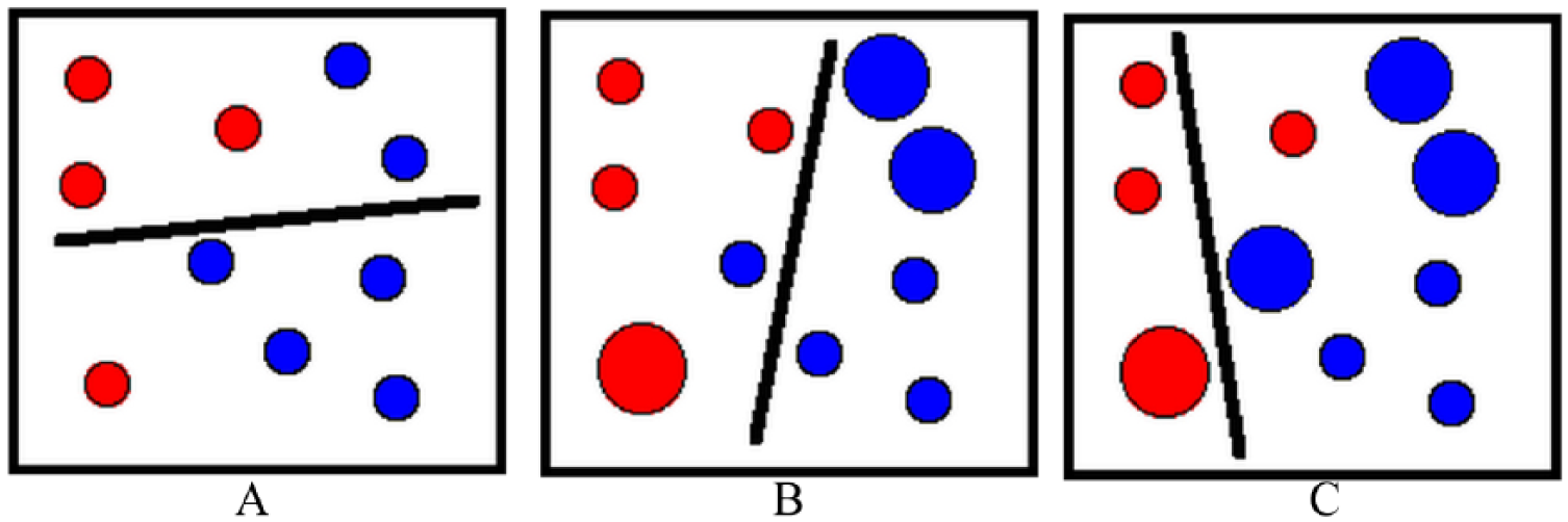
An example of the AdaBoost is illustrated in Figure 4. Red and blue circles represent 2 different classes. The algorithm starts with equal weights for each observation in the training set at iteration $t = 1$ (Figure 4A). For $D_{1}$ , the algorithm creates a weak classifier $h_{1}$ , which is represented by the line separating the 2 classes. Based on the results of the weak classifier $h_{1}$ , the algorithm updates the weights of the observations where misclassified observations are given higher weights. For $D_{2}$ , another weak classifier is created and weights are updated (Figure 4B). In this example, the total number of iterations is 3, ie, $T = 3$ . Hence, the final classifier is $H (x) = s i g n (α_{1} h_{1} (x) + α_{2} h_{2} (x) + α_{3} h_{3} (x))$ .

Figure 4.

Weak classifier for different iterations. (A) At iteration t = 1, a weak classifier is created for D1 where each observation has the same weight. (B) At iteration t = 2, after updating the weights of the observations, a new weak classifier is obtained for D2. (C) At iteration t = 3, final weak classifier is generated which is h₃.

To evaluate the performance of the model, we tested the model using cross-validation which is a general model validation technique for assessing how the prediction of a model will be generalized to an independent data set.³⁵ In this technique, data are separated into $k - f o l d s$ , where $k$ is less than or equal to the number of observations in the data set. Then, one of the folds is kept as the test set, and the rest of the folds are used for training the model. This process is replicated for each fold in the data, ie, $k$ times. The process is illustrated in Figure 5. In this study, we used 10-fold cross-validation and repeated the 10-fold cross-validation 10 times to eliminate the bias and overfitting the data.

Figure 5.

Illustration of $k - fold$ cross-validation.

Results

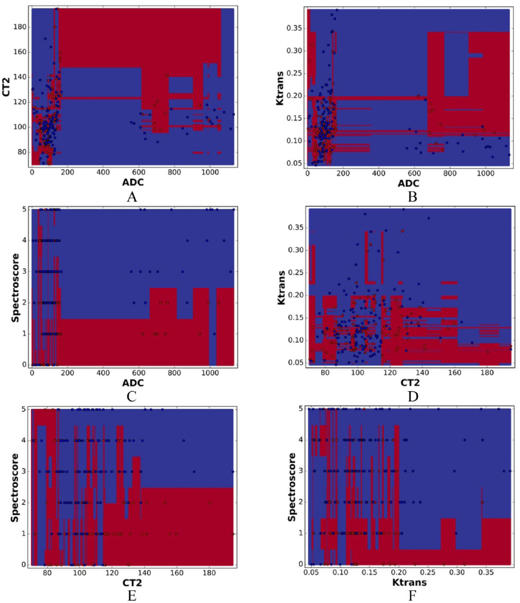
After testing the average and standard deviation of different percentiles (eg, 5th, 10th, 50th, 90th, and 95th percentiles) of the 4 imaging features, the average of the 50th percentile features performed the best. These 4 features were used to demonstrate the results. To separate aggressive prostate cancer (GS > 6) from indolent disease (GS ⩽ 6), we created models using 2 features at a time. Figure 6 shows the probability obtained from the classifiers for 6 possible combinations of the 4 imaging features. Using Figure 6A as an example, an adaptive boost model was created with ADC and $T_{2}$ values. Aggressive prostate cancer and indolent disease observations are represented with red and blue, respectively. Any point in the 2-dimensional space is shown with red, blue, or combination of red and blue based on the probability given by the classifier. Then, the decision boundaries for the aggressive prostate cancer (red) and indolent disease (blue) were obtained considering the probabilities (Figure 7). The final classifier separated 2-dimensional space into blue and red regions. For example, in Figure 7B, given ADC and $T_{2}$ values, the classifier predicts the aggressiveness of the cancer based on the color of the region that a point falls into. In the figure, the actual observations are shown as well.

Figure 6.

Probability from AdaBoost representing aggressive prostate cancer (red) and indolent disease (blue) using combinations of 2 imaging features. (A) ADC and T2, (B) ADC and K^trans, (C) ADC and Spectroscore, (D) T2 and K^trans, (E) T2 and Spectroscore, (F) K^trans and Spectroscore.

Figure 7.

Classifiers separating aggressive prostate cancer (red) and indolent disease (blue) from AdaBoost using combinations of 2 imaging features. A) ADC and T2, (B) ADC and K^trans, (C) ADC and Spectroscore, (D) T2 and K^trans, (E) T2 and Spectroscore, (F) K^trans and Spectroscore.

Figures 8 and 9 show the quantitative results of our methods from repetitions of 10-fold cross-validations. For distinguishing aggressive prostate cancer versus indolent disease (Figure 8), the averages and corresponding 95% confidence intervals of AUC, sensitivity, specificity, positive predictive value (PPV), and negative predictive value (NPV) were 0.73 (0.72-0.74), 0.72 (0.71-0.73), 0.73 (0.71-0.75), 0.34 (0.33-0.37), and 0.93 (0.92-0.94), respectively. For cancer foci detection (Figure 9), ie, classification between the absence of cancer (GS = 0) and presence of cancer (GS > 0), the averages and corresponding 95% confidence intervals of AUC, sensitivity, specificity, NPV, and PPV were 0.68 (0.66-0.70), 0.73 (0.70-0.77), 0.62 (0.60-0.68), 0.73 (0.71-0.76), and 0.65 (0.62-0.68), respectively.

Figure 8.

Summary of prostate cancer aggressiveness classification accuracy from 10 runs of 10-fold cross-validations showing average and 95% confidence intervals of AUC, sensitivity, specificity, PPV, and NPV.

Figure 9.

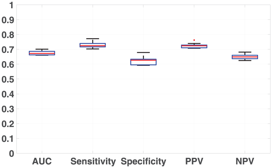
Summary of prostate cancer foci detection accuracy from 10 runs of 10-fold cross-validations showing average and 95% confidence intervals of AUC, sensitivity, specificity, PPV, and NPV.

Discussion

The current methods for prostate cancer diagnosis include PSA testing and transrectal biopsy. However, the accuracy of PSA testing is low with sensitivity around 20% for detecting any prostate cancer and around 50% for detecting high-grade prostate cancers.³⁶ However, biopsy is more reliable for prostate cancer diagnosis than PSA testing, but it is an invasive method. In a recent study, the reliability of a 12-core biopsy for prostate cancer detection was evaluated.⁴ For patients with <4 ng/mL, (4-10) ng/mL and >10 ng/mL PSA levels, the sensitivities were 40%, 63%, and 76%, respectively. The average sensitivity for the whole test group was 59%. We provided a noninvasive supervised learning tool using multiparametric MRI/MRSI that achieved an average sensitivity of 73% compared with PSA and biopsy.

When attempting to predict prostate cancer aggressiveness, previous studies excluded noncancerous observations (GS = 0). In this study, we included these observations while predicting the prostate cancer aggressiveness. Although this turned the classification problem difficult (as seen in Figure 6, the positive class [GS > 6] and the negative class [GS ⩽ 6] are very close to each other), it is more realistic and we were able to achieve an average AUC of 0.73 for prostate cancer aggressiveness prediction.

A potential limitation of this study is that all our data were from patients with prostate cancer and we did not have healthy prostate data as control. However, many specimens were not cancerous (Figure 1). We tested the correlation between the GS of adjacent specimens. The correlation coefficient was 0.3. The correlation coefficient for specimens that were one more slice apart was 0.004. Therefore, it was a valid assumption to treat specimens as independent observations. We plan to include healthy prostate data in the future to test our tool.

It was critical to be able to handle class imbalance when predicting prostate cancer aggressiveness. In practice, aggressive cancer only represents a small portion of the whole prostate. However, it is very important for the clinicians to be able to identify the aggressive cancer so that personalized treatment can be given. Dealing with class imbalance is still an ongoing research topic in machine learning field. And there were few studies which addressed this issue in prostate cancer prediction. In this study, the number of observations in one class (GS ⩽ 6) significantly outnumbered the other class (GS > 6) with the ratio of 5:1 (187/36). We demonstrated that our method of using undersampling in AdaBoost model was an effective way of handling class imbalance for prostate cancer aggressiveness prediction.

After prostate cancer diagnosis, many types of treatments are available including radiotherapy, endocrine therapy, surgery, etc. For men diagnosed with aggressive cancer, the goal is to keep the disease from spreading. Physicians can treat these patients with localized therapies such as surgery and radiotherapy. And systemic treatments, such as hormonal therapy, can also be used for these patients. A recent study shows that a mix of different treatments improves survival of patients with Gleason 9 and 10.³⁷ If aggressive prostate cancer can be identified early using the tools provided in this work, these types of treatment can be considered by physician.

Conclusions

Our results on both cancer foci detection and aggressiveness classification problems showed that using multiparametric MRI/MRSI with machine learning method could provide clinicians a more accurate predictive tool for prostate cancer assessment. Adaptive boosting with random undersampling could accurately identify highly aggressive prostate cancer. This noninvasive method will allow for nonsubjective disease characterization, which provides physician information to make personalized treatment decisions.

Footnotes

Funding:

The author(s) disclosed receipt of the following financial support for the research, authorship, and/or publication of this article: This work was supported in part by US Department of Defense through the grant number W81XWH-04-1-0249.

Declaration of conflicting interests:

The author(s) declared no potential conflicts of interest with respect to the research, authorship, and/or publication of this article.

Author Contributions

GK built the supervised machine learning tool and led the analysis of the prediction results and the writing of the manuscript. RG and WD interpreted the clinical significance of the results. GMDI analyzed the results and generated the figures. MN, JW, and NM processed the MRI images and collected the T2W, DWI-MRI and MRSI data. JP provided the histology on the data and the pathology interpretation. SR performed the octant work and collected the DCE-MRI data. RG, WD, and HZ conceived and designed the overall study. HZ designed the predictive modeling framework, supervised GK in developing the supervised machine learning tool, provided intellectual input, and participated in analyzing and interpreting the results. All authors were involved in either drafting or revising the manuscript and all authors approved the final manuscript.

References

American Cancer Society. Cancer Facts & Figures. Atlanta, GA: American Cancer Society; 2017.

Etzioni

Gulati

Tsodikov

et al . The prostate cancer conundrum revisited: treatment changes and prostate cancer mortality declines. Cancer. 2012;118:5955–5963.

Thompson

Pauler

Goodman

et al . Prevalence of prostate cancer among men with a prostate-specific antigen level ⩽4.0 ng per milliliter. N Engl J Med. 2004;350:2239–2246.

Chou

Croswell

Dana

et al . Screening for prostate cancer: a review of the evidence for the US preventive services task force. Ann Intern Med. 2011;155:762–771.

Schröder

Hugosson

Roobol

et al . Screening and prostate-cancer mortality in a randomized European study. N Engl J Med. 2009;360:1320–1328.

Andriole

Crawford

Grubb III

et al . Mortality results from a randomized prostate-cancer screening trial. N Engl J Med. 2009;360:1310–1319.

Serefoglu

Altinova

Ugras

Akincioglu

Asil

Balbay

MD.

How reliable is 12-core prostate biopsy procedure in the detection of prostate cancer?

Can Urol Assoc J. 2013;7:E293.

Turkbey

Kruecker

et al . Documenting the location of systematic transrectal ultrasound-guided prostate biopsies: correlation with multi-parametric MRI. Cancer Imaging. 2011;11:31–36.

Mottet

Bellmunt

Bolla

et al . EAU-ESTRO-SIOG guidelines on prostate cancer. Part 1: screening, diagnosis, and local treatment with curative intent. Eur Urol. 2017;71:618–629.

10.

Cooper

Merritt

Ross

John

Jorgensen

CM.

To screen or not to screen, when clinical guidelines disagree: primary care physicians’ use of the PSA test. Prev Med. 2004;38:182–191.

11.

Durmus

Baur

Hamm

Multiparametric magnetic resonance imaging in the detection of prostate cancer. Aktuelle Urologie. 2014;45:119–126.

12.

Delongchamps

Rouanne

Flam

et al . Multiparametric magnetic resonance imaging for the detection and localization of prostate cancer: combination of T2-weighted, dynamic contrast-enhanced and diffusion-weighted imaging. BJU Int. 2011;107:1411–1418.

13.

Lim

Kim

Cho

K-S.

Prostate cancer: apparent diffusion coefficient map with T2-weighted images for detection—a multireader study. Radiology. 2009;250:145–151.

14.

Donati

Afaq

Vargas

et al . Prostate MRI: evaluating tumor volume and apparent diffusion coefficient as surrogate biomarkers for predicting tumor Gleason score. Clin Cancer Res. 2014;20:3705–3711.

15.

Anwar

SSM

Anwar Khan

Hamid

et al . Assessment of apparent diffusion coefficient values as predictor of aggressiveness in peripheral zone prostate cancer: comparison with Gleason score. ISRN Radiol. 2014;2014:263417.

16.

Dianat

Carter

Macura

KJ.

Performance of multiparametric magnetic resonance imaging in the evaluation and management of clinically low-risk prostate cancer. Urol Oncol. 2014;32: 39.e1–39.e10.

17.

Fennessy

McKay

Beard

Taplin

M-E

Tempany

CM.

Dynamic contrast-enhanced magnetic resonance imaging in prostate cancer clinical trials: potential roles and possible pitfalls. Trans Oncol. 2014;7:120–129.

18.

Gillies

Morse

DL.

In vivo magnetic resonance spectroscopy in cancer. Annu Rev Biomed Eng. 2005;7:287–326.

19.

Haider

Van Der Kwast

Tanguay

et al . Combined T2-weighted and diffusion-weighted MRI for localization of prostate cancer. Am J Roentgenol. 2007;189:323–328.

20.

Oto

Kayhan

Jiang

et al . Prostate cancer: differentiation of central gland cancer from benign prostatic hyperplasia by using diffusion-weighted and dynamic contrast-enhanced MR imaging. Radiology. 2010;257:715–723.

21.

Anderson

Golden

Wasil

Zhang

Predicting prostate cancer risk using magnetic resonance imaging data. Inform Syst e-Business Manag. 2015;13:599–608.

22.

Abd-Alazeez

Kirkham

Ahmed

et al . Performance of multiparametric MRI in men at risk of prostate cancer before the first biopsy: a paired validating cohort study using template prostate mapping biopsies as the reference standard. Pros Cancer Pros Dis. 2014;17:40–46.

23.

Fehr

Veeraraghavan

Wibmer

et al . Automatic classification of prostate cancer Gleason scores from multiparametric magnetic resonance images. Proc Nat Acad Sci. 2015;112:E6265–E6273.

24.

Langer

van der Kwast

Evans

Trachtenberg

Wilson

Haider

MA.

Prostate cancer detection with multi-parametric MRI: logistic regression analysis of quantitative T2, diffusion-weighted imaging, and dynamic contrast-enhanced MRI. J Mag Reson Imaging. 2009;30:327–334.

25.

Japkowicz

Stephen

The class imbalance problem: a systematic study. Intel Data Anal. 2002;6:429–449.

26.

Weiss

GM.

Mining with rarity: a unifying framework. ACM SIGKDD Explor Newslett. 2004;6:7–19.

27.

Sun

Kamel

Wong

Wang

Cost-sensitive boosting for classification of imbalanced data. Patt Recogn. 2007;40:3358–3378.

28.

Estabrooks

Japkowicz

A multiple resampling method for learning from imbalanced data sets. Comput Intel. 2004;20:18–36.

29.

Chawla

Bowyer

Hall

Kegelmeyer

WP.

SMOTE: synthetic minority over-sampling technique. J Artif Intel Res. 2002;16:321–357.

30.

Drummond

Holte

RC.

C4.5, class imbalance, and cost sensitivity: why under-sampling beats over-sampling. Paper presented at Workshop on learning from imbalanced datasets II, vol. 11; Washington, DC; August 21, 2003.

31.

Liu

X-Y

Zhou

Z-H.

Exploratory undersampling for class-imbalance learning. IEEE T Syst Man Cy B. 2009;39:539–550.

32.

Tofts

Brix

Buckley

et al . Estimating kinetic parameters from dynamic contrast-enhanced T(1)-weighted MRI of a diffusable tracer: standardized quantities and symbols. J Magn Reson Imaging. 1999;10:223–232.

33.

Schapire

RE.

Explaining AdaBoost. In: Schölkopf

Luo

Vovk

, eds. Empirical Inference. New York, NY: Springer; 2013:37–52

34.

Freund

Schapire

RE.

A decision-theoretic generalization of on-line learning and an application to boosting. In: Vitányi

PMB

, ed. European Conference on Computational Learning Theory. London, England: Springer; 1995:23–37.

35.

Kohavi

A study of cross-validation and bootstrap for accuracy estimation and model selection. In: Proceedings of the 14th International Joint Conference on Artificial Intelligence, vol. 14. Stanford, CA: Morgan Kaufmann Publishers; 1995:1137–1145.

36.

Wolf

Wender