Sage Journals: Discover world-class research

Abstract

Exon capture across species has been one of the most broadly applied approaches to acquire multi-locus data in phylogenomic studies of non-model organisms. Methods for assembling loci from short-read sequences (eg, Illumina platforms) that rely on mapping reads to a reference genome may not be suitable for studies comprising species across a wide phylogenetic spectrum; thus, de novo assembling methods are more generally applied. Current approaches for assembling targeted exons from short reads are not particularly optimized as they cannot (1) assemble loci with low read depth, (2) handle large files efficiently, and (3) reliably address issues with paralogs. Thus, we present Assexon: a streamlined pipeline that de novo assembles targeted exons and their flanking sequences from raw reads. We tested our method using reads from Lepisosteus osseus (4.37 Gb) and Boleophthalmus pectinirostris (2.43 Gb), which are captured using baits that were designed based on genome sequence of Lepisosteus oculatus and Oreochromis niloticus, respectively. We compared performance of Assexon to PHYLUCE and HybPiper, which are commonly used pipelines to assemble ultra-conserved element (UCE) and Hyb-seq data. A custom exon capture analysis pipeline (CP) developed by Yuan et al was compared as well. Assexon accurately assembled more than 3400 to 3800 (20%-28%) loci than PHYLUCE and more than 1900 to 2300 (8%-14%) loci than HybPiper across different levels of phylogenetic divergence. Assexon ran at least twice as fast as PHYLUCE and HybPiper. Number of loci assembled using CP was comparable with Assexon in both tests, while Assexon ran at least 7 times faster than CP. In addition, some steps of CP require the user’s interaction and are not fully automated, and this user time was not counted in our calculation. Both Assexon and CP retrieved no paralogs in the testing runs, but PHYLUCE and Hybpiper did. In conclusion, Assexon is a tool for accurate and efficient assembling of large read sets from exon capture experiments. Furthermore, Assexon includes scripts to filter poorly aligned coding regions and flanking regions, calculate summary statistics of loci, and select loci with reliable phylogenetic signal. Assexon is available at https://github.com/yhadevol/Assexon.

Keywords

Exon capture read assembly de novo assembly data filtering phylogenomics hybrid enrichment

Introduction

Both empirical and theoretical studies show that intensely sampled unlinked loci can improve the estimation genetic parameters of populations^1,2 and resolve conflicts in phylogenetic inference.^3,4 Whole genome sequencing can be used for phylogenomic analyses,⁵ but it is still unaffordable at large scale. Combining next-generation sequencing (NGS) and target enrichment is one of the efficient ways to collect plentiful loci across various taxonomic divergence.^6-9 Studies have been focused on collecting conserved sequences that can be reliably captured across divergent taxa for phylogenomic analysis, including ultra-conserved elements (UCEs), anchored elements,^7,10,11 conserved coding, and non-coding regions.^12-14 The targeted sequences are enriched by hybridizing RNA oligonucleotide probes (aka “baits” designed from transcriptomes or existing genomes) to homologous regions of the targeted taxa, which are subsequently isolated and pooled for sequencing. Exons are among the most well-studied and modeled parts of the genome and are generally more conserved than introns, resulting in consistent capture across divergent taxa, and thus they have been one of the promising markers for phylogenomic studies through target enrichment.^8,9,15 However, to date, approaches for de novo assembly of exons from short-read raw sequence data have not be optimized.

Streamlined pipelines have been developed for UCEs and Hyb-seq data, represented by PHYLUCE¹⁶ and HybPiper,¹⁷ respectively. PHYLUCE directly inputs the entire set of short reads into assembler to assemble them into contigs. Then, contigs are parsed to homologous loci. When dealing with large numbers of loci (>10 000), computer memory becomes a major limiting factor for simultaneous de novo assembly of raw reads pooled across loci. HybPiper is able to extract exonic and intronic regions from Hyb-seq data from raw sequence reads, but its assembler (multi-cell mode of SPAdes)¹⁸ cannot assemble loci with low read depth (<10×). Nonetheless, read depth for short loci or for data from capturing divergent taxa tends to be low, which may cause problems in read assembly using HybPiper.

Another major problem in assembling loci for phylogenomic analysis is the challenge of identifying and excluding paralogous loci after assembly. Including undetected paralogs often leads to discordance between gene trees and species trees.¹⁹ Targeting putatively single-copy loci can help to reduce the incidence of enriching paralogs.²⁰ However, additional checks are still necessary to preclude mistakes in the assemblies. Current pipelines either simply ignore verification of orthologs^21,22 or do not use information from reference genomes to check on paralogs. For example, in PHYLUCE, each reference sequence of the target loci is compared to the assembled contigs. An assembled contig is accepted as orthologous if it is the only hit for a given locus of reference sequence, and also no other target locus has a hit on the same contig. This could be problematic because more than one contig has a hit on the reference sequence of the target when non paralog exists. For example, loci sometimes cannot be fully assembled, which could result in multiple contigs. Thus, we would lose some orthologous loci if we discard them all. Moreover, the orthologous copy of the locus may be lost or not enriched in the experiment, so we may mistakenly accept a paralog as the orthologous sequence. An alternative approach would be to compare the assembled contig to the whole genome that the baits were designed from, or a genome of species that is closely related to the target taxa, as a reference to evaluate all potential matches and determine if it is the orthologous copy of the target locus.

Flanking sequences often are captured through hitchhiking in addition to targeted exon regions. Flanking sequences are available in the results from most read assembling pipelines for exon capture data, but they were seldom incorporated into phylogenetic analysis (but see Yuan et al²³ and Bi et al²⁴), because some flanking regions are too variable to be aligned. Nonetheless, discarding all flanking sequences may miss useful data for investigating population histories or phylogenetic relationships between recently diverged taxa. Filtering flanking sequences of exonic regions for useful data should be incorporated in the pipelines for read assembling designed for exon capture data.

Undetected paralogs, mis-assemblies, or missing data may result in poorly aligned regions of sequence alignments. These regions could mislead phylogenetic inferences, so data filtering should be a crucial final step in read assembly. In commonly used pipelines, this step is either absent (eg, HybPiper) or sequences are filtered based on simple statistics such as p-dist is applied (eg, PHYLUCE). More sophisticate filtering methods could be developed for controlling the quality of alignments, such as removing loci that are randomly aligned.^25,26 Filtering loci based on whether their gene tree agrees with widely accepted phylogenetic relationship (eg, known monophyletic groups) or other criteria (eg, fit a molecular clock)²⁷ may also be helpful.

In order to address problems mentioned above, we designed Assexon (assembling exons), a streamlined pipeline to turn short reads from exon capture experiments into sequence alignments ready for phylogenomic analyses. Assexon has 3 phases: data preparation, read assembly, and post-assembly processing. In data preparation steps, reads are deduplicated and parsed to target loci according to their similarity to the reference loci. Parsing reads before de novo assembling can increase efficiency of assembling sequences from large read files. In post-assembly processing steps, recovered sequences are compared against a reference genome to reduce the risk of retrieving paralogs. Assexon includes scripts to remove poorly aligned flanking sequences and use alignable data in the flanking regions. Assexon also comprises filters to select loci with reliable phylogenetic signal. We evaluated performance of Assexon by comparing it to commonly used pipelines. Assexon is aimed to assemble data produced from cross-species exon capture; thus, mapping-based targeted assembling pipelines, such as Mapsembler²⁸ and TASR,²⁹ are not included in the comparison. We selected 3 targeted read assembling pipelines specifically designed for cross-species exon capture data, including PHYLUCE, HybPiper, as well as a custom exon capture analysis pipeline from Yuan et al,²³ abbreviated as “CP” hereafter.

Materials and Methods

Assexon is a suite of scripts written in Perl and wrapping around several bioinformatics tools. Assexon consists of 3 parts: data preparation, read assembly, and post-assembly processing. Read assembly was scripted in modules, so to allow users to rerun portions of the pipeline.

The input of Assexon includes paired-end reads in FASTQ format, a reference genome, and exon marker sequences that are extracted from reference genome and used to design baits in FASTA format. The genome sequences are used for identifying paralogs. If sequences of multiple genomes from various species are used to design markers, all genome sequences are required to be concatenated into a single file. The marker sequences are used as a reference during assembly. If coding frames of reference are not determined, known protein sequences of reference species and an index file are required for prediction of coding frames. Known protein sequences of reference species could be generally downloaded from public database like Ensembl.³⁰ Index file is generated from Evolmarkers.³¹ It comprises the name of each reference sequence and corresponding known protein sequence ID of each reference sequence, which can help to find protein sequences of each reference sequence from file of known protein sequences. On the contrary, known protein sequences and index file are not required to be provided if coding frames can be determined by alternative approaches, such as using transcriptome data to find the coding frames.

Data preparation

The pipeline starts with trimming low-quality bases and sequence adaptors using trim_galore v0.4.1 (http://www.bioinformatics.babraham.ac.uk/projects/trim_galore/). Coding frame of each marker sequence is predicted and corrected using a Perl script (predict_frames.pl). It first checks the translated reference sequences of the 3 frames for stop codons and eliminating any frames that contain inappropriately placed stop codons. Known protein sequences of reference are retrieved from file of known protein sequences and aligned with translated protein sequences to find the correct frame. Finally, coding sequences are extracted and translated into amino acid sequences using Bio::Seq module in Bioperl.³²

Read assembly

General pipeline workflow of read assembly is shown in Figure 1 and detailed implementation is described below.

Figure 1.

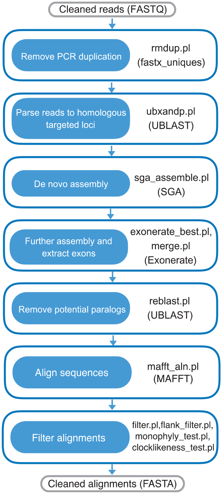
Outline of assembling procedure. (1) PCR duplications are removed from trimmed reads using rmdup.pl. (2) De-duplicated reads are parsed to homologous loci using ubxandp.pl. (3) Parsed reads are separately assembled into contigs using sga_assemble.pl. (4) Contigs are elongated and then exons are extracted from contigs with best hit to references using exonerate_best.pl and merge.pl. (5) Potential paralogs are removed using reblast.pl. (6) Resulting assemblies are aligned using mafft_aln.pl. (7) Alignments can be filtered using filter.pl, flank_filter.pl, monophyly_test.pl, or clocklikeness_test.pl.

Remove PCR duplication

Duplicate reads are generated during the steps of polymerase chain reaction (PCR) in library construction and exon capture. They are redundant and may lower the efficiency of reads parsing and assembly, so it is necessary to remove PCR duplication first. Size of input reads from exon capture could be large, so de-duplicating entire dataset at once may be computationally demanding. First, paired reads are concatenated into super-reads and then the first “k” bases of the super-reads are taken as prefix. Reads with the same prefix are clustered together, which make PCR duplicates not be spread over to different clusters. Size of each cluster is around m (m = 200 Mb). If the file size of concatenated reads is denoted as s, then k is calculated as

k = [\frac{\log ([\frac{s}{m}])}{\log (4)}]

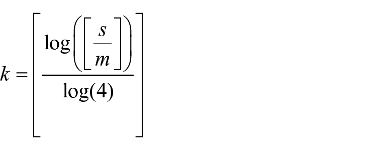
Eventually, each cluster is de-duplicated using “-fastx_uniques” command in USEARCH v10.0.240.³³ Duplication-free clusters are merged together and restored to paired reads.

Parsing reads to homologous targeted loci

Reads are parsed to targeted loci before assembling. This step could significantly reduce the complexity and improve the efficiency of assembly. To avoid including low-complexity reads from non-targeted region into the assembling process, low-complexity sequences in de-duplicated reads and in the sequences of targeted reference are soft-masked before parsing, which are done using DUST and Segmasker^34,35 implemented in USEARCH v10.0.240. Subsequently, reads are sorted to references with BLAST hit using UBLAST with a relaxed e-value of 1 × 10⁻⁴. Sorted reads are written to files of separated loci in FASTQ format using ubxandp.pl.

De novo assembly

Multiple edges could be connected to the same node in assembly graph, which could be resulted from gene copies, alleles, or sequencing errors.³⁶ Current assemblers like Velvet³⁷ and Abyss³⁸ choose edges with higher read support or depth. However, read depth tends to be low for short loci or when targeted loci of samples are divergent from baits in exon capture, so it is hard to choose a correct edge depending only on read depth. A conservative assembler is required, which does not arbitrarily choose the edge according to read depth, but aligns resulting contigs to references and selects the edge that has higher alignment score to reference. SGA³⁹ was chosen to assemble reads of each locus into contigs, which is a conservative but accurate assembler. It disallows any conflicting edges that connect to the same node in the string graph if divergence between edges is more than 5%. Graph is separated from the nodes that connect with multiple edges. Overlapping information between contigs are available from the output of SGA, which are used to reconstruct overlapping graph and help to reduce conflicting edges in next step. Minimum overlap and maximum error rate (denoted as e) allowed between contigs are 25 bp and 0.05, respectively. The “filter” command in SGA extracts k-mers (k = 27 in default) from reads and then removes reads with low k-mer frequencies (<3) before assembly, which could induce erroneous edges. We disable this function for the loci whose file size of input reads are below 500 Kb, to avoid loss of these loci due to low read depth.

Further assembly and extract candidate exons

Multiple edges could be left in the string graph of the preliminary assembly. We need to reduce the conflicting edges and extract candidate exons in this step. Contigs are locally aligned to protein sequences of references using the “protein2dna” model in the package under Exonerate⁴⁰ to get their positions to the reference and alignment score, which are used to determine the short overlap between contigs (shorter than 25 bp but longer than 10 bp) and reduce conflicting edges. Two contigs are regarded as having overlaps if their positions to reference are crossed. However, some of the contigs could be accidentally aligned in a crossed position, but they are not truly overlapped. It could be too slow to find exact overlap for each pair of contigs in the following step, if too many pairs of contigs that are not truly overlapped are included. To primary screen out false overlaps, k-mers are extracted from overlapped region of contigs, and the number of matched k-mer is compared with minimum possible number of matched k-mer between overlaps with given length. We do not know the length of the exact overlap, so we define an “ambiguous overlap,” which is close to the exact one. Ambiguous overlap consisted of crossed region, unaligned bases at the end of the first contig, and unaligned bases at the start of next contig. Substitutions, indels, or sequencing error may occur at the both ends of contigs, so these bases cannot be aligned to reference. We add them into ambiguous overlap because these bases may exist in the true overlap. Figure 2 shows the diagram of ambiguous overlap between contigs. We consider that contigs probably have true overlap if ambiguous overlaps are longer than 5 bp. Then, k-mers (k = 5) are extracted from ambiguous overlaps of the contigs. If we denote length of ambiguous overlap and maximum error rate allowed between overlapped sequences as l and e, respectively, minimum possible number of matched k-mer (denoted as “min(m)”) required between them is

m i n (m) = {\begin{matrix} l - k + 1 - [e \times l] \times k i f m i n (m) > 0 \\ 1 i f m i n (m) \leq 0 \end{matrix}

Figure 2.

Diagram of ambiguous overlap between 2 contigs. Green and black lines represent reference and overlapped contigs. Blue dashed lines represent unaligned bases. Substitutions occur at the bases neighboring to the crossed region, so they cannot be aligned to reference. Ambiguous overlap consisted of crossed region, unaligned bases at the end of contig 1, and unaligned bases at the start of contig 2 in this diagram.

Then, we find exact overlaps from filtered overlaps by comparing the end of first contig with the start of next contig. Overlap graphs are reconstructed based on these overlaps and the ones extracted from graph files. Conflicted paths are reduced by selecting paths with the highest alignment score to reference. Only conflicted edges in coding regions can be reduced, because they are covered by references, however, conflicted edges in flanking regions still remain. We traverse through the graphs and retrieve all possible paths that are aligned to protein sequences of references with “protein2dna” model. We select sequences that are aligned with more than 80% of reference sequences and have at least 60% of similarity to references. Finally, we only retrieve one of the selected sequences with top alignment score as candidate. Part of sequences embedded in the alignment boundaries are retrieved as exons and rest of them are treated as flanking sequences.

Remove potential paralogs

In order to verify the orthology of retrieved sequences, BLASTn is performed to align candidate sequences against reference genome using UBLAST. Sequences are classified as potential paralogs, if their best BLAST hit do not overlap with the targeted regions in the genome, and discarded before downstream analysis.

All steps mentioned above were individually scripted and called through a wrapper (assemble.pl). Typically, users could run through all phases as a single pipeline, or alternatively, portions of the pipeline can be rerun individually to test various parameters. Output from the last step includes 3 FASTA files for each locus: coding sequences with and without flanking regions, and protein sequences for the coding sequences. Basic statistics are summarized including number of bases and reads in trimmed and de-duplicated reads, number and percentage of enriched loci for each sample. Users can assess performance of enrichment through these statistics.

Post-assembly processing

Dataset manipulation and aligning

Assexon includes scripts to flexibly manipulate the dataset. A subset of taxa can be extracted using pick_taxa.pl, which can also select loci with various levels of completeness. If genome sequences of taxa outside of targeted samples are available, get_orthologues.pl can be used to retrieve orthologous sequences to the reference loci, so extracted sequence can be added into files of enriched loci using merge_loci.pl. After preparing the datasets, each targeted locus is aligned using MAFFT, which is paralleled using mafft_aln.pl. Coding sequences are translated and then aligned based on protein sequences. Flanking sequences are non-coding, so sequences with flanks need to be aligned in nucleotide with “–non_codon_aln” option.

Data filtering

Poor alignments could interfere phylogenetic inference, so we designed filter.pl to remove badly aligned sequences in coding regions. Sequences having long insertion or deletions (⩾10 bp) with respect to reference are removed, which rarely occur in coding regions. A 50 bp sliding window with 25 bp per step is applied to scan alignment subsequently. Sequence is discarded if at least one of the sequences across windows is distant from the reference (p-dist ⩾ 0.4). Notably, entire sequences are removed instead of partial sequences in the sliding to keep the intactness of coding region. Finally, only alignments having length of at least 100 bp, and sequences that cover more than 80% of alignments length are retained.

Poorly aligned flanking sequences are removed using flank_filter.pl. Flanks need to be trimmed to similar length, so that there is not much missing data at both ends. Flanks are trimmed from each ends until at least 5 successive columns having more than 50% of nucleotides are found. Sequences having short insertions (⩾10 bp) are removed from flanks, which could lead to non-homologous alignment and lots of gaps in flanks. After cleaning up regions with lots of missing data, unalignable data in flanks must be removed. Similar long sequences could be inserted in some of the intronic flanks of closely related samples.⁴¹ Because the length of enriched flanking region is limited in the exon capture experiments, it is likely that only partial insertions could be enriched in flanks. These insertions are too diverged to be aligned with other flanking sequences without the insertion, so one must keep either the group of sequences with insertions or without insertions. Pair of distant flanks is selected if p-dist between them exceeds 0.4. Then, average p-dist of 2 flanks to the rest of the taxa are computed. The flank sequences that are more distant to the rest of the taxa are removed. We iterate this process until there are no pairs of distant sequences in flanking regions. Comparing with the coding region, there are more sequences that are locally diverged from other sequences in flanking region. To aggressively remove those sequences, a stricter window (20 bp, 10 bp per step) is used to slide through the flanks. Sequences are trimmed from the window that is the nearer to the coding region to the ends, if at least one sequence across window are too diverged from alignment consensus (p-dist ⩾ 0.4). Finally, only flanking blocks having at least 65% of input taxa and sequences covering at least 65% of the length of flanking alignments are possessed.

Furthermore, scripts to screen out loci based on pre-defined monophyletic groups are provided in Assexon, which could be very helpful when users have knowledge about studied groups (monophyly_test.pl). It is too rigorous to merely pick out loci whose topologies of gene trees strictly follow the given monophyletic groups due to stochastic process of genealogy. Thus, we build a maximum likelihood (ML) tree constrained with pre-defined groups for each locus and a ML tree with no constraint. Then, Shimodaira and Hasegawa (default) or Approximately Unbiased test implemented in PAUP* 4.0a164⁴² is applied to each locus, and we only select loci if there is no significant difference between their relaxed ML and constrained ML tree (P > .05). Clocklike loci can be selected using clocklikeness_test.pl, which computes the likelihoods of ML tree with given alignment of each locus when they are constrained with molecular clock or without using PAUP* 4.0a164. Loci are retained if there is no remarkable difference between likelihoods with and without molecular clock constraint (P > .05).

Other scripts

Summary statistics for coding and flanking region of each locus and sample can be extracted from alignments of coding and flanking regions using statistics.pl. Summarized statistics for the coding region of each locus include number of enriched samples, alignment length, GC content, percentage of missing data, and average pairwise distance among sequences. Summarized statistics for flanking regions of each locus include alignment length of flanking region and average pairwise distance. Summarized statistics for each sample include the number of enriched loci, GC content, and average length of the flanking region. Sequencing depth, number, and percentage of on-target reads for each sample are summarized from alignment between trimmed reads and assemblies using map_statistics.pl. Assexon also contains scripts to format filtered alignments as input of phylogenetic analysis including RAxML⁴³ and ASTRAL.⁴⁴ Single nucleotide polymorphism (SNP)-based analysis is frequently included in most of phylogenomic studies. To extract SNPs, first a majority-rule consensus reference (consensus.pl) is generated for each alignment, either with or without flanks. Then, an automatic workflow (gatk.sh) is used to map trimmed reads to consensus references using BWA v0.7.15-r1140,⁴⁵ PCR duplicates are marked using Picard MarkDuplicates (http://broadinstitute.github.io/picard/) and then SNPs are extracted across several samples following the best practices of germline short variant discovery recommendations^46-48 using GATK–3.4.0.⁴⁸ One qualified SNP from each loci is randomly selected to meet the assumption of linkage disequilibrium in phylogenetic analysis and rearranged into input of several prevalent SNP-based analysis software comprising STURCTURE,⁴⁹ dudi.pca under R package ade4⁵⁰ and BEAST⁵¹ using vcftosnps.pl.

Assess the performance of Assexon and other pipelines

PHYLUCE, HybPiper, and a custom pipeline (CP) developed by Yuan et al were selected. They are commonly used pipelines to assemble cross-species gene capture data. PHYLUCE was specifically designed to assemble data captured by baits that are designed based on UCEs. In PHYLUCE, first entire read set are assembled into contigs and then contigs are aligned with reference sequences to find the orthologous sequences of each locus. A contig is accepted as orthologous if it is the only hit for the given reference sequence. HybPiper was developed for Hyb-seq data, which is mostly captured by baits that are designed based on exon markers. In HybPiper, first paired reads are parsed to homologous loci, then reads of each locus is separately assembled. Assembled contigs are aligned with reference sequences, and Hybpiper identifies the full-length contigs that span more than 85% of the length of the reference sequences. A contig is recognized as orthologous if it is the only full-length contig with given reference sequence. If multiple full-length contigs are found, a read depth cut-off is used to choose contig. A contig is chosen if its read depth is at least 10 times greater than next best full-length contig. If read depths are close among full-length contigs, the contig with the highest similarity to reference sequences is chosen. CP was designed to assemble exon capture data. Similar to Assexon, CP first removes PCR duplication from raw reads and then reads are parsed to homologous loci. Each locus is individually assembled using the Trinity assembler⁵² and then further assembled using Geneious v7.1.5 (https://www.geneious.com). An assembly process normally includes multiple samples and each sample could comprise thousands of loci that need to be assembled, while only 2000 to 3000 loci can be assembled using Geneious v7.1.5 in a single run. Thus, users need to manually run Geneious v7.1.5 multiple times to further assemble all sequences. Method to extract exon and identify orthologous sequences in CP is almost the same as Assexon, except that CP uses Smith-Waterman algorithms to find the contig with the highest alignment score to reference. Performance of PHYLUCE, HybPiper, and CP to recover assemblies from exon capture data will be assessed and compared with the performance of Assexon.

Reads from 2 exon-capture experiments were collected to test the performance of Assexon and other pipelines. In experiment 1 (test 1), the species used to design baits (Lepisosteus oculatus) and the targeted species (Lepisosteus osseus) belonged to the same genus. In the other experiment (test 2), species used to design baits and targeted species, Oreochromis niloticus and Boleophthalmus pectinirostris, were from different orders of teleost fishes. Detailed information of the datasets is listed in Table 1. The trimmed data without adapters and low quality bases are lodged in GenBank with accession number PRJNA562564. Single-copy exon markers were extracted from annotated genomes of L oculatus, Danio rerio, Oryzias latipes, Gasterosteus aculeatus, Tetraodon nigroviridis, Anguilla japonica, Gadus macrocephalus, and O niloticus using Evolmarkers.³¹ Baits, in 120-bp length, were designed based on 13 843 and 17 817 sequences of L oculatus and O niloticus with 2× tiling according to the recommendation of manufacturer (MYcroarray, Ann Arbor, Michigan). The bait sequences less than 120 bp were padded with thymine at 3’ end to 120 bp. Biotinylated RNA baits were synthesized by MYcroarray. Information of markers and reference sequences can be found in Supplementary S2.

Table 1.

Summary statistics of cross-species and cross-order capture data.

	Species of sample	Trimmed reads (bp)^a	Species of reference targets (bp)	Number of target loci^b	Divergence time (Myr)^c	The closest species with genome available
Test 1	L osseus	1 659 770 753	L oculatus	13 843	3.2	L oculatus
Test 2	B pectinirostris	915 882 266	O niloticus	17 688	128	B pectinirostris

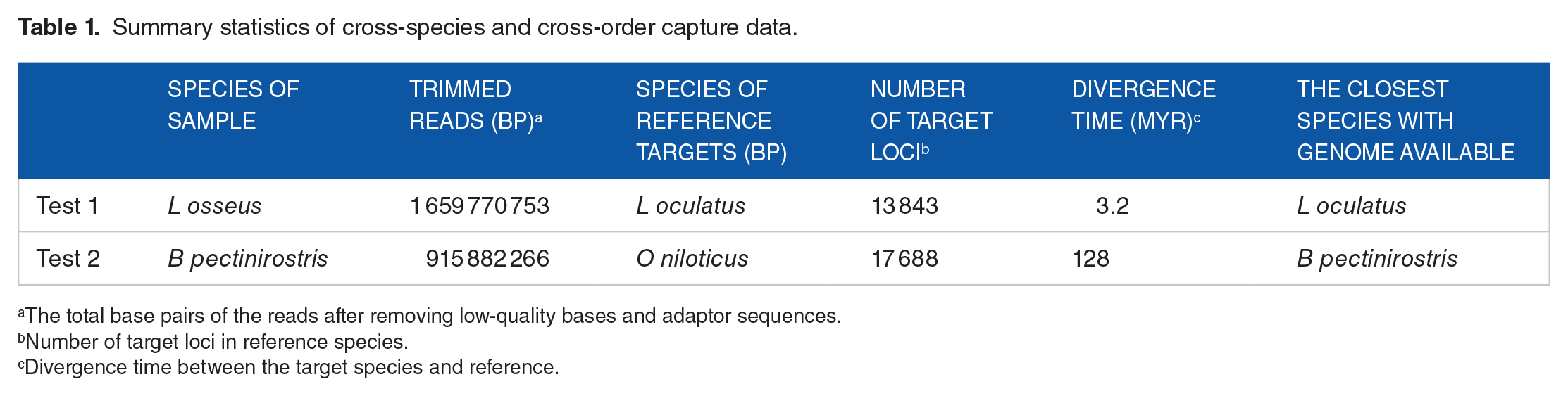
The total base pairs of the reads after removing low-quality bases and adaptor sequences.

Number of target loci in reference species.

Divergence time between the target species and reference.

Genomic DNA were sheared to 250 bp using Covaris (Covaris, Woburn, USA). Sheared DNA (350-500 ng) was used to construct libraries. Exon capture was performed following Li et al.¹² Custom adaptors with 8 index were used to discriminate reads of different samples. These 2 samples were pooled with other 98 samples from other projects in equimolar quantities for pair-ended sequencing on a Hiseq 2500 platform (Illumina, Inc, San Diego, CA, USA).

Raw reads were de-multiplexed to separated files based on 8 indices using BclToFastq (Illumina, Inc, San Diego, CA, USA). Remaining adaptors and low-quality bases were trimmed using trim_galore v0.4.1 with default parameter. Then, trimmed reads, sequences of reference and genome were fed into Assexon, PHYLUCE, HybPiper, and CP. Reads were assembled with default parameters in different tools, except that E-value for read sorting in HybPiper was set to 1 × 10⁻⁴ to keep the same setting as in Assexon and CP. Because CP was single threaded, it was run in single thread on a Linux cluster. Assexon, PHYLUCE, and HybPiper were executed in 12 threads on a Linux cluster.

Completeness and accuracy of assemblies in coding region was evaluated by comparing them to reference sequences and available genome sequences of species that are most closely related to targeted samples. Because reference sequences and assemblies in coding regions are generally in similar length, comparison between reference sequences and assemblies helps to evaluate the completeness of assemblies in coding region. Because species of genome sequences are the same species as targeted samples (in test 2) or very closely related to targeted samples (in test 1), its exonic sequences are almost the same as the ones in targeted samples. Thus, those genome sequences help to evaluate the accuracy of assemblies in coding region. Four metrics were extracted from comparison: similarity between assembled contig and reference (SAR), similarity between assembled contig and genome (SAG), coverage of assemblies to reference (CAR), and coverage of assemblies to genome (CAG). These metrics were used to divide assemblies into 3 classes: recovered, accurately assembled, and perfectly assembled. Recovered loci were defined as assemblies having at least 60% of SAR and 80% of PRA. A subset of recovered loci were considered as accurately assembled, if their aligned exons had at least 99% of SAG and 100% of CAG. Perfectly assembled loci were a subset of accurately assembled loci that have 100% of CAR. In test 1, as there was no existing genome of L osseus, sequences of L osseus were compared against the genomic sequences of L oculatus. In test 2, sequences of B pectinirostris were compared against genomic sequences of B pectinirostris from You et al.⁵³

Sequences were recognized as paralogs if they cannot be aligned to targeted regions in genomes. For each recovered paralog, reference sequence, orthologous sequence to reference in targeted species, recovered paralog, and sequence found in genome of reference that is orthology to paralog were collected and aligned. Phylogenetic trees were reconstructed using RAxML under GTRGAMMA model to further prove the paralogy between the reference and recovered sequence. Paralogy validation was not run in test 1, because no genome of L osseus is available.

In order to make precise comparison, assembling procedure of the 4 pipelines were further divided into 5 steps including removing PCR duplication, parsing reads to homologous loci, de novo assembly, extracting exons, and removing potential paralogs. Extracting exons and removing potential paralogs were performed simultaneously in PHYLUCE and HybPiper, so we categorized these 2 steps as “extract exons.” As one of the main purposes of fourth step of Assexon (further assembly and extract exon) is to extract exons from assemblies, we categorized it as “extract exons,” even it was also aimed for further assembly. Peak RAM usage and CPU time of each step was accessed separately using custom script (RAM_CPU_time.pl). PHYLUCE does not include the step of removing PCR duplication and parsing reads to homologous loci, and HybPiper does not comprise the step of removing PCR duplication, thus corresponding total CPU time and peak RAM usage were not available. RAM usage and CPU time of the further assembly step in CP could not be accessed, because this step needed to be manually operated.

Data from a previous study by Jiang et al⁵⁴ was also used to assess the performance of 4 pipelines to provide additional independent test. Detailed information of dataset and results can be found in Supplementary S1.

Variabilities in original and filtered flanking regions

In addition, we explored the variation in flanking regions at species and population level, and the capability of the script to remove poorly aligned flanks was evaluated. Trimmed raw reads of gene capture of 5 individuals of Siniperca chuatsi and another 5 of S kneri were selected from Song et al.¹⁵ Summary of sequencing statistics of 10 sinipercids is listed in Supplementary Table S1. Orthologous exons with and without flanks were recovered using Assexon. Then, they were aligned using mafft_aln.pl. Poorly aligned coding sequences were filtered using filter.pl. Unalignable flanks were removed using flank_filter.pl. A custom script (block_pdis.pl) was used to calculate p-dist between each taxa and average p-dist among all taxa from original and filtered flanks. p-dist of flanks were calculated if their length was at least 20 bp. Consensus sequence of each locus was generated from its filtered alignment with flanks using consensus.pl. Trimmed reads were subsequently mapped to consensus sequences. SNPs across 10 individuals of Siniperca were extracted from BAM files using gatk.sh. Number of SNPs in filtered coding and flanking regions were counted using a custom script (snp_num.pl). All custom Perl scripts can be found in Supplementary S3.

Results

Performance of exon assembly among 4 approaches of exon capture

We evaluated performance of exon assembly of Assexon, PHYLUCE, HybPiper, and CP by comparing number of recovered loci, accurately assembled loci, perfectly assembled loci, paralogs, peak RAM usage, and total CPU time.

Number of loci assembled using 4 pipelines

The number of loci assembled using 4 pipelines is listed in Table 2. For number of recovered loci, approximately 12 000 loci were assembled using Assexon (12 064) and CP (11 823) in test 1, which were almost twice as many as loci produced using PHYLUCE (6900). The number of loci recovered using HybPiper was 9356. As species used for bait design and targeted species are phylogenetically diverged, number of recovered loci significantly decreased in test 2. About 6800 loci were recovered using Assexon (6830) and CP (6891), which were almost 3 times more than using PHYLUCE (2382). The number of loci in test 2 recovered using HybPiper was 4205 loci.

Table 2.

Number of recovered, accurately assembled, perfectly assembled loci, and paralogs produced using 4 pipelines in 2 tests.

	Pipelines	Recovered loci (%)	Accurately assembled loci (%)	Perfectly assembled loci (%)	Paralogs
Test 1	Assexon	12 064 (87.2)	9489 (68.6)	8684 (62.7)	0
	CP	11 823 (85.4)	9634 (69.6)	9183 (66.3)	0
	PHYLUCE	6900 (49.8)	5638 (40.7)	5369 (38.8)	0
	HybPiper	9334 (67.4)	7561 (54.6)	7445 (53.8)	3
Test 2	Assexon	6830 (38.6)	5783 (32.7)	4913 (27.8)	0
	CP	6891 (39.0)	5770 (32.6)	5288 (29.9)	0
	PHYLUCE	2382 (13.5)	2304 (13.0)	2176 (12.3)	1
	HybPiper	4205 (30.4)	3486 (25.2)	3405 (24.6)	2

For the number of accurately assembled loci, 9489 loci were accurately assembled using Assexon in test 1. Comparing to Assexon, more than 154 loci were accurately assembled using CP (9634), which was still near to Assexon. The number of loci accurately assembled using PHYLUCE and HybPiper was 5638 and 7561 loci, respectively. In test 2, about 5700 loci were accurately assembled using Assexon (5783) and CP (5770). Compared to Assexon and CP, only about half the number of loci (2304) was accurately assembled using PHYLUCE. The number of loci accurately assembled in test 2 using HybPiper was 3486.

For the number of perfectly assembled loci, 8684 loci were perfectly assembled using Assexon in test 1. Compared to Assexon, 499 more loci were perfectly assembled using CP (9183). The number of loci perfectly assembled using PHYLUCE and HybPiper was 5369 and 7445, respectively. In test 2, 4913 loci were perfectly assembled using Assexon. Compared to Assexon, 375 more loci were perfectly assembled using CP (5288). Number of loci perfectly assembled using PHYLUCE and HybPiper was 2176 and 3405, respectively. Length distribution of perfectly assembled loci is shown in Figure 3. Length of the most of perfectly assembled loci was centered around 120 to 300 bp in both tests. Compared to PHYLUCE and HybPiper, relatively higher number of loci was perfectly assembled using Assexon and CP in this length category.

Figure 3.

Number of perfectly assembled loci at different length categories of 4 pipelines in test 1 (left) and test 2 (right).

Paralogs

The number of paralog assembled using 4 pipelines is listed in Table 2. In test 1, 3 paralogs were detected from assemblies of HybPiper. No paralogs were found from sequences produced using other approaches. In test 2, one paralog was detected in assemblies produced using PHYLUCE. Two paralogs were assembled using HybPiper. None were found in assemblies of Assexon and CP. The paralog recovered using PHYLUCE did not have BLAST hit with genome of O niloticus, so we were not able to get orthologous sequence of O niloticus to this paralog. We constructed maximum likelihood trees using 2 loci with enriched paralogs. Relationship between references and enriched sequences were proved to be paralogy (Supplementary S1, Figure S1).

Peak RAM usage and total CPU time

Peak RAM usage and total CPU time of each step were listed in Tables 3 and 4. The amount of peak memory usage for Assexon was similar in both test 1 and 2. Assexon required only around one fifth of memory usage than CP in steps of removing PCR duplication. Assexon used the least RAM than CP, but it consumed more RAM than HybPiper in the step of parsing reads to homologous loci. Assexon used least memory during de novo assembly and extracting exons, but required approximately 10 times the memory of CP in the step of removing potential paralogs.

Table 3.

Peak RAM usage (Gb) of various steps of each pipeline in 2 tests.

	Step	Assexon	CP	PHYLUCE	HybPiper
Test 1	Remove PCR duplication	1.2	6.5	NA	NA
	Parse reads to homologous loci	1.87	2.3	NA	1.0
	De novo assembly	0.2	1.2	5.8	1.1
	Extract exons	0.1	8.5	0.3	1.0
	Remove potential paralogs	2.5	0.2	NA	NA
Test 2	Remove PCR duplication	1.1	5.0	NA	NA
	Parse reads to homologous loci	1.5	1.8	NA	0.4
	De novo assembly	0.2	1.2	4.3	1.2
	Extract exons	0.3	2.5	0.2	0.3
	Remove potential paralogs	2.5	0.2	NA	NA

Table 4.

Total CPU time (m) of various steps of each pipeline in 2 tests.

	Step	Assexon	CP	PHYLUCE	HybPiper
Test 1	Remove PCR duplication	4	10	NA	NA
	Parse reads to homologous loci	358	1435	NA	1142
	De novo assembly	279	1831	2515	775
	Extract exons	6	447	2	45
	Remove potential paralogs	130	2320	NA	NA
	Total time	777	6043	2517	1962
Test 2	Remove PCR duplication	2	5	NA	NA
	Parse reads to homologous loci	258	1441	NA	646
	De novo assembly	230	1598	1409	341
	Extract exons	4	178	2	20
	Remove potential paralogs	92	2800	NA	NA
	Total time	586	6022	1411	1007

Only 2 to 10 minutes were used to remove PCR duplication in both tests. Assexon spent most of CPU time in parsing reads to homologous loci and de novo assembly, however, Assexon required at most one third of CPU time than other method in these 2 steps. Assexon used only around 5 minutes to extract exons and it is at least 5 times faster than other methods in both tests. Assexon was at last 18 times faster than CP in the step of removing potential paralogs in both tests. For total time of analysis, Assexon used at most half of time than HybPiper, half of time than PHYLUCE, and one eighth of times than CP in 2 testing runs. Assexon only used 2 to 3 seconds per locus to recover sequences from raw reads in average, which was the least time used among all pipelines (CP: 20-26 s, PHYLUCE: 5-11 s, HybPiper: 4-9 s).

Length of flanking region

The length distribution of flanking sequences recovered using 4 approaches is shown in Figure 4. The length of flanking sequences assembled using Assexon was relatively shorter than rest of the methods. In test 1, the longest flanking sequences in assemblies from Assexon was 1258 bp, which was much shorter than flanking sequences produced using CP (1712 bp), PHYLUCE (1848 bp), and HybPiper (2739 bp). With the exception of Assexon, length of flanking sequences centered around 600 to 800 bp. In test 2, the longest flanking sequence in assemblies of Assexon was still the shortest among 4 approaches, which is 1105 bp. The longest flanking sequences recovered using CP, PHYLUCE, and HybPiper were 1658, 2001, and 1316 bp, respectively. Most of the flanking sequences recovered using Assexon and CP centered around 1 to 200 bp. Flanking sequences recovered using PHYLUCE and Hybpiper were longer, which centered around 200 to 600 bp and 400 to 800 bp.

Figure 4.

Length distribution of flanking sequences generated by 4 pipelines in test 1 (left) and test 2 (right).

Variation in flanking regions

The highest p-dist between S chuatsi and Sturisoma kneri was 0.86, and 2.72% of loci exceeded 0.4. The highest p-dist within species was rather close to the p-dist between species. The highest p-dist among S chuatsi and S kneri were 0.85 and 0.8, respectively, and 1.81% and 3.32% of their p-dist exceeded 0.4. In filtered flanking regions, both p-dist between and within species were significantly decreased. The highest p-dist between S chuatsi and S kneri was 0.41. Both the highest p-dist among S chuatsi and S kneri was 0.39. There were 34 572 SNPs extracted from alignments between reads from 10 individuals of Siniperca and consensus reference of filtered alignments. The number of SNPs in coding and flanking region was 14 324 and 20 251 SNPs, respectively. Comparing to coding region (7 per kb), about twice the number of SNPs was found in flanking region (15 per kb) per kilo base pairs.

Discussion

Assembly performance of different approaches in coding regions

In test 1, Assexon recovered the considerably more loci than other approaches, while CP produced slightly more accurately assembled loci than Assexon. Higher assembling accuracy of CP could be resulted from the Trinity assembler applied in CP, which identifies paths supported by paired reads when encountered conflicted paths in de Bruijn graph. This feature could help to produce plausible assemblies. PHYLUCE recovered the least number of loci in all classes. In test 2, the percentage of recovered loci dramatically decreased as expected, because bait design species and targeted sample species in test 2 were much more diverged than the pairs in test 1. The genetic distance between reference and target did not have effect on the superior performance of Assexon and CP. They still recovered many more loci than HybPiper and PHYLUCE. Assexon and CP did not assemble any paralog in both tests. HybPiper left 3 and 2 paralogs in assemblies of test 1 and test 2, respectively, and paralogs in test 2 were ascertained only by tree reconstruction, which revealed that HybPiper could not effectively detect potential paralogs. In test 2, one potential paralog was found in assemblies produced using PHYLUCE, while this sequence did not have hit with the genome of O niloticus with default parameter setting. No hit was found until E-value threshold was raised to 6, which suggested that “potential paralog” produced using PHYLUCE was not a genuine paralog. It may be a sequence comprising a motif that could be commonly found in the genome. Thus, no paralog was detected from sequences assembled using PHYLUCE in our dataset.

Assexon required considerably lower memory usage than other methods except in the steps of parsing reads to homologous loci and removing potential paralogs. These 2 steps needed around 2 Gb of RAM; however, it was still manageable even for a desktop computer. CP used extraordinary high RAM when removing PCR duplication. The strategy of CP for removing PCR duplication is responsible for the high RAM usage; CP extracts the first 20 bp from paired reads, then concatenates them together as keys of hash, and uses hash function to remove duplicated reads. Keys extracted from entire read set are loaded into the RAM, which leads to high RAM usage. CP also consumed high RAM usage when extracting exons. CP uses the Smith-Waterman algorithm⁵⁵ to extract exons from assemblies, which relies on dynamic programming to find the local optimal alignment between 2 sequences. The computational complexity of Smith-Waterman algorithm is positively correlated with length of input sequences, thus inputting long sequences could make CP require unacceptably high RAM usage to extract exons. PHYLUCE requires high RAM during de novo assembly, which is probably due to it input whole read set into assembler without any de-duplicating or parsing reads into loci.

Assexon spent the least total CPU time among the 4 methods, especially in the steps based on BLAST searches and de novo assembly. Assexon used USEARCH instead of standard BLAST as searching tools. USEARCH accelerated the searching speed using an index on the database that supports rapid retrieval of word counts or seeds. PHYLUCE input the entire read set into assembler, which substantially increased complexity of assembly, thus, it occupies considerably longer CPU time. CP spent the longest CPU time among 4 methods. The Trinity assembler applied in CP does help to slightly improve the accuracy of resulting assembly; however, efficiency is impeded due to the information of read pair incorporated in the assembling process. Results from testing runs showed that Assexon was able to accurately and efficiently extract exons from reads of targeted samples across different divergence time.

Assembly performance of different approaches in flanking regions

Flanking regions were not specifically targeted, but they could be captured by hitchhiking. Length of the flanking regions is positively correlated with insertion size of DNA libraries. Flanks assembled using methods other than Assexon were mainly around 600 to 800 bp in test 1. Captured reads for each locus were rather low in test 2 due to deep divergence between bait design species and target sample. This depicted the declines of length of flanking sequences among all approaches. Flanking sequences assembled using Assexon were much shorter in both tests due to conservative nature of SGA. Flanking regions should be assembled in a conservative way, because its read depth is often low in exon capture. Some of the current assemblers^56-58 choose the edges with higher read depth, while it is hard to discriminate true edge from error-induced edge based on read depth in flanking region. SGA breaks the graph apart from diverged conflict edges, so that uncertain edges in flanking region are not arbitrarily elongated. This guarantees the accuracy of assembled flanking sequences.

Implementing methods of different approaches

Assexon and HybPiper are designed in a modular style, and all modular can be called using a wrapper script (assemble.pl in Assexon and reads_first.py in HybPiper). Such designing concept makes pipeline highly automated but flexible. Users could also rerun partial pipeline to adapt various parameters. On the contrary, each step of PHYLUCE and CP need to be separately implemented, so they are not easy-to-use compared to Assexon and HybPiper. After de novo assembling using Trinity, resulting contigs of each locus is required to be further assembled using Geneious v7.1.5 in CP. Only 2000 to 3000 loci can be assembled using Geneious v7.1.5 in a single run, so it could be labor-intensive when hundreds of samples need to be assembled and each sample could have thousands of loci.

Framework of recovering sequences from exon capture data

Remove PCR duplication

To obtain minimum amount of DNA required for exon capture and sequencing, samples were amplified before and after enrichment. PCR de-duplication is ignored by most of the current pipelines, because duplicated reads are collapsed into the same k-mers, or de-duplicated by assemblers. Nevertheless, the datasets from exon capture are typically larger than Hyb-seq and UCE, so larger amounts of PCR duplicates could significantly slower the efficiency of reads parsing and increase the RAM usage of de novo assembling.

Parse reads to homologous loci before assembling

Short low-complexity sequences may be naturally included in exons, and thus in markers designed to sequence them, and therefore low-complexity sequences from non-targeted regions may be unintentionally captured and possibly incorporated into assemblies. Non-targeted low-complexity sequences from non-targeted regions could be wrongly parsed to some of the loci, compromising the assembly of these loci. Thus, it is necessary to softly mask low-complexity sequences of both the reference and the target reads before parsing, so to avoid parsing non-targeted reads to the targeted loci. Furthermore, read size of each locus was rather small (no more than 9.6 Mb in 2 tests) after parsing. Because of this small size, they can be assembled efficiently in parallel, reducing computational burden.

De novo assembly

Assembling exon capture data should accommodate low read depth, which is frequently occurred in short loci or when targeted species diverge from the reference used in bait design. However, multi-cell mode of SPAdes applied in HybPiper requires at least 10× read depth to initiate assembly, which caused loss of large number of loci in both tests. Reads can be preliminarily assembled in conservative manner and then elongated further according to synteny and alignment score between contigs and references to guarantee the accuracy of assemblies with low depths.

Detection of paralogs

Comparing retrieved sequence with reference genome is the most efficient and reliable way to detect paralogs, when genome sequences used to design baits are available. Genome sequences are generally available for studies using UCE and Hyb-seq data, because they are used to design bait sets. Genome-free methods can be an alternative approach to detect paralogs when baits are not designed based on genome in gene capture (eg, baits designed based on transcriptome).^59,60 Nevertheless, none of those approaches above can guarantee orthology if different members of duplicated genes were absent.⁶¹ This pattern may frequently occur if whole-genome duplication events happen before speciation followed by gradual gene loss.⁶²

Post-assembly processing

Assexon includes scripts to harvest targeted exons from existing genomes, add or delete taxa from dataset, align sequences, clean poorly aligned coding and flanking sequences, summarize basic statistics, and reformat dataset for phylogenetic analysis in post-assembly processing phase, some of those functions are also found in PHYLUCE and HybPiper. Assexon additionally offers 2 scripts to select loci with desirable properties, which may help to remove problematic loci, such as loci including undetected paralogs. The monophyly_test.pl can be used to filter loci based on pre-defined monophyletic groups that any loci that do not agree with the assumption are probably error-prone (eg, undetected paralogs, insufficient length). The clocklikeness_test.pl can be used to select clocklike loci from dataset. Studies by Kuang et al²⁷ and Doyle et al⁶³ suggested that clocklikeness is a useful criterion for data filtering. Problematic loci, including potentially paralogous sequences, could deviate from a molecular clock and very considerably in branch length. Filtering out non-clocklike loci would thus be helpful way to detect problematic loci, especially when no prior knowledge about topology of the group is known.

Variation in flanking regions

Extremely high variation was detected from flanking regions of alignments of S chuatsi and S kneri. The highest p-dist between flanking sequences from 2 species exceed 0.8, and the highest p-dist among flanking sequences of the same species is above 0.8 as well. p-dist of about 2% to 3% of the flanks is greater than 0.4. This suggests that small fraction of flanks could be too variable to be aligned, even for sequences from the same species. Maximum p-dist among flanks were decreased to around 0.4 after filtering, which suggested that extremely unalignable flanks were removed. The number of SNPs per kb in filtered flanks was almost twice as many as the ones in coding regions, which indicated rich variabilities in flanking regions. The data retrieved from the flanking regions may be helpful to resolve phylogenetic relationships at shallow depths.

Conclusions

We developed Assexon, a pipeline for assembly of exon capture data. It can be used to accurately and efficiently assemble reads from exon capture across different phylogenetic divergence. Several post-assembly processing scripts were provided to filter out spurious sequences in coding and flanking regions, and filter and format alignments for downstream analysis. The pipeline has been tested on Linux and Mac OS X and is freely available under a GPLv3 license.

Supplemental Material

consensus_snp.all.filtered_snps – Supplemental material for Assexon: Assembling Exon Using Gene Capture Data

Supplemental material, consensus_snp.all.filtered_snps for Assexon: Assembling Exon Using Gene Capture Data by Hao Yuan, Calder Atta, Luke Tornabene and Chenhong Li in Evolutionary Bioinformatics

Supplemental Material

flank_results.tar – Supplemental material for Assexon: Assembling Exon Using Gene Capture Data

Supplemental material, flank_results.tar for Assexon: Assembling Exon Using Gene Capture Data by Hao Yuan, Calder Atta, Luke Tornabene and Chenhong Li in Evolutionary Bioinformatics

Supplemental Material

S2.tar – Supplemental material for Assexon: Assembling Exon Using Gene Capture Data

Supplemental material, S2.tar for Assexon: Assembling Exon Using Gene Capture Data by Hao Yuan, Calder Atta, Luke Tornabene and Chenhong Li in Evolutionary Bioinformatics

Supplemental Material

S3.tar – Supplemental material for Assexon: Assembling Exon Using Gene Capture Data

Supplemental material, S3.tar for Assexon: Assembling Exon Using Gene Capture Data by Hao Yuan, Calder Atta, Luke Tornabene and Chenhong Li in Evolutionary Bioinformatics

Supplemental Material

Supplementary_Material_S1_xyz249921690d701 – Supplemental material for Assexon: Assembling Exon Using Gene Capture Data

Supplemental material, Supplementary_Material_S1_xyz249921690d701 for Assexon: Assembling Exon Using Gene Capture Data by Hao Yuan, Calder Atta, Luke Tornabene and Chenhong Li in Evolutionary Bioinformatics

Supplemental Material

test1_result – Supplemental material for Assexon: Assembling Exon Using Gene Capture Data

Supplemental material, test1_result for Assexon: Assembling Exon Using Gene Capture Data by Hao Yuan, Calder Atta, Luke Tornabene and Chenhong Li in Evolutionary Bioinformatics

Supplemental Material

test2_result – Supplemental material for Assexon: Assembling Exon Using Gene Capture Data

Supplemental material, test2_result for Assexon: Assembling Exon Using Gene Capture Data by Hao Yuan, Calder Atta, Luke Tornabene and Chenhong Li in Evolutionary Bioinformatics

Footnotes

Acknowledgements

The Shanghai Oceanus Supercomputing Center (SOSC) provided computational resource for data analyses.

Funding:

The author(s) disclosed receipt of the following financial support for the research, authorship, and/or publication of this article: This research was supported by the Program for Professor of Special Appointment (Eastern Scholar) at Shanghai Institutions of Higher Learning, and Science and Technology Commission of Shanghai Municipality (19050501900) to C.L.

Declaration of Conflicting Interests:

The author(s) declared no potential conflicts of interest with respect to the research, authorship, and/or publication of this article.

Author Contributions

HY conceived, designed and wrote the pipeline. HY performed the experiments and analyzed data. HY drafted the manuscript. CA, LT and CL helped to critically improve the work and the manuscript. CL supervised this work. All authors discussed the results and contributed to the final manuscript.

ORCID iD

Hao Yuan

Supplemental material

Supplemental material for this article is available online.

References

Carling

Brumfield

RT.

Gene sampling strategies for multi-locus population estimates of genetic diversity (theta). PLoS ONE. 2007;2:e160.

Felsenstein

Accuracy of coalescent likelihood estimates: do we need more sites, more sequences, or more loci?

Mol Biol Evol. 2006;23:691-700.

Leache

Rannala

The accuracy of species tree estimation under simulation: a comparison of methods. Syst Biol. 2011;60:126-137.

Maddison

Knowles

LL.

Inferring phylogeny despite incomplete lineage sorting. Syst Biol. 2006;55:21-30.

Malinsky

Svardal

Tyers

, et al. Whole-genome sequences of Malawi cichlids reveal multiple radiations interconnected by gene flow. Nat Ecol Evol. 2018;2:1940-1955.

Smith

Harvey

Faircloth

Glenn

Brumfield

RT.

Target capture and massively parallel sequencing of ultraconserved elements for comparative studies at shallow evolutionary time scales. Syst Biol. 2014;63:83-95.

Faircloth

McCormack

Crawford

Harvey

Brumfield

Glenn

TC.

Ultraconserved elements anchor thousands of genetic markers spanning multiple evolutionary timescales. Syst Biol. 2012;61:717-726.

Jiang

Liu

Molecular systematics and phylogenetic analysis of the Asian endemic freshwater sleepers (Gobiiformes: Odontobutidae). Mol Phylogenet Evol. 2018;121:1-11.

Hughes

Orti

Huang

, et al. Comprehensive phylogeny of ray-finned fishes (Actinopterygii) based on transcriptomic and genomic data. Proc Natl Acad Sci U S A. 2018;115:6249-6254.

10.

McCormack

Faircloth

Crawford

Gowaty

Brumfield

Glenn

TC.

Ultraconserved elements are novel phylogenomic markers that resolve placental mammal phylogeny when combined with species-tree analysis. Genome Res. 2012;22:746-754.

11.

Lemmon

Emme

Lemmon

EM.

Anchored hybrid enrichment for massively high-throughput phylogenomics. Syst Biol. 2012;61:727-744.

12.

Hofreiter

Straube

Corrigan

Naylor

GJP.

Capturing protein-coding genes across highly divergent species. Biotechniques. 2013;54:321-326.

13.

Weitemier

Straub

SCK

Cronn

, et al. Hyb-Seq: combining target enrichment and genome skimming for plant phylogenomics. Appl Plant Sci. 2014;2:1400042.

14.

Edwards

Cloutier

Baker

AJ.

Conserved nonexonic elements: a novel class of marker for phylogenomics. Syst Biol. 2017;66:1028-1044.

15.

Song

Zhao

Species delimitation and phylogenetic reconstruction of the sinipercids (Perciformes: Sinipercidae) based on target enrichment of thousands of nuclear coding sequences. Mol Phylogenet Evol. 2017;111:44-55.

16.

Faircloth

BC.

PHYLUCE is a software package for the analysis of conserved genomic loci. Bioinformatics. 2016;32:786-788.

17.

Johnson

Gardner

Liu

, et al. HybPiper: extracting coding sequence and introns for phylogenetics from high-throughput sequencing reads using target enrichment. Appl Plant Sci. 2016;4:1600016.

18.

Bankevich

Nurk

Antipov

, et al. SPAdes: a new genome assembly algorithm and its applications to single-cell sequencing. J Comput Biol. 2012;19:455-477.

19.

Martin

Burg

TM.

Perils of paralogy: using HSP70 genes for inferring organismal phylogenies. Syst Biol. 2002;51:570-587.

20.

Orti

Zhang

A practical approach to phylogenomics: the phylogeny of ray-finned fish (Actinopterygii) as a case study. BMC Evol Biol. 2007;7:44.

21.

Ilves

Lopez-Fernandez

A targeted next-generation sequencing toolkit for exon-based cichlid phylogenomics. Mol Ecol Resour. 2014;14:802-811.

22.

Hedtke

Morgan

Cannatella

Hillis

DM.

Targeted enrichment: maximizing orthologous gene comparisons across deep evolutionary time. PLoS ONE. 2013;8:e67908.

23.

Yuan

Jiang

Jimenez

, et al. Target gene enrichment in the cyclophyllidean cestodes, the most diverse group of tapeworms. Mol Ecol Resour. 2016;16:1095-1106.

24.

Linderoth

Vanderpool

Good

Nielsen

Moritz

Unlocking the vault: next-generation museum population genomics. Mol Ecol. 2013;22:6018-6032.

25.

Penn

Privman

Landan

Graur

Pupko

An alignment confidence score capturing robustness to guide tree uncertainty. Mol Biol Evol. 2010;27: 1759-1767.

26.

Kuck

Meusemann

Dambach

, et al. Parametric and non-parametric masking of randomness in sequence alignments can be improved and leads to better resolved trees. Front Zool. 2010;7:10.

27.

Kuang

Tornabene

, et al. Phylogenomic analysis on the exceptionally diverse fish Glade Gobioidei (Actinopterygii: Gobiiformes) and data-filtering based on molecular clocklikeness. Mol Phylogenetic Evol. 2018;128:192-202.

28.

Peterlongo

Chikhi

Mapsembler, targeted and micro assembly of large NGS datasets on a desktop computer. BMC Bioinformatics. 2012;13:48.

29.

Warren

Holt

RA.

Targeted assembly of short sequence reads. PLoS ONE. 2011;6:e19816.

30.

Zerbino

Achuthan

Akanni

, et al. Ensembl 2018. Nucleic Acid Res. 2018;46:D754-D761.

31.

Riethoven

Exon-primed intron-crossing (EPIC) markers for non-model teleost fishes. BMC Evol Biol. 2010;10:90.

32.

Stajich

Block

Boulez

, et al. The bioperl toolkit: perl modules for the life sciences. Genome Res. 2002;12:1611-1618.

33.

Edgar

RC.

Search and clustering orders of magnitude faster than BLAST. Bioinformatics. 2010;26:2460-2461.

34.

Altschul

Gish

Miller

Myers

Lipman

DJ.

Basic local alignment search tool. J Mol Biol. 1990;215:403-410.

35.

Camacho

Coulouris

Avagyan

, et al. BLAST+: architecture and applications. BMC Bioinformatics. 2009;10:421.

36.

Miller

Koren

Sutton

Assembly algorithms for next-generation sequencing data. Genomics. 2010;95:315-327.

37.

Zerbino

Birney

Velvet: algorithms for de novo short read assembly using de Bruijn graphs. Genome Res. 2008:821-829.

38.

Simpson

Wong

Jackman

Schein

Jones

Birol

ABySS: a parallel assembler for short read sequence data. Genome Res. 2009:1117-1123.

39.

Simpson

Durbin

Efficient de novo assembly of large genomes using compressed data structures. Genome Res. 2012;22:549-556.

40.

Slater

Birney

Automated generation of heuristics for biological sequence comparison. BMC Bioinformatics. 2005;6:31.

41.

Kitamoto

Yui

Nishikawa

Takahata

Yokoi

A naturally occurring long insertion in the first intron in the Brassica rapa FLC2 gene causes delayed bolting. Euphytica. 2014;196:213-223.

42.

Swofford

DL.

PAUP* Phylogenetic Analysis Using Parsimony (* and Other Methods). Version 4. Sunderland, MA: Sinauer Associates, 2003.

43.

Stamatakis

RAxML version 8: a tool for phylogenetic analysis and post-analysis of large phylogenies. Bioinformatics. 2014;30:1312-1313.

44.

Zhang

Rabiee

Sayyari

Mirarab

ASTRAL-III: polynomial time species tree reconstruction from partially resolved gene trees. BMC Bioinformatics. 2018;19:153.

45.

Durbin

Fast and accurate short read alignment with Burrows-Wheeler transform. Bioinformatics. 2009;25:1754-1760.

46.

DePristo

Banks

Poplin

, et al. A framework for variation discovery and genotyping using next-generation DNA sequencing data. Nat Genet. 2011;43:491-498.

47.

Van der Auwera

Carneiro

Hartl

, et al. From FastQ data to high confidence variant calls: the Genome analysis toolkit best practices pipeline. Curr Protoc Bioinformatics. 2013;43:11101-11133.

48.

McKenna

Hanna

Banks

, et al. The genome analysis toolkit: a MapReduce framework for analyzing next-generation DNA sequencing data. Genome Res. 2010;20:1297-1303.

49.

Pritchard

Stephens

Donnelly

Inference of population structure using multilocus genotype data. Genetics. 2000;155:945-959.

50.

Dray

Dufour

A-B.

The ade4 package: implementing the duality diagram for ecologists. J Stat Softw. 2007;22:1-20.

51.

Bouckaert

Heled

Kuhnert

, et al. BEAST 2: a software platform for Bayesian evolutionary analysis. PLoS Comput Biol. 2014;10:e1003537.

52.

Grabherr

Haas

Yassour

, et al. Full-length transcriptome assembly from RNA-Seq data without a reference genome. Nat Biotechnol. 2011;29: 644-652.

53.

You

Bian

Zan

, et al. Mudskipper genomes provide insights into the terrestrial adaptation of amphibious fishes. Nat Commun. 2014;5:5594.

54.

Jiang

Yuan

Zheng

, et al. Gene markers for exon capture and phylogenomics in ray-finned fishes. Ecol Evol. 2019;9:3973-3983.

55.

Smith

Waterman

MS.

Identification of common molecular subsequences. J Mol Biol. 1981;147:195-197.

56.

Simpson

Wong

Jackman

Schein

Jones

Birol

ABySS: a parallel assembler for short read sequence data. Genome Res. 2009;19:1117-1123.

57.

Zerbino

Birney

Velvet: algorithms for de novo short read assembly using de Bruijn graphs. Genome Res. 2008;18:821-829.

58.

Zhu

Ruan

, et al. De novo assembly of human genomes with massively parallel short read sequencing. Genome Res. 2010;20:265-272.

59.

Hugall

O’Hara

Hunjan

Nilsen

Moussalli

An Exon-Capture System for the Entire Class Ophiuroidea. Mol Biol Evol. 2016;33:281-294.

60.

Teasdale

Kohler

Murray

O’Hara

Moussalli

Identification and qualification of 500 nuclear, single-copy, orthologous genes for the Eupulmonata (Gastropoda) using transcriptome sequencing and exon capture. Mol Ecol Resour. 2016;16:1107-1123.

61.

Dessimoz

Boeckmann

Roth

Gonnet

GH.

Detecting non-orthology in the COGs database and other approaches grouping orthologs using genome-specific best hits. Nucleic Acids Res. 2006;34:3309-3316.

62.

Scannell

Byrne

Gordon

Wong

Wolfe

KH.

Multiple rounds of speciation associated with reciprocal gene loss in polyploid yeasts. Nature. 2006;440:341-345.

63.

Doyle

Young

Naylor

Brown

JM.

Can we identify genes with increased phylogenetic reliability. Syst Biol. 2015;64:824-837.

Supplementary Material

Please find the following supplemental material available below.

For Open Access articles published under a Creative Commons License, all supplemental material carries the same license as the article it is associated with.

For non-Open Access articles published, all supplemental material carries a non-exclusive license, and permission requests for re-use of supplemental material or any part of supplemental material shall be sent directly to the copyright owner as specified in the copyright notice associated with the article.

0.00 MB

2.61 MB

0.00 MB

0.25 MB

15.99 MB

11.81 MB

16.10 MB

7.83 MB