
Abstract
Several diseases related to cell proliferation are characterized by the accumulation of somatic DNA changes, with respect to wild-type conditions. Cancer and HIV are 2 common examples of such diseases, where the mutational load in the cancerous/viral population increases over time. In these cases, selective pressures are often observed along with competition, co-operation, and parasitism among distinct cellular clones. Recently, we presented a mathematical framework to model these phenomena, based on a combination of Bayesian inference and Suppes’ theory of probabilistic causation, depicted in graphical structures dubbed Suppes-Bayes Causal Networks (SBCNs). The SBCNs are generative probabilistic graphical models that recapitulate the potential ordering of accumulation of such DNA changes during the progression of the disease. Such models can be inferred from data by exploiting likelihood-based model selection strategies with regularization. In this article, we discuss the theoretical foundations of our approach and we investigate in depth the influence on the model selection task of (1) the poset based on Suppes’ theory and (2) different regularization strategies. Furthermore, we provide an example of application of our framework to HIV genetic data highlighting the valuable insights provided by the inferred SBCN
Introduction
A number of diseases are characterized by the accumulation of genomic lesions in the DNA of a population of cells. Such lesions are often classified as mutations, if they involve one or few nucleotides, or chromosomal alterations, if they involve wider regions of a chromosome. The effect of these lesions, occurring randomly and inherited through cell divisions (ie, they are somatic), is that of inducing a phenotypic change in the cells. If the change is advantageous, then the clonal population might enjoy a fitness advantage over competing clones. In some cases, a natural selection process will tend to select the clones with more advantageous and inheritable traits. This particular picture can be framed in terms of Darwinian evolution as a scenario of survival of the fittest where, however, the prevalence of multiple heterogeneous populations is often observed. 1
Cancer and HIV are 2 diseases where the mutational (from now on, we will use the term mutation to refer to the types of genomic lesions mentioned above) load in the cancerours/viral population of cells increases over time and drives phenotypic switches and disease progression. In this article, we specifically focus on these diseases, but many biological systems present similar characteristics.2–4
The emergence and development of cancer can be characterized as an evolutionary process involving a large population of cells, heterogeneous both in their genomes and in their epigenomes. In fact, genetic and epigenetic random alterations commonly occurring in any cell can occasionally be beneficial to the neoplastic cells and confer to these clones a functional selective advantage. During clonal evolution, clones are generally selected for increased proliferation and survival, which may eventually allow the cancer clones to outgrow the competing cells and, in turn, may lead to invasion and metastasis.5,6 By means of such a multistep stochastic process, cancer cells acquire over time a set of biological capabilities, ie, hallmarks.7,8 However, not all the alterations are involved in this acquisition; as a matter of fact, in solid tumors, we observe an average of 33 to 66 genes displaying somatic mutations. 9 But only some of them are involved in the hallmark acquisition, ie, drivers, whereas the remaining ones are present in the cancer clones without increasing their fitness, ie, passengers. 9
The onset of AIDS is characterized by the collapse of the immune system after a prolonged asymptomatic period, but its progression’s mechanistic basis is still unknown. It was recently hypothesized that the elevated turnover of lymphocytes throughout the asymptomatic period results in the accumulation of deleterious mutations, which impairs immunological function, replicative ability, and viability of lymphocytes.10,11 The failure of the modern combination therapies (ie, highly active antiretroviral therapy) of the disease is mostly due to the capability of the virus to escape from drug pressure by developing drug resistance. This mechanism is determined by HIV’s high rates of replication and mutation. In fact, under fixed drug pressure, these mutations are virtually nonreversible because they confer a strong selective advantage to viral populations.12,13
In the past decades, huge technological advancements led to the development of next-generation sequencing (NGS) techniques. These allow, in different forms and with different technological characteristics, to read out genomes from single cells or bulk.14–17 Thus, we can use these technologies to quantify the presence of mutations in a sample. With these data at hand, we can therefore investigate the problem of inferring a progression model (PM) that recapitulates the ordering of accumulation of mutations during disease origination and development. 18 This problem allows different formulations according to the type of diseases that we are considering, the type of NGS data that we are processing, and other factors. We point the reader to the works by Caravagna et al and Beerenwinkel et al18,19 for a review on PMs.
This work is focused on a particular class of mathematical models that are becoming successful to represent such mutational ordering. These are called SBCNs (the first use of these networks appears in the work by Ramazzotti et al, 20 and its earliest formal definition in the work by Bonchi et al 21 ; SBCN 21 ), and derived from a more general class of models, Bayesian Networks (BN 22 ), that has been successfully exploited to model cancer and HIV progressions.23–25 The SBCNs are probabilistic graphical models that are derived within a statistical framework based on Patrick Suppes’ 26 theory of probabilistic causation. Thus, the main difference between standard BNs and SBCNs is the encoding in the model of a set of causal axioms that describe the accumulation process. Both SBCNs and BNs are generative probabilistic models that induce a distribution of observing a particular mutational signature in a sample. But, the distribution induced by an SBCN is also consistent with the causal axioms and, in general, is different from the distribution induced by a standard BN. 20
Informally, SBCNs are BNs depicting a set of well-defined statistical relations between pairs of events. In fact, when a first event precedes a second event in the network (ie, there is an arrow starting from the first event and pointing toward the second), this implies (1) a temporal relation where the first event happens invariably before the second, (2) statistical positive correlation between the 2 events, and (3) relevance of the first event in terms of being statistically informative in explaining the occurrences of the second event.
The motivation for adopting a causal framework on top of standard BNs is that, in the particular case of cumulative biological phenomena, SBCNs allow better inferential algorithms and data analysis pipelines to be developed.18,20,27 Extensive studies in the inference of cancer progression have indeed shown that model selection strategies to extract SBCNs from NGS data achieve better performance than algorithms that infer BNs. In fact, SBCN’s inferential algorithms have higher rate of detection of true-positive ordering relations and higher rate of filtering out false-positive ones. In general, these algorithms also show better scalability, resistance to noise in the data, and ability to work with datasets with few samples.20,27
In this article, we give a formal definition of SBCNs, and we assess their relevance in modeling cumulative phenomena and investigate the influence of (1) Suppes’ poset and (2) distinct maximum likelihood regularization strategies for model selection. We do this by performing extensive synthetic tests in operational settings that are representative of different possible types of progressions and data-harbouring signals from heterogeneous populations.
Suppes-Bayes Causal Networks
Theories of causality enjoy an old and prolific literature comprising contributions from many fields. Among them, some of the most prominent results are due to the efforts by Judea Pearl, 28 whose theories have gained a huge impact over the computational community. However, algorithms derived from this theory may sometimes lead to computational intractability. For this reason, in this work, we follow a different approach based on the theory of probabilistic causation by Patrick Suppes 26 that is particularly effective in modeling cumulative phenomena, yet still being computationally tractable.
Suppes
26
introduced the notion of prima facie causation. A prima facie relation between a cause
Definition 1
Probabilistic causation.
26
For any 2 events


Although the notion of prima facie causation has known limitations in the context of the general theories of causality, 29 this formulation seems to intuitively characterize the dynamics of phenomena driven by the monotonic accumulation of events. In these cases, in fact, a temporal order among the events is implied and, furthermore, the occurrence of an early event positively correlates to the subsequent occurrence of a later one. Thus, this approach seems appropriate to capture the notion of selective advantage emerging from somatic mutations that accumulate during, eg, cancer or HIV progression.
Let us now consider a graphical representation of the aforementioned dynamics in terms of a Bayesian graphical model.
Definition 2
Bayesian network.
22
The pair

All in all, a BN is a statistical model which succinctly represents the conditional dependencies among a set of random variables
We now consider a common situation when we deal with data (ie, observations) obtained at one (or a few) points in time, rather than through a time line. In this case, we are resticted to work with cross-sectional data, where no explicit information of time is provided. Therefore, we can model the dynamics of cumulative phenomena by means of a specific set of the general BNs where the nodes

To extend BNs to account for Suppes’ theory of probabilistic causation, we need to estimate for any variable
Definition 3
SBCN.
21
A BN

It should be noted that SBCNs and BNs have the same likelihood function. Thus, SBCNs do not embed any constraint of the cumulative process in the likelihood computation, whereas approaches based on cumulative BNs do.
25
Instead, the structure of the model,
Model selection to infer a network from data. The structure
The general structural learning, ie, the model selection problem, for BNs is NP-HARD
22
; hence, one needs to resort on approximate strategies. For each BN

Moreover, the parameters of the conditional distributions can be computed by maximum-likelihood estimation for the set of edges
Model selection for SBCNs works in this very same way but constrains the search for valid solutions.
20
In particular, it scans only the subset of edges that are consistent with Definition 1, whereas a BN search will look for the full
We conclude this section by discussing in detail the characteristics of the SBCNs and, in particular, to which extent they are capable of modeling cumulative phenomena.
Temporal priority. Suppes’ first constraint (“event
Cross-sectional data, unfortunately, are not provided with an explicit measure of time and hence
Thus, more frequent events, ie,
Temporal priority is combined with PR to complete Suppes’ conditions for prima facie (see below). Its contribution is fundamental for model selection, as we now elaborate.
First of all, recall that the model selection problem for BNs is in general NP-HARD,
22
and that, as a result of the assessment of Suppes’ conditions (TP and PR), we constrain our search space to the networks with a given order. Because of time irreversibility, marginal distributions induce a total ordering

and, in general, it make inference easier than the general case.
22
Thus, by constraining Suppes’ conditions via
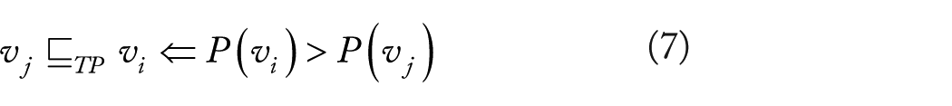
Probability raising. Besides TP, as a second constraint we further require that the arcs are consistent with the condition of PR: this leads to another relation
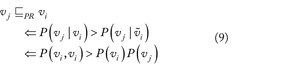
Thus, we model all and only the positive dependant relations. Definition 1 is thus obtained by selecting those PR relations that are consistent with TP

as the core of Suppes’ characterization of causation is relevant. 26
If
Network simplification, regularization, and spurious causality. Suppes’ 26 criteria are known to be necessary but not sufficient to evaluate general causal claims. Even if we restrict to causal cumulative phenomena, the expressivity of probabilistic causality needs to be taken into account.
When dealing with small sample sized data sets (ie, small
We expect all the “statistically relevant” relations to be also prima facie 20 ;
We need to filter out spurious causality instances (a detailed account of these topics, the particular types of spurious structures, and their interpretation for different types of models are available in Ramazzotti and colleagues20,27,30), as we know that prima facie overfits.
A model selection strategy which exploits a regularization schema seems thus the best approach to the task. Practically, this strategy will select simpler (ie, sparse) models according to a penalized likelihood fit criterion—for this reason, it will filter out edges proportionally to how much the regularization is stringent. Also, it will rank spurious association according to a criterion that is consistent with Suppes’ intuition of causality, as likelihood relates to statistical (in)dependence. Alternatives based on likelihood itself, ie, without regularization, do not seem viable to minimize the effect of likelihood’s overfit, that happens unless
Modeling heterogeneous populations
Complex biological processes, eg, proliferation, nutrition, apoptosis, are orchestrated by multiple cooperative networks of proteins and molecules. Therefore, different “mutants” can evade such control mechanisms in different ways. Mutations happen as a random process that is unrelated to the relative fitness advantage that they confer to a cell. As such, different cells will deviate from wild type by exhibiting different mutational signatures during disease progression. This has an implication for many cumulative diseases that arise from populations that are heterogeneous, both at the level of the single patient (intrapatient heterogeneity) and in the population of patients (interpatient heterogeneity). Heterogeneity introduces significant challenges in designing effective treatment strategies, and major efforts are ongoing at deciphering its extent for many diseases such as cancer and HIV.18,20,28
We now introduce a class of mathematical models that are suitable at modeling heterogenous progressions. These models are derived by augmenting BNs with logical formulas and are called monotonic progression networks (MPNs).31,32 The MPNs represent the progression of events that accumulate monotonically (the events accumulate over time and when later events occur earlier events are observed as well) over time, where the conditions for any event to happen is described by a probabilistic version of the canonical boolean operators, ie, conjunction
Following Farahani and Lagergren 31 and Korsunsky et al, 32 we define 1 type of MPNs for each boolean operator: the conjunctive (CMPN), the disjunctive semimonotonic (DMPN), and the exclusive disjunction (XMPN). The operator associated with each network type refers to the logical relation among the parents that eventually lead to the common effect to occur.
Definition 4
Monotonic Progression Networks.31,32 The MPNs are BNs that, for
Definitions for CMPN, DMPN, and XMPN.
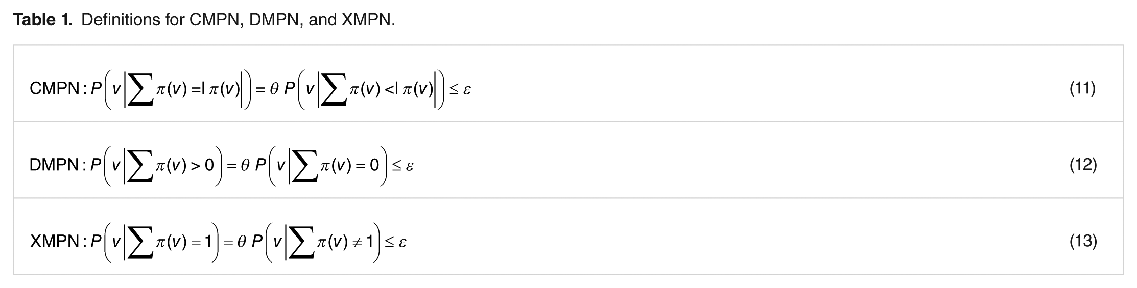
Here,
Model selection with heterogeneous populations. When dealing with heterogeneous populations, the task of model selection, and, more in general, any statistical analysis, are non-trivial. One of the main reasons for this state of affairs is the emergence of statistical paradoxes such as Simpson’s paradox.33,34 This phenomenon refers to the fact that sometimes, associations among dichotomous variables, which are similar within subgroups of a population, eg, women and men, change their statistical trend if the individuals of the subgroups are pooled together. Let us know recall a famous example to this regard. The admissions of the University of Berkeley for the fall of 1973 showed that men applying were much more likely than women to be admitted with a difference that was unlikely to be due to chance. But, when looking at the individual departments separately, it emerged that 6 out of 85 were indead biased in favor of women, whereas only 4 presented a slighly bias against them. The reason for this inconsistency was due to the fact that women tended to apply to competitive departments which had low rates of admissions, whereas men tended to apply to less-competitive departments with high rates of admissions, leading to an apparent bias toward them in the overall population. 35
Similar situations may arise in cancer when different populations of cancer samples are mixed. As an example, let us consider an hypothetical progression leading to the alteration of gene
In the work by Ramazzotti et al, 20 the notion of progression pattern is introduced to describe this situation, defined as a boolean relation among all the genes, members of the parent set of any node as the ones defined by MPNs. To this extent, the authors extend Suppes’ definition of prima facie causality to account for such patterns rather than for relations among atomic events as for Definition 1. Also, they claim that general MPNs can be learned in polynomial time provided that the data set given as input is lifted 20 with a Bernoulli variable per causal relation representing the logical formula involving any parent set.
Following Ramazzotti and colleagues,20,30 we now consider any formula in conjunctive normal form (CNF):

where each
Definition 5
CNF probabilistic causation.20,30 For any CNF formula

Given these premises, we can now define the extended SBCNs, an extension of SBCNs which allows to model heterogeneity as defined probabilistically by MPNs.
Definition 6
Extended SBCN. A BN

Evaluation on Simulated Data
We now evaluate the performance of the inference of SBCN on simulated data, with specific attention on the impact of the constraints based on Suppes’ probabilistic causation on the overall performance. All the simulations are performed with the following settings.
We consider 6 different topological structures: the first 2 where any node has at the most one predecessor, ie, (1) trees, (2) forests, and the others where we set a limit of 3 predecessors and, hence, we consider (3) DAGs with a single source and conjunctive parents, (4) DAGs with multiple sources and conjunctive parents, (5) DAGs with a single source and disjunctive parents, and (6) DAGs with multiple sources and disjunctive parents. For each of these configurations, we generate 100 random structures.
Moreover, we consider 4 different sample sizes (50, 100, 150, and 200 samples) and 9 noise levels (ie, probability of a random entry for the observation of any node in a sample) from 0% to 20% with step 2.5%. Furthermore, we repeat the above settings for networks of 10 and 15 nodes. Any configuration is then sampled 10 times independently, for a total of more than 4 million distinct simulated data sets.
The sequencing quality of mutation profiling for diseases such as cancer and HIV depends on multiple factors such as, but not limited to, depth and coverage of the sequencing. In this work, we introduced errors in the data by means of a random model of noise. A detailed analysis of how more sophisticated models of noise can affect the inference is out of the scope of this study and left for future works.
Finally, the inference of the structure of the SBCN is performed using the algorithm proposed in the work by Ramazzotti et al
20
and the performance is assessed in terms of
In Figures 1 to 3, we show the performance of the inference on simulated data sets of 100 samples and networks of 15 nodes in terms of accurancy, sensitivity, and specificity for different settings which we discuss in detail in the next paragraphs.

Performance of the inference on simulated data sets of 100 samples and networks of 15 nodes in terms of accurancy for the 6 considered topological structures. The y-axis refers to the performance, whereas the x-axis represents the different noise levels.

Performance of the inference on simulated data sets of 100 samples and networks of 15 nodes in terms of sensitivity for the 6 considered topological structures. The y-axis refers to the performance, whereas the x-axis represents the different noise levels.

Performance of the inference on simulated data sets of 100 samples and networks of 15 nodes in terms of specificity for the 6 considered topological structures. The y-axis refers to the performance while the x-axis represents the different noise levels.
Suppes’ prima facie conditions are necessary but not sufficient. We first discuss the performance by applying only the prima facie criteria and we evaluate the obtained prima facie network in terms of accurancy, sensitivity, and specificity on simulated data sets of 100 samples and networks of 15 nodes (see Figures 1 to 3). As expected, the sensitivity is much higher than the specificity implying the significant impact of false positives rather than false negatives for the networks of the prima facie arcs. This result is indeed expected being Suppes’ criteria mostly capable of removing some of the arcs which do not represent valid causal relations rather than assess the exact set of valid arcs. Interestingly, the false negatives are still limited even when we consider DMPN, ie, when we do not have guarantees for the algorithm of Ramazzotti et al 20 to converge. The same simulations with different sample sizes (50, 150, and 200 samples) and on networks of 10 nodes present a similar trend (results not shown here).
The likelihood score overfits the data. In Figures 1 to 3, we also show the performance of the inference by likelihood fit (without any regularizator) on the prima facie network in terms of accurancy, sensitivity, and specificity on simulated data sets of 100 samples and networks of 15 nodes. Once again, in general, sensitivity is much higher than specificity implying also in this case a significant impact of false positives rather than false negatives for the inferred networks. These results make explicit the need for a regularization heuristic when dealing with real (not infinite) sample sized data sets as discussed in the next paragraph. Another interesting consideration comes from the observation that the prima facie networks and the networks inferred via likelihood fit without regularization seem to converge to the same performance as the noise level increases. This is due to the fact that, in general, the prima facie constraints are very conservative in the sense that false positives are admitted as long as false negatives are limited. When the noise level increases, the positive dependencies among nodes are generally reduced and, hence, less arcs pass the prima facie cut for positive dependency. Also in this case, the same simulations with different sample sizes (50, 150, and 200 samples) and on networks of 10 nodes present a similar trend (results not shown here).
Model selection with different regularization strategies. We now investigate the role of different regularizations on the performance. In particular, we consider 2 commonly used regularizations: (1) the Bayesian information criterion (BIC) 36 and (2) the Akaike information criterion (AIC). 37
Although BIC and AIC are both scores based on maximum likelihood estimation and a penalization term to reduce overfitting, yet with distinct approaches, they produce significantly different behaviors. More specifically, BIC assumes the existence of one true statistical model which is generating the data, whereas AIC aims at finding the best approximating model to the unknown data-generating process. As such, BIC may likely underfit, whereas, conversely, AIC might overfit. (Thus, BIC tends to make a trade-off between the likelihood and model complexity with the aim of inferring the statistical model which generates the data. This makes it useful when the purpose is to detect the best model describing the data. Instead, asymptotically, minimizing AIC is equivalent to minimizing the cross validation value. 38 It is this property that makes the AIC score useful in model selection when the purpose is prediction. Overall, the choice of the regularizator tunes the level of sparsity of the retrieved SBCN and, yet, the confidence of the inferred arcs.)
The performance on simulated data sets are shown in Figures 1 to 3. In general, the performance is improved in all the settings with both regularizators, as they succeed in shrinking toward sparse networks.
Furthermore, we observe that the performance obtained by SBCNs is still good even when we consider simulated data generated by DMPN. Although in this case we do not have any guarantee of convergence, in practice, the algorithm seems efficient in approximating the generative model. In conclusion, without any further input, SBCNs can model CMPNs and, yet, depict the more significant arcs of DMPNs. To infer XMPN, the data set needs to be lifted. 20
The same simulations with different sample sizes (50, 150, and 200 samples) and on networks of 10 nodes present a similar trend (results not shown here).
Application to HIV Genetic Data
We now present an example of application of our framework on HIV genomic data. In particular, we study drug resistance in patients under antiretroviral therapy and we select a set of 7 amino acid alterations in the HIV genome to be depicted in the resulting graphical model, namely,
In this study, we consider data sets from the Stanford HIV Drug Resistance Database 39 for 2 protease inhibitors, ritonavir (RTV) and indinavir (IDV). The first data set consists of 179 samples (see Figure 4) and the second of 1035 samples (see Figure 4).
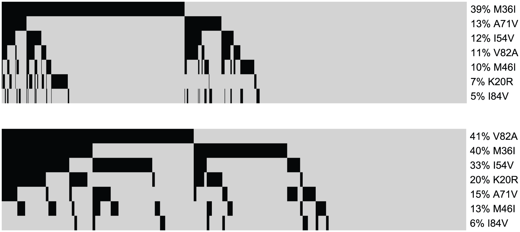
Mutations detected in the genome for 179 patients with HIV under ritonavir (top) and 1035 under indinavir (bottom). Each black rectangle denotes the presence of a mutation in the gene annotated to the right of the plot; percentages correspond to marginal probabilities.
We then infer a model on these data sets by both BN and SBCN. We show the results in Figures 5 where each node represents a mutation and the scores on the arcs measure the confidence in the found relation by nonparametric bootstrap.
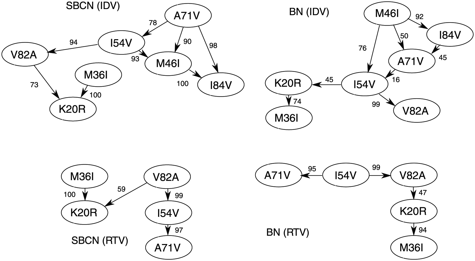
HIV progression of patients under ritonavir or indinavir (Figure 4) described as a Bayesian Network or as a Suppes-Bayes Causal Network. Edges are annotated with nonparametric bootstrap scores.
In this case, it is interesting to observe that the set of dependency relations (ie, any pair of nodes connected by an arc, without considering its direction) depicted both by SBCNs and BNs is very similar, with the main difference being the direction of some connection. This difference is expected and can be attributed to the constrain of TP adopted in the SBCNs. Furthermore, we also observe that most of the found relations in the SBCN are more confident (ie, higher bootstrap score) than the one depicted in the related BN, leading us to observe a higher statistical confidence in the models inferred by SBCNs.
Conclusions
In this work, we investigated the properties of a constrained version of BN, named SBCN, which is particularly sound in modeling the dynamics of system driven by the monotonic accumulation of events, thanks to encoded poset based on Suppes’ theory of probabilistic causation. In particular, we showed how SBCNs can, in general, describe different types of MPN, which makes them capable of characterizing a broad range of cumulative phenomena not limited to cancer evolution and HIV drug resistance.
Besides, we investigated the influence of Suppes’ poset on the inference performance with cross-sectional synthetic data sets. In particular, we showed that Suppes’ constraints are effective in defining a partially order set accounting for accumulating events, with very few false negatives, yet many false positives. To overcome this limitation, we explored the role of 2 maximum likelihood regularization parameters, ie, BIC and AIC, the former being more suitable to test previously conjectured hypotheses and the latter to predict novel hypotheses.
Finally, we showed on a data set of HIV genomic data how SBCN can be effectively adopted to model cumulative phenomena, with results presenting a higher statistical significance compared with standard BNs.
Footnotes
Funding:
The author(s) disclosed receipt of the following financial support for the research, authorship, and/or publication of this article: This work has been partially supported by grants from the SysBioNet project, an MIUR initiative for the Italian Roadmap of European Strategy Forum on Research Infrastructures (ESFRI).
Declaration of conflicting interests:
The author(s) declared no potential conflicts of interest with respect to the research, authorship, and/or publication of this article.
Author Contributions
All authors performed the analysis and wrote the manuscript.