Sage Journals: Discover world-class research

Abstract

Choosing the correct method to predict the incremental effect of a treatment on customer response is critical to optimize targeting policies in many important applications such as churn management and patient care. Two research streams, uplift modeling and heterogeneous treatment effects (HTE), have emerged that scrutinize the incremental effect of a treatment on customer response. So far, these research streams mostly remain independent, with few studies comparing methods across these communities. However, if the goal is to estimate the incremental effect in the best possible way or to make a new contribution in the context of targeting policies, ignoring either uplift modeling or HTE methods is a serious omission. To fill this research gap, the authors benchmark 15 methods from both literatures on synthetic and real-world data sets. They perform benchmarking to contrast the performance of different methods from both research streams and to highlight the importance of evaluating methods from uplift modeling and HTE. The results show that although most methods suffer from volatility, some methods perform better and are more robust than others. In addition, the authors demonstrate that using the incremental effect can substantially improve a targeting policy, but only if academics and practitioners evaluate various methods from both uplift modeling and HTE.

Keywords

customer targeting individual treatment effects uplift modeling heterogeneous treatment effects causal inference benchmarking

Leveraging the incremental effect of a treatment on customer response—hereinafter referred to as the individual treatment effect (ITE)—to optimize targeting policies has been widely discussed in many research areas, including marketing (Ascarza 2018), economics (Athey and Imbens 2016), and data mining (Zhao, Fang, and Simchi-Levi 2017a). In the past few years, several researchers (Devriendt, Moldovan, and Verbeke 2018; Simester, Timoshenko, and Zoumpoulis 2019; Wager and Athey 2018) have written extensively about the incremental effect of a treatment and how to measure, identify, and leverage it. At the same time, practitioners from the industry have emphasized the importance of ITEs (Radcliffe and Surry 2011), companies have increasingly paid attention to the incremental effect of a treatment (e.g., Uber; Chen et al. 2020), and consultancies assess and track ITEs (e.g., Accenture, McKinsey & Company).

The steadily growing literature on ITEs has provided researchers and practitioners with methods and insights that have improved the effectiveness of targeting policies. Two research streams that deal with ITEs have been established: uplift modeling and heterogeneous treatment effects (HTE). Both research streams address similar problems, such as the absence of ground truth and the challenges of estimating the difference between two outcomes that are mutually exclusive. Further, uplift modeling and HTE share a goal: reliably estimating ITEs to optimize targeting policies. Yet, minor differences and the fact that both research streams originate from different communities—HTE from statistics and econometrics, and uplift modeling from marketing, machine learning, and information systems—have led to two almost exclusive research streams (Zhang, Li, and Liu 2021).

Literature integrating and comparing methods from uplift modeling and HTE is sparse (Zhang, Li, and Liu 2021). Gutierrez and Gérardy (2017) were the first to provide a literature review for uplift modeling and HTE methods. The authors discussed the relationship between both research streams and surveyed several methods, mainly from the uplift modeling literature. Ascarza (2018) explicitly recognized the existence of both fields but never compared multiple methods and instead implemented only one approach from the uplift modeling stream. Most recently, Zhang, Li, and Liu (2021) integrated both research streams using a unified language. The authors surveyed and unified multiple methods and discussed the methods’ modeling behavior, usability, interpretability, and scalability. However, to the best of our knowledge, no literature has evaluated and benchmarked methods from uplift modeling and HTE empirically and systematically in a single study. Instead, researchers from both communities have worked independently, comparing their methods only within their particular research stream.

Without comparing methods from uplift modeling and HTE, both communities suffer from redundancies, lose out on opportunities to benefit from each other, miss symbiotic relationships, and fail to contribute to each other. Given the complexity of ITE estimation (Gupta et al. 2020), we must integrate methods and synthesize findings from both research streams. For example, most methods from uplift modeling and HTE suffer from high variance (Devriendt, Moldovan, and Verbeke 2018; Rößler, Tilly, and Schoder 2021; Wager and Athey 2018); combining methods and findings from both streams might lead to more robust solutions. Similarly, if the goal is to estimate ITEs in the best possible way or make a new contribution in the context of targeting policies, ignoring the very rich literature on either uplift modeling or HTE is a serious omission for both academics and practitioners.

Contribution

This article empirically evaluates methods from uplift modeling and HTE. We provide a thorough benchmarking of 15 methods from both research streams on multiple synthetic and real-world data sets. We perform benchmarking to contrast the performance of different methods from uplift modeling and HTE and to highlight the importance of evaluating methods from both research streams. Our study encourages researchers and practitioners to bridge the gap between two related, yet disconnected, research areas. The study also provides a reference point for other academics and practitioners in ITE, uplift modeling, HTE, and targeting policies in general.

Throughout the article, we focus on data with a binary treatment indicator (i.e., customers do or do not receive a treatment) and a binary response variable (e.g., customers do or do not respond). Further, we assume that the data come from randomized controlled experiments (i.e., A/B tests) or satisfy the unconfoundedness assumption and the stable unit treatment value assumption (Athey and Imbens 2015).

The remainder of this article is organized as follows. First, we define both research streams and (formally) demonstrate that both literature branches share an overarching goal. Second, we discuss the relationship between related literature and our research. Third, we present the methodology describing the data sets, the methods evaluated, and the evaluation procedure. Fourth, we demonstrate the results. Finally, we conclude and discuss avenues for future research.

Theoretical Background: Uplift Modeling and Heterogeneous Treatment Effects

Both uplift modeling and HTE are interested in predicting the effect of a treatment that varies across the population (either at the subgroup or individual level) based on observed characteristics—that is, how the likelihood of the population's outcome changes due to a treatment (Athey and Imbens 2016; Kane, Lo, and Zheng 2014). On an individual level, this is called the individual treatment effect (ITE) (Künzel et al. 2019). For example, we might analyze whether a certain marketing promotion (e.g., a discount) prevents a customer from churning.

Predicting the ITE, however, is difficult because of the fundamental problem of causal inference (Holland 1986), which states that for every individual, we observe only one outcome—either the outcome after the individual has been subject to a treatment or the outcome after the individual has not been subject to a treatment, but never both at the same time. Thus, the ITE is not directly observable, and the ground truth is missing.

Uplift modeling and HTE deal with this problem by comparing subgroups or individuals with similar characteristics (i.e., covariates) across the treatment and control groups. This is called the conditional average treatment effect (CATE). To make decisions at an individual level, both uplift modeling and HTE calculate the CATE for the subgroup to which the individual belongs and use this score as an approximation for the ITE (Athey and Imbens 2016). It is important to note that, in most cases, an individual’s ITE will not correspond to the CATE (Künzel et al. 2019). However, researchers argue that the best estimate for the CATE is also the best estimate for the ITE (Künzel et al. 2019).

More formally, both research streams use the same approximation to predict the ITE. For defining the setup, we use Rubin’s (1974) causal model, which compares outcomes we observe and counterfactual outcomes we would have observed under a different treatment. We consider a setup with N individuals, indexed by i = 1, …, N. Let $X_{i}$ be a K-component vector of features or covariates and $T_{i} \in {0, 1}$ a binary treatment indicator, with $T_{i} = 1$ indicating that individual i was subject to a treatment and $T_{i} = 0$ indicating that individual i was not subject to a treatment. For each individual, we denote $Y_{i} (T_{i} = 1) = Y_{i} (1)$ as the outcome of individual i being subject to a treatment, and $Y_{i} (T_{i} = 0) = Y_{i} (0)$ as the outcome of individual i not being subject to a treatment. The ITE, $τ_{i}$ , is defined as the difference in these two outcomes: $τ_{i} = Y_{i} (1) – Y_{i} (0)$ . We will never observe both $Y_{i} (1)$ and $Y_{i} (0)$ because of the fundamental problem of causal inference. Thus, uplift modeling and HTE researchers approximate the ITE by using the following functions, respectively:
$τ_{Uplift} (x) = E [Y_{i} (1) | X_{i} = x] – E [Y_{i} (0) | X_{i} = x],$
(1)
$τ_{HTE} (x) = E [Y_{i} (1) - Y_{i} (0) | X_{i} = x] .$
(2)It follows that $τ_{Uplift} (x) = τ_{HTE} (x)$ . Thus, in this study we simply refer to the approximation as $τ (x)$ . Both uplift modeling and HTE are interested in predicting $\hat{τ} (x)$ .

Related Literature

Our article fits into the growing body of literature that is concerned with optimizing targeting policies using the incremental effect of a treatment on customer response (e.g., Athey, Tibshirani, and Wager 2019; Devriendt, Moldovan, and Verbeke 2018; Gubela et al. 2019; Hitsch and Misra 2018; Simester, Timoshenko, and Zoumpoulis 2019). In contrast, other policies target customers by ignoring the incremental effect and instead concentrate only on customer response (e.g., Coussement, Harrigan, and Benoit 2015). Multiple researchers, however, have shown that targeting policies using the incremental effect can substantially improve profits compared with targeting policies that ignore the incremental effect. (Ascarza 2018; Gubela et al. 2019; Hitsch and Misra 2018). For example, Ascarza (2018) showed that targeting customers based on churn probability (customer response) was counterproductive for a given marketing campaign, recommending instead that customers with the highest sensitivity to the treatment be targeted.

The promising results and the importance of targeting policies in general have led researchers from the uplift modeling and HTE communities to propose various methods to analyze, predict, and measure the incremental effect. Most recently, Zhang, Li, and Liu (2021) unified uplift modeling and HTE, emphasized their connection, and reviewed main applications. Unlike our work, Zhang, Li, and Liu (2021, p. 26) do not focus on benchmarking and instead want “to show how the methods are used in real-world problems.” That is why their comparison is limited with respect to (1) the number of real-world data sets and (2) the number of methods. Further, they do not tune any hyperparameters, use cross-validation, or run any statistical tests. Thus, we complement the work by Zhang, Li, and Liu by providing an extensive and systematic benchmarking.

The Gap in Related Work

Table 1 is an overview of benchmarking studies as well as previous methodological contributions in uplift modeling and HTE. We survey only studies that evaluate at least two methods, use a binary treatment indicator, and assess methods on at least two real-world data sets. Note that we omit two baseline methods: (1) predicting ITEs by calculating the difference between estimations from two independent models, which is often referred to as the two-model approach (TM; Foster, Taylor, and Ruberg 2011; Hansotia and Rukstales 2002), (2) and using the treatment indicator simply as another covariate (Green and Kern 2012; Hill 2011), which is often referred to as the S-learner (SL; Künzel et al. 2019).

Table 1.
Overview of Literature Benchmarking Uplift Modeling and Heterogeneous Treatment Effects Methods.

Studies and Methods Benchmarking Studies

Heterogeneous Treatment Effects Uplift Modeling

Imai and Li (2021) [2] Hitsch and Misra (2018) [2] Künzel et al. (2019) [2] Devriendt, Moldovan, and Verbeke (2018) [4] Gubela et al. (2019) [27] Kane, Lo, and Zheng (2014) [3] Rößler, Tilly, and Schoder (2021) [9] Rzepakowski and Jaroszewciz (2012) [16] Sołtys, Jaroszewicz, and Rzepakowski (2015) [25] Zaniewicz and Jaroszewicz (2017) [28] Zhao, Fang, and Simchi-Levi (2017b) [2]

Heterogeneous Treatment Effects

Hahn, Murray, and Carvalho (2020)[BCF model] X

Athey and Imbens (2015)[Transformed outcome] X

Wager and Athey (2018)[Causal forest] X X

Athey, Tibshirani, and Wager (2019)[GRF] X

Hitsch and Misra (2018)[Treatment effect projection] X

Tian et al. (2014)[Interaction approach] X

Künzel et al. (2019)[XL] X

Nie and Wager (2021)[R-learner] X

Uplift Modeling

Lai (2006)[Lai's method] X X X

Kane, Lo, and Zheng (2014)[LG] X X X

Jaskowski and Jaroszewicz (2012)[Class variable transformation] X X X

Shaar, Abdessalem, and Segard (2016)[Pessimistic uplift] X X

Shaar, Abdessalem, and Segard (2016)[Reflective uplift] X

Sołtys, Jaroszewicz, and Rzepakowski (2015) and Guelman, Guillén, and Pérez-Marín (2015)[U-ED] X X X X

Sołtys, Jaroszewicz, and Rzepakowski (2015)[U-CHI] X

Sołtys, Jaroszewicz, and Rzepakowski (2015)[U-KL] X

Rzepakowski and Jaroszewicz (2012)[Uplift tree] X

Zhao, Fang, and Simchi-Levi (2017b)[CTS] X

Hansotia and Rukstales (2002)[DDP] X

Zaniewicz and Jaroszewicz (2017)[Uplift support vector machine] X

Lo (2002)[TDA] X X X

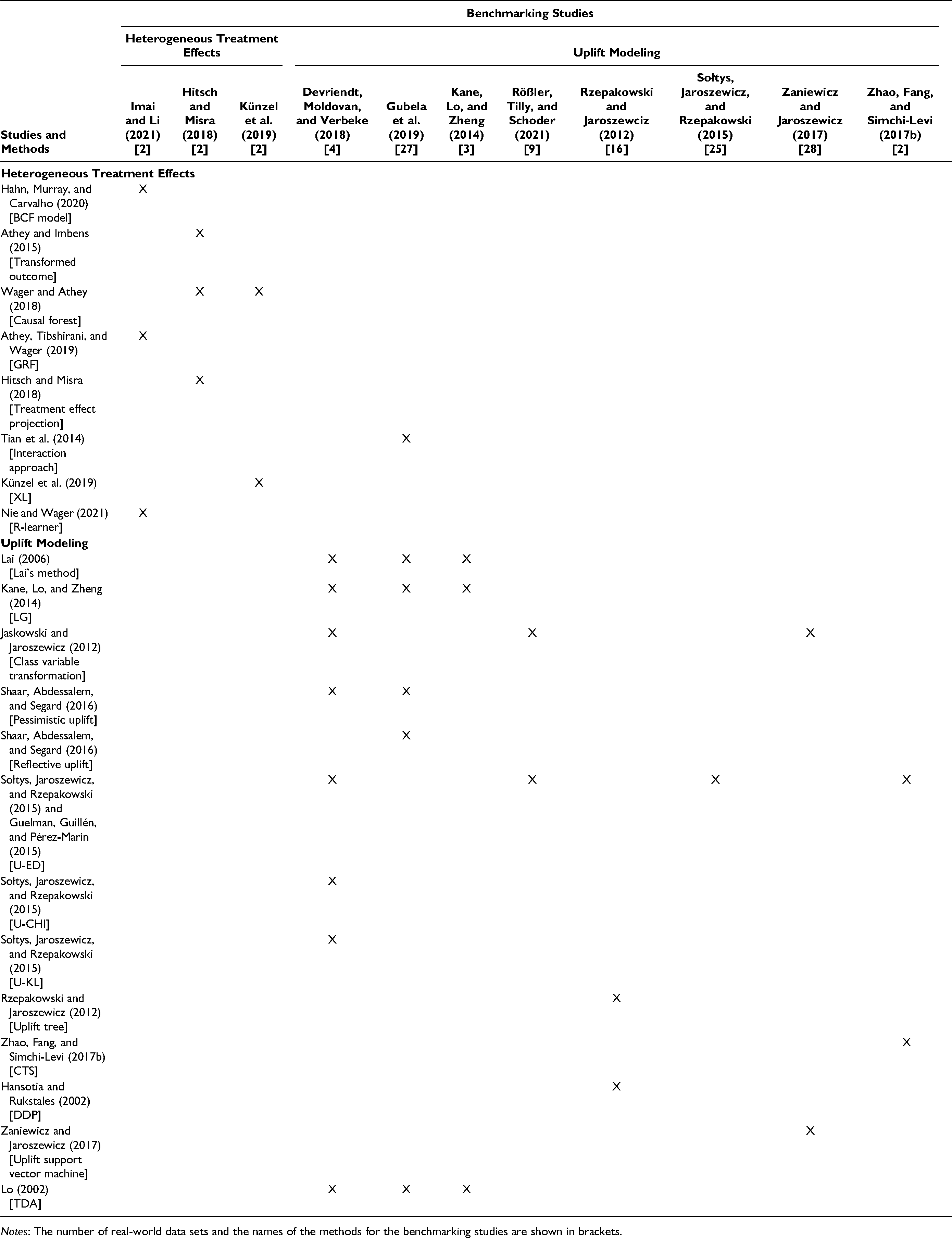
Notes: The number of real-world data sets and the names of the methods for the benchmarking studies are shown in brackets.

Table 1 reveals that researchers from uplift modeling and HTE work independently, with their benchmarking studies in both streams assessing methods only from their own communities. For example, Devriendt, Moldovan, and Verbeke (2018) evaluated ten uplift modeling methods, including Lai's generalization (LG; Kane, Lo, and Zheng 2014), uplift random forest (Sołtys, Jaroszewicz, and Rzepakowski 2015), and treatment dummy approach (TDA; Lo 2002), but not a single method from the HTE stream. Imai and Li (2021) assessed only methods initially proposed in the HTE literature: the Bayesian causal forest (BCF) model (Hahn, Murray, and Carvalho 2020), causal forests (Athey, Tibshirani, and Wager 2019), R-learner (RL; Nie and Wager 2021), and Lasso (Tibshirani 1996). Only Gubela et al. (2019) compared methods from both uplift modeling and HTE. Overall, the authors evaluated the performance of eight methods: one from the HTE literature, that is, the interaction approach (Tian et al. 2014), and seven from the uplift modeling community, such as the TDA (Lo 2002), the class variable transformation (Jaskowski and Jaroszewicz 2012), and LG (Kane, Lo, and Zheng 2014).

Table 1 also illustrates that most uplift modeling and HTE studies compare only a few methods (ignoring baseline methods). Only two studies, Devriendt, Moldovan, and Verbeke (2018) and Gubela et al. (2019), evaluated more than three methods. For example, Zhao, Fang, and Simchi-Levi (2017b) compared their method, contextual treatment selection (CTS), with only uplift random forest (Guelman, Guillén, and Pérez-Marín 2015; Sołtys, Jaroszewicz, and Rzepakowski 2015), ignoring other methods such as the TDA (Lo 2002) and LG (Kane, Lo, and Zheng 2014). Similarly, Imai and Li (2021) did not evaluate methods such as X-learner (XL; Künzel et al. 2019), interaction approach (Tian et al. 2014), or the interaction tree method (IT; Su et al. 2009).

Finally, Table 1 reveals that most benchmarking studies used only a few data sets for the evaluation. We can see that only six studies assessed the performance on more than three data sets (Devriendt, Moldovan, and Verbeke 2018; Gubela et al. 2019; Rößler, Tilly, and Schoder 2021; Rzepakowski and Jaroszewicz 2012; Sołtys, Jaroszewicz, and Rzepakowski 2015; Zaniewicz and Jaroszewicz 2017). Yet, the data sets used by Rzepakowski and Jaroszewicz (2012), Sołtys, Jaroszewicz, and Rzepakowski (2015), and Zaniewicz and Jaroszewicz (2017) had not initially been collected for ITE estimation. The authors used data sets from the University of California, Irvine, repository and artificially created treatment and control groups using one of the covariates as treatment indicator. Further, the 27 data sets used by Gubela et al. (2019, p. 41) all “come from the same provider and exhibit similar features.” Finally, it is striking that studies from the HTE literature considered at most only two real-world data sets when benchmarking ITE methods.

The overarching conclusion emerging from Table 1 is that available methods for ITE prediction have been insufficiently evaluated. Methods were independently assessed only in the respective research stream in which they had been proposed. Further, most studies benchmarked only a few methods and used only a few data sets to evaluate the performance. This motivates a systematic comparison of the performance of ITE methods from uplift modeling and HTE, which, according to Table 1, is missing. We find in the current literature that there are no papers comparing methods from both communities. To close this research gap, we benchmark available ITE methods from uplift modeling and HTE on various synthetic and real-world data sets.

Prior work

Although researchers from both communities have worked independently, it is important to summarize current results with respect to the performance of the algorithms. Next, we elaborate on the findings made by the benchmarking studies from Table 1. Table 2 provides a short description for each method used in this study, including their assumptions and potential strengths and weaknesses. A large part of these methods is based on a nonparametric estimation, that is, on tree-based algorithms (e.g., Hansotia and Rukstales 2002; Sołtys, Jaroszewicz, and Rzepakowski 2015; Wager and Athey 2018). However, we treat these methods as autonomous because they (1) differ on design decisions (e.g., splitting criterion and termination rules) and (2) lead to significantly different results. For a unified survey and a detailed description of all methods in Table 1, we refer to the studies by Zhang, Li, and Liu (2021), Gutierrez and Gérardy (2017), Künzel et al. (2019), and the references therein.

Table 2.
Overview of Methods, Including a Short Description, Their Strengths and Weaknesses, and the Assumptions Made in the Methods.

Study Short Method Description and Potential Strengths and Weaknesses Assumptions

Hansotia and Rukstales (2002) $Δ Δ p$ (DDP): CHAID decision tree (Kass 1980) with a splitting criterion that maximizes the difference of the difference between the treatment and control response probability in the left and right child node (called DDP).Potential weaknesses: Bad performance (Rzepakowski and Jaroszewicz 2012). Binary treatment, binary response randomization^a

e.g., Künzel et al. (2019) Two-model approach (TM): Predict ITEs by calculating the difference between estimations from two independent models. The first model estimates the conditional expectations of the outcomes for individuals subject to a treatment, while the second model estimates the conditional expectations of the outcomes for individuals not subject to a treatment. The ITE is then calculated as the difference between these estimates.Potential strengths: Algorithmic flexibility (Devriendt, Moldovan, and Verbeke 2018); good performance if treatment effect is complicated (Künzel et al. 2019).Potential weaknesses: Bad performance if the treatment effect is simple (Künzel et al. 2019). Randomization^a

e.g., Künzel et al. (2019) S-learner (SL): Predict the response (Y) using all the independent variables and the treatment indicator (T) as covariates (X). Thus, the treatment indicator (T) is simply used as another covariate.Potential strengths: Algorithmic flexibility (Devriendt, Moldovan, and Verbeke 2018).Potential weaknesses: Can be biased toward 0 (Künzel et al. 2019). Randomization^a

Kane, Lo, and Zheng (2014) Lai's generalization (LG): Create a new, transformed outcome variable $Y^{}$ using the response (Y) and treatment indicator (T): $Y^{} = {\begin{matrix} 0 if T = 0 and Y = 1 \\ 1 if T = 0 and Y = 0 \\ 2 if T = 1 and Y = 1 \\ 3 if T = 1 and Y = 0 \end{matrix} .$ Then approximate the ITE by weighting the outcome probabilities with the given treatment–control ratio: $\hat{τ} (x) = E [\frac{P (Y^{} = 2)}{P (T = 1)} + \frac{P (Y^{} = 1)}{P (T = 0)} - \frac{P (Y^{} = 3)}{P (T = 1)} - \frac{P (Y^{} = 4)}{P (T = 0)} | X_{i} = x] .$ Potential strengths: Bias correction of imbalanced treatment–control ratio (Kane, Lo, and Zheng 2014); algorithmic flexibility (e.g., Devriendt, Moldovan, and Verbeke 2018).Potential weaknesses: Volatile performance (Devriendt, Moldovan, and Verbeke 2018; Gubela et al. 2019) Binary treatment, binary response randomization^a

Künzel et al. (2019) X-learner (XL): First, the method models Y_i(1) and Y_i(0) separately using the treatment and control groups, respectively. Second, it imputes the treatment effect for each individual—that is, the difference between the true outcome and the estimated outcome using the control estimator is calculated for the individuals in the treatment group; for the individuals in the control group, the difference between the estimated outcome using the treatment estimator and the true outcome is calculated. The imputed treatment effects D¹ and D⁰ are then used as outcome variables to estimate ${\hat{τ}}_{1} (x) = E [D^{1} | X = x]$ and ${\hat{τ}}_{0} (x) = E [D^{0} | X = x]$ using any type of base learner (e.g., decision tree, regression model). Third, the ITE is predicted by weighting the estimates from the second step with a weight function $g \in [0, 1]$ : $\hat{τ} (x) = g (x) {\hat{τ}}_{0} (x) + [1 – g (x)] {\hat{τ}}_{1} (x)$ .Potential strengths: Can adapt to structural properties (e.g., sparsity) (Künzel et al. 2019); good performance when one of the treatment groups is much larger than the other (Künzel et al. 2019); algorithmic flexibility (Künzel et al. 2019). Binary treatment, randomization^a

Lo (2002) Treatment dummy approach (TDA): Use covariates (X), treatment indicator (T), and the interaction between covariates and treatment indicator (X × T) as independent variables and the response variable (Y) as dependent variable in a logistic regression to estimate the ITE.Potential strengths: Good performance (Devriendt, Moldovan, and Verbeke 2018; Gubela et al. 2019).Potential weaknesses: Large compound errors and multicollinearity (Devriendt, Moldovan, and Verbeke 2018). Binary treatment, randomization^a

Nie and Wager (2021) R-learner (RL): Decompose the CATE function such that it depends on the conditional mean outcome and the treatment propensity. Subsequently, first estimate the conditional mean outcome and the treatment propensity and then estimate the ITE by minimizing the objective function (called R-loss).Potential strengths: Algorithmic flexibility (Nie and Wager 2021).Potential weaknesses: Volatile performance (Imai and Li 2021; Nie and Wager 2021). Randomization^a

Sołtys, Jaroszewicz, and Rzepakowski (2015) and Guelman, Guillén, and Pérez-Marín (2015) Uplift random forest: Bagging of CART (Breiman et al. 1984) decision trees with Kullback–Leibler divergence, chi-squared divergence, or squared Euclidean distance as splitting criterion.Potential strengths: Good performance (Devriendt, Moldovan, and Verbeke 2018; Rzepakowski and Jaroszewicz 2012; Sołtys, Jaroszewicz, and Rzepakowski 2015).Potential weaknesses: Volatile performance (Rößler, Tilly, and Schoder 2021). Randomization^a

Zhao, Fang, and Simchi-Levi (2017b) Contextual treatment selection (CTS): Random forest with expected response as splitting criterion, which directly optimizes the uplift performance.Potential strengths: Good performance (Zhao, Fang, and Simchi-Levi 2017b). Randomization^a

Su et al. (2009) Interaction tree (IT): CART decision tree (Breiman et al. 1984) with G-statistic as splitting criterion, which automatically finds subgroups in which the treatment effect is found prominent as well as subgroups in which the treatment has a negligible or negative effect.Potential weakness: Does not place value on splits that improve the fit (Athey and Imbens 2016). Binary treatment, randomization^a

Su et al. (2012) Causal inference tree (CIT): CART decision tree (Breiman et al. 1984) with likelihood ratio test statistic as splitting criterion, which automatically finds subgroups in which the propensity and treatment effect become more homogeneous. Binary treatment, randomization^a

Athey, Tibshirani, and Wager (2019) Generalized random forest (GRF): Family of nonparametric estimators that inherit the properties of random forests (Breiman et al. 1984). The estimators can be used for a wide range of statistical settings. When used for heterogeneous treatment effect estimation, the method is very similar to the causal forest method (Wager and Athey 2018). The splitting criterion optimizes splits associated with treatment effect heterogeneity by maximizing the negative expected mean squared error. Further, the authors use different samples for partitioning the covariate space and estimating the CATE scores. Before growing a tree, they split the training sample into an estimation samples, which is used only for CATE score estimation, and a training sample that is used only for selecting tree splits.Potential strengths: Good performance (Athey and Imbens 2016; Hitsch and Misra 2018; Imai and Li 2021; Wager and Athey 2018). Binary treatment, randomization^a

Hahn, Murray, and Carvalho (2020) Bayesian causal forest (BCF) model: Decompose the CATE function such that it depends on the prognostic effect (i.e., effect of covariates excluding the treatment variable on outcome) and on the treatment effect. The authors then model the prognostic effect and the treatment effect independently using Bayesian additive regression tree priors.Potential strengths: Good performance (Hahn, Murray, and Carvalho 2020; Imai and Li 2021). Binary treatment, randomization^a

^a
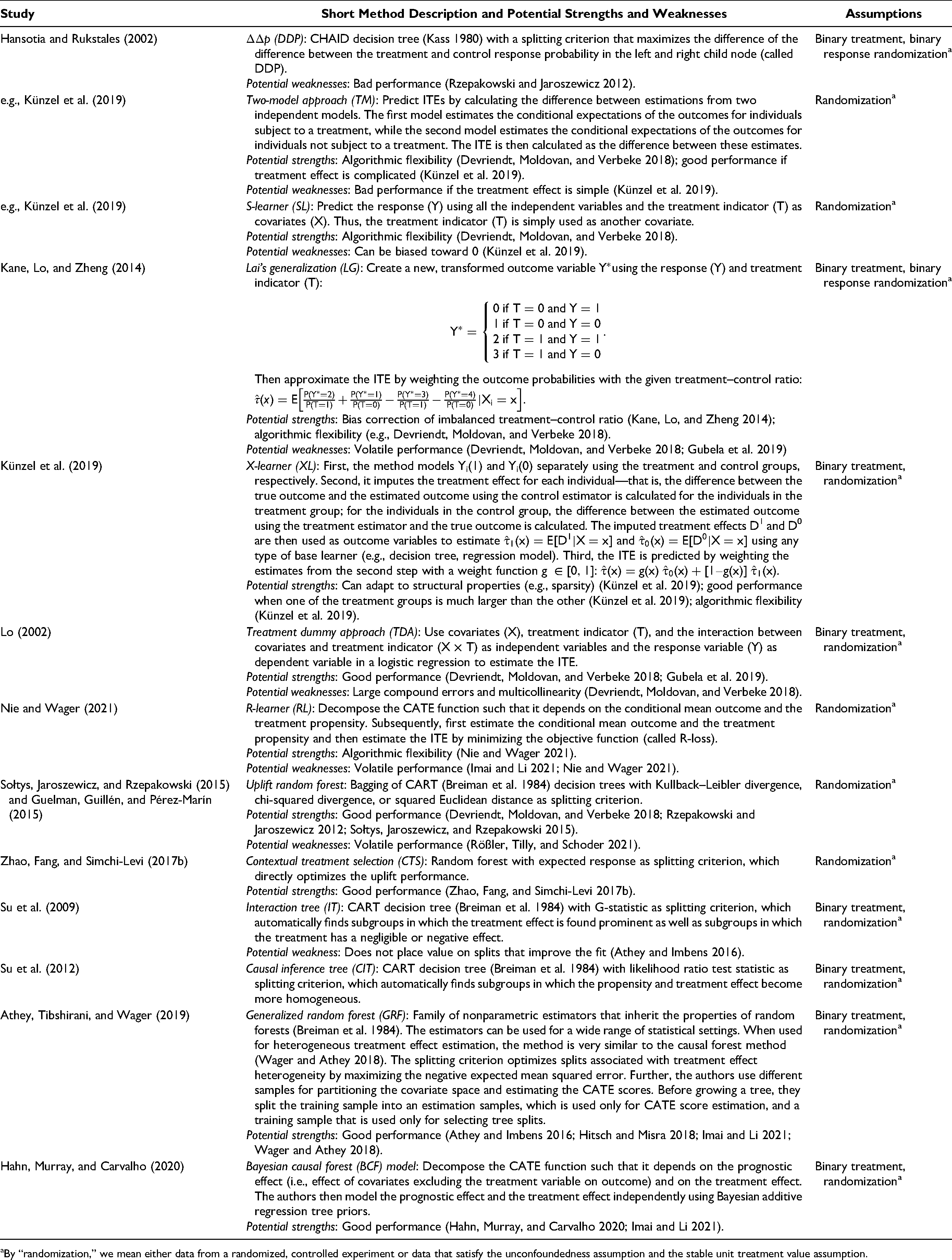
By “randomization,” we mean either data from a randomized, controlled experiment or data that satisfy the unconfoundedness assumption and the stable unit treatment value assumption.

The BCF model (Hahn, Murray, and Carvalho 2020) was evaluated in only one study (Imai and Li 2021). The authors found that the method did not perform significantly better than random targeting. Introducing budget constraints (i.e., treating a maximum of 20% of the customers), they observed that the BCF model improved on not only random targeting but also other methods, including Lasso (Tibshirani 1996) and RL (Nie and Wager 2021).

Imai and Li (2021) found that the generalized random forest (GRF; Athey, Tibshirani, and Wager 2019) did not outperform random targeting. After introducing the aforementioned budget constraint, however, the authors found that the GRF significantly outperforms random targeting and other methods. Further, they showed that the GRF was the most stable method with the smallest standard errors. Although the causal forest (Wager and Athey 2018)—a special case of the GRF—performed very well in one study (Hitsch and Misra 2018), Künzel et al. (2019) showed that their method, the XL, outperformed the causal forest.

Most of the benchmarking studies showed that the methods of Athey and Imbens (2015) and Jaskowski and Jaroszewicz (2012) were consistently among the worst-performing algorithms. For example, Devriendt, Moldovan, and Verbeke (2018) demonstrated that the approach by Jaskowski and Jaroszewicz (2012) performed worst. Other studies found similar results (Gubela et al. 2019; Rößler, Tilly, and Schoder 2021). The same is true for the transformed outcome approach of Athey and Imbens (2015) (Hitsch and Misra 2018).

RL (Nie and Wager 2021) and XL (Künzel et al. 2019) were each evaluated only once by the benchmarking studies. While Imai and Li (2021) demonstrated that the RL did not outperform random targeting, Künzel et al. (2019) showed that the XL leads to promising results, especially when one of treatment group is much larger than the other.

Lai's (2006) method and its successor, Lai's generalization (LG; Kane, Lo, and Zheng 2014), were evaluated by various authors (Devriendt, Moldovan, and Verbeke 2018; Gubela et al. 2019; Kane, Lo, and Zheng 2014). Whereas Kane, Lo, and Zheng (2014) argued that Lai's method performs worse than LG, Gubela et al. (2019) found that LG performs no better than Lai's method. Devriendt, Moldovan, and Verbeke (2018) showed that both methods performed well compared with other methods (e.g., transformed outcome [Jaskowski and Jaroszewicz 2012] and pessimistic uplift modeling [Shaar et al. 2016])

The uplift random forest (Guelman, Guillén, and Pérez-Marín 2015; Sołtys, Jaroszewicz, and Rzepakowski 2015) was consistently among the best-performing approaches in most benchmarking studies (Devriendt, Moldovan, and Verbeke 2018; Rößler, Tilly, and Schoder 2021; Sołtys, Jaroszewicz, and Rzepakowski 2015). Further, several authors (see, e.g., Guelman, Guillén, and Pérez-Marín 2015; Sołtys, Jaroszewicz, and Rzepakowski 2015) demonstrated that the uplift random forest outperformed tree-based uplift algorithms such as the uplift tree (Rzepakowski and Jaroszewicz 2012) and the $Δ Δ p$ (DDP) tree (Hansotia and Rukstales 2002). However, Rößler, Tilly, and Schoder (2021) found that the uplift random forest suffered from volatility, and Zhao, Fang, and Simchi-Levi (2017b) showed that the performance of CTS can be superior to that of the uplift random forest.

The TDA (Lo 2002) has performed well in most benchmarking studies (Devriendt, Moldovan, and Verbeke 2018; Gubela et al. 2019). Gubela et al. (2019) found that the TDA showed the most promising results when combined with any base learner. In contrast, they argued that the method proposed by Tian et al. (2014), which is very similar to the TDA, was inferior to the latter.

Overall, as other researchers have already noted (Devriendt, Moldovan, and Verbeke 2018; Rößler, Tilly, and Schoder 2021), the algorithms’ performances vary from study to study. While most researchers agree on the weak performance of transformed outcome and class variable transformation, researchers disagree on the performance of other algorithms, such as tree-based ensembles like the causal forest and the uplift random forest. Other algorithms—XL, the BCF model, the causal inference tree (CIT), and RL—have been insufficiently evaluated. Again, this motivates a systematic comparison of the performance of various ITE methods. We shed light on the performance of various algorithms by benchmarking available methods on various synthetic and real-world data sets.

Methodology

This section describes the setup that compares 15 methods across both research streams on 27 synthetic and 6 real-world data sets. In the following, we describe the data sets and methods used as well as the evaluation procedure.

Data Sets

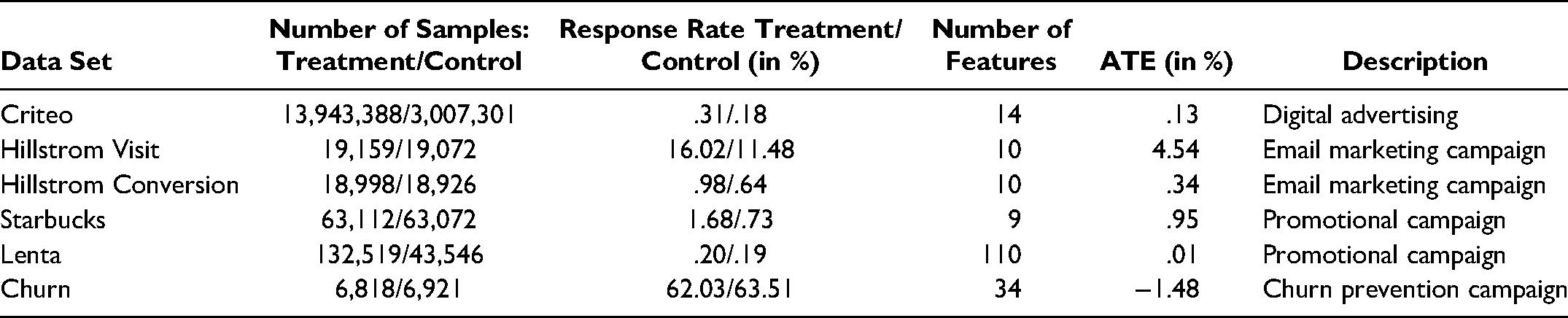
We performed a benchmark on 27 synthetic and 6 real-world data sets. The setup was designed to consider different data set characteristics, such as varying sizes and varying response rates. Table 3 summarizes the real-world data sets in terms of the number of samples and response rates in the treatment and control groups, number of features, and average treatment effect (ATE).

Table 3.
Summary of Real-World Data Sets.

Data Set Number of Samples: Treatment/Control Response Rate Treatment/ Control (in %) Number of Features ATE (in %) Description

Criteo 13,943,388/3,007,301 .31/.18 14 .13 Digital advertising

Hillstrom Visit 19,159/19,072 16.02/11.48 10 4.54 Email marketing campaign

Hillstrom Conversion 18,998/18,926 .98/.64 10 .34 Email marketing campaign

Starbucks 63,112/63,072 1.68/.73 9 .95 Promotional campaign

Lenta 132,519/43,546 .20/.19 110 .01 Promotional campaign

Churn 6,818/6,921 62.03/63.51 34 −1.48 Churn prevention campaign

Synthetic

The synthetic data sets were motivated by Wager and Athey (2018) and Künzel et al. (2019). We created 50.000 samples with a 20-dimensional feature vector $X_{i} \sim N (0, Σ),$ where Σ is a symmetric, positive-semidefinite covariance matrix with covariance = .3 The outcome was then simulated using an indicator function:
$Y_{i} (X_{i,} T_{i}) = {\begin{matrix} 1 if Γ_{i} (X_{i}, T_{i}) > ρ \\ 0 if Γ_{i} (X_{i}, T_{i}) \leq ρ \end{matrix},$
(3)where $ρ$ is a threshold and $Γ_{i} (X_{i}, T_{i})$ is the potential outcome: $Γ_{i} (X_{i}, T_{i}) = μ_{T_{i}} (X_{i}) + σ ε_{i}$ with $ε_{i} \sim N (0, 1)$ independent of $X_{i};$ $μ_{1} (X_{i}) = \frac{1}{2} ζ (x_{1}) ζ (x_{2})$ and $μ_{0} (X_{i}) = – \frac{1}{2} ζ (x_{1}) ζ (x_{2}),$ with
$ζ (x) = \frac{2}{1 + e^{– 12 (x – \frac{1}{2})}},$
(4)as a complex nonlinear function. Finally, the treatment indicator was created according to $T_{i} \sim Bernoulli [e^{} (X_{i})]$ . We simulated various data sets with varying error terms $σ \in {.5, 1 .0, 2 .0}$ , propensity scores $e^{} (X_{i}) \in {.2, .5, .8}$ , and percentile thresholds $ρ \in {20 th, 50 th, 80 th}$ based on $Γ_{i} (X_{i}, T_{i})$ , creating a total of 27 synthetic data sets.

Criteo

The Criteo data set, which comes from a randomized control trial conducted in the digital advertising industry, was made available by Diemert et al. (2018). After we removed duplicates, the data set contained around 17 million observations and 14 different features. The treatment–control ratio was around 5:1, with 13,943,388 samples in the treatment group and 3,007,301 samples in the control group. The response rates in the treatment and control groups were very low, at .31% and .18%, respectively, and thus, the ATE was .13%.

Hillstrom

The Hillstrom data set comes from an email marketing campaign from MineThatData (Hillstrom 2008). It comprises 42,693 customers: 21,387 in the treatment group and 21,306 in the control group. Overall, the data set contains ten covariates and three target variables: visit (yes/no), purchase (yes/no), and conversion (numerical). We created two data sets from the Hillstrom data set: one with visit as target variable (Hillstrom Visit) and another with conversion as target variable, where a conversion > 0 was considered a positive response (Hillstrom Conversion). After we removed duplicates in the former data set, 19,159 customers were in the treatment group and 19,072 in the control group. The response rates in the treatment and control group were higher than those in the Criteo data set: 16.02% and 11.48%, respectively. Thus, the ATE was 4.54%. In Hillstrom Conversion, the response rates were low, with a .98% response in the treatment group and .64% in the control group. Thus, the ATE was .34%. Again, we dropped duplicates, leaving 18,998 customers in the treatment group and 18,926 in the control group. In line with previous studies (Devriendt, Moldovan, and Verbeke 2018; Kane, Lo, and Zheng 2014), we considered only the promotion of women's merchandise.

Starbucks

The Starbucks data set,¹ which comes from a Starbucks promotional campaign conducted via a reward mobile app, contains 126,184 observations and nine different features. Although the treatment–control ratio is 1:1, with 63,112 samples in the treatment group and 63,072 samples in the control group, the response rates in both groups are low: 1.68% in the treatment group and .73% in the control group, resulting in an ATE of .95%.

Lenta

The Lenta data set came from one of the largest Russian wholesalers and was released as part of a hackathon in collaboration with Microsoft (https://bigtarget.online). It relates to an SMS targeting campaign to increase the likelihood of customers buying products in physical stores. After we removed variables with too many missing values, the data set contained 110 features. Further, we dropped rows with any missing values, resulting in 176,065 samples: 132,519 samples in the treatment group and 43,546 samples in the control group. The response rates were .2% and .19% in the treatment and control groups, respectively, and thus the ATE was .01%.

Churn

The final data set comprises private data from a company in Germany with fixed-term contracts and autorenewal, which we refer to as the Churn data set.² Over one year, the firm ran several churn prevention campaigns to investigate whether a discount offer for the next contract period would prevent customers from churning. In each trial, customers were selected whose contracts had not yet been canceled but who had the same contractual end date. These customers were divided randomly and equally into a control and treatment group. All customers in the treatment group were subject to the same treatment: a discount for the next contract period. The costs for each treatment, including expenses for sending the offer via mail and the discount itself, were $40. Customers in the control group received no incentive. After the cancellation date, the company tracked who renewed and who canceled the contract. The data set comprises 13,739 customers: 6,818 in the treatment group and 6,921 in the control group. In contrast to the Criteo and Starbucks data sets, the response rates (i.e., retention rate) in the Churn data set are much higher, with a 62.03% response in the treatment group and a 63.51% response in the control group. The ATE is negative at −1.48% because the response rate in the control group is marginally higher than the response rate in the treatment group. Overall, the company collected 34 features, including continuous and categorical features covering sociodemographic information, campaign details, and consumer behavior data. The company did not obtain customer relationship information such as a customer life cycle value.

Methods

In our setup, we compared 15 methods from both research streams. Table 4 provides a full overview of the various methods evaluated in this study, including base learner, abbreviation, research stream, and references to where the method was proposed.

Table 4.
Overview of the Methods Used in the Methodology.

Method Base Learner Abbreviation Research Stream Reference

Two-model approach Random forest TM Uplift modeling/HTE (baseline) e.g., Künzel et al. (2019)

X-learner Random forest XL HTE Künzel et al. (2019)

Lai's generalization Random forest LG Uplift modeling Kane, Lo, and Zheng (2014)

Uplift random forest with squared Euclidean distance Random forest U-ED Uplift modeling Sołtys, Jaroszewicz, and Rzepakowski (2015) and Guelman, Guillén, and Pérez-Marín (2015)

Uplift random forest with Kullback–Leibler divergence Random forest U-KL Uplift modeling Sołtys, Jaroszewicz, and Rzepakowski (2015)

Uplift random forest with chi-squared divergence Random forest U-CHI Uplift modeling Sołtys, Jaroszewicz, and Rzepakowski (2015)

Random forest with ΔΔp criterion Random forest DDP Uplift modeling Hansotia and Rukstales (2002)

Contextual treatment selection Random forest CTS Uplift modeling Zhao et al. (2017a)

Random forest with interaction tree criterion Random forest IT HTE Su et al. (2009)

Random forest with causal inference criterion Random forest CIT HTE Su et al. (2012)

S-learner Random forest SL Uplift modeling/HTE (baseline) e.g., Künzel et al. (2019)

Treatment dummy approach Logistic regression TDA Uplift modeling Lo (2002)

R-learner Random forest RL HTE Nie and Wager (2021)

BCF Bayesian additive regression trees BCF HTE Hahn, Murray, and Carvalho (2020)

GRF Random forest GRF HTE Athey, Tibshirani, and Wager (2019)

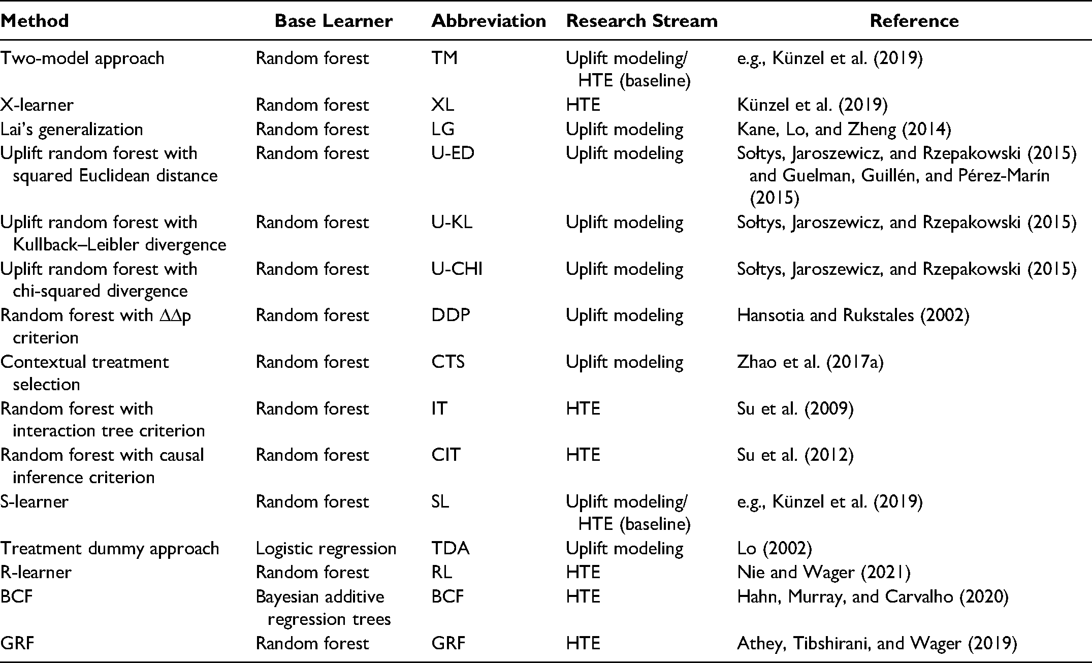
Table 4 illustrates that we evaluated seven methods from uplift modeling, six methods from HTE, and two baseline methods commonly used in both research streams. With the exception of TDA and BCF, each method was based on the random forest because Gubela et al. (2019) found that most algorithms perform well with random forest as base learner. In addition, this enables us to have the same baseline for comparison. Note that the IT (Su et al. 2009) and the CIT (Su et al. 2012) were initially proposed in the form of a classification and regression tree (CART; Breiman et al. 1984) and that the DDP criterion was initially suggested as a split criterion in a chi-square automatic interaction detection (CHAID) decision tree (Kass 1980). However, we used the split criteria proposed in all three studies in a random forest because ensembles have been shown to perform much better than single decision trees (Sołtys, Jaroszewicz, and Rzepakowski 2015).

For each method based on the random forest, we applied hyperparameter tuning for three parameters and for each data set to avoid overfitting: n_estimators, max_depth, and min_samples_leaf. More information about training and hyperparameter tuning can be found in the following subsection and Appendix A.

We implemented TM, LG, TDA, and SL using scikit-learn (Pedregosa et al. 2011), GRF using EconML (https://github.com/microsoft/EconML), and BCF using the Accelerated Bayesian Causal Forests³ package; the remaining methods were implemented using CausalML (Chen et al. 2020). The full code of the benchmarking can be accessed via GitHub to enable other researchers to replicate or even extend our results.⁴

Evaluation Metrics

We split the real-world and synthetic data sets into 80% training and 20% testing while stratifying the treatment and response variable. We used the training samples and tenfold cross-validation for the Hillstrom Visit, Hillstrom Conversion, Starbucks, Lenta, and Churn data sets to select the best hyperparameters for each method, again using stratification with the treatment and response variable. We omitted cross-validation for the Criteo data set, as its size was much larger than the other data sets, and instead split the training samples into 80% training and 20% validation using stratification. We also used tenfold cross-validation for the synthetic data sets, but we omitted hyperparameter tuning and instead fixed the values. Predictions and Qini-related metrics (i.e., the deciles of the Qini curve and the unscaled Qini coefficient) were computed for each method, data set, and validation fold. We then chose the best hyperparameter settings based on the (average) unscaled Qini coefficient on the validation fold(s).

Typically, the performance of predictive algorithms is compared in terms of actual versus predicted outcomes. However, because of the fundamental problem of causal inference (see the “Theoretical Background” section), we do not observe the actual values. Consequently, most researchers use a decile-based evaluation metric to evaluate the performance of a predictive model (Gubela et al. 2019). The Qini curve and the unscaled Qini coefficient are metrics commonly used by researchers and practitioners (Devriendt, Moldovan, and Verbeke 2018; Gubela et al. 2019; Imai and Li 2021; Rößler, Tilly, and Schoder 2021) and assess the performance by comparing groups of customers rather than individual customers. Inspired by the Gini curve, the Qini curve plots the cumulative difference in response rate between treatment and control samples as a function of the number of targeted samples ranked by the method from high to low (Devriendt, Moldovan, and Verbeke 2018). To be more specific, in each quantile (often decile), we compare the customers with the k% highest scores of the treatment group with the k% highest scores of the control group and estimate the difference in response rates between the two. This difference is called “uplift.” Thus, the higher the response rate in the treatment group compared with the response rate in the control group, the higher the uplift value for a quantile. The uplift value targeting everyone (i.e., in the last quantile) equals the ATE. The optimal Qini curve ranks treatment responder ahead of treatment nonresponder in the treatment group and control nonresponder ahead of control responder in the control group. Ideally, the Qini curve of an algorithm should achieve high and increasing uplift values in the first quantiles (e.g., 50% uplift in 10% decile, 60% uplift in 20% decile) until the uplift saddles and eventually begins to decrease until it is equal to the ATE (i.e., the uplift value when targeting all customers). The unscaled Qini coefficient serves as a single number metric. It is defined as the ratio of the area under the actual Qini curve to the area under the diagonal—corresponding to random targeting (Radcliffe and Surry 2011). If the value is greater than one, the actual model is better than random targeting. In general, the higher the value, the better the uplift modeling method.

Finally, we compared and evaluated the models based on the (average) performance on the test set. That is, we used the ten models from cross-validation with the best hyperparameter settings, estimated their scores on the independent test sample, and calculated the (average) Qini curves and (average) unscaled Qini coefficients as well as the standard deviation of the average unscaled Qini coefficients. Note that for the Criteo data set, we had only one model, as we omitted cross-validation; thus, we could not calculate any standard deviations.

Statistical Tests

To detect significant differences in performances and robustness, we validated the results of the benchmarking, more specifically on the test folds, using a statistical comparison. As proposed by Demšar (2006), we performed a nonparametric Friedman (1940) test followed by a corresponding post hoc test. First, for each algorithm $j \in J = {j_{1}, \dots, j_{15}}$ , we calculated the rank $r_{i}^{j}$ on the i^th data set. In case of ties, average ranks were assigned. Second, we calculated the average ranking ${\bar{r}}_{j}$ for the j method over the data sets. Finally, we calculated the test statistic, which is distributed to the F-distribution with k − 1 and $(k - 1) (N - 1)$ degrees of freedom as follows:
$F_{F} = \frac{(N - 1) χ_{F}^{2}}{N (k - 1) - χ_{F}^{2}},$
(5)where $χ_{F}^{2}$ is defined as
$χ_{F}^{2} = \frac{12 N}{k (k + 1)} [{(\frac{1}{N} \sum_{i} r_{i}^{j})}^{2} - \frac{k {(k + 1)}^{2}}{4}] .$
(6)At a level of $α = .05$ , we are interested in rejecting the null hypothesis stating that all algorithms are equivalent. If we reject the null hypothesis, a post hoc Nemenyi (1963) test compares all of the methods to each other.

Results

The results consist of the performance estimates of 15 methods on 27 synthetic and 6 real-world data sets. The performance is evaluated first in terms of the unscaled Qini coefficient and then in terms of the Qini curve. While the first measure helps contrast the performance of various methods, the second describes strategies for improving the targeting policy through the application of an ITE method.

Unscaled Qini Coefficient

Table 5 summarizes the (average) unscaled Qini coefficients on the test fold(s) and their standard deviations for all methods, real-world data sets, and aggregated synthetic data sets. Overall, we observe that none of the methods evaluated in this study outperforms the others on all data sets. With respect to the synthetic data sets in particular, we found that all methods, except TDA, performed well. We could not derive any boundary conditions using the synthetic data sets—that is, we could not indicate which method performed best under which data set characteristics. We only found that the RL's performance was worse than the performance of the other methods on some synthetic data sets, but we could not identify any patterns. Next, we elaborate that some of the methods perform better/worse in terms of the (average) unscaled Qini coefficient and that some are more robust/volatile in terms of the (average) unscaled Qini coefficients’ standard deviation, interquartile range, and difference between maximum and minimum values.

Table 5.
(Average) Unscaled Qini Coefficients on the Test Fold(s) for All Methods on the Real-World and Synthetic Data Sets.

Method Synthetic Criteo Hillstrom Visit Hillstrom Conversion Starbucks Lenta Churn

RL 1.7388 (.01) .9462 1.0599 (.05) 1.0022 (.24) 1.1646 (.04) 1.1178 (.35) 1.5227 (.47)

SL 1.7985 (.00) 1.4846 .9526 (.05) 1.9497 (.23) 1.3520 (.06) 1.2160 (.20) 2.1526 (.89)

TM 1.7932 (.01) 1.4846 .9296 (.06) 2.0011 (.23) 1.3577 (.03) 1.1824 (.36) 2.1127 (.33)

LG 1.7758 (.00) 1.1462 .9584 (.05) .7838 (.14) 1.0421 (.03) 2.0986 (.07) 1.4193 (.31)

CTS 1.7747 (.00) 1.2538 1.3766 (.04) 1.1665 (.21) 1.4598 (.03) 1.3254 (.25) 1.3576 (.39)

U-CHI 1.8009 (.00) 1.6077 1.2999 (.03) 1.1059 (.14) 1.4188 (.03) 1.4206 (.23) 1.6838 (.18)

DDP 1.7956 (.00) 1.5769 1.2730 (.03) 1.2292 (.21) 1.4038 (.03) 1.1836 (.18) 1.4766 (.32)

U-ED 1.8028 (.00) 1.5154 1.3001 (.03) 1.1481 (.20) 1.4461 (.02) 1.0838 (.25) 1.5718 (.33)

IT 1.8042 (.01) 1.5615 1.3011 (.03) 1.2054 (.18) 1.3893 (.02) 1.1762 (.20) 1.3519 (.38)

GRF 1.8030 (.01) 1.6077 1.3659 (.03) 1.3719 (.24) 1.5516 (.03) .8862 (.18) .8761 (.47)

BCF 1.7998 (.00) 1.4385 1.3686 (.02) 1.7168 (.28) 1.6097 (.02) 1.1356 (.12) .9788 (.51)

CIT 1.8080 (.00) 1.6077 1.3720 (.03) 1.3643 (.25) 1.4632 (.03) 1.0836 (.28) 1.9068 (.29)

U-KL 1.8003 (.00) 1.7154 1.2979 (.03) 1.0589 (.21) 1.4137 (.03) 1.2794 (.23) 1.4768 (.27)

XL 1.7958 (.01) 1.4846 1.0492 (.04) 1.3681 (.16) 1.3587 (.02) .8478 (.32) 1.6484 (.27)

TDA 1.1856 (.00) 1.7923 .9265 (.07) .5832 (.09) .5472 (.01) .2216 (.17) 1.0639 (2.07)

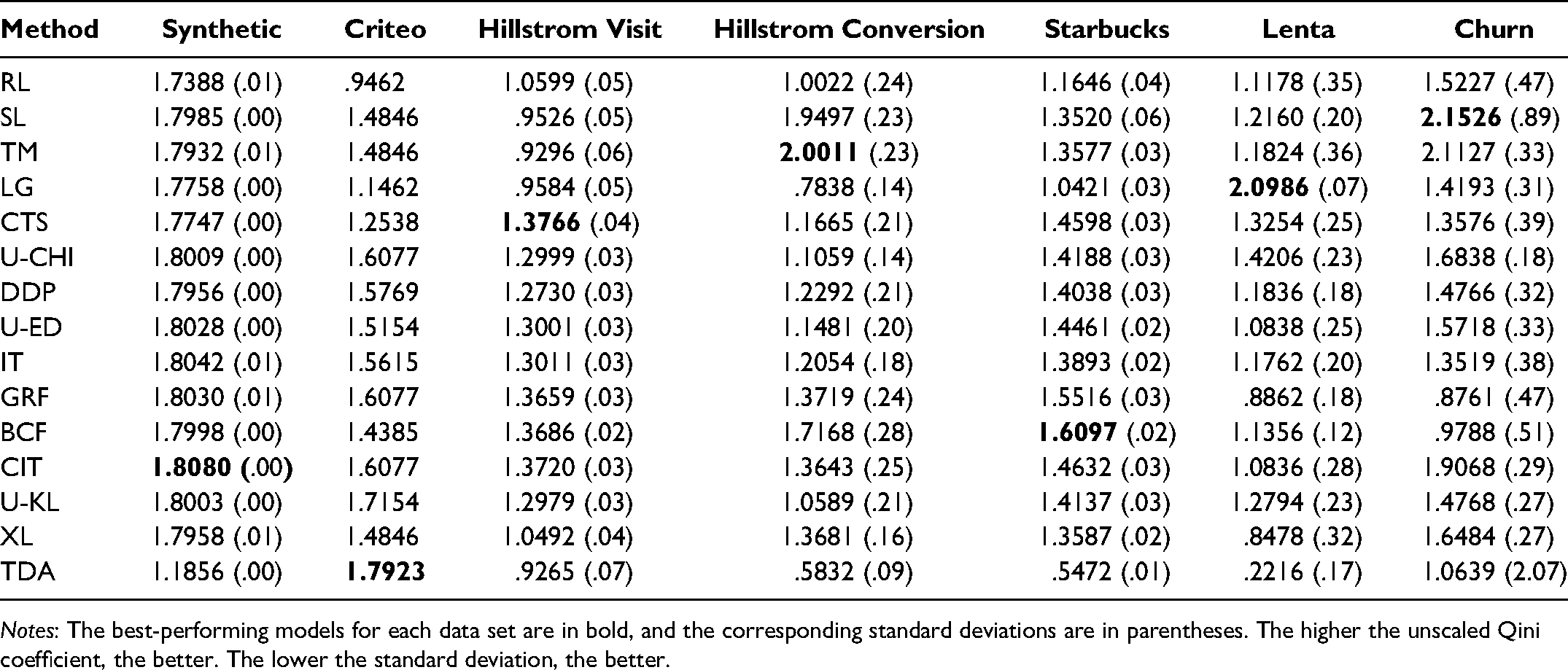
Notes: The best-performing models for each data set are in bold, and the corresponding standard deviations are in parentheses. The higher the unscaled Qini coefficient, the better. The lower the standard deviation, the better.

Average performance

In terms of the (average) unscaled Qini coefficient, CIT, uplift random forests with chi-squared divergence (U-CHI), BCF, and uplift random forests with Kullback–Leibler divergence (U-KL) were the best-performing methods across all data sets (see Table 5). CIT performed very well on most data sets but was only mediocre on Hillstrom Conversion. Although U-CHI did not perform best on any data set, this method achieved high (average) unscaled Qini coefficients on most data sets and performed only (relatively) low on one data set (Hillstrom Conversion). BCF achieved the best score on the Starbucks data set and very good average unscaled Qini coefficients on the Hillstrom Visit data set. However, its performance was second-worst on the Churn data set. U-KL obtained good values on most data sets but a bad average unscaled Qini coefficient on Hillstrom Conversion. In contrast, the worst-performing methods were TDA, RL, and LG. TDA achieved the worst average unscaled Qini coefficient on the synthetic data sets and on four out of six real-world data sets. Nevertheless, the method achieved the highest score on the Criteo data set. Similarly, RL performed poorly on most data sets. Although LG performed best on the Lenta data set, its performance on the remaining real-world data sets was poorly.

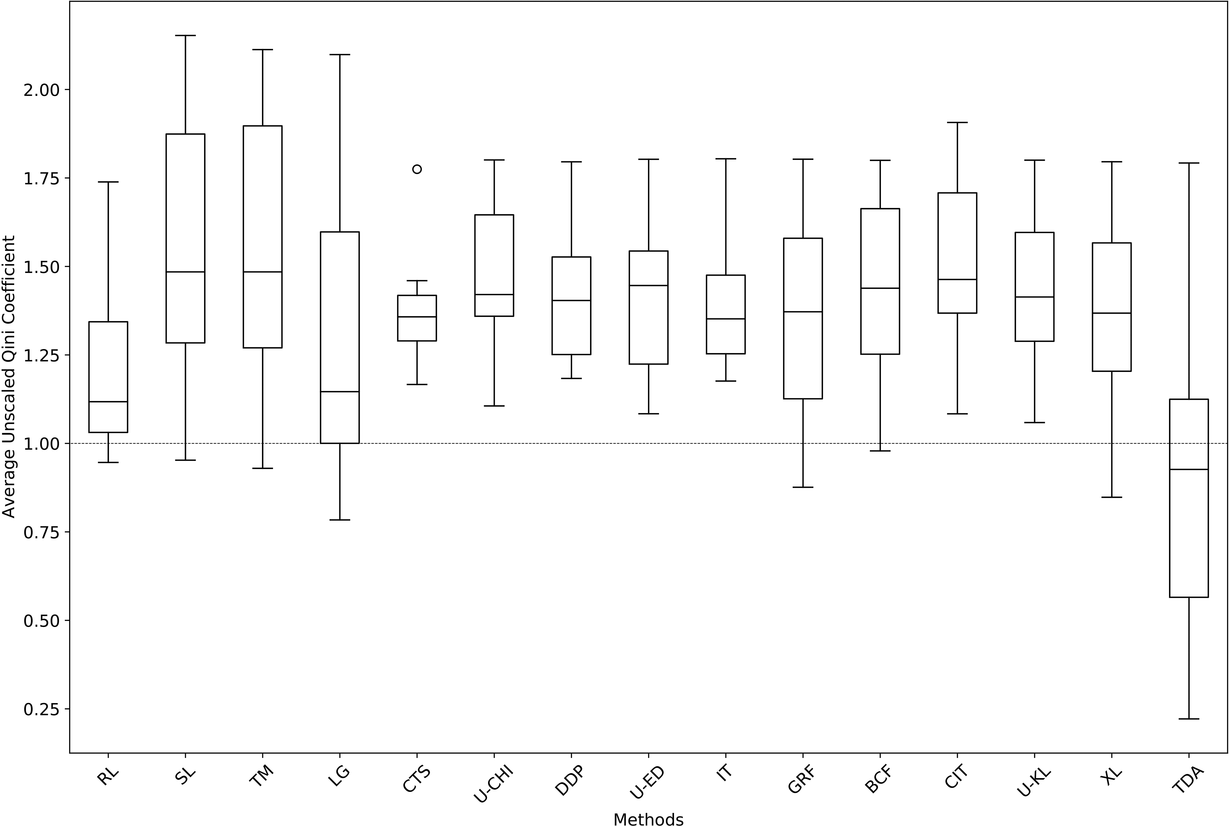
Figure 1 visualizes the performance of all ITE methods across all data sets. Each box plot portrays an ITE method on the x-axis and the average unscaled Qini coefficient across all data sets on the y-axis. Figure 1 shows that all methods performed better than random targeting according to the median in unscaled Qini coefficient, except for TDA, with a median value of .927. It is striking that only seven methods—CTS, U-CHI, DDP, uplift random forest with Euclidean distance (U-ED), IT, CIT, and U-KL—performed better than random targeting on all data sets.

Figure 1.
Average unscaled Qini coefficients of ITE methods across all data sets.

Robustness

In terms of the unscaled Qini coefficient's standard deviation, LG, U-CHI, BCF, U-ED, and DDP were among the best-performing methods (cf. Table 5). Compared with other methods, LG achieved very low standard deviations on all data sets. The performance was only mediocre on the Hillstrom Visit data set. Similarly, U-CHI obtained good values on most data sets. Although BCF achieved the worst score on the Hillstrom Conversion data set, its performance on the remaining data sets was excellent. U-ED and DDP performed similarly well on most data sets except for Starbucks and Lenta. In terms of the unscaled Qini coefficient's standard deviation, RL, TM, and SL were among the worst-performing methods. RL performed poorly on all data sets except for Churn. Similarly, TM obtained high standard deviation values on all data sets except for Starbucks and Churn. SL performed worst on the Starbucks data set, and its performance on Hillstrom Conversion and Hillstrom Visit was also poor.

Looking at the interquartile range in Figure 1, we see that CTS, IT, DDP, U-CHI, and U-KL were the five best-performing methods, while SL, TM, LG, and TDA performed worst. However, although CTS had the lowest interquartile range at .12, note that the method had an outlier at 1.77. In terms of the smallest difference between maximum and minimum, the best five methods were CTS, DDP, IT, U-CHI, and U-ED, and the worst five methods were TDA, LG, SL, TM, and XL (see Figure 1).

Statistical tests

Finally, we applied the Friedman test to the (average) unscaled Qini coefficients and the standard deviation of the unscaled Qini coefficient to examine statistically significant differences among the methods’ performances. Using the unscaled Qini coefficients, we achieved a p-value of .01 for the Friedman test, which led us to conclude that there were statistically significant differences. Thus, we proceeded with the Nemenyi post hoc test to compare all classifiers. We found that U-CHI and CIT performed significantly better than TDA, with p-values of .05 and .01, respectively. Similar to the first test, we obtained a p-value of .01 for the Friedman test when using the standard deviations. Again, we proceeded with the Nemenyi post hoc test and found that U-CHI had a significantly lower standard deviation than RL, with a p-value of .02. We could find no other significant differences.

Qini Curves

In addition to the unscaled Qini coefficient, we assessed model performances by using Qini curves. Recall that these curves display the performance of a method graphically by cumulating the differences in response rate between treatment and control samples as a function of the number of targeted samples (see the “Evaluation Metrics” subsection). Table 6 summarizes the recommended strategies for each real-world data set, including their advantages over targeting all customers. Overall, we can see that, in most cases, companies could have achieved higher response rates while targeting fewer customers. We use the Criteo and Churn data sets to illustrate our procedure here; Appendix B includes detailed explanations for the other data sets.

Table 6.
Recommended Targeting Policies for Each Data Set.

Data Set Recommended Method Customers Targeted (in %) Absolute Number of Contacts Saved Incremental Response Rate Using the Recommended Method (in %) Incremental Response Rate Targeting 100% (in %) Difference in Response Rate (in %)^a

Criteo U-KL 10% 12,549,049 .110 .130 −.020

TDA 50% 6,971,694 .130 .130 +.000

Hillstrom Visit CIT or CTS 50% 9,579 .038 .045 −.007

Hillstrom Conversion TM 20% 15,198 .410 .370 +.040

BCF 80% 3,799 .490 .370 +.120

Starbucks BCF 70% 18,933 1.020 .950 +.070

Lenta LG 20% 106,015 .014 .010 +.004

Churn TM 10% 6,136 .640 −1.480 +2.120

^a
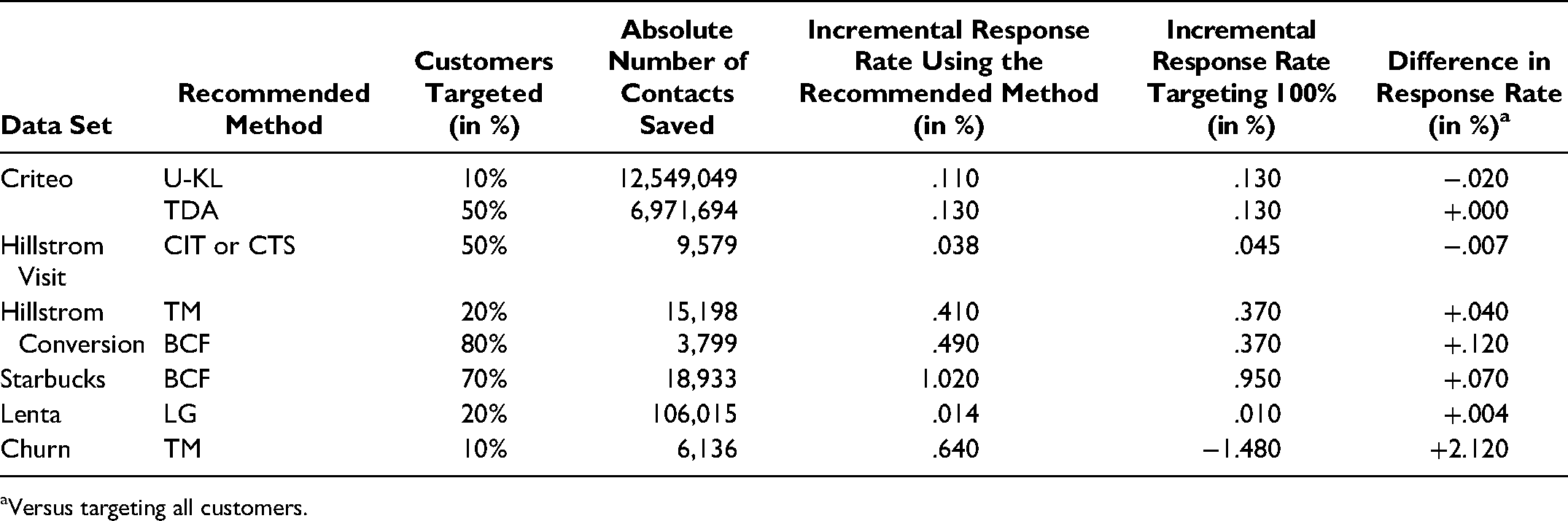
Versus targeting all customers.

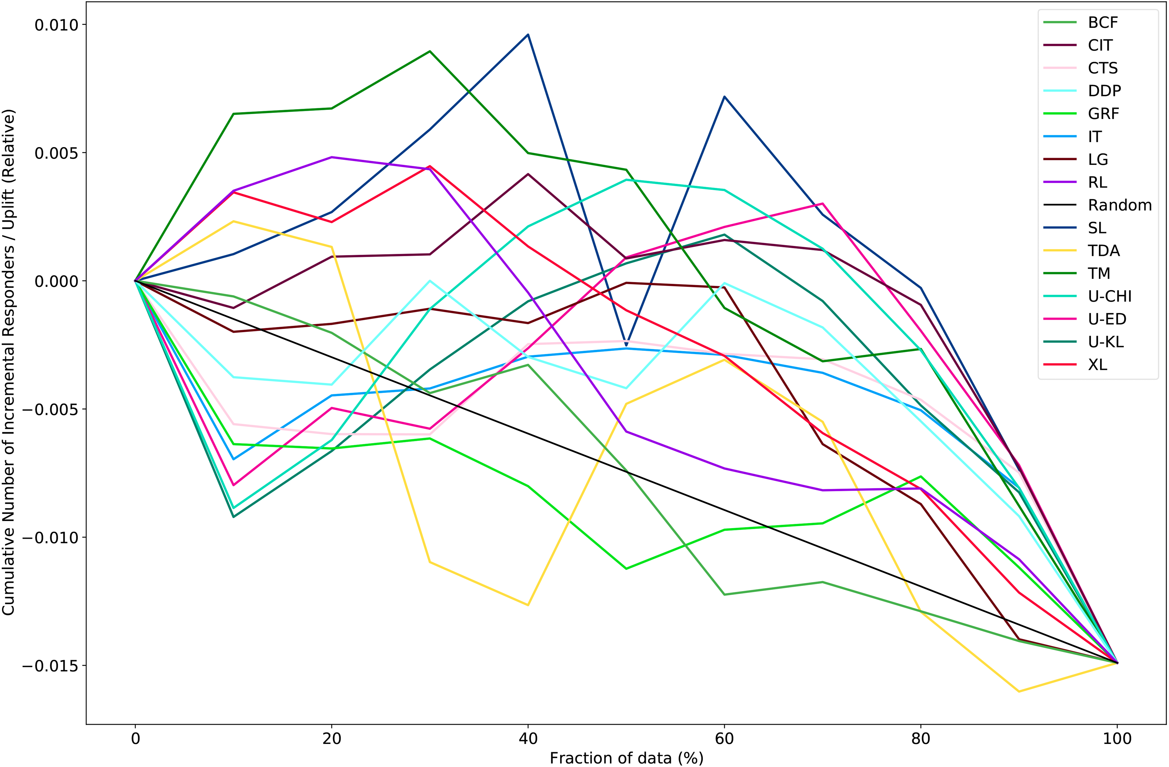
We illustrate the Qini curves for all methods on the Criteo data set in Figure 2. We can see that most of the methods performed better than random targeting. For example, TDA and U-KL were above the random line across all deciles. Further, U-KL achieved 85% of the uplift value in the last decile (uplift: .0013) within the first decile (.0011), and TDA obtained the same uplift value as in the last decile by the fifth decile. Although RL was better than random targeting in the first four deciles, its performance was worse in the last six deciles. Figure 2 shows that one recommended strategy is to use U-KL and target only 10% of the customers, reducing the number of contacts by 90% from 13,943,388 to 1,394,339 while still achieving an incremental response rate of .11%. Another strategy is to use TDA and target only 50% of the customers, achieving an incremental response rate of .13% (compared with an incremental response rate of .13% when targeting 100% of the customers).

Figure 2.
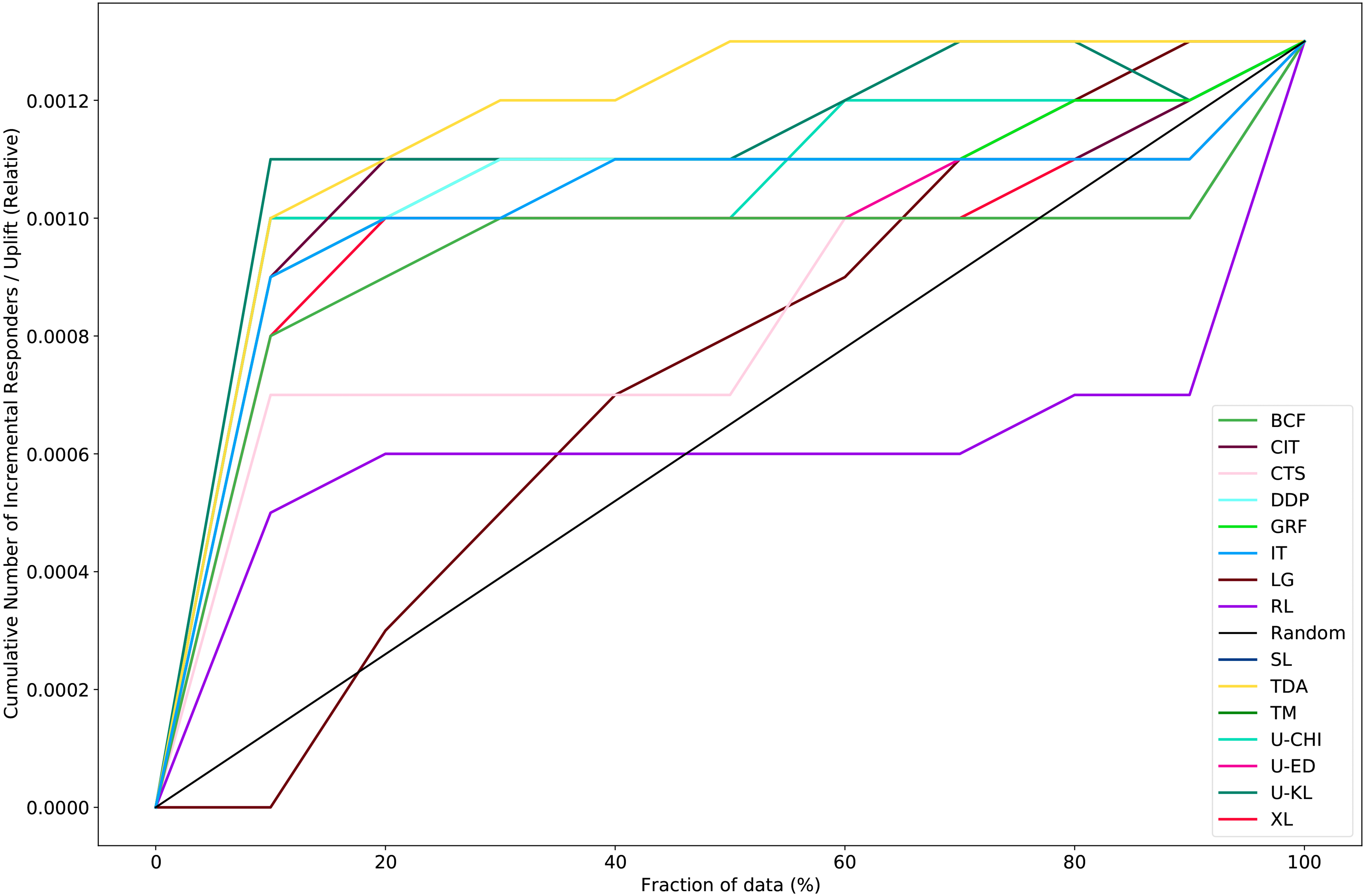
Qini curve on the Criteo data set.

Figure 3 shows the Qini curves for all methods on the Churn data set. We can observe that the performances varied from one decile to another. Further, most methods did not have a “typical” Qini curve, where the uplift value decreased from decile to decile.⁵ For example, U-KL obtained a negative average uplift score of −.009 in the 10% decile but an uplift score of .001 in the 50% decile. Figure 3 reveals that targeting the entire customer base results in a negative uplift value of −1.48%. Recall that targeting costs $40 per individual, and so targeting all 6,818 individuals costs $272,720. One strategy is to use TM to decrease the number of contacts and achieve a positive uplift value. The strategy targets 10% of the customers, thus reducing the number of contacts by 90% from 6,818 to 682 while obtaining a positive incremental response rate of .64%. Compared with targeting all individuals, the company can save $245,440 while obtaining a positive uplift value.

Figure 3.
Qini curve on the Churn data set averaged over the ten test folds.

Conclusion

In this study, we contribute to the optimization of ITEs by comparing methods from two related research streams—uplift modeling and HTE—that until now have been only partially connected. We provide a thorough benchmarking of 15 methods from both literature branches on 27 synthetic and 6 real-world data sets.

In line with current research (Athey and Imbens 2015; Devriendt, Moldovan, and Verbeke 2018; Rößler, Tilly, and Schoder 2021), our results show that most methods suffer from volatility: that is, they perform well for some data sets but poorly for others. We do, however, find that some methods perform better and are more robust than others. U-CHI (Sołtys, Jaroszewicz, and Rzepakowski 2015) is among the best-performing methods in our study. It significantly outperforms TDA and RL in terms of unscaled Qini coefficient and its standard deviation. Further, the method performs better than random targeting on all data sets. Other methods, however, perform only marginally worse. U-KL, as well as U-ED (Sołtys, Jaroszewicz, and Rzepakowski 2015), the BCF (Hahn, Murray, and Carvalho 2020), and CTS (Zhao, Fang, and Simchi-Levi 2017b) also perform very well and robustly in our study. Further, we show that the CIT (Su et al. 2012) and DDP criterion (Hansotia and Rukstales 2002), initially suggested in the form of a CART and CHAID decision tree, respectively, also perform very well and robustly when we use these approaches in the form of a random forest. In contrast, we find that the TDA (Lo 2002), LG (Kane, Lo, and Zheng 2014), and RL (Nie and Wager 2021) are the worst-performing methods, both in terms of predictive power and in robustness. Further, we observe that both baseline approaches, the TM (e.g., Künzel et al. 2019) and SL (e.g., Künzel et al. 2019), have a good predictive power but lack robustness.

As another important finding of our benchmarking study, we highlight that using the incremental effect of a treatment on customer response can substantially improve a targeting policy, but only if we consider methods from both research streams. For example, while the best targeting strategy on the Starbucks data set depends on an HTE method (BCF; Hahn, Murray, and Carvalho 2020), the most promising targeting policy on the Criteo data set depends on an uplift modeling method (either U-KL [Sołtys, Jaroszewicz, and Rzepakowski 2015] or TDA [Lo 2002]).

Similar to Zhang, Li, and Liu (2021), we urge researchers to consider that ignoring the very rich literature on either uplift modeling or HTEs would be a serious omission when making new (methodological) contributions in the context of incremental effect estimation. Further, our study informs practitioners and decision makers in charge of targeting policies that comprehensively assessing targeting policies is possible only if methods from both research streams are considered. Our results show that improving a targeting policy using an ITE method requires evaluating multiple methods from both literature streams. Our results are applicable for organizations that target individuals with specific treatments in various domains such as marketing (e.g., churn management), political science (e.g., political campaigns), and health care (e.g., estimating drug effects).

We are aware that our research has some limitations; these offer excellent avenues for future research. First, while we focus on binary response and binary treatment variables, other researchers could extend our classification to continuous response and multiple treatment variables. Second, although our synthetic data sets demonstrate the usefulness of most algorithms, we could not use the data to derive boundary conditions—that is, for example, finding the circumstances under which the performance of different approaches differs when varying ratios of recipients that exhibit the behavior with or without treatment, or varying levels of ITEs. Thus, other scholars should advance the body of knowledge in this field and examine the data and context dependence of various methods by conducting a simulation-based analysis of boundary conditions. Third, we invite other researchers to combine recent findings from both research streams, form new solutions, and find new insights that would have been impossible with only one research stream. An example would be to combine the “honest” approach from Athey and Imbens (2016) with the split criterion proposed by Rzepakowski and Jaroszewicz (2012). Finally, although we used decile-based metrics (i.e., the uplift curve and the unscaled Qini coefficient), other researchers could assess the algorithms’ performances using an actual versus predicted outcome evaluation. To obtain the ground truth, researchers could, for example, construct more synthetic data sets or create synthetic data sets that resemble the real-world data.

In summary, our study encourages researchers and decision makers in charge of targeting policies to consider both uplift modeling and heterogeneous treatment effects when leveraging the incremental effect of a treatment on customer response.

Study	Short Method Description and Potential Strengths and Weaknesses	Assumptions
Hansotia and Rukstales (2002)	$Δ Δ p$ (DDP): CHAID decision tree (Kass 1980) with a splitting criterion that maximizes the difference of the difference between the treatment and control response probability in the left and right child node (called DDP).Potential weaknesses: Bad performance (Rzepakowski and Jaroszewicz 2012).	Binary treatment, binary response randomization^a
e.g., Künzel et al. (2019)	Two-model approach (TM): Predict ITEs by calculating the difference between estimations from two independent models. The first model estimates the conditional expectations of the outcomes for individuals subject to a treatment, while the second model estimates the conditional expectations of the outcomes for individuals not subject to a treatment. The ITE is then calculated as the difference between these estimates.Potential strengths: Algorithmic flexibility (Devriendt, Moldovan, and Verbeke 2018); good performance if treatment effect is complicated (Künzel et al. 2019).Potential weaknesses: Bad performance if the treatment effect is simple (Künzel et al. 2019).	Randomization^a
e.g., Künzel et al. (2019)	S-learner (SL): Predict the response (Y) using all the independent variables and the treatment indicator (T) as covariates (X). Thus, the treatment indicator (T) is simply used as another covariate.Potential strengths: Algorithmic flexibility (Devriendt, Moldovan, and Verbeke 2018).Potential weaknesses: Can be biased toward 0 (Künzel et al. 2019).	Randomization^a
Kane, Lo, and Zheng (2014)	Lai's generalization (LG): Create a new, transformed outcome variable $Y^{}$ using the response (Y) and treatment indicator (T): $Y^{} = {\begin{matrix} 0 if T = 0 and Y = 1 \\ 1 if T = 0 and Y = 0 \\ 2 if T = 1 and Y = 1 \\ 3 if T = 1 and Y = 0 \end{matrix} .$ Then approximate the ITE by weighting the outcome probabilities with the given treatment–control ratio: $\hat{τ} (x) = E [\frac{P (Y^{} = 2)}{P (T = 1)} + \frac{P (Y^{} = 1)}{P (T = 0)} - \frac{P (Y^{} = 3)}{P (T = 1)} - \frac{P (Y^{} = 4)}{P (T = 0)} \| X_{i} = x] .$ Potential strengths: Bias correction of imbalanced treatment–control ratio (Kane, Lo, and Zheng 2014); algorithmic flexibility (e.g., Devriendt, Moldovan, and Verbeke 2018).Potential weaknesses: Volatile performance (Devriendt, Moldovan, and Verbeke 2018; Gubela et al. 2019)	Binary treatment, binary response randomization^a
Künzel et al. (2019)	X-learner (XL): First, the method models Y_i(1) and Y_i(0) separately using the treatment and control groups, respectively. Second, it imputes the treatment effect for each individual—that is, the difference between the true outcome and the estimated outcome using the control estimator is calculated for the individuals in the treatment group; for the individuals in the control group, the difference between the estimated outcome using the treatment estimator and the true outcome is calculated. The imputed treatment effects D¹ and D⁰ are then used as outcome variables to estimate ${\hat{τ}}_{1} (x) = E [D^{1} \| X = x]$ and ${\hat{τ}}_{0} (x) = E [D^{0} \| X = x]$ using any type of base learner (e.g., decision tree, regression model). Third, the ITE is predicted by weighting the estimates from the second step with a weight function $g \in [0, 1]$ : $\hat{τ} (x) = g (x) {\hat{τ}}_{0} (x) + [1 – g (x)] {\hat{τ}}_{1} (x)$ .Potential strengths: Can adapt to structural properties (e.g., sparsity) (Künzel et al. 2019); good performance when one of the treatment groups is much larger than the other (Künzel et al. 2019); algorithmic flexibility (Künzel et al. 2019).	Binary treatment, randomization^a
Lo (2002)	Treatment dummy approach (TDA): Use covariates (X), treatment indicator (T), and the interaction between covariates and treatment indicator (X × T) as independent variables and the response variable (Y) as dependent variable in a logistic regression to estimate the ITE.Potential strengths: Good performance (Devriendt, Moldovan, and Verbeke 2018; Gubela et al. 2019).Potential weaknesses: Large compound errors and multicollinearity (Devriendt, Moldovan, and Verbeke 2018).	Binary treatment, randomization^a
Nie and Wager (2021)	R-learner (RL): Decompose the CATE function such that it depends on the conditional mean outcome and the treatment propensity. Subsequently, first estimate the conditional mean outcome and the treatment propensity and then estimate the ITE by minimizing the objective function (called R-loss).Potential strengths: Algorithmic flexibility (Nie and Wager 2021).Potential weaknesses: Volatile performance (Imai and Li 2021; Nie and Wager 2021).	Randomization^a
Sołtys, Jaroszewicz, and Rzepakowski (2015) and Guelman, Guillén, and Pérez-Marín (2015)	Uplift random forest: Bagging of CART (Breiman et al. 1984) decision trees with Kullback–Leibler divergence, chi-squared divergence, or squared Euclidean distance as splitting criterion.Potential strengths: Good performance (Devriendt, Moldovan, and Verbeke 2018; Rzepakowski and Jaroszewicz 2012; Sołtys, Jaroszewicz, and Rzepakowski 2015).Potential weaknesses: Volatile performance (Rößler, Tilly, and Schoder 2021).	Randomization^a
Zhao, Fang, and Simchi-Levi (2017b)	Contextual treatment selection (CTS): Random forest with expected response as splitting criterion, which directly optimizes the uplift performance.Potential strengths: Good performance (Zhao, Fang, and Simchi-Levi 2017b).	Randomization^a
Su et al. (2009)	Interaction tree (IT): CART decision tree (Breiman et al. 1984) with G-statistic as splitting criterion, which automatically finds subgroups in which the treatment effect is found prominent as well as subgroups in which the treatment has a negligible or negative effect.Potential weakness: Does not place value on splits that improve the fit (Athey and Imbens 2016).	Binary treatment, randomization^a
Su et al. (2012)	Causal inference tree (CIT): CART decision tree (Breiman et al. 1984) with likelihood ratio test statistic as splitting criterion, which automatically finds subgroups in which the propensity and treatment effect become more homogeneous.	Binary treatment, randomization^a
Athey, Tibshirani, and Wager (2019)	Generalized random forest (GRF): Family of nonparametric estimators that inherit the properties of random forests (Breiman et al. 1984). The estimators can be used for a wide range of statistical settings. When used for heterogeneous treatment effect estimation, the method is very similar to the causal forest method (Wager and Athey 2018). The splitting criterion optimizes splits associated with treatment effect heterogeneity by maximizing the negative expected mean squared error. Further, the authors use different samples for partitioning the covariate space and estimating the CATE scores. Before growing a tree, they split the training sample into an estimation samples, which is used only for CATE score estimation, and a training sample that is used only for selecting tree splits.Potential strengths: Good performance (Athey and Imbens 2016; Hitsch and Misra 2018; Imai and Li 2021; Wager and Athey 2018).	Binary treatment, randomization^a
Hahn, Murray, and Carvalho (2020)	Bayesian causal forest (BCF) model: Decompose the CATE function such that it depends on the prognostic effect (i.e., effect of covariates excluding the treatment variable on outcome) and on the treatment effect. The authors then model the prognostic effect and the treatment effect independently using Bayesian additive regression tree priors.Potential strengths: Good performance (Hahn, Murray, and Carvalho 2020; Imai and Li 2021).	Binary treatment, randomization^a

Data Set	Number of Samples: Treatment/Control	Response Rate Treatment/ Control (in %)	Number of Features	ATE (in %)	Description
Criteo	13,943,388/3,007,301	.31/.18	14	.13	Digital advertising
Hillstrom Visit	19,159/19,072	16.02/11.48	10	4.54	Email marketing campaign
Hillstrom Conversion	18,998/18,926	.98/.64	10	.34	Email marketing campaign
Starbucks	63,112/63,072	1.68/.73	9	.95	Promotional campaign
Lenta	132,519/43,546	.20/.19	110	.01	Promotional campaign
Churn	6,818/6,921	62.03/63.51	34	−1.48	Churn prevention campaign

Method	Base Learner	Abbreviation	Research Stream	Reference
Two-model approach	Random forest	TM	Uplift modeling/HTE (baseline)	e.g., Künzel et al. (2019)
X-learner	Random forest	XL	HTE	Künzel et al. (2019)
Lai's generalization	Random forest	LG	Uplift modeling	Kane, Lo, and Zheng (2014)
Uplift random forest with squared Euclidean distance	Random forest	U-ED	Uplift modeling	Sołtys, Jaroszewicz, and Rzepakowski (2015) and Guelman, Guillén, and Pérez-Marín (2015)
Uplift random forest with Kullback–Leibler divergence	Random forest	U-KL	Uplift modeling	Sołtys, Jaroszewicz, and Rzepakowski (2015)
Uplift random forest with chi-squared divergence	Random forest	U-CHI	Uplift modeling	Sołtys, Jaroszewicz, and Rzepakowski (2015)
Random forest with ΔΔp criterion	Random forest	DDP	Uplift modeling	Hansotia and Rukstales (2002)
Contextual treatment selection	Random forest	CTS	Uplift modeling	Zhao et al. (2017a)
Random forest with interaction tree criterion	Random forest	IT	HTE	Su et al. (2009)
Random forest with causal inference criterion	Random forest	CIT	HTE	Su et al. (2012)
S-learner	Random forest	SL	Uplift modeling/HTE (baseline)	e.g., Künzel et al. (2019)
Treatment dummy approach	Logistic regression	TDA	Uplift modeling	Lo (2002)
R-learner	Random forest	RL	HTE	Nie and Wager (2021)
BCF	Bayesian additive regression trees	BCF	HTE	Hahn, Murray, and Carvalho (2020)
GRF	Random forest	GRF	HTE	Athey, Tibshirani, and Wager (2019)

Method	Synthetic	Criteo	Hillstrom Visit	Hillstrom Conversion	Starbucks	Lenta	Churn
RL	1.7388 (.01)	.9462	1.0599 (.05)	1.0022 (.24)	1.1646 (.04)	1.1178 (.35)	1.5227 (.47)
SL	1.7985 (.00)	1.4846	.9526 (.05)	1.9497 (.23)	1.3520 (.06)	1.2160 (.20)	2.1526 (.89)
TM	1.7932 (.01)	1.4846	.9296 (.06)	2.0011 (.23)	1.3577 (.03)	1.1824 (.36)	2.1127 (.33)
LG	1.7758 (.00)	1.1462	.9584 (.05)	.7838 (.14)	1.0421 (.03)	2.0986 (.07)	1.4193 (.31)
CTS	1.7747 (.00)	1.2538	1.3766 (.04)	1.1665 (.21)	1.4598 (.03)	1.3254 (.25)	1.3576 (.39)
U-CHI	1.8009 (.00)	1.6077	1.2999 (.03)	1.1059 (.14)	1.4188 (.03)	1.4206 (.23)	1.6838 (.18)
DDP	1.7956 (.00)	1.5769	1.2730 (.03)	1.2292 (.21)	1.4038 (.03)	1.1836 (.18)	1.4766 (.32)
U-ED	1.8028 (.00)	1.5154	1.3001 (.03)	1.1481 (.20)	1.4461 (.02)	1.0838 (.25)	1.5718 (.33)
IT	1.8042 (.01)	1.5615	1.3011 (.03)	1.2054 (.18)	1.3893 (.02)	1.1762 (.20)	1.3519 (.38)
GRF	1.8030 (.01)	1.6077	1.3659 (.03)	1.3719 (.24)	1.5516 (.03)	.8862 (.18)	.8761 (.47)
BCF	1.7998 (.00)	1.4385	1.3686 (.02)	1.7168 (.28)	1.6097 (.02)	1.1356 (.12)	.9788 (.51)
CIT	1.8080 (.00)	1.6077	1.3720 (.03)	1.3643 (.25)	1.4632 (.03)	1.0836 (.28)	1.9068 (.29)
U-KL	1.8003 (.00)	1.7154	1.2979 (.03)	1.0589 (.21)	1.4137 (.03)	1.2794 (.23)	1.4768 (.27)
XL	1.7958 (.01)	1.4846	1.0492 (.04)	1.3681 (.16)	1.3587 (.02)	.8478 (.32)	1.6484 (.27)
TDA	1.1856 (.00)	1.7923	.9265 (.07)	.5832 (.09)	.5472 (.01)	.2216 (.17)	1.0639 (2.07)

Data Set	Recommended Method	Customers Targeted (in %)	Absolute Number of Contacts Saved	Incremental Response Rate Using the Recommended Method (in %)	Incremental Response Rate Targeting 100% (in %)	Difference in Response Rate (in %)^a
Criteo	U-KL	10%	12,549,049	.110	.130	−.020
TDA	50%	6,971,694	.130	.130	+.000
Hillstrom Visit	CIT or CTS	50%	9,579	.038	.045	−.007
Hillstrom Conversion	TM	20%	15,198	.410	.370	+.040
BCF	80%	3,799	.490	.370	+.120
Starbucks	BCF	70%	18,933	1.020	.950	+.070
Lenta	LG	20%	106,015	.014	.010	+.004
Churn	TM	10%	6,136	.640	−1.480	+2.120

Footnotes

Appendix A: Training

This appendix details the training and hyperparameter tuning that produced the results reported in the “Results” section.

Appendix B: Qini Curves

This appendix describes the Qini curve analysis on the remaining data sets: Hillstrom Visit, Hillstrom Conversion, Starbucks, and Lenta.

Editor

Sonja Gensler

Declaration of Conflicting Interests

The author(s) declared no potential conflicts of interest with respect to the research, authorship, and/or publication of this article.

Funding

The author(s) received no financial support for the research, authorship, and/or publication of this article.

Notes

References

Ascarza

. (2018), “Retention Futility: Targeting High-Risk Customers Might Be Ineffective,” Journal of Marketing Research, 55 (1), 80–98.

Athey

Imbens

G.W.

(2015), “Machine Learning Methods for Estimating Heterogeneous Causal Effects,” Stat, 26.

Athey

. and Imbens

(2016), “Recursive Partitioning for Heterogeneous Causal Effects,” Proceedings of the National Academy of Sciences, 113 (27), 7353–60.

Athey

Tibshirani

Wager

(2019), “Generalized Random Forests,” The Annals of Statistics, 47 (2), 1148–78.

Breiman

Friedman

J.H.

Olshen

R.A.

Stone

C.J.

(1984), Classification and Regression Trees. New York: Routledge.

Chen

Harinen

Lee

J.-Y.

Yung

Zhao

(2020), “CausalML: Python Package for Causal Machine Learning,” ArXiv, http://arxiv.org/abs/2002.11631.

Coussement

Harrigan

Benoit

D.F.

(2015), “Improving Direct Mail Targeting Through Customer Response Modeling,” Expert Systems with Applications, 42 (22), 8403–12.

Demšar

(2006), “Statistical Comparisons of Classifiers over Multiple Data Sets,” Journal of Machine Learning Research, 7, 1–30.

Devriendt

Moldovan

Verbeke

(2018), “A Literature Survey and Experimental Evaluation of the State-of-the-Art in Uplift Modeling: A Stepping Stone Toward the Development of Prescriptive Analytics,” Big Data, 6 (1), 13–41.

10.

Diemert

Betlei

Renaudin

Amini

M.-R.

(2018), “A Large Scale Benchmark for Uplift Modeling,” in Proceedings of the 24th ACM SIGKDD International Conference on Knowledge Discovery and Data Mining. New York: Association for Computing Machinery, http://ama.imag.fr/∼amini/Publis/large-scale-benchmark.pdf.

11.

Foster

J.C.

Taylor

J.M.G.

Ruberg

S.J.

(2011), “Subgroup Identification from Randomized Clinical Trial Data,” Statistics in Medicine, 30 (24), 2867–80.

12.

Friedman

. (1940), "A Comparison of Alternative Tests of Significance for the Problem of m Rankings," The Annals of Mathematical Statistics, 11 (1), 86–92.

13.

Green

D.P.

Kern

H.L.

(2012), “Modeling Heterogeneous Treatment Effects in Survey Experiments with Bayesian Additive Regression Trees,” Public Opinion Quarterly, 76 (3), 491–511.

14.

Gubela

Bequé

Lessmann

Gebert

(2019), “Conversion Uplift in E-Commerce: A Systematic Benchmark of Modeling Strategies,” International Journal of Information Technology & Decision Making, 18 (3), 747–91.

15.

Guelman

Guillén

Pérez-Marín

A. M.

(2015), “Uplift Random Forests,” Cybernetics and Systems, 46 (3/4), 230–48.

16.

Gupta

Han

B.R.

Kim

S.-H.

Paek

(2020), “Maximizing Intervention Effectiveness,” Management Science, 66 (12), 5576–98.

17.

Gutierrez

. and Gérardy

J.-Y.

(2017), “Causal Inference and Uplift Modelling: A Review of the Literature,” in Proceedings of the 3rd International Conference on Predictive Applications and APIs, 67, https://proceedings.mlr.press/v67/gutierrez17a.html.

18.

Hahn

P.R.

Murray

J.S.

Carvalho

C.M.

(2020), “Bayesian Regression Tree Models for Causal Inference: Regularization, Confounding, and Heterogeneous Effects (with Discussion),” Bayesian Analysis, 15 (3), 965–1056.

19.

Hansotia

Rukstales

(2002), “Incremental Value Modeling,” Journal of Interactive Marketing, 16 (3), 35–46.

20.

Hill

J.L.

(2011), “Bayesian Nonparametric Modeling for Causal Inference,” Journal of Computational and Graphical Statistics, 20 (1), 217–40.

21.

Hillstrom

(2008), “The MineThatData E-Mail Analytics and Data Mining Challenge,” blog entry, Kevin Hillstrom: MineThatData (March 20), https://blog.minethatdata.com/2008/03/minethatdata-e-mail-analytics-and-data.html.

22.

Hitsch

G.J.

Misra

(2018), “Heterogeneous Treatment Effects and Optimal Targeting Policy Evaluation,” SSRN, https://doi.org/10.2139/ssrn.3111957.

23.

Holland

P.W.

(1986), “Statistics and Causal Inference,” Journal of the American Statistical Association, 81 (396), 945–60.

24.

Imai

M.L.

(2021), “Experimental Evaluation of Individualized Treatment Rules,” Journal of the American Statistical Association (published online June 21), https://doi.org/10.1080/01621459.2021.1923511.

25.

Jaskowski

Jaroszewicz

(2012), “Uplift Modeling for Clinical Trial Data,” in ICML 2012 Workshop on Clinical Data Analysis, https://people.cs.pitt.edu/∼milos/icml_clinicaldata_2012/Papers/Oral_Jaroszewitz_ICML_Clinical_2012.pdf.

26.

Kane

V.S.Y.

Zheng

(2014), “Mining for the Truly Responsive Customers and Prospects Using True-Lift Modeling: Comparison of New and Existing Methods,” Journal of Marketing Analytics, 2 (4), 218–38.

27.

Kass

G.V

. (1980), “An Exploratory Technique for Investigating Large Quantities of Categorical Data,” Journal of the Royal Statistical Society: Series C (Applied Statistics), 29 (2), 119–27.

28.

Künzel

S.R.

Sekhon

J.S.

Bickel

P.J.

(2019), “Metalearners for Estimating Heterogeneous Treatment Effects Using Machine Learning,” Proceedings of the National Academy of Sciences, 116 (10), 4156–65.

29.

Lai

L.Y.-T

(2006), “Influential Marketing: A New Direct Marketing Strategy Addressing the Existence of Voluntary Buyers,” thesis, School of Computing Science, Simon Fraser University, https://summit.sfu.ca/item/6629.

30.

V.S.Y

. (2002), “The True Lift Model: A Novel Data Mining Approach to Response Modeling in Database Marketing,” ACM SIGKDD Explorations Newsletter, 4 (2), 78–86.

31.

Nemenyi

P.B

. (1963), Distribution-Free Multiple Comparisons. Princeton, NJ: Princeton University.

32.

Nie

Wager

(2021), “Quasi-Oracle Estimation of Heterogeneous Treatment Effects,” Biometrika, 108 (2), 299–319.

33.

Pedregosa

Varoquaux

Gramfort

Michel

Thirion

Grisel

, et al. (2011), “Scikit-Learn: Machine Learning in Python,” Journal of Machine Learning Research, 12 (85), 2825–30.

34.

Radcliffe

N.J.

Surry

P.D.

(2011), “Real-World Uplift Modelling with Significance-Based Uplift Trees,” White Paper TR, 2011–1. Stochastic Solutions, https://stochasticsolutions.com/pdf/sig-based-up-trees.pdf.

35.

Rößler

., Tilly

Schoder

(2021), “To Treat, or Not to Treat: Reducing Volatility in Uplift Modeling Through Weighted Ensembles,” in Proceedings of the 54th Hawaii International Conference on System Sciences, https://doi.org/10.24251/HICSS.2021.193.

36.

Rubin

D.B

. (1974), “Estimating Causal Effects of Treatments in Randomized and Nonrandomized Studies,” Journal of Educational Psychology, 66 (5), 688–701.

37.

Rzepakowski

Jaroszewicz

(2012), “Decision Trees for Uplift Modeling with Single and Multiple Treatments,” Knowledge and Information Systems, 32 (2), 303–27.

38.

Shaar

., Abdessalem

., and Segard

(2016), “Pessimistic Uplift Modeling,” post-print hal-02376023, https://ideas.repec.org/p/hal/journl/hal-02376023.html.

39.

Simester

Timoshenko

Zoumpoulis

S.I.

(2019), “Targeting Prospective Customers: Robustness of Machine-Learning Methods to Typical Data Challenges,” Management Science, 66 (6), 2495–2522.

40.

Sołtys

Jaroszewicz

Rzepakowski

(2015), “Ensemble Methods for Uplift Modeling,” Data Mining and Knowledge Discovery, 29 (6), 1531–59.

41.

Kang

Fan

Levine

Yan

(2012), “Facilitating Score and Causal Inference Trees for Large Observational Studies,” Journal of Machine Learning Research, 13, 2955–94.

42.

., Tsai

C.-L

., Wang

., Nickerson

D.M

(2009), “Subgroup Analysis via Recursive Partitioning,” SSRN, https://doi.org/10.2139/ssrn.1341380.

43.

Tian

Alizadeh

A.A.

Gentles

A.J.

Tibshirani

(2014), “A Simple Method for Estimating Interactions Between a Treatment and a Large Number of Covariates,” Journal of the American Statistical Association, 109 (508), 1517–32.

44.

Tibshirani

(1996), “Regression Shrinkage and Selection via the Lasso,” Journal of the Royal Statistical Society: Series B (Methodological, 58 (1), 267–88.

45.

Wager

Athey

(2018), “Estimation and Inference of Heterogeneous Treatment Effects Using Random Forests,” Journal of the American Statistical Association, 113 (523), 1228–42.

46.

Zaniewicz

. and Jaroszewicz

(2017), “L p-Support Vector machines for Uplift Modeling,” Knowledge and Information Systems, 53 (1), 269–96.

47.

Zhang

Liu

(2021), “A Unified Survey of Treatment Effect Heterogeneity Modelling and Uplift Modelling,” ACM Computing Surveys, 54 (8), 162.

48.

Zhao

., Fang

Simchi-Levi

(2017a), “A Practically Competitive and Provably Consistent Algorithm for Uplift Modeling,” in 2017 IEEE International Conference on Data Mining (ICDM). Piscataway, NJ: IEEE, 1171–76.

49.

Zhao

., Fang

Simchi-Levi

(2017b), “Uplift Modeling with Multiple Treatments and General Response Types,” paper presented at the 2017 SIAM International Conference on Data Mining (June 30), Philadelphia, https://doi.org/10.1137/1.9781611974973.

Studies and Methods	Benchmarking Studies
	Heterogeneous Treatment Effects			Uplift Modeling
	Imai and Li (2021) [2]	Hitsch and Misra (2018) [2]	Künzel et al. (2019) [2]	Devriendt, Moldovan, and Verbeke (2018) [4]	Gubela et al. (2019) [27]	Kane, Lo, and Zheng (2014) [3]	Rößler, Tilly, and Schoder (2021) [9]	Rzepakowski and Jaroszewciz (2012) [16]	Sołtys, Jaroszewicz, and Rzepakowski (2015) [25]	Zaniewicz and Jaroszewicz (2017) [28]	Zhao, Fang, and Simchi-Levi (2017b) [2]
Heterogeneous Treatment Effects
Hahn, Murray, and Carvalho (2020)[BCF model]	X
Athey and Imbens (2015)[Transformed outcome]		X
Wager and Athey (2018)[Causal forest]		X	X
Athey, Tibshirani, and Wager (2019)[GRF]	X
Hitsch and Misra (2018)[Treatment effect projection]		X
Tian et al. (2014)[Interaction approach]					X
Künzel et al. (2019)[XL]			X
Nie and Wager (2021)[R-learner]	X
Uplift Modeling
Lai (2006)[Lai's method]				X	X	X
Kane, Lo, and Zheng (2014)[LG]				X	X	X
Jaskowski and Jaroszewicz (2012)[Class variable transformation]				X			X			X
Shaar, Abdessalem, and Segard (2016)[Pessimistic uplift]				X	X
Shaar, Abdessalem, and Segard (2016)[Reflective uplift]					X
Sołtys, Jaroszewicz, and Rzepakowski (2015) and Guelman, Guillén, and Pérez-Marín (2015)[U-ED]				X			X		X		X
Sołtys, Jaroszewicz, and Rzepakowski (2015)[U-CHI]				X
Sołtys, Jaroszewicz, and Rzepakowski (2015)[U-KL]				X
Rzepakowski and Jaroszewicz (2012)[Uplift tree]								X
Zhao, Fang, and Simchi-Levi (2017b)[CTS]											X
Hansotia and Rukstales (2002)[DDP]								X
Zaniewicz and Jaroszewicz (2017)[Uplift support vector machine]										X
Lo (2002)[TDA]				X	X	X

Bridging the Gap: A Systematic Benchmarking of Uplift Modeling and Heterogeneous Treatment Effects Methods

Abstract

Keywords

Contribution

Theoretical Background: Uplift Modeling and Heterogeneous Treatment Effects

Related Literature

The Gap in Related Work

Prior work

Methodology

Data Sets

Synthetic

Criteo

Hillstrom

Starbucks

Lenta

Churn

Methods

Evaluation Metrics

Statistical Tests

Results

Unscaled Qini Coefficient

Average performance

Robustness

Statistical tests

Qini Curves

Conclusion

Footnotes

Appendix A: Training

Appendix B: Qini Curves

Editor

Declaration of Conflicting Interests

Funding

Notes

References