



Abstract
Measurement equivalence/invariance (ME/I) is a prerequisite for cross-group comparisons when using survey data. Although popular structural equation modeling software programs, including Mplus and lavaan, enable tests of ME/I using simple commands, identifying noninvariant items when full ME/I is rejected is more challenging. This paper reviews current procedures for identifying noninvariant items, particularly when there are more than two groups. We recommend systematically rotating the reference items and conducting pairwise comparisons on the factor loadings estimated in the configural invariance model and the intercepts estimated in the metric invariance model. The results are then summarized with the list-and-delete method to identify sets of invariant items and clusters of invariant groups. A custom R package, MEI, is developed to implement our recommended procedures. With simple commands, MEI automatically conducts ME/I tests, identifies noninvariant items, and compares latent means with partial measurement invariance. This allows researchers to interpret cross-group comparison results more precisely. Finally, our procedures for testing ME/I from cross-group comparisons and the MEI package are extended to longitudinal studies with panel data, congruence studies with dyadic data, and multilevel studies with nested data.
Keywords
Organizational studies often seek to compare means and/or associations across groups. Such groups may be characterized by demographics (e.g., gender, ethnicity, or nationality), rating sources (e.g., self vs. other; supervisors vs. subordinates), measurement formats (e.g., paper-and-pencil vs. online), individual attributes relative to the social environment (e.g., person-job fit), expectations versus perceptions (e.g., psychological contract), experimental conditions (e.g., control vs. treatment), or time points (e.g., longitudinal panels). However, these comparisons are only meaningful if the constructs being studied demonstrate measurement equivalence/invariance (ME/I) across groups, as any observed differences in means or associations may in fact stem from methodological artifacts, including idiosyncrasies in how distinct groups respond to measurement scales (Meredith, 1993).
Although ME/I is widely accepted as a prerequisite for comparing groups in organizational research (Vandenberg & Lance, 2000), the assumption is often not met in practice (van de Schoot et al., 2015). For example, groups may exhibit differences in their (1) relationships between an item and the latent variable, (2) response sets, or (3) interpretations and expectations of the anchors of response scales, to name a few examples. In such cases, researchers must decide how to proceed when the measurement of variables does not function equivalently across groups. A common alternative is to pursue partial measurement invariance, in which parts of a scale show evidence of ME/I, rather than all of it (Byrne et al., 1989). This involves identifying specific items that are noninvariant, which can inform scale development, assist with theoretical interpretation of noninvariance, and—under appropriate conditions—still enable group comparisons and more precisely identify their limitations (Byrne et al., 1989).
However, despite many widely used statistical software packages automating tests of ME/I, the process of identifying noninvariant items still requires time-consuming manual procedures. This task can become especially challenging when comparisons involve many groups or more complex data structures, such as longitudinal panels (Little, 2024; Ployhart & Vandenberg, 2010), dyadic data (Cheung, 1999), and multilevel models (Tay et al., 2014). The concern is that such onerous manual procedures are susceptible to human error, increasing the risk that noninvariance will go undetected or be incorrectly flagged (Luong & Flake, 2023). The downstream consequences of this can be costly, because any observed differences that appear genuine may in fact be measurement artifacts. In turn, researchers may draw inaccurate theoretical conclusions based on invalid measurement foundations.
In this paper, we review the main approaches for identifying noninvariant items when full ME/I is rejected and evaluate their practical limitations. Building on this review, we recommend a procedure in which researchers systematically rotate reference items and conduct pairwise comparisons of factor loadings and intercepts. These comparisons are then synthesized using the list-and-delete method to determine which items are invariant across groups (Rensvold & Cheung, 2001). To support researchers in implementing these procedures, we introduce MEI, a custom R package that automates the full workflow. Crucially, MEI accommodates comparisons across large numbers of groups and a wide range of complex research designs, including congruence studies, longitudinal panels, and multilevel models. By reducing reliance on manual, error-prone procedures, MEI provides a more efficient and transparent way for identifying noninvariant items, ultimately enhancing measurement precision and strengthening the credibility of group comparisons. Before introducing the technical aspects of MEI, we provide a brief overview of common approaches to ME/I tests.
ME/I Within the Multi-Group CFA Framework
Researchers have employed the classical test theory (CTT) model (Lord & Novick, 1968) and the item response theory (IRT) model (Lord, 1980) to test ME/I. In the CTT framework, researchers test for ME/I using multi-group confirmatory factor analysis (MGCFA) with structural equation modeling (SEM) to examine whether the same factor structure adequately fits each group and whether model fit deteriorates substantially after constraining factor loadings and intercepts to be equal across groups. The focus of MGCFA is on scale-level invariance (Meade & Lautenschlager, 2004) of linear relationships between the item and the latent variable (Raju et al., 2002), which is more suitable for studies with smaller sample sizes and fewer items that examine relationships among multiple variables (Tay et al., 2014). In the IRT framework, researchers conduct differential item functioning (DIF) analyses to compare item discrimination and difficulty parameters across groups (Meade & Lautenschlager, 2004; Reise et al., 1993). The focus of IRT is on detecting item-level DIF (Meade & Lautenschlager, 2004) of nonlinear relationships (Raju et al., 2002), which is more relevant for studies with large sample sizes and a great number of items (Meade & Lautenschlager, 2004) to examine the equivalence of test scores and test items (Tay et al., 2015). Due to the popularity of using SEM for assessing the quality of measurement scales and testing hypotheses about relationships among latent variables, the MGCFA approach is the dominant method for testing ME/I in organizational studies (Cheung & Lau, 2012; Vandenberg & Lance, 2000). Accordingly, we focus exclusively on the MGCFA approach in the current paper.
Within the MGCFA framework, all estimated parameters of a structural equation model can be compared across groups, but only a few are relevant to ME/I. The most fundamental test is configural invariance (Meredith, 1993; Vandenberg & Lance, 2000), which assesses whether the factor structure is equivalent across groups. 1 Failing configural invariance renders further comparisons meaningless (Vandenberg & Lance, 2000). After configural invariance is established, researchers can test for metric invariance (weak factorial invariance; Meredith, 1993), which examines whether factor loadings are the same across groups. In addition to configural and metric invariance, researchers can test for scalar invariance (strong factorial invariance; Meredith, 1993), which examines whether the item intercepts are equal across groups—a requirement for comparing latent means. Cheung and Lau (2012) demonstrate that items with the same factor loadings and intercepts across groups imply the same latent mean difference, allowing researchers to confidently draw conclusions about latent mean differences. If the objective is to compare the structural paths or indirect effects across groups, metric invariance is adequate because the structural model is estimated without the mean structures (item intercepts and latent means). Some researchers also test for strict factorial invariance, which includes configural, metric, scalar, and item residual invariance (Meredith, 1993). Strict factorial invariance implies that the reliability of the variable is the same across groups, allowing the comparison of observed scores. However, if a researcher compares structural paths and latent means using SEM, the invariance of item residuals is unnecessary, as the residuals are already accounted for in the estimation of the structural paths and latent means.
Methods for Identifying Noninvariant Items
When full metric or scalar invariance fails, whether a researcher wants to remove a noninvariant item, use partial measurement invariance in subsequent tests, or interpret the noninvariance, it is crucial to correctly identify the noninvariant item(s). Despite extensive ME/I literature, there are surprisingly few discussions on methods for identifying noninvariant items. A major challenge in identifying noninvariant items is assigning an invariant item as the reference item (Cheung & Rensvold, 1999; Johnson et al., 2009). Thus, researchers have proposed various solutions, including methods that do not require assigning a reference item.
Modification Index (MI) Method
To identify noninvariant items, Byrne et al. (1989) suggest using the MI, which shows an expected reduction in the chi-square value for overall model fit when a constrained parameter is freely estimated. They suggest relaxing the invariant constraints on factor loadings sequentially from a full metric invariance model (in which all factor loadings are constrained to be equal across groups) until the overall model fit is adequate (also known as the backward MI approach). However, Yoon and Millsap's (2007) simulation results show that the MI method is ineffective in identifying noninvariant items and inaccurately identifies invariant items as noninvariant. Since an MI is estimated assuming all other constraints are valid—that is, factor loadings of all other items are invariant across groups—the MI method may incorrectly identify the set of noninvariant items if there is more than one noninvariant item (Cheung & Lau, 2012). Furthermore, some MI values may be very similar, but choosing a different sequence of relaxing the constraints may yield a different set of noninvariant items. Also, the MI method is not practical when there are many groups with large sample sizes, because sequentially relaxing the invariant constraints with many large modification indices to identify all noninvariant items can easily lead to an incorrectly specified model (Asparouhov & Muthén, 2014).
Factor-Ratio Test
To model latent variables, researchers must first provide identification by setting the scale of the latent variables. The standardized latent variable approach sets the variance of the latent variable to one, such that the scale of the latent variables is equivalent to the standard deviation. While this approach appears appealing because factor loadings for all items can be estimated, it is not appropriate for testing ME/I because it assumes that the variances of the latent variables are equivalent across groups (Cheung & Rensvold, 1999). This assumption is often violated, particularly in cross-cultural studies.
Little et al. (2006) introduce the effect coding approach as another way to identify latent variables, in which the sum of the factor-loadings equals the number of items and the sum of the intercepts equals zero. Effectively, the latent mean is defined as the average of item means. While the effect coding approach may offer advantages for interpreting latent means in a single-group context, it is not suitable for cross-group comparisons of associations among latent variables, as the associations in the first group are standardized, whereas those in the other groups are unstandardized (Little et al., 2006). Moreover, effect coding does not allow a model with only one noninvariant item because changes in factor loading (or intercept) for one item will result in changes in the factor loading (or intercept) of at least one other item to maintain the sum of factor loadings (or intercepts) equal to the number of items (or zero).
The most common way to identify a latent variable is to arbitrarily assign an item as the reference item by setting its factor loading to one (Mplus; Muthén & Muthén, 1998–2017, and lavaan; Rosseel, 2012, use the first item of a latent variable as the reference item by default), such that the scale of the latent variable is linked to the scale of the reference item. When testing for ME/I, the underlying assumption is that the factor loadings of the reference item are equivalent across groups. If a noninvariant item is chosen as the reference item such that the factor loadings are set to unity across groups, the factor loadings of all other items will be calibrated accordingly, and the item-level ME/I test results can be very misleading (Cheung & Rensvold, 1999; French & Finch, 2008; Yoon & Millsap, 2007). Similarly, the intercept of the reference item can be set to zero in all groups, such that the latent mean is defined as the observed mean of the reference item (Bollen, 1989), or the latent mean of the first group is set to zero, such that the latent means in other groups are defined as the difference in latent mean from the first group (default in Mplus). Both approaches assume the intercept of the reference item is equal across groups. If a noninvariant item is selected as the reference item, the latent mean difference will be incorrectly calibrated.
To address uncertainty about whether the reference item is invariant across groups, Cheung and Rensvold (1999) propose the factor-ratio test, which examines all possible combinations of the reference item and the argument (another item being tested for invariance). The factor-ratio test results are summarized using the list-and-delete method to identify sets of invariant items (Rensvold & Cheung, 2001). This method requires researchers to first list all possible combinations of invariant items, then delete the sets that contain the noninvariant reference and argument item pair identified by the factor-ratio tests. Finally, researchers select the set with the largest number of invariant items. Although the factor-ratio test does not assume any particular item to be invariant and be used as the reference item, the procedure can be tedious because a total of n(n−1)/2 tests are required when n items are to be tested. For example, a latent variable with five items requires 10 invariance tests.
Direct Comparison Method
Traditionally, full metric invariance was tested by constraining the factor loadings to be equivalent across groups. A likelihood ratio test (LRT) was conducted to compare the model fits of the constrained (metric invariance) and unconstrained (configural invariance) models. If the model-fit drops significantly, the full metric invariance model is rejected, and one could conclude that at least one item has noninvariant factor loadings (Marsh & Hocevar, 1985). A full scalar invariance test can be conducted by adding equality constraints to the item intercepts in the metric invariance model.
A concern with the LRT is that it is sensitive to sample size, such that a large sample size, commonly used in multiple-group analysis, may reject full invariance even when only a trivial difference in an item's factor loading results in a significant LRT (Cheung & Rensvold, 2002). Hence, researchers proposed examining changes in fit indices to evaluate deterioration in model fit after adding equality constraints. For example, Cheung and Rensvold (2002) examine changes in fit indices in a simulation study and suggest that if the CFI is reduced by less than −0.01, the constrained model can be retained and full invariance can be concluded. While their ΔCFI criterion is the most commonly employed change in fit indices approach to test for ME/I, other criteria have also been suggested, such as changes in CFI of −0.002 (Meade et al., 2008), a combination of changes in CFI of −0.01, RMSEA of 0.015, and SRMR of 0.03 (Chen, 2007), and changes in CFI of −0.02 and RMSEA of 0.03 (Rutkowski & Svetina, 2014). Another concern with the constrained model approach to testing ME/I is that it relies on changes in overall model fit after adding equality constraints, but without estimating differences in factor loadings and item intercepts (Cheung & Lau, 2012). Furthermore, the constrained model may fail to converge or yield poor model fit; in such cases, the estimated parameters should not be interpreted.
To overcome the issues of using the constrained model approach to testing ME/I, and the labor-intensive process of the factor-ratio test, Cheung and Lau (2012) suggest testing the invariance of all combinations of reference items and arguments using the bootstrap confidence intervals of the difference in factor loadings (or intercepts) estimated in the configural (metric) invariance model. Instead of estimating multiple models, each with a different item as the reference item, they suggest conducting all tests with one model by creating new parameters equal to the differences in factor loadings (and intercepts) when a different item serves as the reference item. The direct comparison method not only reduces the number of estimated models required for the factor-ratio tests, but also provides estimates (effect sizes) of differences in factor loadings (and intercepts), rather than testing ME/I indirectly via the effect of parameter constraints on model fit.
While the direct comparison method can accurately identify items with noninvariant factor loadings and intercepts, several restrictions limit its application. First, transforming parameters, particularly the item intercepts, is cumbersome and prone to human error when shifting the reference item. Additionally, the list-and-delete method is still necessary to summarize the comparison results and identify the invariant item sets. Finally, the method can only be used to compare two groups. It is unclear how the direct comparison method can be applied when there are more than two groups.
Alignment Method (Approximate Measurement Invariance [AMI])
The objective of the alignment method (Asparouhov & Muthén, 2014) is to compare latent means across multiple groups and to identify sets of groups with AMI for each item's factor loading and intercept. Based on a configural invariance model, the alignment method first transforms the factor loadings and item intercepts using an algorithm that minimizes group differences in both, without altering model fit—analogous to rotations in exploratory factor analysis. The alignment method then compares factor loadings and item intercepts between every pair of groups. For each factor loading and intercept, an initial set of AMI groups with statistically nonsignificant pairwise comparisons in the estimated parameter is generated using a Type-I error of 0.01. The final set of AMI groups is identified by comparing the estimated parameter for each group with the weighted average across the AMI groups. If the difference is not significant at the 0.001 level, the group is included in the final set. Factor means are compared using the transformed configural invariance model, without imposing equality constraints on factor loadings or intercepts. The results of cross-group comparisons are reliable when no more than 25% of items are noninvariant (Luong & Flake, 2023; Muthén & Asparouhov, 2014). Technical details of the alignment method are available in Asparouhov and Muthén (2014), while Luong and Flake (2023) provide an accessible review with sample Mplus syntax.
The advantage of the alignment method is that it automates the more intensive process of identifying noninvariant parameters (Luong & Flake, 2023). Nevertheless, the shortcomings of the alignment method limit its application in organizational studies. First, because the alignment method separately identifies invariant groups for intercepts and factor loadings, groups with significantly different factor loadings may have nonsignificantly different intercepts. Interpretation of latent mean differences for groups with noninvariant factor loadings and invariant intercepts can be misleading because different factor loadings imply that the latent variable is measured on different scales across groups (Cheung & Rensvold, 2000). Second, the final AMI groups identified by the alignment method may be inconsistent with the pairwise comparison results, such that two groups with significantly different intercepts may be classified as holding AMI, while two groups with nonsignificantly different intercepts may be identified as noninvariant (Flake & McCoach, 2018). Third, the alignment method identifies only the set with the largest number of groups with AMI, while ignoring any invariance in the remaining groups. As such, the alignment method does not maximize the number of comparisons available in a sample. Finally, the alignment method compares latent means across groups without constraining factor loadings or intercepts to be equal. The interpretation of latent mean difference can be misleading, particularly for groups with noninvariant items.
Bayesian AMI
Muthén and Asparouhov (2013) proposed using the multi-group Bayesian SEM (MG-BSEM) method to identify an AMI model. 2 The method attempts to maximize the fit of a model that allows for cross-group differences in factor loadings and intercepts, with a predefined variance. That approach was extended by Shi et al. (2017) to identify noninvariant items using a two-step approach. First, identifying an item with the smallest difference in the parameter as a reference item using MG-BSEM, and then identifying the noninvariant item using Bayesian Credible Intervals (BCI). One major challenge of using MG-BSEM to estimate an AMI model is selecting the prior (Pokropek et al., 2020). A misspecified prior will result in less precise BCI and posterior standard deviations. In searching for the prior, Muthén and Asparouhov (2013) suggested starting with a full invariant model (prior equals zero) and gradually increasing the prior until a significant improvement in model fit is achieved. Pokropek et al. (2020) noted that defining the improvement in fit is still in its early stages. They ran simulations across several AMI models to recommend thresholds for improvement in fit under various conditions. However, they also cautioned that much more research is required to identify the threshold for models that fail AMI. More recently, Lai et al. (2022) conducted several simulation studies to compare the performance of the Modification Index method, the Alignment Method, and various MG-BSEM methods, including the Bayesian version of the alignment method with noninformative priors (BAO), Bayesian approximate invariance with alignment (BAIA) and the two-step Bayesian approximate invariance with alignment (BAIA-2S). They concluded that the Alignment Method performs best, whereas all BSEM approaches, except for BAO with large samples, perform poorly in comparing structural parameters across groups.
In short, the MG-BSEM has potential, but its application remains limited until more evidence and user-friendly procedures are developed to demonstrate its applicability in testing ME/I in organizational studies. Moreover, most organizational researchers remain unfamiliar with Bayesian analyses and continue to adopt a frequentist approach in their studies, using the maximum likelihood (ML) estimator for SEM. Requiring them to test invariance with the Bayesian approach when estimating structural parameters with the ML estimator raises concerns; requiring them to use Bayes to estimate the structural parameters is also challenging.
Multiple Testing Method Based on False Discovery Rate
Many methods for identifying non-invariant items involve multiple comparisons on the same dataset, which raises concerns about an inflated overall Type-I error. Various procedures for controlling the overall Type-I error rate have been proposed. For example, Byrne et al. (1989) suggest relaxing the constraint on a parameter when the MI is greater than 5.00 (p = .025), rather than 3.84 (p = .05). Cheung and Lau (2012) suggest using the Bonferroni adjustment to determine the critical p-value for each pairwise comparison to control the family-wise error rate (FWER) in the direct comparison method. Asparouhov and Muthén (2014) suggest using a critical p-value of .01 for pairwise comparisons to generate the initial invariant set and a critical p-value of .001 to determine the final invariant set, regardless of the number of items or groups involved in the ME/I test.
Raykov et al. (2013; 2018) demonstrate the application of the Benjamini-Hochberg (B-H) method (Benjamini & Hochberg, 1995) to address multiple comparisons in identifying noninvariant items in testing ME/I. The B-H method applies a sequential Bonferroni-type procedure to control the false discovery rate (FDR), the rate at which multiple null hypotheses are falsely rejected. Benjamini and Hochberg (1995) demonstrate that their procedure yields substantially higher statistical power than the Bonferroni adjustment in multiple comparisons. Raykov et al.'s (2013) application of the B-H method is essentially similar to the MI approach for identifying noninvariant items, starting with a fully constrained model and relaxing/testing the factor loading or intercept for noninvariance one by one. There are multiple concerns about their approach. First, like the MI approach, it fails if there is more than one noninvariant item, since each test assumes that all other parameters are invariant. Moreover, the fully constrained model may yield a poor fit when multiple items have noninvariant factor loadings/intercepts (Zhang & Yang, 2022). Besides, the B-H method assumes a strict condition of positive dependence through stochastic ordering (PDS); otherwise, it is not guaranteed to control the Type-I error rate (Gou, 2024). However, testing the PDS assumption is complicated, and Raykov et al. (2013; 2018) and Zhang and Yang (2022) have ignored it. Finally, the B-H method determines the critical p-value after all comparisons are conducted, which violates the foundation of statistical tests that the Type-I error rate or the critical p-value should be determined before a test is conducted. The negative consequences of post hoc p-value determination in the B-H method are underexplored.
Other Methods
Jung and Yoon (2016) also suggest the forward CI method for identifying noninvariant items. The forward CI method is, in fact, the direct comparison method suggested by Cheung and Lau (2012), but it does not alternate items as the reference item, as the forward CI method assumes the reference item is invariant. This assumption is problematic because it is not possible to tell if an item is invariant before testing, which is why the factor-ratio test and the alignment method were developed. Jung and Yoon's (2016) simulation results show that the factor-ratio test performs better than the forward CI and backward MI methods in controlling the item-level Type-I error rate, but all three methods fail to control the model-level Type-I error rate. However, their simulation results for the factor-ratio test are inaccurate because they did not properly summarize the test's results. The same problem was observed in French and Finch's (2008) study, which did not summarize the results of various pairwise comparisons.
Raykov et al. (2012) also suggest that testing ME/I with competing models is unnecessary. Once the configural invariance model has an adequate fit, then constrain the factor loadings and intercepts to be equal. If that constrained model also provides an adequate fit, proceed with comparisons of latent means and the variance-covariance matrices across groups. However, a good model fit of the fully constrained model does not imply that all factor loadings and intercepts are equivalent across groups. As shown in their example, the Chi-square change between the constrained and unconstrained models is 16.248 with eight degrees of freedom (p = .039), indicating that ME/I should be rejected.
Recommended Procedures for Testing ME/I and Identifying Noninvariant Items
Based on Cheung and Lau's (2012) direct comparison method, we recommend the following measures to address the limitations of current procedures in testing ME/I and identifying noninvariant items, particularly when three or more groups are involved.
Testing Configural Invariance
While most researchers test configural invariance by examining overall model fit in a multigroup analysis, there is concern that, as the number of groups increases, a poor model fit in one group may not be identified in the overall fit indices, particularly when the model fits the data well in other groups. Hence, configural invariance should be tested by examining the model fit of the measurement model for each group independently, since configural invariance implies that the same measurement model fits all groups well.
Overall Model Fit of the Configural Invariance Model
Although the chi-square test was initially used to evaluate the overall fit of a model, it has been criticized for testing a model with a perfect fit (i.e., the fitted covariance matrix is precisely the same as the observed covariance matrix) and for being sensitive to sample size (Cheung & Rensvold, 2001). Recently, following Kline's (2016) recommendation, most organizational researchers report comparative fit index (CFI), Root Mean Square Error of Approximation (RMSEA), and Standardized Root Mean Squared Residual (SRMR) and evaluate model fit using the combination criteria (CFI ≥ 0.95, RMSEA ≤ 0.06, and SRMR ≤ 0.08) proposed by Hu and Bentler (1999). However, because fit indices are influenced by model complexity and other model parameters, scholars have cautioned that Hu and Bentler's (1999) proposed cutoffs may not apply to scenarios outside those in their simulations (Groskurth et al., 2024). As a result, different criteria for evaluating model fit under various conditions have been proposed (e.g., Groskurth et al., 2024; Hair et al., 2009). Groskurth et al. (2024) further proposed determining cutoff criteria using a regression-based approach that accounts for multiple model parameters. While we recommend that researchers use appropriate criteria to evaluate overall model fit, we would like to stress that all approaches for testing ME/I, including those for identifying noninvariant items, are based on the configural invariance model. Hence, the results of the ME/I tests are more accurate with a configural invariance model that better fits the data.
Identification Approach to Latent Variables
Given the problems with standardized latent variable and effect coding approaches, we recommend using the reference item approach to identify latent variables. To address the concern that the reference item must be invariant, we recommend using the factor-ratio test to evaluate multiple models, each with a different item as the reference. Although this is a tedious procedure, it can be easily implemented using an R software package that we have developed (which we outline in the next section).
Correct Baseline Model for Calculation of Incremental Fit Indices
Because the models are not nested, Widaman and Thompson (2003) argue it is inappropriate to calculate incremental fit indices (e.g., CFI and TLI) using the baseline (null) model with no equality constraints on the intercepts and item residuals when testing a model with equality constraints on the intercepts or item residuals. In line with this, we suggest calculating incremental fit indices for models with constraints on intercepts and item residuals based on a null model with similar constraints. Since this revised baseline model is not readily available in popular SEM software (e.g., lavaan and Mplus), most researchers have ignored the issue when testing for scalar invariance and item-residual invariance.
Confidence Intervals for Comparison of Factor Loadings and Intercepts Across Groups
To conduct the pairwise comparisons recommended in the Direct Comparison method, we suggest using Monte Carlo simulations rather than bootstrapping to estimate confidence intervals of differences in estimated parameters. Based on the parameter estimates and the variance-covariance matrix of the freely estimated factor loadings and intercepts in the configural invariance model (or metric invariance model), one million sets of factor loadings and intercepts are simulated, and the confidence intervals of pairwise differences in factor loadings and intercepts between groups are calculated. Monte Carlo simulation is preferred over bootstrapping because bootstrapped samples often yield nonadmissible or improper solutions in the multiple-group context. Monte Carlo simulation should be used when data are nested because the (nonparametric) bootstrapping is improper for nested data (Efron & Tibshirani, 1993). Since our recommended procedure assumes only multivariate normality of the estimated parameters (as in all significance tests for estimated parameters) and makes no additional assumptions about the raw data beyond those for ML estimation in SEM, it is appropriate for nested data, as in multilevel studies. A similar procedure has been used to estimate the confidence intervals of indirect paths in multilevel models (Preacher & Selig, 2012). Tofighi and MacKinnon (2016) demonstrate in their simulation study that Monte Carlo confidence intervals perform at least as well as bootstrapped confidence intervals and, in some conditions, better, in terms of Type-I error, power, and coverage. Moreover, both methods yield confidence intervals that perform better than those produced by the asymptotic delta method. Additionally, the Monte Carlo approach is a lot more efficient than bootstrapping.
Adjustment to Type-I Error Rate
While the Bonferroni adjustment in the ME/I test controls the FWER and the B-H method controls the FDR, both focus on controlling the critical p-value for (pairwise) comparisons without considering the test's objective, which is to identify noninvariant items. There are actually more pairwise comparisons than the possible number of noninvariant items when there are more than two groups. Hence, we suggest controlling the possible false discovery rate (PFDR) for each latent variable, where PFDR = Type-I error rate (e.g., 0.05) divided by the number of possible noninvariant factor loadings/intercepts. For example, in seven groups with five items, the possible noninvariant factor loading is (5-1)×7 = 28. The critical p-value for PFDR = 0.05/28 = 0.0018. Employing the Bonferroni adjustment, the critical p-value = .05/84 (pair-wise comparisons) = 0.0006, which will result in much lower statistical power. We also suggest controlling for the PFDR separately for factor loadings and intercepts, as these tests are based on different parameters.
Identification of Clusters of Invariant Groups
When more than two groups are tested for ME/I, for each combination of reference item and argument, we recommend conducting pairwise comparisons across groups first. Then, applying the list-and-delete method (Rensvold & Cheung, 2001) to identify the set of invariant groups, because that is more accurate and avoids unnecessary tests, as in the alignment method. After identifying the sets of groups with invariant factor loadings or intercepts in each pair of reference and argument items, the model with the least number of freely estimated factor loadings and intercepts (the most parsimonious model with the greatest number of invariant items) will be selected. When multiple models have the same number of estimated parameters, the model with the best fit should be selected.
Summary of Procedures
In summary, the first step in testing ME/I is to test configural invariance by independently fitting the same measurement model to each group. If the model adequately fits data in all groups, configural invariance is established. Then, a configural invariance model is created by simultaneously fitting the measurement model across all groups using MGCFA. To identify invariant factor loadings across groups for the partial metric invariance model, the second step is to estimate the configural invariance models. The direct comparison method will be adopted to create confidence intervals for pairwise comparisons of factor loadings using Monte Carlo or bootstrapping methods. The list-and-delete method is used to identify the sets of invariant groups for each factor loading. Each partial metric invariance model with a different reference item will be estimated, and the model with the best fit (e.g., the one with the smallest SRMR) will be selected for the next step.
A similar procedure on the partial metric invariance model is recommended to identify noninvariant intercepts for the partial scalar invariance model. An intercept with a noninvariant factor loading will be freely estimated to avoid confusion in interpreting latent mean differences. Finally, the partial scalar invariance model can be used to compare latent means by generating confidence intervals for the difference in latent means via Monte Carlo simulations. In addition to multiple-group comparisons, this suggested procedure can also be applied to longitudinal and multi-level studies.
Testing ME/I Using the MEI Package
The above-recommended procedure for identifying noninvariant factor loadings or intercepts requires systematically rotating each item as the reference item and testing the invariance of the other items as arguments. Since this procedure is time-consuming and becomes more complex when involving more than two groups, we developed MEI, an open-source R package, to ease this burden. MEI estimates structural equation models and performs bootstrapping using lavaan, and conducts Monte Carlo simulations with the MASS package (Venables & Ripley, 2002). MEI uses the ML with Robust Standard Errors (MLR) estimator because it is more robust to nested and nonnormally distributed data by adjusting standard errors and fit indices (Maas & Hox, 2004). MEI uses the full-information maximum likelihood (FIML) method, which computes the likelihood for available data to maximize model fit when there are missing values (which should be coded as NA or left blank in the data file).
The package MEI is available on GitHub and can be installed using the following commands in an R console.
One should note that R functions are case-sensitive. Before using MEI, this package needs to be loaded each time the R console is launched with the
In the MEI documentation, Examples A through D illustrate its use in different contexts. Example A demonstrates the use of MEI to test configural, full metric, and full scalar invariance, identify items with noninvariant factor loadings and intercepts, and compare latent means across seven groups. Example B illustrates the use of MEI in a longitudinal study to identify items with noninvariant factor loadings and intercepts, and compare latent means across time. Example C tests for metric and scalar invariance in a congruence study using data from two nonindependent sources. Example D uses MEI to identify items with noninvariant factor loadings across levels in a multilevel model. All datasets for the examples are included with the MEI package, allowing readers to follow the commands in the documentation and work through these examples on their own. We also test for ME/I using the alignment method and Bayesian SEM method in Example A, and the MI method in all examples for comparisons. The MEI Manual, a self-learning kit comprising 2 h of video, PowerPoint slides, data files, and all output files, can be downloaded from the following link: https://osf.io/adt5m/files/xc8k3?view_only=5560c541f2e248c0a37d6bcc9800c1bd/download
In Example A, we simulated a dataset based on the sixth European Working Conditions Survey (Eurofound, 2024) on the life and working conditions of 43,850 respondents in 35 European countries, which we divided into seven regions: North West, Nordic, Continental, Southern, Central East, North East and South East. We examine the ME/I of work-life conflict, engagement and psychological well-being. Work-life conflict was measured by five items (Q45a-e), engagement was measured by three items (Q90a-c) on a 5-point scale (1 = always; 5 = never), and psychological well-being was measured by five items (Q87a-e) on a 6-point scale (1 = all of the time; 6 = at no time).
3
All items were reverse-coded so that higher values indicate higher levels of the constructs. We compare the latent means of work-life conflict, psychological well-being, and engagement across the seven regions. We first calculated the means, standard deviations, and the correlation matrix for the 13 items of each region. Then, we used the LikertMakeR package (Winzar, 2022) to simulate 400 observations for each region in the numerical example. Since the simulated dataset (Example.A) is included in the MEI package, there is no need to load the data file. Otherwise, the first step is to load the data file (Example A.csv) as a data frame.
Next, we define the measurement model (Model.A) with lavaan argument:
Configural, Full Metric and Scalar Invariance
After defining the measurement model, we use the MEI function “Full_MEI” to test for full configural, metric, and scalar invariance of Model.A across the seven regions. The minimum arguments must include the model's name, the data frame's name, and the grouping variable.
MEI first produces the fit indices and estimated parameters for the configural invariance, full metric invariance, and full scalar invariance models. Three summary tables (reproduced as Table 1) at the end of the outputs need special attention. The first table summarizes the model fit indices for the configural invariance, metric invariance and scalar invariance models. Researchers should ensure that the configural invariance model fits the data well because configural invariance is required for all invariance tests. Table 1 shows that the configural invariance model fits the data adequately (
MEI Outputs of the Full_MEI Command in Example A.

The second table displays the differences in fit indices between the metric invariance and configural invariance models, and between the scalar invariance and metric invariance models. We adopted the rule of thumb recommended by Cheung and Rensvold (2002): the more constrained model should be adopted over the unconstrained model if the reduction in CFI is less than −0.01. The change in CFI is preferred to the LRT because it is less affected by sample size than the change in chi-square (Cheung & Rensvold, 2002). In our example with a total sample size of 2,800, even a trivial difference in factor loadings may yield a statistically significant change in the chi-square value. Table 1 shows that adding equality constraints to the factor loadings (Model.metric) reduces the CFI of the configural invariance model by −0.0068, indicating full metric invariance is achieved. Adding equality constraints to the intercepts (Model.scalar) reduces the CFI of the full metric invariance model by −0.0261 (which is more than −0.01), indicating some items have noninvariant intercepts and full scalar invariance is not achieved.
Partial Metric Invariance
The overall test for full metric invariance may not be sensitive enough to reject full ME/I if only a small number of items in a small number of groups are noninvariant (Raykov et al., 2013). In this example, 13 items were used to measure three constructs across seven groups; there could be 60 noninvariant items. Hence, although the previous results indicate that full metric invariance is achieved, we continue to utilize the MEI “CompareLoadings” function to demonstrate its application in identifying items with noninvariant factor loadings. The following command sets the overall Type-I error rate for each construct to 0.05, while adjusting the Type-I error rate for identifying each noninvariant item using the PFDR method. When multiple partial metric invariance models have the same number of estimated parameters, the model with the smallest SRMR is selected as the best fit. Pairwise comparisons are then conducted using confidence intervals generated from one million Monte Carlo simulations (by default).
The MEI outputs will first print out the adjusted Type-I error rate for each invariance test. In this example, the adjusted Type-I error rate for Factors 1 and 3 (each with five items across seven groups) is 0.0021, and for Factor 2 (with three items) is 0.0042. The outputs provide a recommended partial metric invariance model (PMI.Model.R), along with the fit indices and estimated parameters of the recommended model, the differences in fit indices between the partial metric invariance and configural invariance models, and a summary of the estimated factor loadings for the partial metric invariance model. Results from MEI indicate that the factor loadings of items R87b and R87c in the North East region are noninvariant to other regions. The overall fit indices for the partial metric invariance model are
MEI Outputs of the CompareLoadings Command in Example A.
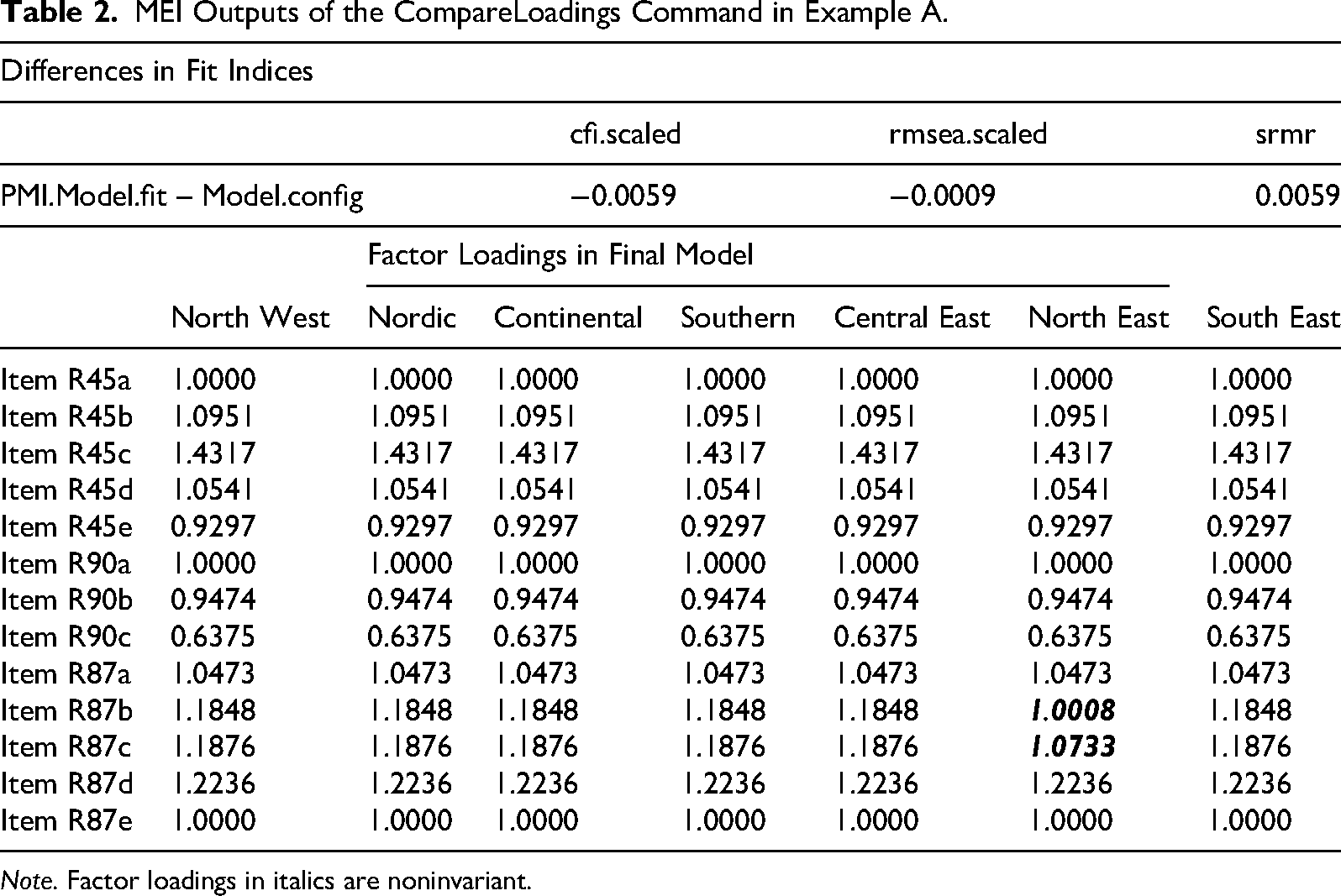
Note. Factor loadings in italics are noninvariant.
Partial Scalar Invariance and Comparison of Latent Means
Next, we use the MEI “CompareMeans” function to identify the items with noninvariant intercepts and compare the latent means with the partial scalar invariance model using the following syntax.
This step is based on the partial metric invariance model (PMI.Model.R) generated in the previous step. MEI outputs will first print out the Type-I error rate used for identifying each noninvariant intercept, followed by a recommended partial scalar invariance model (PSI.Model.R, which is nested within PMI.Model.R), the fit indices and estimated parameters of the recommended model, differences in the fit indices of the partial scalar invariance and partial metric invariance models, and a summary of the estimated intercepts and latent means of the partial scalar invariance model. In this example, each group has 10 freely estimated intercepts (one intercept of each latent variable is fixed to zero to provide identification). There are a total of 70 estimated intercepts (10 × 7 groups), including 10 freely estimated intercepts and 60 possible invariant-constrained intercepts. Results in Table 3 show that the partial scalar invariance model has 50 invariant constraints (differences in df.scale: 542–492 = 50), implying 10 intercepts are freely estimated. The partial scalar invariance model reduces the CFI of the partial metric invariance model by −0.0053, indicating that the invariant constraints on item intercepts are appropriate. For each latent variable, MEI also presents the factor loadings, intercepts, and latent means for each group, along with results of pairwise comparisons of the latent means. We reproduced the results for the factor well-being in Table 3.
MEI Outputs of the Compare Means Command in Example A.

Note. Critical p-value = 0.0024 (0.05/21 comparisons). Differences at p < .0024 are in bold and italics.
Following Cheung and Lau (2012), we recommend interpreting the results of latent mean comparisons only when the majority of items have invariant intercepts. Since there are five items for the factor wellbeing, one should only interpret the latent mean difference if three or more items have invariant intercepts. We recommend using a critical p-value equal to the desired overall Type-I error rate, adjusted for pairwise comparisons of latent means using the Bonferroni method. For example, there are 21 pairwise comparisons for seven groups. To achieve an overall Type-I error rate of 0.05, a critical value of 0.0024 (0.05/21) should be used for each pairwise comparison. Table 3 also shows the latent means and p-values for pairwise comparisons of latent means. The results show that the latent means of the North West (4.3904) and Nordic (4.6223) regions are statistically significantly different (p < .001). Since all intercepts are invariant between these two regions, the latent mean difference can be interpreted without any concern about the differences in psychometric properties of the items.
Although the latent mean difference between the North West (4.3904) and Southern (4.5934) regions is also statistically significant (p < .001), only four items have invariant intercepts between these two regions. The latent mean difference must be interpreted cautiously, and it should be noted that the difference may be an artifact of the differences in the psychometric properties of the noninvariant item between the two regions. Finally, despite the latent mean difference between the Nordic (4.6223) and North East (4.3628) regions being statistically significant (p < .001), this difference should not be interpreted, as only two intercepts (out of five) are invariant across these two regions.
We also use the MI and alignment methods to identify noninvariant items for comparisons. An MI of 10 is approximately associated with a p-value of .001 for a change in chi-square with one degree of freedom. The MI results show that 22 out of 70 constrained intercepts in the full metric invariance model have an MI greater than 10. Relaxing these constrained intercepts one by one to identify the partial scalar invariance model will be tedious and could be subject to human error.
We only discuss the results from the alignment method for the items of well-being as an illustration. The alignment method found that AMI holds for all regions for the intercepts of items R87b and R87e. The alignment method found AMI for all regions, except for the South East region, for the intercept of item R87a. However, the pairwise comparisons from the alignment method also show that the intercepts for the Nordic and Central East regions are statistically significantly different (p < .001).
For the intercept of item R87c, all regions except the North East region have AMI. However, the pairwise comparisons show that the intercepts of the North East and Southern regions are not statistically significantly different (p = .126). Similarly, the intercept is not statistically significantly different between the North East and South East regions (p = .014). For the intercept of item R87d, the alignment method concludes that all regions except Central East have AMI. However, the pairwise comparison results show that the intercepts of North West and South East (p = .000), North West and North East (p = .002), and Nordic and South East (p = .002) are statistically significantly different. In summary, the groups identified to have AMI are inconsistent with the pairwise comparison results. This inconsistency makes interpreting latent mean comparisons more challenging, as they are estimated without constraining factor loadings and intercepts to be equal across groups, thereby violating metric and scalar invariance.
Measurement Invariance Tests in Longitudinal Studies
Recent developments in organizational research have introduced new challenges for popular methods of testing ME/I. One such trend is the rise in longitudinal studies that collect panel data at multiple time points. These panel data can be used to answer many research questions, such as examining the evolution of a variable over time in a simplex or autoregression model (Meredith & Horn, 2001), examining the trajectory of change and identifying the antecedents and consequences of the rate of change using the latent growth model (LGM; Duncan et al., 1994), examining the changes at adjacent time points and investigating whether these changes vary over time using the latent change score model (LCSM; McArdle, 2009), examining multiple variables to investigate potential feedback loops using the cross-lagged panel model (CLPM; Marsh et al., 2005) or the random-intercept CLPM (RI-CLPM; Hamaker et al., 2015), and examining the types of changes (i.e., alpha, beta and gamma changes; Golembiewski et al., 1975) using the ME/I tests (Chan, 1998).
To make an unequivocal conclusion that differences across time are due to changes in the level of variables requires ruling out whether differences are due to changes in the psychometric properties of the variables (Lai, 2023; Little, 2024; Ployhart & Vandenberg, 2010; Somaraju et al., 2022). The ME/I issue is particularly critical in studies that involve relatively rapid changes, such as in children's development, or that span many years (Millsap & Cham, 2012). Ferrer et al. (2008) demonstrate that when full ME/I fails, it is crucial to accurately identify the noninvariant items, as using different items as the reference item may have substantive impacts on the estimated change trajectories. Kim et al. (2020) also demonstrate that if noninvariant items are not correctly identified and freely estimated in a LCSM, even a single noninvariant item can lead to severe bias in the estimated LCSM parameters.
Discussions of ME/I in longitudinal studies with panel data provide the best example of conceptualizing ME/I beyond measurement artifacts that prohibit unequivocal comparisons. Based on response trait theory (Rapkin & Schwartz, 2004; Schwartz & Sprangers, 1999; Sprangers & Schwartz, 1999), Oort (2005) maps different types of response shifts and true change to various ME/I hypotheses. For example, the reconceptualization or redefinition of a construct can be tested by configural invariance, while reprioritization or changes in one's values can be tested by metric invariance. Uniform recalibration or changes in one's internal standards can be tested by scalar invariance, and the invariance of item residual variances can test nonuniform recalibration. Leitgöb and Seddig (forthcoming, as cited in Leitgöb et al., 2023) further decompose a change in the observed mean of an item into four components: recalibration, pure reprioritization, an interaction between reprioritization and the true latent mean change, and the true latent mean change. This decomposition would allow for the comparison of latent means without requiring full metric and scalar invariance. Although the MEI package has not yet fully implemented Leitgöb and Seddig's decomposition model, it provides efficient and effective methods for conducting pairwise comparisons between time points and summarizing the results, which are essential for the decomposition model.
While the MGCFA estimates a measurement model for each mutually exclusive group, panel studies collect data from the same people over time. One nature of panel data is that the same items are used across time, making the data nonindependent. Hence, the residuals of the same items are typically allowed to covary across multiple time points (Lai, 2023).
4
In Example B, we demonstrate the use of MEI to test for ME/I and compare latent means across time. In this example, we simulated a dataset (Example.B) with N = 242 based on the descriptive statistics and correlation matrix of Study 2 in Wu et al. (2009, p. 399). They examined the longitudinal measurement invariance of Diener et al.'s (1985) Satisfaction with Life Scale (SWLS), which consists of five items using a 6-point Likert scale across three time points. The measurement model is defined as follows:
MEI only requires defining the measurement model once. It is unnecessary to define the model for each wave. All items should have the suffixes _T1, _T2, and _T3 (e.g., x1_T1, x1_T2, x1_T3) in the data file to indicate when the item was measured. We examine metric invariance with the following MEI command:
The first argument is the measurement model, followed by the data source and the number of waves. By default, the overall Type-I error rate is set at 0.05, adjusted using the PFDR method, and the best-fit model is selected based on the smallest SRMR. The MEI outputs indicate that a critical p-value of .0062 is used to identify items with noninvariant factor loadings, given the potential to free eight factor loadings.
MEI will create a model with three waves and covary the residuals of all similar items. The results show that the configural invariance model fits the data well (
Next, based on PMI.Model.R, we examine scalar invariance and compare latent means across time using this MEI command:
The model fit of the partial scalar invariance model (PSI.Model.R;
MEI Outputs of the LGCompareMeans Command in Example B.

ME/I in Congruence Studies
Research in congruence, fit, and disagreement presents a special case of testing ME/I for nonindependent samples with only two groups. Many organizational studies compare the ratings of the same set of items directly (e.g., latent congruence model; Cheung, 2009) or indirectly (e.g., polynomial regression; Edwards, 1994) to examine differences in ratings from two sources. Although testing ME/I helps meaningfully examine the sources of misalignment between two rating sources (Cheung, 1999; Tagliabue et al., 2021), many empirical studies that compare dyadic data fail to examine measurement invariance across dyad members (Sakaluk et al., 2021). Because the two rating sources are not independent and the item residuals are correlated across sources, MGCFA is not appropriate for testing ME/I of dyadic data (Claxton et al., 2015). The PAIRCompareLoadings and PAIRCompareMeans functions in MEI can be used to test for ME/I of dyadic data.
In Example C, we demonstrate the use of MEI to test for ME/I and compare latent means across two nonindependent sources, such as data in congruence and fit studies. We simulated a dataset (Example.C) with N = 332 based on the descriptive statistics and correlation matrix reported in Cheung (1999), which are originated from the study by Ashford and Tsui (1991) who asked mid-level executives and their supervisors to rate the executives’ performance using Mintzberg's (1973) 10 managerial roles using a 7-point scale with a higher score represents more effective. The 10 roles were classified into internal and external (Cheung, 1999). The following syntaxes are used to define the model and test for metric invariance in Example C. Since there are only five comparisons for external roles and three for internal roles, we set the Type-I error rate to 0.01.
The results indicate that the configural invariance model provides a good fit to the data (χ2 = 245.97, df = 154, RMSEA = 0.042, CFI = 0.956, and SRMR = 0.046). The metric invariance model (PMI.Model.R) from MEI fits the data well (χ2 = 253.87, df = 162, RMSEA = 0.041, CFI = 0.956, and SRMR = 0.047), yielding a higher CFI by 0.0001 than the configural invariance model. The factor loadings of all items are invariant across the two sources.
Based on PMI.Model.R, the PAIRCompareMeans function is then used to conduct a scalar invariance test and compare the latent means between the two groups. The partial scalar invariance model fits the data well (χ2 = 269.58, df = 167, RMSEA = 0.043, CFI = 0.956, and SRMR = 0.049), and the fit is not substantially worse than the metric invariance model (ΔCFI = −0.0006 and ΔRMSEA = 0.0017). Results in Table 5 show that the partial scalar invariance model has three items with noninvariant intercepts across the two rating sources, two for external roles and one for internal roles. Since more than half of the items for external roles have invariant intercepts, latent mean comparisons are feasible. The results of the latent mean comparison indicate that executives’ self-ratings of external roles (5.2388) are significantly higher (p < .001) than their supervisor ratings (5.0043). Similarly, executives’ self-ratings of internal roles (5.8786) are significantly higher (p < .0001) than their supervisor ratings (5.0769).
MEI Outputs of the PAIRCompareMeans Command in Example C.

Multilevel Measurement Invariance
Another recent trend in organizational studies is to use daily diary or experience sampling methods (ESM) to explore within-person variability in individual attitudes and behaviors (Gabriel et al., 2019). In these studies, the participants respond to the same measures at multiple time points. Although ESM studies primarily focus on examining relationships within individuals using multilevel SEM (MSEM), Preacher et al. (2010) suggest that it is good practice to examine the same structural model at both within- and between-individual levels. Testing the same structural model at both levels allows researchers to examine whether the hypothesized relationships are more stable at the personal level (trait) or fluctuate daily (state), for example, in the case of affective states such as self-esteem. In this context, the ME/I of the multilevel data indicates whether the variables are equivalent across levels (e.g., Sawyer et al., 2022).
While the variables in ESM studies typically have similar psychometric properties across levels, variables in other multilevel studies may carry substantive differences across levels. A measurement concern in such contexts is the risk of atomistic (individualistic) fallacies, whereby relationships or measurement properties observed at the within level (L1) are incorrectly assumed to hold at the between level (L2). In multilevel research, a scale that functions appropriately at the individual level does not necessarily operate equivalently at the team or organizational level. This issue may be particularly salient in team and leadership research, where team-level (L2) constructs are often inferred from individual team members’ (L1) ratings when collective entities cannot directly respond to questionnaires. Although researchers rely on intraclass correlations (ICCs) to justify aggregation, ICCs do not indicate whether the constructs are invariant across levels. Failing to examine ME/I across levels risks committing an atomistic fallacy by conflating individual-level perceptions with team-level constructs.
Lüdtke et al. (2008) distinguished between two ways to aggregate L1 observations to represent L2 constructs, namely formative and reflective aggregation, a distinction that is critical for avoiding such fallacies. Formative aggregation is appropriate for variables that possess configural properties (Klein & Kozlowski, 2000) and are L1-referenced, capturing individual-level attributes whose L2 representations reflect aggregates such as team means or within-team dispersion. In contrast, reflective aggregation is appropriate for variables that exhibit shared properties and are L2-referenced, such that the L2 construct represents a true team-level score and within-team variation is treated as measurement error. For an L2 construct that has shared properties and is aggregated from L1 observations, factor loadings must be invariant across levels to establish psychometric isomorphism (Tay et al., 2014).
Since all L1 (within-group) variables are group-mean centered, the intercepts and latent means of all variables at L1 are set to zero. Hence, only configural and metric invariance across levels are tested. Leitgöb et al. (2023) also suggest that a multilevel model can be used to assess ME/I across clusters, which will be particularly useful when there are tens of groups. Specifically, metric invariance among clusters can be examined by testing the equivalence of factor loadings across L1 and L2, whereas scalar invariance can be examined by testing if the item residual variances at L2 are significantly different from zero.
Evaluating the overall model fit of a multilevel model, particularly in assessing the configural invariance model, must be done cautiously. Since the sample sizes in L1 and L2 typically differ substantially, CFI and RMSEA are seriously biased towards misspecification at L1 (Hsu et al., 2015). Hsu et al. (2015) demonstrated, through simulation results, that CFI and RMSEA could identify misspecification only at L1, whereas only SRMR-between could identify misspecification at L2. Hence, we suggest evaluating the model fit of the configural invariance model using SRMR-within and SRMR-between, and selecting the best-fit models based on SRMR. While there are newer approaches developed to evaluate model fit of a multilevel model, such as the two-step approach that first separates a multilevel model into multiple single-level models (Yuan & Bentler, 2007) and the partially saturated models approach (Rappaport et al., 2020; Ryu & West, 2009), their applications in future empirical studies require more evidence to show the effectiveness of these approaches and their availability in popular SEM software.
We demonstrate in Example D how to compare factor loadings across levels using a simulated dataset of 250 subjects based on the daily diary study by Gruszczynska et al. (2021).
5
They used eight negatively worded items from the Oldenburg Burnout Inventory (OLBI) to measure burnout in 235 employees over 10 consecutive working days. The MEI package requires defining the measurement model (Model.D) only once, without specifying the level as below, and it will compare the model across levels.
We used the following MEI syntax to compare the factor loadings across levels:
The first argument is the measurement model, followed by the data source, the clustering variable (“ID”), the alpha level, the method used to control the overall Type-I error rate, and the fit index used to select the best-fitting model. It is worth noting that Monte Carlo simulation should be used for multilevel studies as nested data are involved. We first used PFDR to control for the overall Type-I error rate. The outputs show the critical p-value is .0071 for seven free factor loadings. However, since the results show that the partial metric invariance model does not fit the data adequately (
The MEI results are reproduced in Table 6, which shows that the configural invariance model fits the data well across levels (
MEI Outputs of the MLCompareLoadings Command in Example D.

Discussion
Testing for ME/I is a standard procedure for examining whether the psychometric properties of the measurement items are equivalent before comparing the means and associations of latent variables across groups in organizational studies. When full metric or scalar invariance is not achieved, interpretation of the differences in latent means and structural paths cannot be made unambiguously because the latent variables are operationalized differently (Horn & McArdle, 1992; Vandenberg & Lance, 2000). Researchers often continue with cross-group comparisons using partial measurement invariance by constraining the invariant items to have the same factor loadings and intercepts, while freely estimating the factor loadings and intercepts of the noninvariant items. Contrary to many researchers’ beliefs, partial measurement invariance is not a panacea for failing full invariance because the latent variables being compared are indeed different across groups. Hence, partial measurement invariance should only be employed in cross-group comparisons when more than half of the items are invariant (Cheung & Lau, 2012). The more invariant items, the stronger the inference and the less ambiguous the conclusion about cross-group differences.
Recently, Robitzsch and Lüdtke (2023) argued that partial measurement invariance should not be a prerequisite for meaningful and valid group comparisons for three reasons. First, they argued that noninvariant items are parallel to the item-by-group interactions in item parameters in Analysis of Variance (ANOVA). As such, these item-by-group interactions do not preclude group comparisons since researchers can compute the average effect while accounting for the heterogeneous treatment effects across groups. However, we contend that such an argument may not be justifiable, as in ANOVA, interpretation of the (average) main effects can be problematic when the interaction is significant (Meyer, 1991). Second, they argued that some comparisons require a fixed set of items, and that identifying noninvariant items and comparing across groups on the subset of invariant items is irrelevant (Robitzsch & Lüdtke, 2023). We agree that researchers should not remove noninvariant items before conducting cross-group comparisons. However, it should be emphasized that cross-group differences under partial measurement invariance with the complete set of items may be attributed to differences in the measurement of the latent variables. Finally, they argued that using one set of invariant items in one group comparison (e.g., Poland vs. Germany) and a different set in another (e.g., Poland vs. Austria) could threaten validity. We contend that their example reflects variations in the measurement of variables across the three countries, and that any interpretation of differences in the latent variables should account for these measurement differences.
Alternatively, Asparouhov and Muthén (2014) suggest that cross-group comparisons can be conducted under AMI estimated by the alignment method or the MG-BSEM method (Muthén & Asparouhov, 2013). The major difference between the AMI approach and the partial measurement invariance approach is that factor loadings and intercepts that are not statistically significantly different across groups are allowed to be freely estimated in AMI models, whereas these parameters are constrained to be equal across groups in the partial measurement invariance approach. Hence, the model fit of an AMI model is equivalent to that of the configural invariance model, which is better than the partial metric and partial scalar invariance models.
However, the increase in model fit and improvements in parameter estimates also pose challenges for interpreting cross-group differences. First, the cumulative effects of slight differences in factor loadings and intercepts across all items need to be examined when comparing structural parameters and latent means. Additionally, unlike the partial measurement invariance approach, which uses an invariant item to set the scale and intercept of a latent variable, the AMI model allows the scales and intercepts of the latent variable to differ across groups. Furthermore, future developments are needed to refine the alignment method and the MG-BSEM method, enabling researchers to generate consistent results in more accessible ways.
Recognizing the importance of identifying noninvariant items in cross-group comparisons, we believe our paper makes three main contributions to the organizational methods literature. First, we provide researchers with an overview of the advantages and drawbacks of popular approaches to identify noninvariant items. Second, we extend Cheung and Lau's (2012) direct comparison method to identify noninvariant items in cross-group comparison studies with more than two groups, longitudinal studies with panel data, congruence studies with dyadic data, and multilevel studies with nested data. Despite Cheung and Lau's (2012) direct comparison method and the factor-ratio test compare factor loadings and item intercepts directly without assuming any item as invariant, implementing the procedures can be time-consuming and tedious. Thus, our third contribution is to develop and make freely available an R-based package, MEI, that automates the recommended procedures for testing full configural, metric and scalar invariance, identifying partial metric invariance and partial scalar invariance models, and comparing latent means across groups. Users of the MEI package only need to define the measurement model and input simple commands to conduct the required tests. The MEI package can generate ME/I test results in less than one minute for a simple model and a few minutes for more complex models. It also produces summary outputs that are easy to interpret. In addition, we responded to the call to identify clusters of invariant groups based on ME/I (Leitgöb et al., 2023). Specifically, unlike other approaches that focus on identifying noninvariant items, the MEI package identifies clusters (sets) of invariant and outlier groups. In contrast, the alignment method focuses on identifying the largest set of groups with approximate invariance. Currently, the MEI package can identify up to 12 sets of groups with invariant parameters for each estimated parameter. In other words, the MEI package is accurate for at least 25 groups and for more groups as long as there are no more than 12 invariant sets of groups. The remaining groups will be considered noninvariant when there are more than 12 invariant sets of groups.
Our recommended method and the MEI package currently have a few limitations. First, our discussion primarily focuses on items that are considered continuous. Future development is required to extend the MEI package to test ME/I with dichotomous and ordinal items. Estimating SEM with ordinal data typically involves the polychoric correlation matrix and the weighted least squares (WLS) estimator. Instead of examining the invariance of item intercepts, the thresholds are compared in a scalar invariance test (Millsap & Yun-Tein, 2004). For interested readers, Liu et al. (2017) provide a tutorial on testing ME/I of ordered-categorical measures in the longitudinal study context.
Second, we have not discussed ME/I for second-order constructs, even though many psychological constructs are second-order variables with multiple dimensions. Chen et al. (2005) and Cheung (2008) provide good tutorials on testing ME/I of second-order constructs. However, we anticipate that the MEI package will be extended to include testing of ME/I for second-order latent variables in the near future.
Third, since ME/I is a general concept applicable to many organizational studies, the MEI package can only incorporate models that are most commonly studied and approaches that are open-source, have been validated, and have been applied extensively. Many new approaches proposed in recent years warrant further exploration for their potential to address different organizational research questions. Examples of these new approaches include Marsh et al.'s (2018) alignment-within-CFA (AwC) procedure that extends the alignment method to multiple regression models, Lai's (2023) application of the AwC procedure in growth models, exploratory factor analysis-based ME/I tests (Sterner et al., 2025), and assessing ME/I using moderated nonlinear factor analysis (Bauer, 2017; Kolbe et al., 2024).
Conclusion
ME/I tests are commonly examined in organizational studies to ensure the psychometric properties are equal across groups before conducting cross-group comparisons. When full metric or scalar invariance is rejected, researchers frequently invoke partial measurement invariance for cross-group comparisons, assuming that cross-group differences can be interpreted unambiguously (e.g., Reise et al., 1993). We emphasize that, contrary to popular belief, partial measurement invariance does not imply that cross-group differences can be interpreted unambiguously. More noninvariant items imply a more substantial difference in the operationalization of the latent variable, and it is less clear if any cross-group difference is due to the difference in the level and relationship among latent variables. It is essential to identify noninvariant items to interpret cross-group differences accurately. Researchers are encouraged to interpret the comparison results cautiously and to discuss conceptually possible causes for noninvariance. To borrow an analog frequently used in ME/I, we do not proscribe comparing fruits across groups, but it is best practice to inform your readers that you are comparing apples to oranges.
Footnotes

Ethical Considerations
There are no human participants in this article, and informed consent is not required.
Funding
The authors received no financial support for the research, authorship, and/or publication of this article.
Declaration of Conflicting Interests
The authors declared the following potential conflicts of interest with respect to the research, authorship, and/or publication of this article: An earlier version of this paper (six-page short format) was published in the Best Papers Proceedings of the 85th Annual Meeting of the Academy of Management.