
Abstract
Social signal processing develops automated approaches to detect, analyze, and synthesize social signals in human–human as well as human–machine interactions by means of machine learning and sensor data processing. Most works analyze individual or dyadic behavior, while the analysis of group or team interactions remains limited. We present a case study of an interdisciplinary work process for social signal processing that can develop automatized measures of complex team interaction dynamics, using team task and social cohesion as an example. In a field sample of 25 real project team meetings, we obtained sensor data from cameras, microphones, and a smart ID badge measuring acceleration. We demonstrate how fine-grained behavioral expressions of task and social cohesion in team meetings can be extracted and processed from sensor data by capturing dyadic coordination patterns that are then aggregated to the team level. The extracted patterns act as proxies for behavioral synchrony and mimicry of speech and body behavior which map onto verbal expressions of task and social cohesion in the observed team meetings. We reflect on opportunities for future interdisciplinary or collaboration that can move beyond a simple producer–consumer model.
Keywords
Many research questions in organizational research relate to how members of organizations behave during dynamic social interactions (LeBaron et al., 2018). Among social interaction phenomena in organizations, team interactions are particularly complex and often puzzling for organizational researchers (Waller & Kaplan, 2018). However, researchers need to understand behavioral team interactions in order to understand emergent team phenomena such as intra-team trust, collaborative sensemaking, or team cohesion, all of which originate in team behavioral dynamics. Several scholars have pointed to the benefits of recording audiovisual team interaction data in order to capture rich data on team dynamics over time (e.g., Kozlowski, 2015; Waller & Kaplan, 2018). Empirical studies adopting audiovisual recording and analysis have made important contributions to understanding the micro-level behavioral dynamics that characterize successful team interactions (e.g., Hoogeboom & Wilderom, 2020; Lehmann-Willenbrock & Chiu, 2018; Uitdewilligen et al., 2018). Yet, behavioral team phenomena continue to be difficult to capture. If researchers go to the trouble of gathering audiovisual data on actual team behavior rather than relying on survey-based proxies of behavior (for a detailed critique, see Lehmann-Willenbrock & Allen, 2018), they need substantial resources for annotating the data and quantifying behavioral patterns. Moreover, team behavioral dynamics are fluid and often change from one minute to the next, which requires “high-resolution” research methods with high sampling rates (Klonek et al., 2019).
This paper presents a social signal processing approach that can automatically detect “high-resolution” behavioral team processes from sensor data that is combined with a machine learning algorithm. This approach moves beyond the state of the art in team interaction analysis in several ways. First, social signal processing can incorporate multiple social signals that occur simultaneously during team interactions, whereas researchers pursuing quantitative team interaction analysis typically focus on only one modality and study sequential verbal or nonverbal interaction behavior (for an overview, see Keyton, 2018). Second, “high resolution” is a debatable term in the literature. The state of the art often considers verbal utterances as the smallest temporal unit (cf., Klonek et al., 2019), but behavioral phenomena in complex social collectives such as teams also occur at a much more fine-grained, sub-utterance level of nonverbal behavior (see Müller et al., 2019). Third, the state of the art in team interaction analysis requires intense human effort, in terms of the many hours that go into annotating the interaction data. Social signal processing develops algorithms that can adequately predict such human annotations (or ground truth labels), with the aim of automating these predictions.
With the growth in artificial intelligence in the last decade, many human behaviors can be measured reliably by state-of-the-art machine learning techniques (see Rudovic et al., 2017). The main premise of machine learning in its most basic form is to learn a mapping from some data to an expected outcome or “label.” Mathematically speaking, this involves minimizing an error between a prediction and an actual outcome by adjusting the parameters of this mapping function. When the learning task involves predicting some aspect of a human's social behavior given some behavioral input data, this is known as the research domain of social signal processing, defined as “the computing domain aimed at modeling, analysis, and synthesis of social signals in human–human and human–machine interactions” (Vinciarelli, 2017).
Social signals are constructs that are generated from a constellation of measurable behavioral cues displayed during social interactions, such as facial expressions, gaze, body posture, movement, gestures, and vocal expressions (e.g., speech rate) that produce a response in others (e.g., team members). The data used in social signal processing are often multimodal social signals that have been captured by sensors in the local environment, capturing, for example, (1) video from cameras, (2) audio from microphones, or (3) bodily movement or physiological data from wearable sensors. Relatively simple social cues such as facial action units from video or sentiment from automatically transcribed text can be extracted without additional human annotation, often reaching acceptable degrees of reliability (for an overview, see Burgoon et al., 2017). To study more complex, multimodal social behaviors such as team processes, machine learning algorithms require training by humans to detect meaningful behaviors. Hence, the final ingredient for training a machine to interpret more complex group or team constructs is human intervention. This may initially trigger some disappointment for researchers who are looking for off-the-shelf technology to capture their constructs of interest. However, once there are sufficient interdisciplinary collaborations to generate more robust machine learning approaches, this will catalyze our understanding of team dynamics and temporal linkages between different team processes (and other behavioral interaction phenomena, including leadership, e.g., Fischer et al., 2020; Hemshorn de Sanchez et al., 2022).
In this paper, we showcase the potential of an interdisciplinary social signal processing approach for obtaining new insights into systematic behavioral patterns in teams and other interacting social collectives in organizations. We apply this approach in a field sample of project team meetings, during which we recorded numerous social signals (audio, video, and movement) and annotated the teams’ verbal interaction with the aim to automatically predict moments of high or low cohesion in the meeting from team patterns of extracted social signals. We specify the requirements for multimodal social signal data gathering, explain how to select appropriate time windows, calculate measures of behavioral mimicry based on multimodal sensor data at the team level, and investigate to what extent automatically extracted behavioral mimicry can predict cohesive team interaction behaviors. We discuss the potential as well as the shortcomings and substantial need for additional interdisciplinary or even transdisciplinary work on automatic behavioral modeling approaches to dynamic team interaction phenomena, in the hope that this paper will inspire others to pool their expertise and embrace interdisciplinary research collaboration opportunities in this area.
Detecting Behavioral Mimicry and Predicting Cohesive Team Interaction Using Social Signal Processing
At the outset, we need to clarify that machine learning, which is the method used in social signal processing for making sense of social signals gathered from various sensors, is different from traditional regression analytical methods in several key ways. Statistical modeling approaches such as regression center on the assumption that data are generated by a given stochastic data model. In contrast, supervised machine learning typically uses algorithms for modeling with the assumption that the process that generated the data given a particular ground truth label is unknown. This distinction between machine learning and statistical modeling has been discussed in depth by Breiman (2001), along with the limitations of statistical modeling approaches. However, machine learning algorithms can and do also utilize regression and logistic regression techniques as a basic tool for prediction tasks. For example, machine learning uses linear or logistic regression analysis for supervised learning, in order to fit a function on the available data (e.g., James et al., 2021). One reason for using supervised learning methods such as logistic regression, which we also use in the current study, is that it somewhat circumvents the challenge of interpretability of machine learning models (i.e., explainable machine learning; e.g., Arrieta et al., 2020). Of note, next to supervised learning approaches such as the current study, machine learning can also employ unsupervised, data-driven approaches to discover patterns in the data as well as meta-learning (e.g., Hospedales et al., 2022; Vanschoren, 2019).
Another way to look at the difference between machine learning and statistical modeling approaches such as regression is to consider the types of analysis that can be achieved by each approach. Regression analysis yields insights into generalized behavior that may be more or less helpful for productive collaboration in teams. In comparison, machine learning enables a more personalized analysis approach. Notably, sometimes machine learning produces different findings than regression analysis. This is because machine learning models are capable of accounting for much higher complexity. Moreover, an important distinction between regression analysis and machine learning is that machine learning intends to automate analysis, whereas regression analysis does not. In other words, the promise of machine learning methods in the area of social signal processing is that we will eventually be able to automatically detect meaningful social interaction phenomena, including complex team constructs such as cohesion.
Social signal processing approaches quickly yield a wealth of data. However, in order to advance organizational research using such methods, the extraction and interpretation of social signals should be guided by theoretical constructs. In our case, we focus on team cohesion, which has been researched more extensively than any other team phenomenon. Several meta-analyses support linkages between cohesion and team performance (e.g., Beal et al., 2003; Castaño et al., 2013; Chiocchio & Essiembre, 2009; Evans & Dion, 1991). Cohesion can be defined as a shared bond or attraction among team members that holds the team together and is grounded in task-based or social aspects of team membership (Casey-Campbell & Martens, 2009). Task cohesion refers to a general orientation toward achieving the group's goals and objectives, whereas social cohesion refers to a general orientation toward developing and maintaining social relationships within the group (e.g., Carron et al., 1985).
As is the case for most team constructs, prior empirical work on team cohesion has predominantly relied on self-report survey measures, often with a cross-sectional approach that is difficult to reconcile with the conceptual understanding of cohesion as a dynamic group property (e.g., Kozlowski & Chao, 2012; Salas et al., 2015). In response, recent work has embraced a longitudinal approach to the study of cohesion in teams (Acton et al., 2020; Hill et al., 2019). However, while contributing interesting insights into the development of team members’ self-reported perceptions of cohesion over time, these studies still offer little in the way of actual behavioral expressions of cohesion. To address this shortcoming in the extant literature, scholars have pointed to audio/video recording of team interactions in order to capture rich data on team dynamics over time (Kozlowski, 2015; Kozlowski & Chao, 2012, 2018; Santoro et al., 2015).
We need to emphasize here that the issue of mismatching theory (which specifies behavioral constructs) and empirical investigations of team constructs (which continue to rely on survey-based behavioral proxies) is a pervasive problem in the literature on team processes, as discussed in detail elsewhere (e.g., Kozlowski & Chao, 2018; Klonek et al., 2019; Lehmann-Willenbrock & Allen, 2018). Note that similar discussions are currently led in the leadership literature (Banks et al., in press; Hemshorn de Sanchez et al., 2022). We ask readers to keep an open mind about the potential of social signal processing approaches to address this core issue in the broader organizational behavior literature, and we use the example of team cohesion for demonstration purposes in this regard.
To clarify our methodological focus within the team process literature, we further need to emphasize the distinction between team emergent states (i.e., the traditional conceptual approach to cohesion) and the behavioral processes of emergence that lead to these states. Insights into the latter have much more explanatory value for understanding the core behavioral mechanisms of dynamic team constructs, for example, when aiming to understand how cohesion develops and changes over time (cf., Kozlowski & Chao, 2018). Pentland and Heibeck (2008) discussed the promise of sensor data to understand social phenomena. Since then, sensor data have mainly been used to predict static measures of team constructs (e.g., predicting self-report surveys of cohesion), even in computer science. Moreover, there is an overreliance on controlled, “clean” laboratory settings in social signal processing, given that high-performing machine learning algorithms are easier to achieve in these settings (for an overview, see Müller et al., 2019). Instead, we propose an application to real-life, messy, temporally dynamic processes in teams (cf., Klonek et al., 2019) and increase the challenge from the computer science perspective as well by aiming to predict much more fine-grained instantiations of team cohesion expressions within dynamic team interactions. Müller et al. (2019) provide a detailed discussion of the incompatibility between highly granular sensor data on the one hand and the static, a-temporal nature of traditional quantitative methods on the other hand (as in the case of the survey-based literature on team cohesion). To address this issue, we need to match the criterion for training our machine learning algorithm much more closely to the high resolution of social signals exchanged during team interactions.
Providing a Ground Truth for Behavioral Expressions of Team Cohesion
A criterion is needed for training and developing algorithms that automatically detect and combine social signals and for evaluating their performance. This criterion is called the ground truth for the construct of interest. It requires labeled data that can be taken as definitive and against which the automated system can be measured and trained (e.g., Pantic et al., 2011). To establish such a ground truth, usually behavioral data are collected for which a human expert has provided a judgment of what the machine should predict. This judgment is the “reference” or “ground truth.” A ground truth can be provided by annotating (or rating or coding) observed behaviors during a social interaction, or it can come from self-reported or other-reported survey measures, external ratings, or outcomes such as team performance. Machine learning algorithms try to minimize the discrepancy between the predicted label and the reference or ground truth. Given sufficient training data, such an algorithm can then be used to automatically analyze new data that is similarly distributed. In our case, this means that given acceptable performance, an algorithm developed to detect cohesion can eventually be applied to new datasets for automatically detecting team cohesion without requiring human annotation effort.
Providing a ground truth at the behavioral event level can be a challenge of its own. In our case, we are looking for behavioral expressions of team cohesion as a starting point for a social signal processing approach. Of note, our aim is to pinpoint indicators of cohesion in the team interaction process, whereas most of the extant literature has investigated perceptions of emergent cohesion (i.e., as the result of prolonged team interactions, although the latter are typically not investigated). Hence, we take some liberties in extrapolating from the extant literature. Some of the extant survey-based research points to observable behavioral indicators of task and social cohesion, respectively. Table 1 provides an overview of these findings and shows how we operationalized each finding at the behavioral event level in team interactions, drawing from the literature on behavioral interactions in team meetings.
Expression of Task and Social Cohesion in Team Interactions.
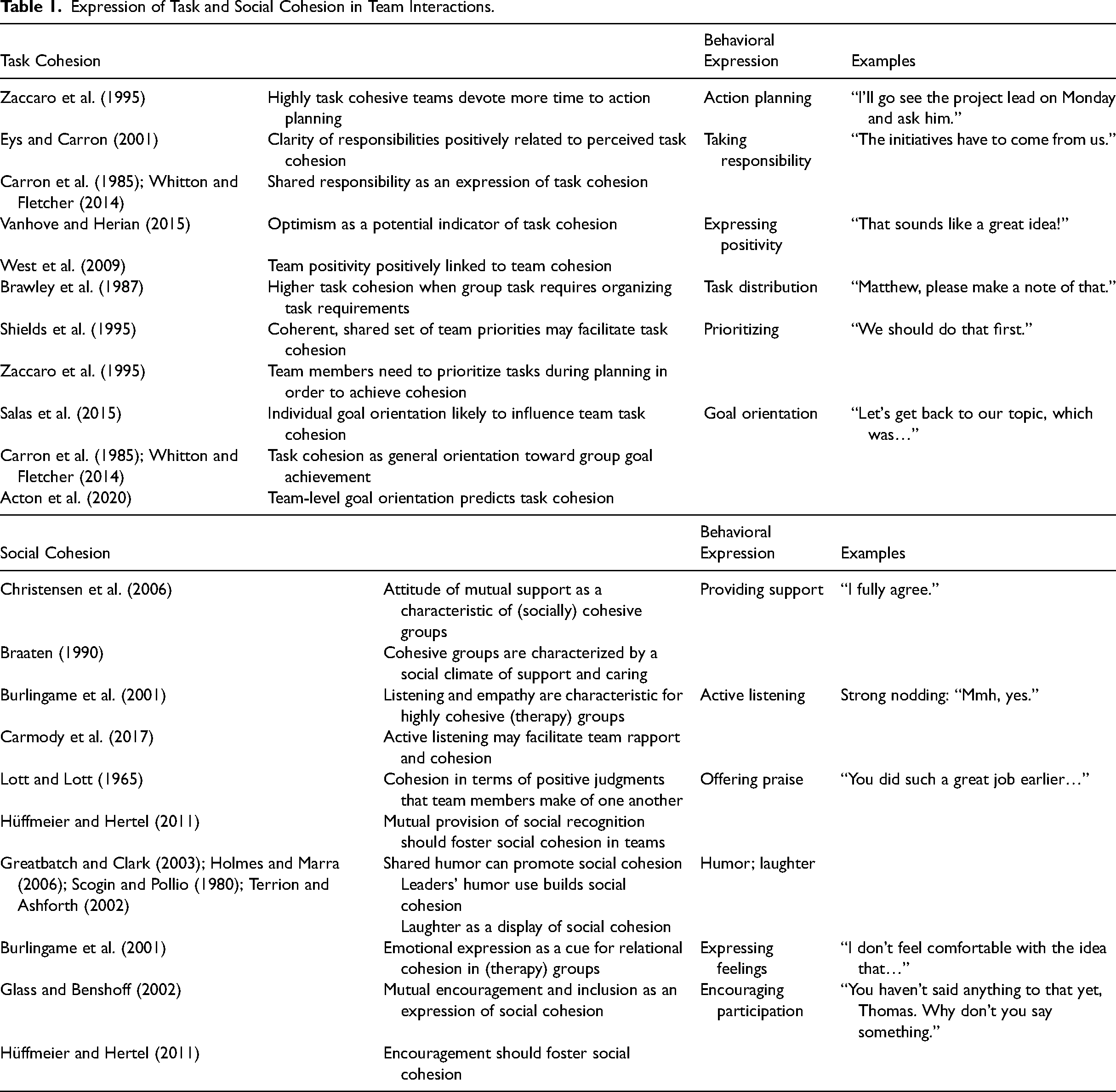
For example, Zaccaro and colleagues (1995) discussed how task cohesive teams devote more time to action planning. In terms of observable verbal behaviors, action planning expresses concrete intentions to act, such as “I’ll take care of this today” or “We’ll have this done by Friday” (e.g., Kauffeld et al., 2018). As further detailed in Table 1, we also include statements that express taking responsibility, such as “This is our job as a team” (e.g., Kauffeld & Lehmann-Willenbrock, 2012), or that signal positivity, such as “This could really work” (Lehmann-Willenbrock et al., 2017). In line with the literature (Table 1), we also consider procedural statements (e.g., Lehmann-Willenbrock et al., 2013) such as distributing tasks, prioritizing, and goal orientation statements as expressions of task cohesion. Regarding social cohesion, we extrapolate from the extant literature as highlighted in Table 1 and consider relational communication such as supportive statements, praise, active listening, expressions of feelings (e.g., Kauffeld & Lehmann-Willenbrock, 2012), humor and laughter (Lehmann-Willenbrock & Allen, 2014), and statements encouraging other members to participate (e.g., “Lisa, what do you think?”) as behavioral indicators of social cohesion in team interactions.
Mimicry and Synchrony of Social Signals
The social signal processing community has frequently considered the role of mimicry or synchrony in social interactions. Mimicry, the interdependence of interacting partners’ behaviors, occurs in almost any social interaction when different individuals converge in their social signals (e.g., Delaherche et al., 2012; Duffy & Chartrand, 2015). Of note, group interactions are considerably more dynamic and complex than dyadic interaction scenarios (e.g., Lehmann-Willenbrock et al., 2017). In thin slices of behavior within the team interaction stream, we show how automatically detected behavioral mimicry based on social signal data can be captured at the group level to predict behavioral expressions of task and social cohesion in team interactions.
Humans have a natural tendency to mimic one another's facial expressions, emotions, speech characteristics and patterns, and motor movements such as posture and gestures (for an overview, see Chartrand & Van Baaren, 2009). Different types of mimicry can be considered behavioral (Chartrand & Lakin, 2013). In other words, mimicry can occur across a range of different behavioral modalities such as gestures, postures, facial expressions, or vocal expressions. In teams, behavioral mimicry occurs when two or more members exhibit similar behavioral patterns within a short time window (i.e., in quick temporal succession, such as a few seconds). In our application example, we use social signal processing to model multimodal mimicry among team members as an underlying mechanism that may help us automatically detect cohesive team interaction behaviors in project team meetings. In other words, when team members mimic their nonverbal expressions and move in sync, this can point to cohesive team interactions.
Research on dyadic interactions has identified several social benefits of mimicry, including increased empathy, bonding, and positive affect (e.g., Stel & Vonk, 2010; Tschacher et al., 2014). Previous research has also found connections between cohesion and behavioral synchrony, defined as the spontaneous rhythmic and temporal coordination of actions between two or more participants (Chartrand & Lakin, 2013; Delaherche et al., 2012; Lakin, 2013; Mayo & Gordon, 2020). Hoehl and colleagues (2021) review and discuss the manifold benefits of synchrony in human interactions, including bonding. Wilson and Gos (2019) found that dyads moving in synchrony are perceived as more cohesive. In the context of large social groups, Jackson and colleagues (2018) showed that behavioral synchrony in movement and arousal increased cohesion. These findings suggest that a social signal processing approach to team interactions should capture mimicry or synchrony.
Whereas some social signal processing work has focused on a single modality only when modeling behavioral mimicry (Nanninga et al., 2017), additional behavioral modalities may need to be considered. Verbal indicators of task and social cohesion (Table 1) may be accompanied by a wealth of nonverbal signals spanning different modalities such as body movement and paralinguistic features (e.g., voice pitch). Taking a step toward multimodal integration, one previous study observed that dyadic mimicry of movement (i.e., accelerometer data) and speech signals, aggregated to the group level, was positively correlated with self-reported task cohesion at the day level (Zhang et al., 2018). Of note, this previous research captured mimicry by aggregating the similarity of participants’ social signals across 10-min periods, which is likely an overly rough time resolution that cannot account for more swift developments and changes in team interaction behaviors. Next, we investigate how social signal mimicry in different behavioral modalities and within fine-grained temporal windows maps onto expressions of task and social cohesion observed in a sample of project team meetings in the field.
Data Gathering
Data were gathered during regular project team meetings at a large software organization in the Netherlands. Our study was endorsed by the local ethics committee as well as the organization's legal department. Participation was voluntary and subject to informed consent by all team members. Data confidentiality was guaranteed. Participants retained the right to withdraw from the data gathering at any time and to have their data deleted upon request. Twenty-five regular meetings were recorded. Meeting size ranged from 3 to 8, with an average of 4.6 attendees. Participants were 64% male, 37 years old on average, with an organizational tenure of 8.6 years and an average team tenure of 2.5 years. To enable multimodal behavioral data gathering, we equipped an on-site meeting room (see Figure 1) with multiple cameras, headset microphones, a microphone array (Microcone; Mast et al., 2015), and a wearable sensor badge. Eight cameras (ABUS HDCC72510, which record at a resolution of 1,920 × 1,080 and at 25 fps), each centered on the seat on the opposite side of the room, were mounted overhead in order to avoid distracting the participants. The Microcone was placed in the center of the table. All individual meeting attendees were outfitted with a microphone (Sennheiser wireless headsets, version ew 152 G3) to record their speech and a custom-built sensor badge worn around the neck measuring torso acceleration at three orthogonal directions of motion. Out of the 25 recorded meetings, 14 had complete data available across all modalities (Table 2).
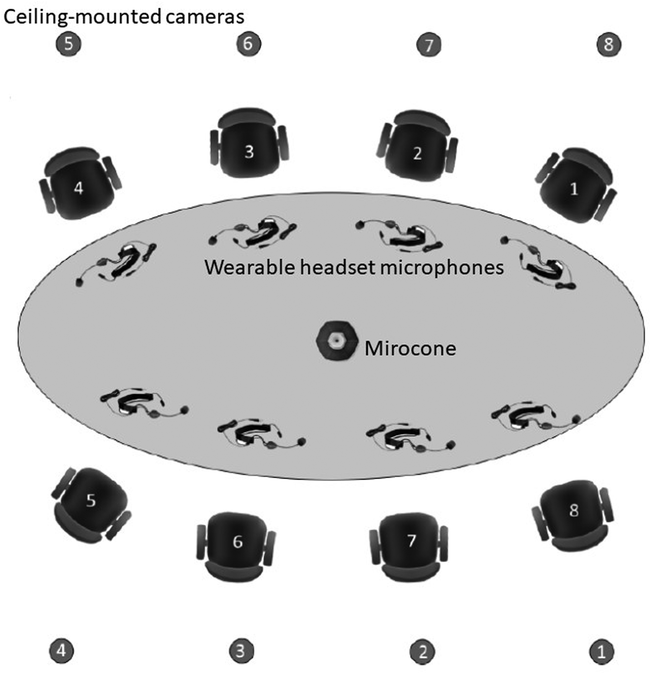
Schematic overview of the on-site meeting room setup showing camera locations, with each camera capturing an individual meeting attendee seated across each camera (1 through 8); wearable headset microphones, one per individual meeting attendee; and the Microcone (microphone array) placed in the center of the boardroom table. Figure adapted from Nanninga et al., (2017). In addition, each attendee wore a custom-built sensor badge around the next to track their motion during the meeting.
Available Sensor Data for Each Modality and Analyzed Meeting Segments Across All Observed Team Meetings.
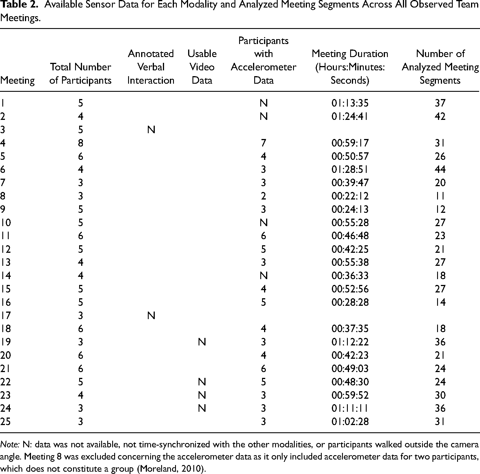
Note: N: data was not available, not time-synchronized with the other modalities, or participants walked outside the camera angle. Meeting 8 was excluded concerning the accelerometer data as it only included accelerometer data for two participants, which does not constitute a group (Moreland, 2010).
Developing Ground Truth Labels
As a ground truth and criterion for training and evaluating our machine learning algorithm, we identified moments of high or low task/social cohesion across 2-min segments of each meeting (in line with previous work on convergent group phenomena; Barsade, 2002). These labels of high or low task and social cohesion were based on the annotated verbal behavior that occurred during each 2-min segment (see Figure 2). Two intensively trained coders annotated the entire stream of verbal interactions using the act4teams coding scheme for team interactions (e.g., Kauffeld et al., 2018), yielding a total of 19,979 verbal utterances. An utterance or sense unit is the smallest speech segment that expresses a complete thought (Bales, 1950). This is often the same as a single sentence, but it can also be a single word (e.g., “Uh-huh” for active listening), leading to a very fine-grained analysis. The final column in Table 1 shows examples of verbal utterances. Like many contemporary studies of behavioral team interactions, the coders used software (specifically, INTERACT software) to annotate directly from the video without needing to transcribe. This creates time stamps with onset and offset times as well as duration for each annotated behavior (for an overview, see Lehmann-Willenbrock & Allen, 2018). Nine randomly selected meetings were annotated twice in order to establish inter-rater reliability for the utterance annotations that were the basis for our ground truth labels (κ = .80).
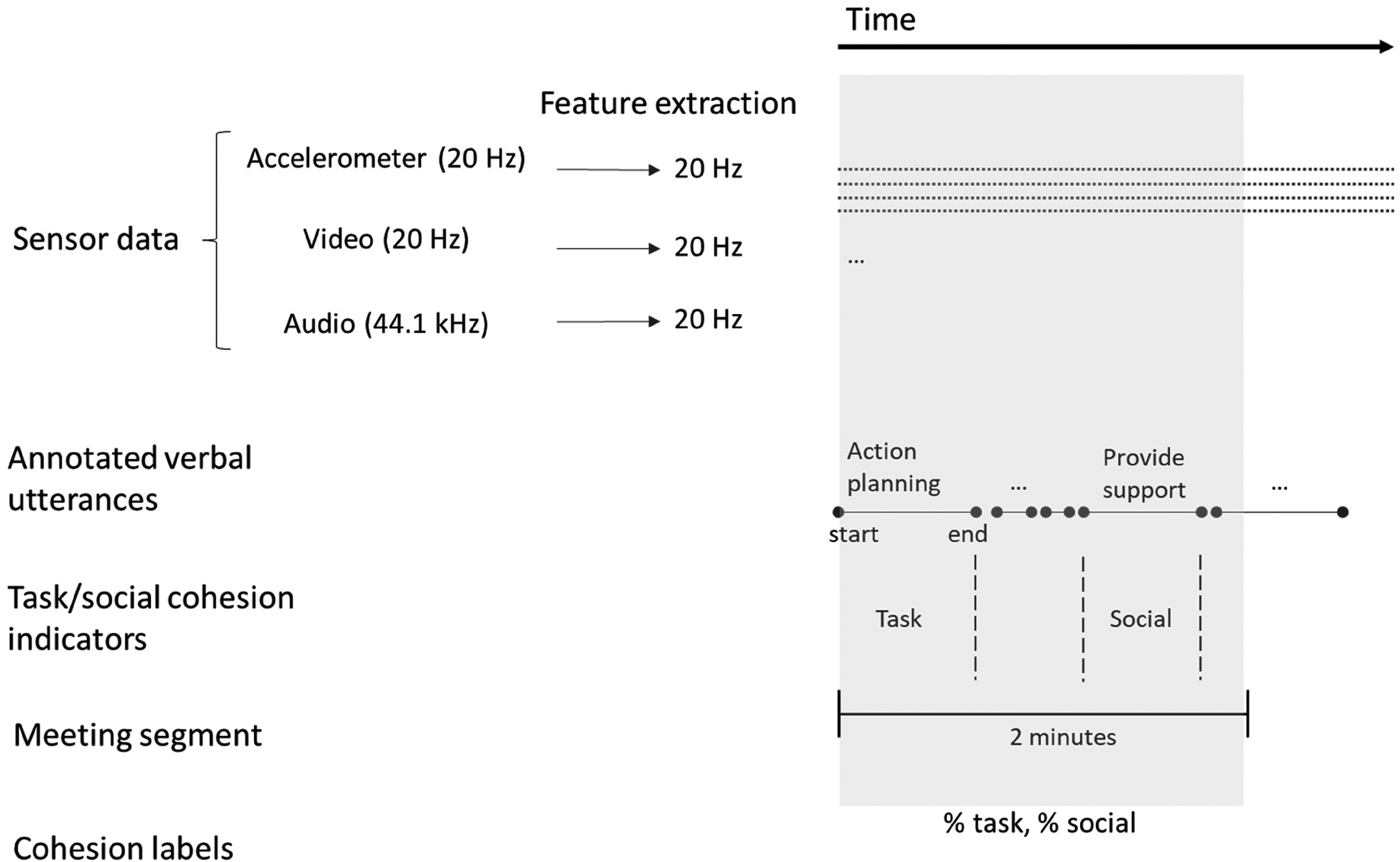
General data gathering framework. Type of data shown on the left and temporal resolution shown toward the right. Sensor data including sampling rates. All features were extracted for 2-min meeting segments within each team meeting (as illustrated by the highlighted section). We extracted 720 features in total (specifics regarding feature extraction are detailed next in the paper). For each 2-min segment, we obtained the ground truth (i.e., cohesion labels) from the annotated verbal utterances, as illustrated in the lower part of the figure. Cohesion labels were obtained at the meeting segment level from the percentages of task and social cohesion behaviors within the respective meeting segment.
To get from the annotated verbal utterances to labels that can be used for social signal processing, we pursued a typical social signal processing approach and labeled the team interaction data using binary ground truth labels for high versus low task and social cohesion, respectively. For each 2-min meeting segment, we computed a proportion of task cohesion and a proportion of social cohesion, based on the verbal behaviors that occurred during each meeting segment (as illustrated in Figure 2). To obtain these labels, we focused on the annotated utterances that indicate task and social cohesion as described in Table 1, third column. From these annotations, for each 2-min segment in each team meeting, we computed the proportion of time that the team spent on these behaviors. We converted these proportions into labels for high and low task and social cohesion by dividing the duration of the verbal behaviors that express task and social cohesion by the duration of all verbal behaviors annotated within each 2-min segment. This produced social and task cohesion values for all 2-min segments of each team meeting which ranged between 0 and 1. Among these values, we defined a “high” label as a value in the top 25% of the distribution and a “low” label as a value in the bottom 25% of the distribution, respectively (for a similar approach, see Hung & Gatica-Perez, 2010). Of note, high task cohesion labels occurred sparsely, whereas moments labeled as high social cohesion were more frequent (see Appendix A for more detail).
Data Processing
In the domain of social signal processing and in machine learning more generally, major time and effort are devoted to pre-processing the gathered sensor data and extracting relevant features from this data (e.g., Khalid et al., 2014; Ramírez-Gallego et al., 2017; Vinciarelli et al., 2009). Hence, we discuss these two aspects of developing a machine learning algorithm for team behavior analysis in detail. Figure 3 provides an overview of our workflow to extract relevant features and automatically predict cohesion labels. The top part of Figure 3 refers to the machine learning approach to the observed team meetings that can account for multiple, simultaneous modalities in team behavior (movement, video, and audio). From the three different modalities, we calculated group-level similarity (i.e., mimicry) values among team members. These values were used to predict high/low cohesion labels. The bottom part of the figure refers to the human analysis of these team meetings. The dotted lines illustrate how we obtained ground truth labels for task and social cohesion from the human annotations of the observed team meetings. These labels served as criteria for training and evaluating the machine learning algorithm for automatically detecting cohesion.
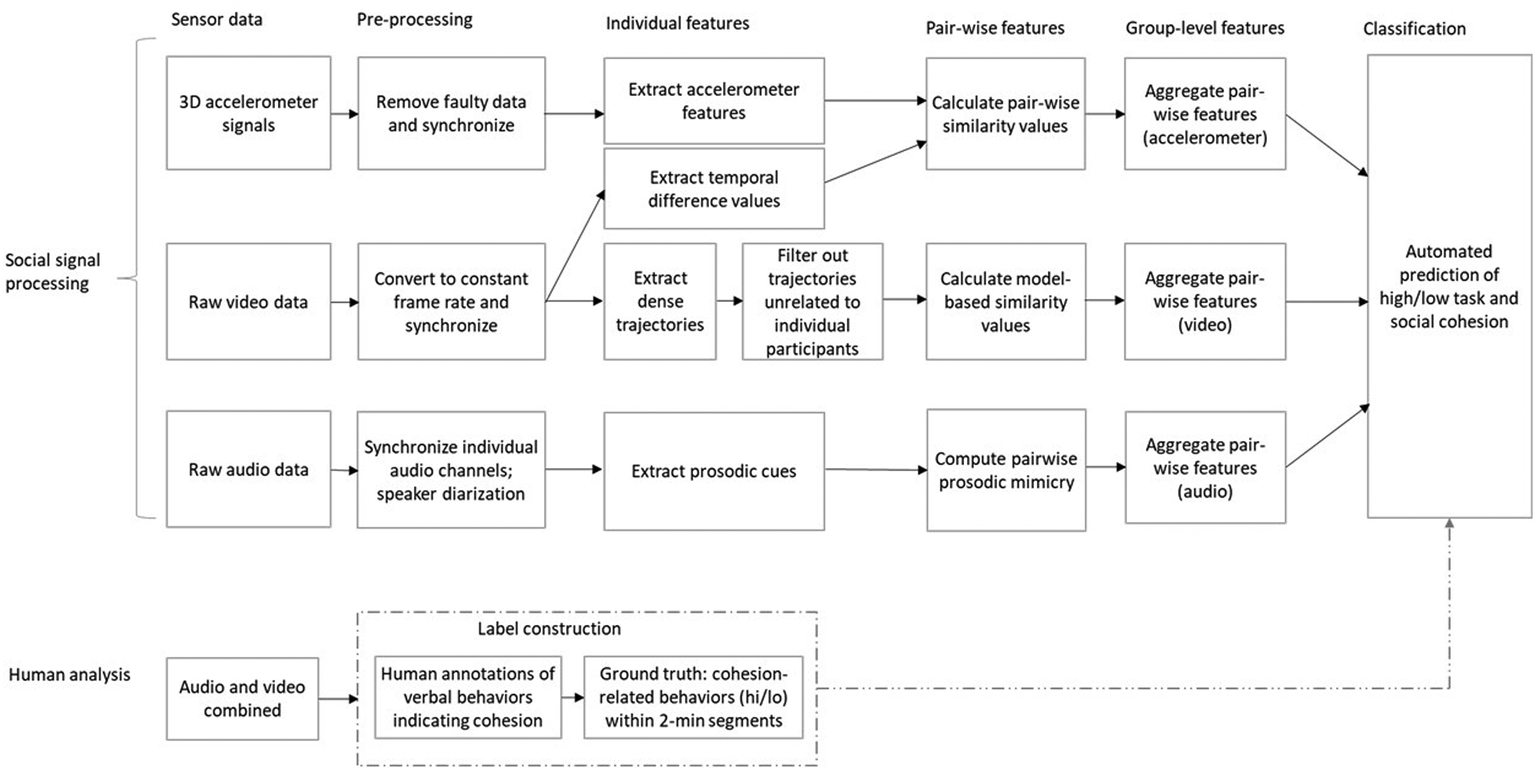
Flow chart of the work process for automatically detecting cohesion in meetings using a social signal processing approach.
Figure 3 also indicates key differences between social signal processing and the state of the art in quantitative team interaction analysis. The latter is sketched at the bottom of Figure 3 and essentially requires two steps: (1) gather behavioral team data and (2) spot behaviors of interest using trained human annotators (for more detail, see Keyton, 2018; Lehmann-Willenbrock & Allen, 2018). This means that the temporal windows for analyzing the team interaction flow are much more coarse than in social signal processing, where the behavioral units are milliseconds or picture frames rather than seconds or minutes. Furthermore, the bottom path illustrated in Figure 3 falls short of analyzing the rich multimodal quality of behavioral interaction dynamics in teams, due to the extensive human annotation effort that would be required to address this. Finally, whereas the ultimate goal in social signal processing is to automatically obtain reliable predictions of meaningful behavior from sensor data, this automation is not possible in quantitative interaction analysis (see also Allen et al., 2017, for a detailed discussion of differences in workflows when social scientists vs. computer scientists are analyzing team interactions).
We pre-processed the sensor data from each modality per team member into time series data across 2-min segments within each meeting. For each modality, we extracted features and captured behavioral synchrony and convergence across these 2-min segments (i.e., the same timeframe that was used to establish ground truth labels; see Figure 2). For the code for our feature extraction and combination, we used a combination of Python and Matlab. While we are not permitted to openly share the code, extracted features, and the underlying raw behavioral measures given privacy concerns and legal restrictions at the organization where we gathered our field data, interested readers can contact us for more information on an individual basis.
Extracting Multimodal Features
We extracted time series data from (1) the audio data (voice intensity, fundamental frequency, speech rate, and first 12 mel frequency cepstral coefficients [MFCCs]); (2) the video data (thresholded pixel-wise difference between image frames and the Histogram of Oriented Gradient [HOG] part of the dense trajectories feature vector); and (3) the accelerometer data (absolute x, y, z, and magnitude, from which six spectral and two statistical representations, namely, mean and variance, were generated—thus, 4 × (6 + 2) features).
Extracting Vocal Features from the Audio Data
From the Microcone (see Figure 1) audio data, we obtained audio segments separated by speaker. Using the open-source program Praat, we extracted the following vocal characteristics or these segments separated by speaker: (1) voice intensity, (2) fundamental frequency, (3) speech rate, and (4) first 12 MFCCs. Voice intensity is the loudness of the voice, which is measured in decibel (dB). The fundamental frequency is a physiological parameter defined as the frequency of vibration of the vocal folds, which can be measured in cycles per second or Hertz (Hz). The fundamental frequency is closely related to voice pitch, which is our human perception of fundamental frequency. The fundamental frequency generally lies in the range of 85–155 Hz for men and approximately one octave higher for women (165–255 Hz; for children, it is around 300 Hz). The speech rate or speaking rate is the tempo, in terms of the pace at which a stretch of connected discourse is delivered by a speaker. The average speech rate in conversations is typically around 3–4 words per second. We quantified the speech rate in vowels per second, using Praat software and the procedure described by De Jong and Wempe (2009). Finally, the first 12 MFCCs describe the spectral characteristics of an audio signal, in terms of different frequency bands that are determined logarithmically. They are commonly used to describe vocal behavior as their design is inspired by sound production in the human tract. These four vocal characteristics have been found to be effective for quantifying dyadic mimicry (e.g., Bonin et al., 2013; Solanki et al., 2016).
Extracting Motion Features From the Video Data
To capture motion from the video data, we extracted the thresholded pixel-wise difference between image frames in the region where a meeting participant is seated as a baseline feature. The more pixels change in intensity over consecutive frames, the higher the body motion score. Hung and Gatica-Perez (2010) used a similar approach to measure group-level cohesion except pixel-level movement was computed directly from compressed video data. The disadvantage of such approaches is that they are not able to capture movement or the shape of movement occurring over more than two consecutive video frames. Therefore, we also extracted dense trajectories (cf., Wang et al., 2013) which try to follow pixels (a 2 × 2-pixel neighborhood) over a pre-defined number of frames of a video, with a description per trajectory of the movement and appearance of the trajectory at each frame. Dense trajectories primarily describe the motion of a pixel in a video over time. The flow of the pixels is determined using optical flow fields computed on consecutive frames of the video. Then, the position of each location of the image in the next frame is determined based on the estimated flow direction. They are dense because the representation is extracted at multiple spatial scales, leading to a dense and overcomplete representation of the movement in the scene. This representation is able to describe human movement in an extremely powerful way for machine perception tasks. The default parameters are a trajectory length of L = 15 frames (see Wang et al., 2013), computed over an N × N pixels space-time volume aligned with a trajectory. The volume is subdivided into a grid, with
From the video data, we further extracted the HOG, a feature descriptor that is commonly used for object detection in computer vision and image processing (e.g., Zhu et al., 2006). The HOG represents the gradient directions of image intensity values as a distribution. These features provide a proxy of postural appearance over detected trajectories. Trajectories are associated with each person depending on whether the starting point of the trajectory originates within a pre-defined bounding box assigned for a given individual. We use a pre-defined bounding box in the image plane which represented a rectangular region over which the features for a given individual's behavior are extracted. In practice, we would prefer to be able to identify the seated person over time automatically. However, due to the uncertainty that the person would be tracked correctly and the knowledge in any case that the participants are seated throughout the meeting, we used a pragmatic approach to identify the relevant region of interest for each participant.
Extracting Movement Features From the Accelerometer Data
Accelerometer data captures movement along three orthogonal axes X, Y, and Z. The XYZ data represent the magnitude and direction of acceleration incident on each of the X-, Y-, and Z-axis, respectively. Because there can be interpersonal differences in the amount of movement in raw accelerometer signals, we first standardized each axis using z-scores. We then used these standardized values in three ways: the z-values themselves, the absolute values, and the magnitude which combines all three axes. We therefore obtained seven different features from the accelerometer data, namely, the raw and absolute value for each axis X, Y, and Z, respectively, and the magnitude for all axes combined.
We calculated absolute values, which removes the within-axis direction. The reason for using absolute values is that sometimes the direction of the movement along a particular axis might not be relevant (e.g., distinguishing forward from backward movement or left movement and right movement might not be necessary). The magnitude takes this a step further by considering just the amount of movement to be important irrespective of any direction. It is a representation of the total amount of movement a participant made and is calculated as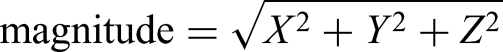
Sliding Windows
Variables such as sliding window size or sample interval length are considered parameters in the machine learning model. Using a grid search approach, one can test various values of these parameters over a range of possible values to see which yields the best results on some data used for training the machine learner while then testing the resultant tuned model on new unseen data. Our sliding window size was a parameter that was empirically validated by using a simple toy model using the accelerometer data. Both the window size and sample interval length were fixed; in this case, the sample interval length was taken from prior work which had used the same thin slice length. However, parameters related to the weights for each of the coefficients of the logistic regressor were tuned for each of the five folds of the group-k-fold cross-validation. A logistic regressor has 1 + the number of input feature dimensions (in our case 720).
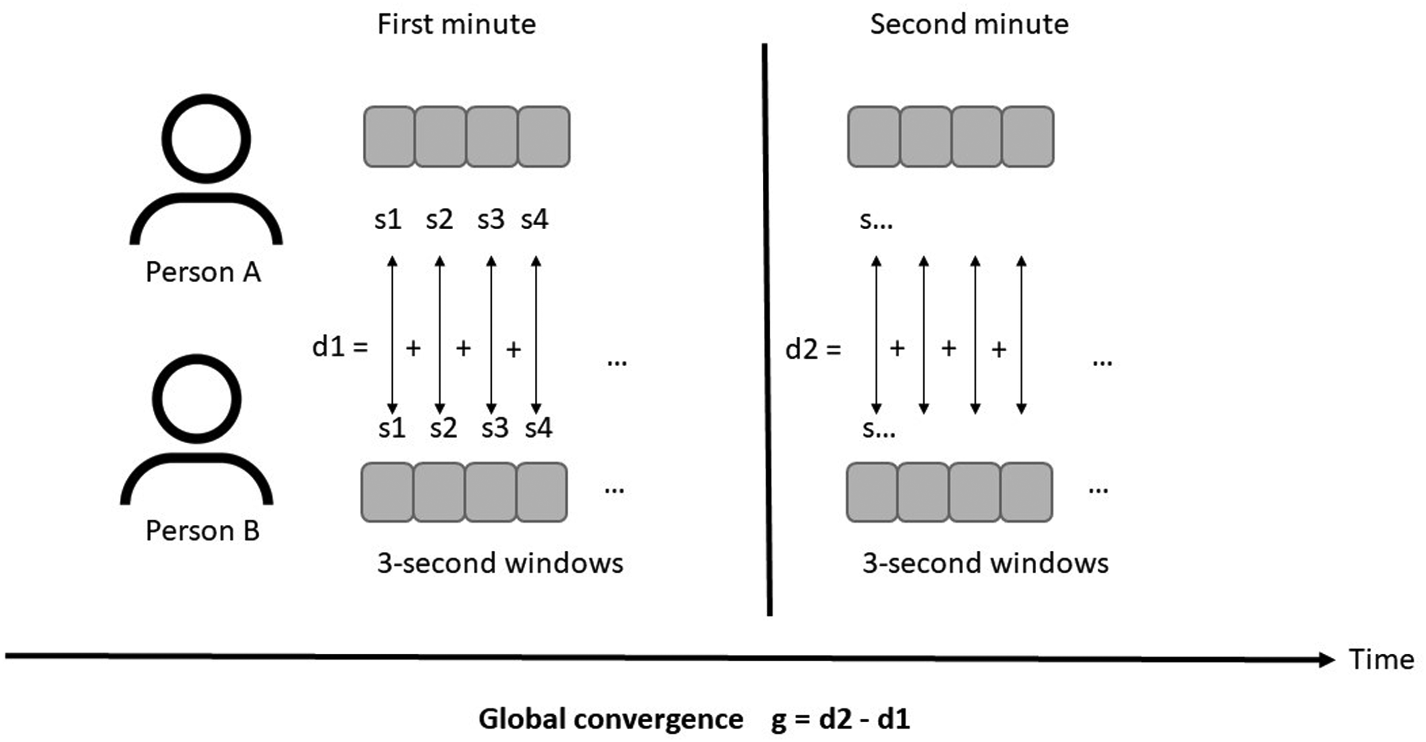
We tried sliding windows of 1, 3, 5, and 10 s (cf., Kapcak et al., 2019) and found that a 3-s sliding window yielded the best prediction performance. We compared each possible pair of participants in the team meeting using these 3-s sub-windows over the entire 2-min meeting slice (see Figure 4) and calculated the minimum, maximum, mean, and variance of the resulting differences as a representation of short-term similarity, as detailed next.
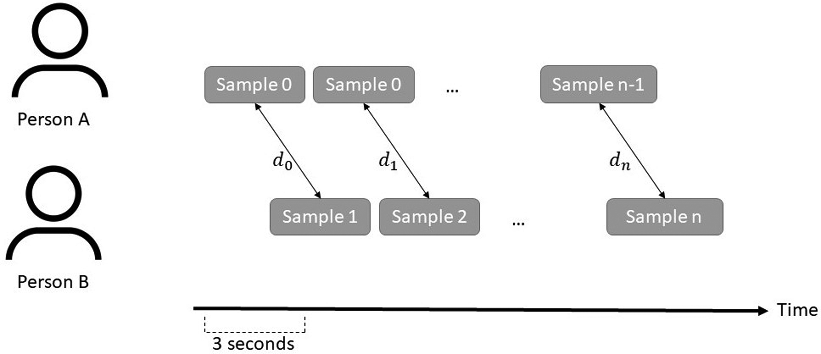
Computation of mimicry among team members. When person A is mimicking person B, they are imitating B's behavior with a delay. To measure short-term mimicry for each possible dyad in each meeting segment, we compared the two persons' consecutive 3-s sliding windows (shifting by n/2 such that consecutive windows are half overlapping, as illustrated) by calculating the distance between these windows (figure adapted from Kapcak et al., 2019). Across all of these possible comparisons within each 2-min meeting segment, we calculated the minimum, maximum, mean, and variance as a representation.
Computing Group-Level Mimicry and Convergence Features
To quantify group-level social signal mimicry and convergence for each of the included modalities, we computed group-level measures of mimicry and convergence based on measuring each person A's potential reaction to B in all possible dyads within each group. Hence, we first created pairwise similarity values for each dyad in the respective group and then aggregated these to the group level using the minimum, median, and maximum of standard deviation of the set of possible pairwise values (cf., Kapcak et al., 2019). We then added this to the feature representation by placing the set of short-term similarity features corresponding with the highest maximum first.
Mimicry of the audio features was represented by the extent to which additional data samples from one speaker followed the distributions from the other speakers in the group. We implemented model-based similarity measures for the audio signals based on Nanninga et al. (2017) to compare paralinguistic mimicry features between participants, based on the log-likelihood as follows: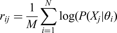
From the set of dense trajectories (see overview in Figure 3) extracted for each participant delimited by a pre-defined bounding box in the image plane, we created a model for each participant in each meeting section. We adopted a Gaussian Mixture Model to learn a compact representation of each participant's dense trajectories in order to model their synchrony and convergence with other participants in the meeting (see Nanninga et al., 2017 for a similar approach for audio data, as well as Solanki et al., 2016, for more detail on using Gaussian Mixture Models to capture social signal mimicry). By applying the features obtained from another participant on this trained Gaussian Mixture Model, we could see how well they matched the movements of a given participant in the meeting.
For the accelerometer and video-based temporal difference (TD) data, relatively few dimensions were extracted over time. We therefore used five different forms of synchrony and convergence measures: normalized mutual information, Pearson correlation, short-term similarity (i.e., mimicry), global convergence, and symmetric convergence. Normalized mutual information is calculated as 
Short-term similarity compares the difference between feature values of one meeting participant A in a given time window to those feature values of participant B in the consecutive time window (see Figure 4). Note that our measure for short-term similarity or mimicry is asymmetric, because it yields different values when comparing participant A to B versus comparing participant B to A. Because it should not matter which participant is considered as person A and which one as person B, we added the mimicry comparison with the highest maximum to the feature vector first, followed by the one with the lower maximum.
Global convergence is the difference in the behavioral features of two participants when comparing their behavior in the first half of each 2-min segment, compared to the second half of each segment (see Figure 5). Symmetric convergence is the correlation between features of person 1 and 2 in corresponding 3-s sub-windows across each 2-min segment (see Figure 6).
Calculation of the global convergence value. The distance between participants for each of the overlapping sliding windows (s) was summed for the first half of the 2-min segment as well as the second half of the segment, respectively.
Calculation of symmetric convergence, in terms of the difference between feature values of two participants for each overlapping sub-window (3 s each). The correlation between these difference values over time is the symmetric convergence rate.
From each of these, four group-level measures were created by generating the minimum, maximum, median, and standard deviation from all possible pairs for each group for a given meeting segment. This led to 5 × 4 × (4 × (6 + 2)) features for the accelerometer data and 5 × 4 × 1 features for the video-based TDs.
Synchrony was computed as the average likelihood of the samples from another participant belonging to a given person's model. Convergence was captured as pairwise similarity by computing the Pearson correlation per timestep and the likelihood. The same four group-level features were computed per pair as above, leading to 3 × 4 features for the audio and 4 × 3 × 4 features for the video-based HOGs extracted from the video data. We therefore extracted 720 features in total to train our algorithm.
Algorithm Development
Our aim was to create a machine learning algorithm that would be able to automatically detect the level of task and social cohesion (high or low) in each meeting segment, based on group-level social signal mimicry. If such an algorithm can indeed predict cohesion labels, then we can eventually use it on other datasets and avoid the hassle of laborious human annotation of team behavior. Instead, the algorithm will tell us about behavioral expressions of task and social cohesion in the observed team interactions. To get there, we needed to specify how the input from the various sensors should be processed and combined to automatically detect task and social cohesion expressions in each meeting.
In machine learning, a classifier is an algorithm that can automatically categorize data into one or more classes, such as an email classifier that scans emails and categorizes them as “spam” or “not spam.” In our case, the classes were “high task cohesion” versus “low task cohesion” and “high social cohesion” versus “low social cohesion” for each 2-min segment in each team meeting. We had two goals in our algorithm development. First, we wanted to obtain reliable predictions of task and social cohesion. Second, we wanted to be able to interpret which specific behaviors help predict task and social cohesion inside the meeting. We used a so-called simple classifier, which allowed us to look at the weights of each feature and to identify which features contribute more to successful classifications.
Specifically, we used a logistic regression model and chose a linear classifier to classify high and low cohesion using the group-level behavioral mimicry features described above. Borrowed from the field of statistics, machine learning approaches use logistic regression as a so-called supervised learning classification algorithm in order to predict the probability of a target variable (in our case, labels for high versus low task and social cohesion, respectively). If researchers want to use this approach, the nature of the dependent variable needs to be dichotomous, which means there can only be two possible classes (in our case, high or low, represented as 1 or 0 for each meeting segment). Mathematically, our logistic regression model predicts the probability of high cohesion as a function of the group-level mimicry features for each type of modality. For the multimodal version of the algorithm including all available modalities, this level of probability was averaged across the different modalities.
K-Fold Cross-Validation
Machine learning algorithm development requires training data on which the algorithm learns how to automatically detect the criterion of interest (in our case, task and social cohesion in each meeting segment) and test data for evaluating algorithm performance. To evaluate the generalizability of a proposed approach, researchers in social signal processing usually perform cross-validation. This involves partitioning the data into k folds where each fold is used to test the model while the remaining k-1 folds are used to train the parameters of the model. Each time a different fold is selected as the test fold, and then, a different model is being trained based on different training data. In our case, we also forced each fold to be stratified by group such that no data from the same group having the same meeting would appear in both the train and test folds.
Due to our field sample, we only had a limited number of meeting segment data available, particularly for training and testing the algorithm across all modalities (see Table 2). To address this, we used k-fold cross-validation and set k to 5. We divided our data into k meeting exclusive folds of which one was used as a test set and the others were used as the training set, respectively, for the machine learning algorithm. This was repeated k times so that each fold was taken as the test set once. This approach reduces over-fitting and therefore gives a more accurate estimation of performance on previously unseen data (Cawley & Talbot, 2010).
Findings
To evaluate the performance of our algorithm, we examined how well the quantified group-level mimicry within each extracted feature predicted instances of high or low task and social cohesion, respectively. Machine learning approaches measure this prediction or classification performance using metrics. In this case, due to the imbalance of the high and low cohesion samples, we used the average area under the curve (AUC) of the receiver operating characteristic (ROC) curve. The ROC curve represents the true positive rate (TPR) against the false positive rate (FPR) at different classification thresholds. Compared to other performance metrics, the AUC provides the most complete picture of how well a model is performing because the ROC on which it is based shows the performance at all possible combinations of precision and recall for the given test dataset. Appendix B provides more detail regarding reasons for selecting the AUC as a performance metric as well as how the AUC is computed, along with more information about the correlation of the different features with task and social cohesion labels across our dataset.
In addition to the AUC scores that follow, Appendix C presents different performance metrics (precision, recall, and f-measure), based on post hoc additional analyses using the extracted features. Performance metrics such as the f-measure provide an intuitive idea about model performance if the ultimate goal is to understand the efficacy of a model at the time of application. Whereas the AUC metric considers different classification thresholds, the f-measure only provides an estimate of a model's performance at a single point on the precision–recall curve. The selection of this point on the curve depends on what a user needs for a given application. If both classes (positive and negative) are considered equally important, one would choose a model threshold that maximizes both precision and recall (f1-score) jointly. However, some applications may favor higher precision and lower recall for detecting the positive over the negative class. For the interested reader, we provide results for the f-measure where precision and recall are considered equally important (see Appendix C). We caution the reader that the aim of this paper is not to provide a software tool that can be downloaded and used as is.
Comparing Feature Performance With Respect to AUC Values
The boxplot in Figure 7 shows the algorithm's classification performance for automatically detecting task cohesion (light gray) and social cohesion (dark gray) using the different features. This classification was based on the total of 720 features extracted across the entire dataset (as illustrated in Figure 2). As can be seen in Figure 7, all of the features performed better for predicting social cohesion than for task cohesion. Social cohesion was detected with an average AUC of 0.64 based on the accelerometer features, 0.63 based on the audio features, and 0.57 based on the TD features. Task cohesion was detected with a noticeably lower average AUC of 0.57 based on the accelerometer features, 0.60 based on the audio features, and 0.52 based on the TD features.
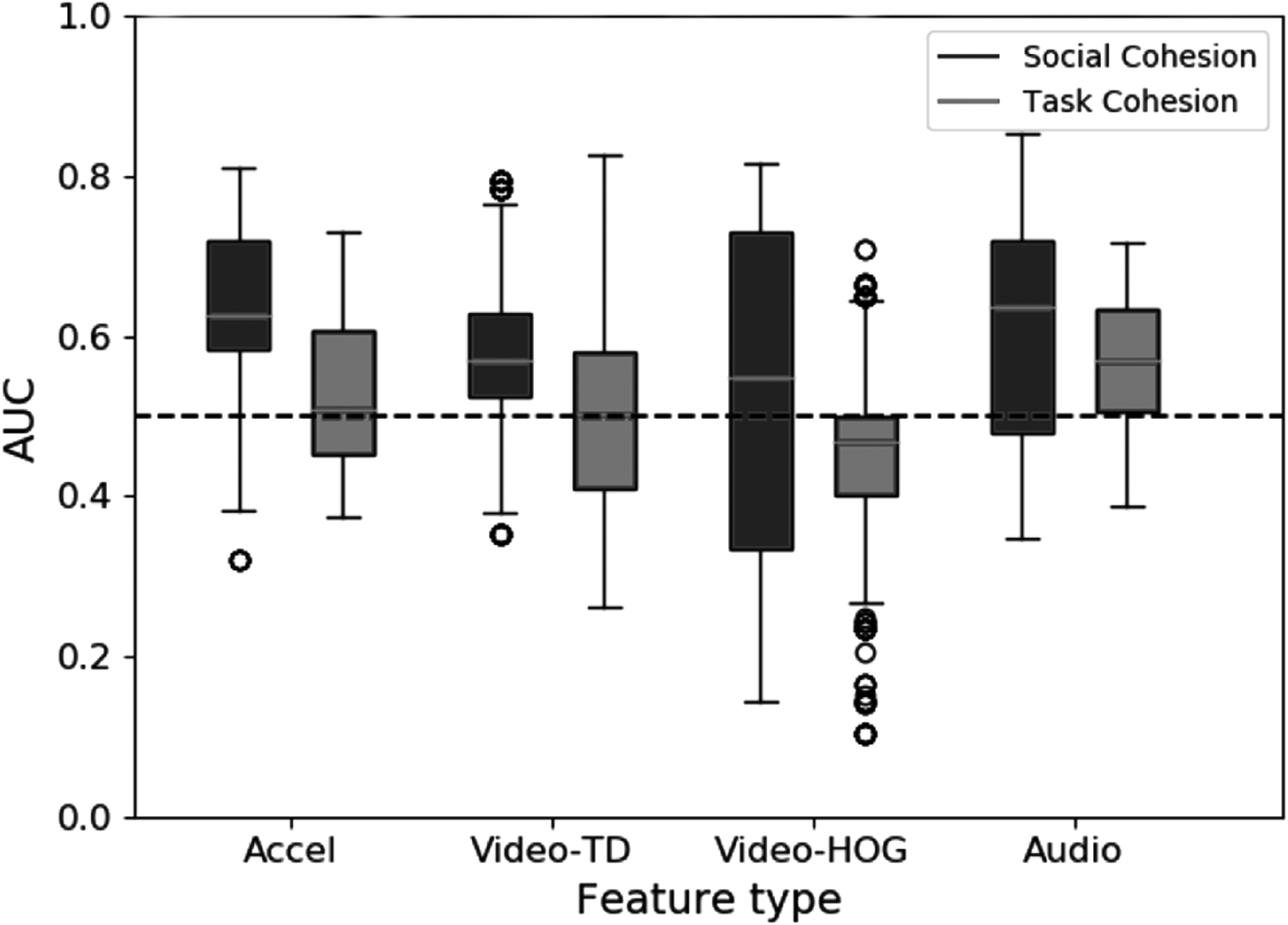
Boxplot of individual feature performance for predicting task cohesion (light gray) and social cohesion (dark gray) by each feature type, including error bars.
The reason why the audio features performed best for detecting task cohesion was likely that all team meetings had audio data, so the audio features had the largest amount of training data available (see Table 2). Because a different set of meetings was available for each modality, we cannot definitively conclude which modality detects social and task cohesion the best. Still, it appears that paralinguistic mimicry is a decent detector of both social and task cohesion, whereas motion similarity extracted from an accelerometer and TD data works for detecting social cohesion. The appearance-based HOG features seemed to detect neither.
To compare the predictive performance of the different features, we also tested the classification performance of each individual feature for the shared set (see Figure 8a). For the video features as well as the audio features, we obtained a better AUC for social cohesion than for task cohesion, respectively (see Figure 8a). Overall, the accelerometer features yielded the best performance for both social and task cohesion. Interestingly, the video TD approach captures a proxy of the speed of the movement rather than the acceleration, which may make the representation potentially more descriptive of the actual underlying behavioral process. The audio features performed poorly for detecting cohesion, compared to earlier analyses (Nanninga et al., 2017), because only a subset of our data had all modalities available for training and testing. Comparable performance was obtained when each modality was evaluated independently using all available data.
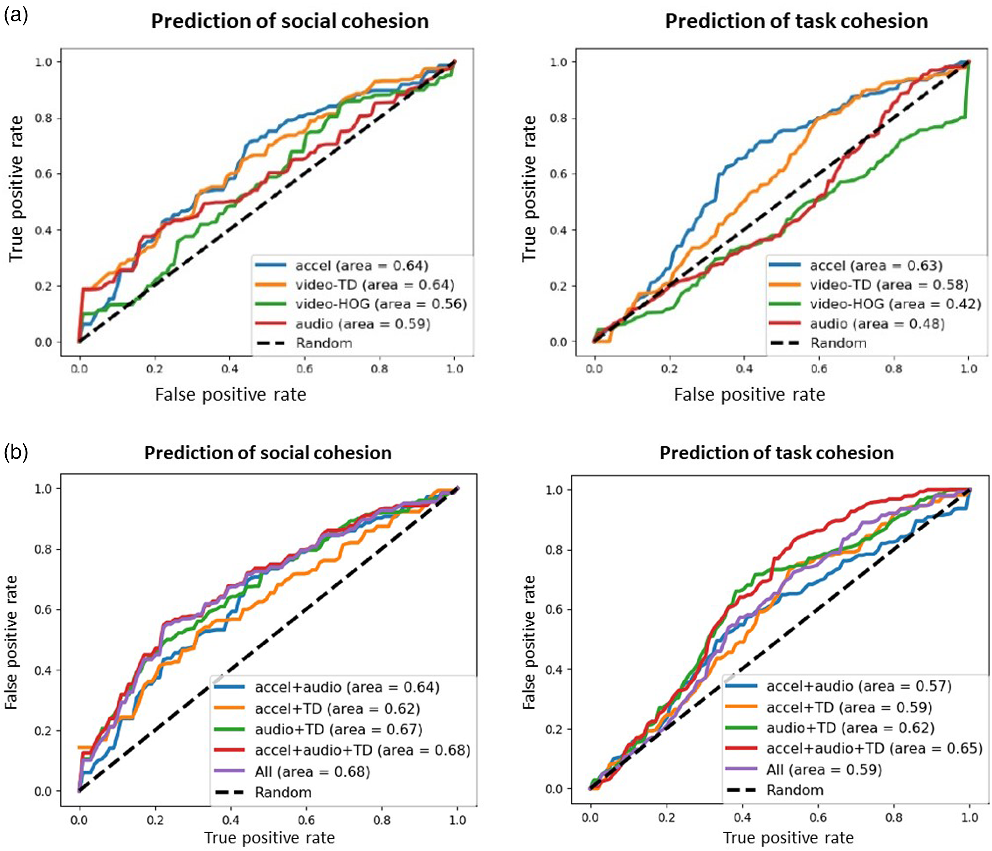
(a) Quality of the automated prediction of social cohesion (left) and task cohesion (right) by each individual feature type, as indicated by the respective average ROC curve. (b) Average ROC curve for multimodal combinations of the features in order to automatically detect social cohesion (left) and task cohesion (right), respectively.
We also examined multimodal classification performance, which means that we let the algorithm combine different features to automatically predict task and social cohesion (Figure 8b). Note that we chose not to include the HOG features in the multimodal analysis, given that these features performed poorly for predicting either type of cohesion (see Figure 8a and Appendix B for more information). As depicted in Figure 8b, the combination of audio and TD features yielded the best average performance for the two modalities, and the combination of all three modalities (video, audio, and accelerometer) yielded the highest AUC. Whereas the unimodal performance of the audio and TD video features for detecting task cohesion was not that high, the combination of audio and video led to an average AUC of 0.62. In comparison, combining the accelerometer and TD features did not improve over the performance of the accelerometer data alone—which is perhaps less surprising given that both measure movement similarity.
We obtained the best average classification performance when combining motion-based mimicry features from the accelerometer and video data with the audio features, which suggests that the combination of all different modalities does contain complementary information. However, the increase in performance was just 0.01 for social cohesion when compared to the combination of audio and TDs. Hence, while we cannot conclude that the combination of all modalities provides a significant increase in average AUC for social cohesion, the combination of features representing the two different mimicry types does seem beneficial for the detection of social cohesion. Similarly, when combining all modalities to detect task cohesion, the performance was higher compared to the detection based on accelerometer features alone, which suggests that a multimodal model detects task cohesion better than a unimodal model.
In sum, this study showcases the potential of social signal processing for automatically detecting behavioral manifestations of team constructs such as cohesion. Our findings illustrate how a multimodal approach, combining audio, movement, and video sensor data that captures mimicry at the group level, achieves the most accuracy for automatically predicting instances of social cohesion. Task cohesion was generally more difficult to predict automatically, which may partially be due to the higher overall frequency of meeting segments labeled with social cohesion compared to task cohesion behaviors in our dataset.
Discussion
Interdisciplinary work can bridge social and computer science in general and innovate methodological approaches to team interaction dynamics specifically. First, our study illustrates how a social signal processing approach can provide novel, unobtrusive measures of highly granular team interaction behaviors. To this end, we want to emphasize that automatically detecting behavioral team constructs such as cohesion still requires substantial input from social scientists in order to develop behavioral measures and establish the “ground truth” that serves as the basis for social signal processing and machine learning. In other words, as tempting as it may seem, the automated detection of team phenomena without any human annotation effort is not yet possible. To get there, more interdisciplinary collaborations between social and computer scientists are needed to create data available for computer scientists to train more robust models in “messy,” real-life team interaction settings such as the on-site project meetings investigated here.
Second, our interdisciplinary empirical approach offers a potential solution for overcoming the limitations inherent in static, survey-based measurement approaches to team constructs (e.g., Kolbe & Boos, 2019; Kozlowski & Chao, 2012; Lehmann-Willenbrock & Allen, 2018). Considering the benefits of surveys regarding the ease of data access and the low effort involved in processing and analyzing the data, compared to behavioral observations of team processes, the departure from survey-based designs can seem daunting. We hope that our study will encourage team researchers to seek out interdisciplinary collaborations that can facilitate this leap and advance our understanding of the intricate behavioral dynamics at the core of complex team phenomena such as cohesion. We suggest that team researchers should consider incorporating multiple sensors in their study design, including movement as well as audio and video data collection. The methodological setup described in our study is one example of implementing such an approach without interfering with the naturally occurring team interaction, while still obtaining multimodal behavioral data from the field.
Third, in showing how behavioral indicators of task and social cohesion in real-life team meetings are represented by the dynamics of social signals at the micro-level and across different behavioral modalities, our findings point to the importance of capturing behavioral mimicry in team interactions. Our finding that a combination of team-level movement and paralinguistic features performed best for automatically predicting behavioral team cohesion within the meeting suggests that mimicry in teams is a multimodal phenomenon. This insight speaks to calls for multimodal approaches in social signal processing more broadly (Baltrušaitis et al., 2018). An important benefit of the social signal processing approach is the ease with which multimodal behavioral phenomena can be investigated. In our case, we only looked at within-modality behavioral synchrony. Additional analyses could be carried out involving cross-modal synchrony measures, which would allow us to probe questions related to the role of inter- versus intra-modal synchrony for predicting team constructs. Furthermore, in addition to synchrony, other higher-order terms worth exploring include possible interactions between modalities (e.g., specific audio and video features might interact to predict different types of cohesion differently).
Fourth, beyond our specific example of predicting team cohesion, our findings suggest that social signal processing can be used to automatically detect complex social interaction phenomena more broadly. Indeed, computer scientists have applied social signal processing to a broad range of constructs of relevance to organizational researchers, such as detecting emergent leadership influence (e.g., Muller & Bulling, 2019), predicting group performance from social signals (e.g., Murray & Oertel, 2018), or automated analyses of group affect (e.g., Böck, 2021). Gatica-Perez and colleagues (2017) reviewed 100 social signal processing publications that focused on small group analysis and derived conversational dynamics, verticality (including dominance and leadership), team personality, and group characterization as trending topics in social signal processing that are of high relevance for organizational researchers interested in group and team dynamics, leader–follower dynamics, and social interactions at work more generally. Moving beyond the typical controlled laboratory setting in these earlier applications, our findings from real, “messy” team meetings in organizational context show that multimodal social signal processing approaches can be extended successfully to teams in the wild. As a caveat, we need to acknowledge that we are not in a position yet to fully rely on machine learning algorithms to reliably detect complex team behavior.
Our proposed approach can be easily extended to include the processing of other modalities including language, for example, by processing the transcripts generated from automatic speech recognition using pre-trained neural language embeddings. We could indeed also consider processing other information at the utterance level. However, there are privacy concerns to consider. Because we gathered field data from real project meetings, verbal transcriptions of the meetings were strictly forbidden. Given this practical constraint, it is worth considering the benefit of also developing multimodal nonverbal approaches further. This privacy-preserving aspect of our processing approach was certainly appealing to the company where we gathered the data and was a contributing factor to our collaboration with them.
Limitations and Future Research Directions
Several limitations of our approach point to future research opportunities. Some of these concern our choice of labels for dynamic cohesion. In our machine learning model, the level of cohesion was binarized. The choice to simplify the data by creating labels for high versus low task and social cohesion, rather than using continuous labels, is standard in the social signal processing community, yet this leads to a loss of detail. It remains a research challenge for the social signal processing community how to best handle these data which have neither positive nor negative classifications. One might be led to think that solving this with a regression task would be the solution. However, given the skewed nature of the data distributions as shown in Appendix A, Figure A1, computing regressions accurately remains an open problem in the field. Moreover, metrics for measuring good performance on a regressive scale tend to be harder to link back to what is actually happening in the social interaction (in our case, a meeting). This remains an open design choice for any interdisciplinary collaboration in the area of social signal processing.
Moreover, our machine learning model considered the two cohesion estimation tasks independently. In other words, all 2-min meeting segments were labeled as either task or socially cohesive, but never as both. Given that each time window within the team interaction stream could contain both utterances of task and social cohesion, each window could receive a continuous value label for the associated level of task and social cohesion present, rather than the binary categorization into high/low cohesion as applied in our case study. For instance, each behavioral unit within the team interaction would be annotated with a certain percentage of task cohesion and social cohesion. In adjusting the outputs of the estimation task and considering the problem to be one of jointly estimating task and social cohesion, other machine learning approaches such as multitask learning could be used to better predict both types of cohesion with the assumption that there is some dependency between the two phenomena that can also be learned. Notably, much more training data would be required to achieve reliable predictions on continuous labels of task and cohesion levels inside meeting segments.
Our choice of logistic regression as a supervised learning classification algorithm was one possibility among many, many others. It really remains an open question which approach would be most accurate. One of the issues to be considered in the context of our current study is that different partitions of the data would yield different results, given the type of validation approach we used due to the small sample. It would be beyond the aims and scope of this paper to compare different classifiers, but we refer the interested reader to Witten et al. (2005) for an overview of different types of algorithms and data mining methods in machine learning. Moreover, given the growing success of deep learning approaches, future research might explore machine learning approaches that learn features for social interaction from data (i.e., learned representations) rather than using prior knowledge to design features. Such deep learning approaches use artificial neural networks (e.g., Rosopa, 2022; Urban & Gates, 2021) and rely on massive amounts of data, which are far beyond the amounts available from typical samples of behavioral team interactions such as the one examined in the current study. Likewise, leveraging knowledge that can be generalized from multiple datasets, recording conditions, and contexts remains an open question. There is still a hope that with learned representations, learned models can still be adapted to a specific set of experimental data using adaptation approaches such as fine-tuning. However, future research using deep learning to detect behavioral team phenomena should aim for larger samples of in-the-wild team interactions than the one we gathered and annotated here. Moreover, we caution the reader that while deep learning approaches are powerful machine learning techniques, they fall short in terms of their interpretability. It remains an open question as to how we can resolve the semantic interpretation of such abstract representations, which can often be “in the eye of the beholder.” This phenomenon is often overlooked and can cause severe misinterpretations of machine learning results if not handled appropriately (see also Raman et al., 2022, for a discussion of this point).
In the social signal processing field, works that are showing proofs of concept tend to use simpler classifiers with feature engineering, while contributions that are more technical typically propose more robust classifiers that are designed based on hypotheses about the nature of the prediction problem. While some earlier SSP works did compare modeling with different classifiers, we deem this a rather unsatisfactory approach. This is because the explanation for why one classifier works better than the other cannot be meaningfully extracted from more complex classifiers without further analysis and often does not lead to satisfactory conclusions. This is further compounded by the comparatively small size of our field study dataset (compared to typical dataset sizes in the machine learning field). By using more sophisticated machine learning classifiers, we would reduce the model transparency and might overfit our model to unwanted nuances in the data. How to trade off these issues remains an open question for interdisciplinary research.
In the scope of modeling choices, future research could also examine to what extent data transformations may improve performance in social signal processing. Methods from generalized linear models (e.g., Rönkkö et al., 2022), such as log transformation, could potentially be applied to machine learning model performance when labels are not distributed evenly (as in the case of our labels for high and low cohesion, see Table A1 in Appendix A). Moreover, future research can investigate the potential interplay between micro-level behavioral mechanisms underlying task and social cohesion, as presently investigated, and larger-scale temporal dynamics of (emergent) task and social cohesion across longer interaction periods, such as entire meetings or series of meetings by utilizing multilevel modeling approaches.
Regarding the ground truth for variables such as cohesion at the behavioral event level, we took some liberties in our case study to establish a link between verbal utterances and labels for task and social cohesion. We provided conceptual arguments for this link, drawing from the extant literature on static measures of cohesion. Of note, we do not claim that our labels of behavioral-level cohesion are the same as overall emergent cohesion, which is typically measured using self-report surveys (e.g., Salas et al., 2015). Equating these different types of variables would be problematic, for example, because survey-type reports of a very spontaneous, subconscious coordination process such as the behavioral mimicry of social signals that represent moments of cohesion during team interactions would not be feasible. In other words, we cannot expect team members to self-report fluctuations in cohesion at the micro-level (see Mayo & Gordon, 2020). It would be like trying to ask people to annotate the mimicry while experiencing the interaction. We might label mimicry from external perceptions, but actually, we already know that these kinds of nonconscious behavioral patterns are best captured using sensors (e.g., Vinciarelli et al., 2011).
Related to our operationalization of ground truth labels for behavioral cohesion, future research can investigate questions related to construct validity when pursuing a social signal processing approach to team interactions in meetings and other dynamic social settings. Construct validity remains a potential concern regarding the work we presented here, as it pertains to the operationalization of behavioral-level team cohesion, our key phenomenon of interest and the criterion which we used to train and evaluate our machine learning algorithm. We anticipate that it will be a research challenge in and of itself to examine whether and how micro-level fluctuations in behavioral expressions of cohesion map onto team members’ self-reported experiences of team cohesion (which are prone to known biases associated with self-report methods but nevertheless insightful because they add a perceptual measurement layer; e.g., Gerpott et al., 2020). While beyond the scope of the current paper, future research can and should extend our approach to other team constructs that have not yet been operationalized at the behavioral level such that machine learning approaches can become more mainstream and more researchers can benefit from them. Moreover, future research can examine to what extent automatically detected behavioral expressions of task and social cohesion predict objective team performance outcomes, in light of previously established linkages between cohesion and performance in the survey-based literature (for an overview, see Grossman et al., 2022).
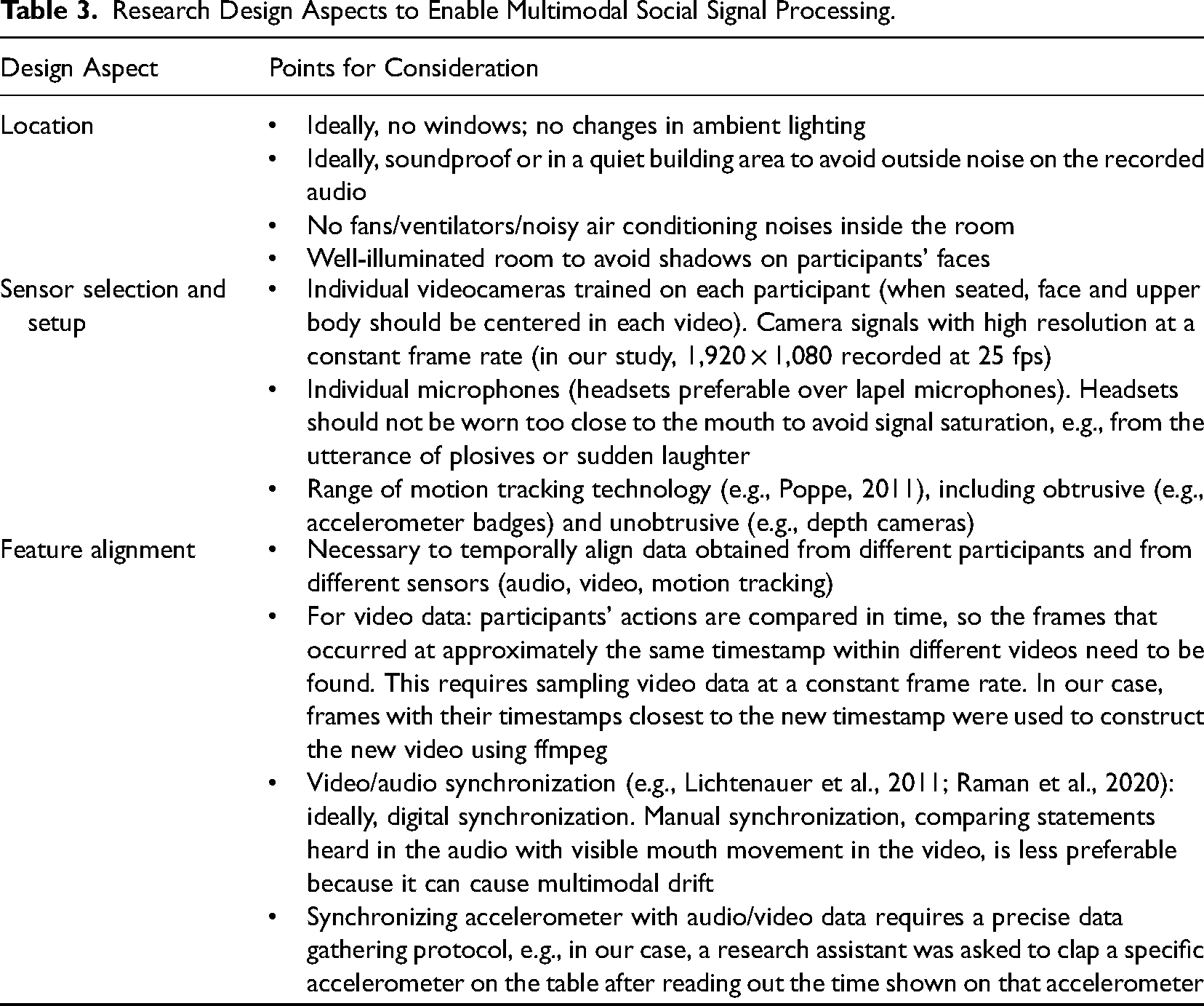
In our research example, regardless of the specific behavioral modality, the AUC score as an indicator of the quality of the automated prediction was not particularly high. Hence, the goal to replace laborious human annotations completely with artificial intelligence and rely on machine learning algorithms to tell us how teams “tick” is still a work in progress. Ideally, future work in this area will examine the performance of social signal processing approaches to group cohesion across a range of different field settings beyond the one examined in our study, thus further contributing answers to calls for more research “in the wild” voiced in both disciplines (e.g., Alameda-Pineda et al., 2018; Shuffler & Cronin, 2019). To advance interdisciplinary research in this direction, more collaborations between social scientists and computer scientists are needed. This includes the need for collaborative datasets, along with new policies and ethical procedures in place for sharing such data, and interdisciplinary foresight when designing studies (Keyton & Heylen, 2017). For researchers interested in embarking on such projects, Table 3 lists key points for consideration during research design in order to enable multimodal social signal processing.
Research Design Aspects to Enable Multimodal Social Signal Processing.
Finally, the key term “ground truth” in social signal processing warrants some reflection. For organizational researchers focusing on team processes, the idea of a “truth” can seem rather odd, given the subjectivity of team experiences and the fact that team research is not an exact science. As a side note, while machine learning researchers call the labels “ground truth,” others such as the speech processing community call them the “reference.” This accounts for the fact that the labels themselves might be subjective in some way. Historically, many traditional machine learning tasks were able to offer a more objective (true) idea of what a label should be. However, as the field has developed and more subjective phenomena are being investigated, the use of soft labels or the notion of subjectivity in the labeling process is also accepted. However, the way of modeling this subjectivity in machine learning approaches remains an open question.
To this end, scholars need to invest in developing and validating behavioral coding schemes for behavioral team constructs such as task and social cohesion. As a first step, team phenomena need to operationalize team constructs at the behavioral level such that they become observable. More scholars need to focus on team dynamics in an organizational context with methods that yield high-resolution team interaction data (e.g., Klonek et al., 2019). Organizational researchers should seek dialogue with computer scientists in order to establish data-gathering routines, including the requirements in the observational setup to gather relevant social signals at sufficient quality and enable robust multimodal social signal processing, and appropriate time windows for annotating behavioral team constructs. Alternatively, interdisciplinary research teams can explore to what extent the raw signals from sensor data can provide meaningful insights into team constructs directly. The larger question in this regard concerns the notion of representation, that is, how we may build scholarly consensus to move beyond abstract sensor information and toward meaningful social signals that represent psychological phenomena in and of themselves.
Implications for Interdisciplinary Collaboration in Social Signal Processing
Our mode of collaboration in this study can be considered a light form of the producer–consumer model (see Allen et al., 2017), where the social scientist provided the data and human annotations of the observed team interactions and advised the selection of the task and socially cohesive utterances and final interpretations of the resultant developed model. While such a lighter collaborative construction can help in the earlier phases of establishing a common ground for interdisciplinary communication, one would hope for more developed findings and outcomes moving forward with this collaboration. Looking back on the collaboration, we could have taken a more equal role with respect to the generation of joint research questions and the social scientist could have been included more in the design decisions regarding the creation of the extracted feature data. This could have perhaps led to more application-driven motivations for different machine learning models such as multitask learning or a different labeling approach based on the proportion of utterances that were task or socially cohesive within each 2-min meeting segment, as discussed above. Despite the early stage nature of this work, the joint experience has been invaluable as a common reference point to develop a joint working language for the collaboration and for furthering interdisciplinary research collaboration.
Regarding the practical implications of how such interdisciplinary work can be carried out, one of the biggest hurdles is typically related to the lack of funding, which can be a chicken-and-egg problem (i.e., without funding, no work can be carried out, and without at least preliminary work, there is typically no funding). Our experience shows that this is a common misconception and that actually low-hanging fruits do exist. While we conceptualized the research idea and study design and set up the collaboration with the organization where the data were gathered, the actual data gathering and much of the analytical work presented in this paper were then carried out by graduate students in an interdisciplinary team as part of their master theses. One format could involve one or more graduate students from each discipline working together. Beyond coordinating such an effort, this also requires that the PIs are willing to invest time in advising graduate students from the respective other discipline. As a caveat, such an approach limits the level of transdisciplinarity that the work can have since graduate students need to fulfill certain disciplinary requirements. However, such a collaboration forms a basis for establishing a common ground and language. From there, we can develop more mature co-designed research questions that can ultimately advance our conceptual understanding of social dynamics in groups and teams and computing systems that can support organizations in improving teamwork. In closing, we want to emphasize the exciting research opportunities afforded by social signal processing for innovating team science. At the same time, we are nowhere near replacing human annotators with machines in order to understand complex team phenomena such as cohesion. Continued collaboration and potentially data sharing with the wider research community will allow computer scientists to develop more robust automated machine perception approaches toward understanding more complex behavioral group and team phenomena. We hope that the growing interest in interdisciplinary initiatives in this realm (see Hung et al., 2020, for a summary) will continue to build.
Footnotes
Appendix A: Distribution of ground truth labels across the data set
Means, Standard Deviations, and Correlations of Cohesion Labels (in %) Across the Entire Data Set.
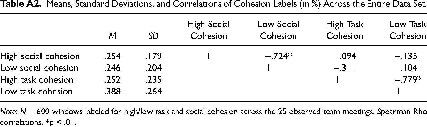
| M | SD | High Social Cohesion | Low Social Cohesion | High Task Cohesion | Low Task Cohesion | |
|---|---|---|---|---|---|---|
| High social cohesion | .254 | .179 | 1 | −.724* | .094 | −.135 |
| Low social cohesion | .246 | .204 | 1 | −.311 | .104 | |
| High task cohesion | .252 | .235 | 1 | −.779* | ||
| Low task cohesion | .388 | .264 | 1 |
Note: N = 600 windows labeled for high/low task and social cohesion across the 25 observed team meetings. Spearman Rho correlations. *p < .01.
Appendix B: AUC calculation and individual feature performance
In social signal processing, it is not customary to report a range of different performance metrics because each metric should be well motivated with respect to the sample distribution. Given the highly imbalanced class sizes in our case (see Figure A1 in Appendix A), we chose the area under the curve (AUC) as a performance metric. The AUC metric is based on the receiver operating characteristic (ROC). In machine learning, the ROC is a popular diagnostic tool for evaluation the performance of classifiers both on balanced and imbalanced binary prediction problems because “ROC analysis does not have any bias toward models that perform well on the minority class at the expense of the majority class—a property that is quite attractive when dealing with imbalanced data” (Weiss, 2013, p. 27). Compared to other performance metrics, the AUC provides the most complete picture of how well a model is performing because the ROC on which it is based shows the performance at all possible combinations of precision and recall for the given test dataset.
Appendix C: Additional calculation of different performance metrics
In addition to the preferable AUC metric (see Appendix B for a detailed justification), alternative performance metrics were requested during the revision process. As this was not anticipated, we had not saved intermediate results that would enable alternative metrics to be directly calculated from the posterior probability per sample per repeated folder. Hence, we performed a separate analysis to obtain the requested alternative performance metrics based on the extracted features and used a so-called brute force approach to identify the combination of extracted feature files that would produce results with the closest AUC to our originally generated results. As an additional verification step, we cross-checked the ROCs and AUCs with our original findings and observed a mean difference of .078 across all AUC scores, which can be attributed to expected variations in folds of the cross-validations given our random seed approach to determine the data folds during our original analysis.
Since computing the precision, recall, and f-measures forces us to discard the posterior probabilities used by the AUC and reduces them to binary classifications, an additional transformation step was necessary here. The binary prediction labels were generated by taking the highest posterior probability for each class. The results are shown in the table below, with standard deviations for all calculated metrics shown in parentheses, respectively.
Authors' Note
We appreciate the research assistance of Navin Raj Prabhu, Marjolein Nanninga, Marissa van der Wel, Sebastian Dorfmeister, Stephanie Tan, Yanxia Zhang, Dina Habib, and Fabeya Kaygun. Our field data collection was supported by Manfred Overmeen, Robert-Jan Sips, Zoltán Szlávik, and Benjamin Timmermans, which is gratefully acknowledged. An abridged version of this paper was presented as a poster at the Annual SIOP Conference 2023 in Boston.
Declaration of Conflicting Interests
The authors declared no potential conflicts of interest with respect to the research, authorship, and/or publication of this article.
Funding
The authors disclosed receipt of the following financial support for the research, authorship, and/or publication of this article: This research was partially funded by Netherlands Organization for Scientific Research (NWO) under project number 639.022.606 with associated AspasiaGrant, as well as support by IBM Netherlands.