Sage Journals: Discover world-class research

Abstract

We review the development of path model fit measures for latent variable models and highlight how they are different from global fit measures. Next, we consider findings from two published simulation articles that reach different conclusions about the effectiveness of one path model fit measure (RMSEA-P). We then report the results of a new simulation study aimed at resolving the questions of whether and how the RMSEA-P should be used by organizational researchers. These results show that the RMSEA-P and its confidence interval is very effective with multiple indicator models at identifying misspecifications across large and small sample sizes and is effective at identifying true models at moderate to large sample sizes. We conclude with recommendations for how the RMSEA-P can be incorporated along with other information into model evaluation.

Keywords

measurement models multiple regression < quantitative research quantitative: structural equation modeling

One of the most popular types of structural equation models includes latent variables assessed with multiple indicators, and these models are used to test theories proposing causal relations among the latent variables. Among the various goodness-of-fit measures used with these models, we distinguish between those which attempt to focus on the viability of proposed causal relations among latent variables, as compared to those originally developed that also incorporate information about other parts of the model (links between latent variables and their indicators, covariances among exogenous variables). We will refer to this newer class of fit measures as path-related, to reflect their focus on “relationships of dependency- usually accepted to be in some sense causal- between the latent variables” (McDonald & Ho, 2002, p. 65). Alternatively, those indices that reflect the entire model are commonly referred to as global fit indices, with two current recommended examples being the CFI (Bentler, 1990) and the RMSEA (Steiger & Lind, 1980).

McDonald and Ho (2002) linked their interest in path model fit to the popular global fit measure RMSEA developed by Steiger and Lind (1980) and Steiger (1989). The RMSEA has been described by Browne and Cudeck (1993) as a “measure of discrepancy per degree of freedom of a model” (p. 144). McDonald and Ho (2002) were the first to empirically investigate path model fit vs. global fit, as they conducted re-analyses to obtain RMSEA path model fit values using published results from 14 studies from top psychology journals. The distinction between global and path model fit raised by McDonald and Ho was subsequently pursued within the organizational research community. Williams and O’Boyle (2011) and O’Boyle and Williams (2011) added the “-P” to the RMSEA label to avoid confusion while referring to the RMSEA of the path model as proposed by McDonald and Ho (2002) as compared to the global composite model.¹ More recently, Williams, O’Boyle, and Yu (2020) examined articles from six top management journals for the 2001–2014 time period. Their findings replicated those of McDonald and Ho (2002) and show that evidence of good global fit can be obtained even if the path part of a latent variable model is misspecified, raising questions about conclusions reached by organizational researchers using global fit values. While the results above comparing global vs. path model fit with sample data are provocative, the accuracy of their conclusions requires that the RMSEA-P is effective at distinguishing between correctly specified and misspecified models. Available evidence is conflicting about such effectiveness, and the present study attempts to resolve these conflicting conclusions about the RMSEA-P. We will attempt to determine if the RMSEA-P can be effectively used to distinguish between correct and incorrectly specified path models, identify conditions when it is most effective, and discuss its use in the broader context of model evaluation.

Although first recommended by McDonald and Ho in 2002, the RMSEA-P was not evaluated via simulation until Williams and O’Boyle (2011) conducted a study based on models taken from representative SEM research (see Figure 1). Williams and O’Boyle used previously published simulation-based mean chi-square and degrees of freedom values (Williams & Holahan, 1994) to calculate mean RMSEA-P point estimates and related confidence intervals for true models and misspecified models in which true paths were omitted. In evaluating their results, Williams and O’Boyle (2011) used existing RMSEA guidelines that values less than 0.05 indicate a model with close approximate fit, values between .05 and .08 indicate reasonable fit, with values between .08 and .10 indicate mediocre fit, and higher values indicate unacceptable fit of the model. As for the RMSEA-P confidence intervals, they also followed traditional guidelines for the RMSEA and recommended a path model would be rejected if the lower bound of the confidence interval was greater than .05 or if the upper bound was greater than .10. For the present paper, we will refer to the combined use of RMSEA-P point-estimates and confidence intervals as just described as the PECI approach, to distinguish it from use of only the point-estimate (PE approach) in model evaluation.

Figure 1.
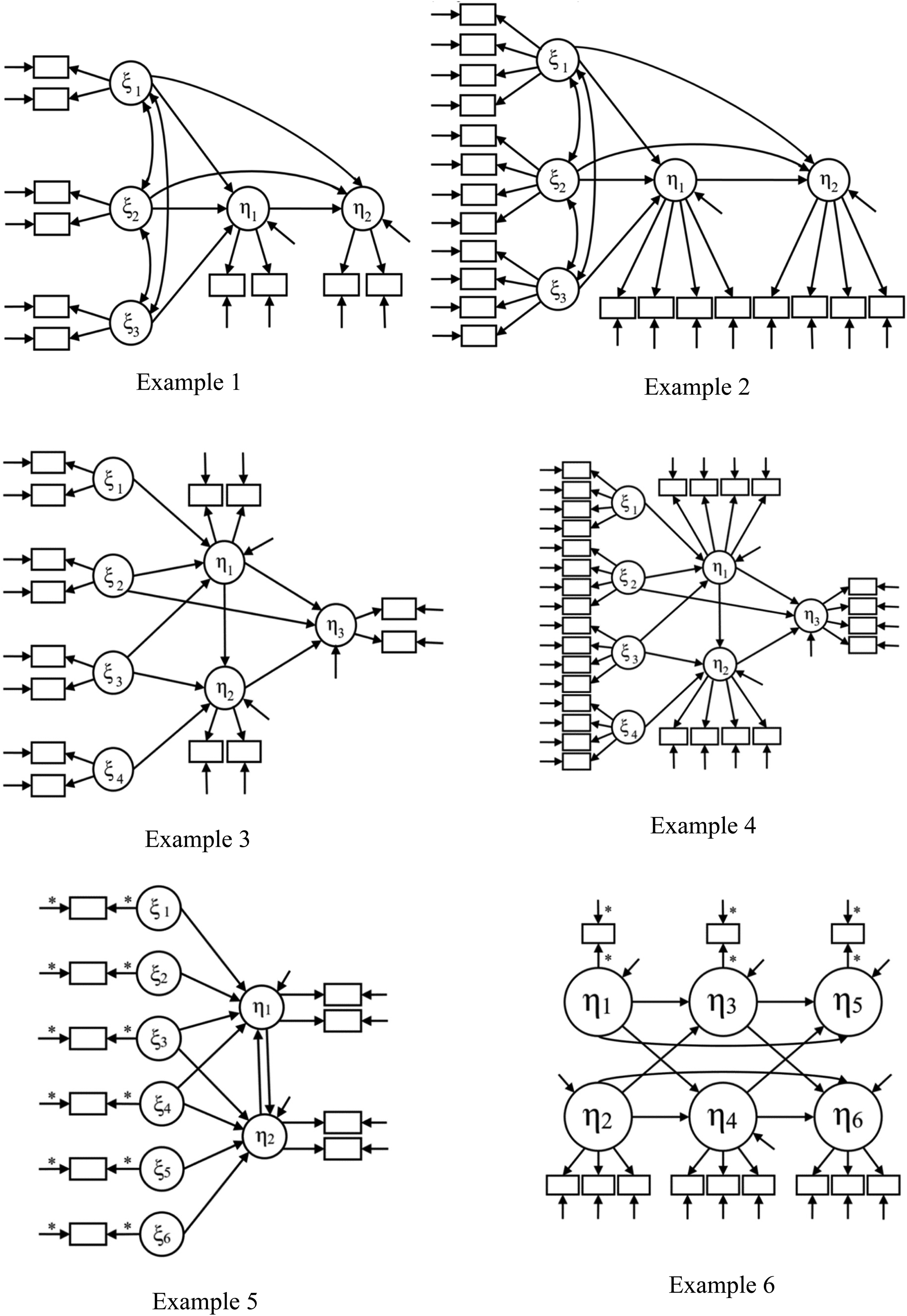
M_t for six examples.

Williams and O’Boyle (2011) found with their simulation that the RMSEA-P with the PECI approach performed as desired in five of the six examples studied with a single sample size of 500. For these five examples, all misspecified models had mean RMSEA-P values greater than .08, with mean lower bound confidence intervals greater than .05 and higher bounds greater than .10. Across the five examples, all true models (M_T) had mean values less than the .08 cut-off value often used, and all also met confidence interval requirements of lower bound less than .05 and upper bound less than .10. Results were less supportive with a sixth example. For this example, while the RMSEA-P performed as desired by correctly identifying M_T, Williams and O’Boyle found that models with one or two true paths left out (M_T−1, M_T−2) had mean RMSEA-P values less than .08 and the high end of the interval less than .10.

More recently, Lance, Beck, Fan, and Carter (2016) reached a less favorable conclusion about the RMSEA-P based on their own simulation study. They used the same six population SEM models used by Williams and O’Boyle (2011) but with the added step that they generated individual sample data sets. In presenting their findings, in their Table 11, Lance et al. only reported summaries of the frequency across individual samples that true and misspecified models yielded satisfactory RMSEA-P values (point estimates <.08) that would lead to these models being retained rather than rejected. Specifically, Lance et al. used the PE approach and summarized their RMSEA-P findings by combining across the six examples, while separating results based on four sample sizes (100, 200, 500, 1000). Especially noteworthy is that Lance et al. reported that use of RMSEA-P point estimates led to retention and support of models with key misspecifications: models with one or three significant paths omitted would have been inappropriately retained in over 50% of their simulated samples. For example, their results showed that even for a severely misspecified model with three true paths omitted (M_T−3), RMSEA-P values less than .08 were obtained in 42%–54% of cases, as the sample sizes increased from 100 to 1000. Additionally, their findings indicated that the correct model M_T frequently had RMSEA-P values greater than the desired .08, which would lead to their rejection. Specifically, Lance et al. reported this occurred in from 35% to 46% of cases as sample sizes increased from 100 to 1000. The negative assessment of the RMSEA-P by Lance et al., who based on their results recommend it never be used, is quite different from Williams and O’Boyle (2011), who suggested that it be used except when latent variables have very few indicators.

We now describe four important characteristics of both studies that make comparing their findings and judging RMSEA-P effectiveness difficult. First, Lance et al. (2016) did not provide any specific descriptive information about their RMSEA-P results, such as mean RMSEA-P values and confidence intervals. Instead, they only summarized the frequency of obtained RMSEA-P values less than .08 for the various design conditions. Not a single RMSEA-P value was reported that could be compared to any of those from Williams and O’Boyle (2011). Second, Lance et al. combined results across all six examples in reporting these frequencies, and as a result, it cannot be determined whether the RMSEA-P performed differently in all six examples. This limitation is important because in the original simulation study by Williams and O’Boyle (2011), the RMSEA-P performed well in five of the six examples. Since the design of Lance et al. was the same as the one that generated the findings of Williams and O’Boyle (2011), it seems possible, if not likely, that many of the non-supportive findings of Lance et al. may be concentrated in only a small subset of the six examples. Third, Lance et al. did not supplement their use of point-estimates of the RMSEA-P with confidence intervals (unlike Williams and O’Boyle who used the PECI approach with mean values). In other words, they used the PE approach rather than the recommended PECI approach. As a result, some of the misspecified models retained by Lance et al. based on RMSEA-P point-estimates less than the .08 cut-off value may have been rejected had confidence interval results been examined. This would occur for cases with upper bound confidence interval values greater than .10.

Fourth, Williams and O’Boyle (2011) were limited to using previously published mean-level data based on the single sample size of 500 in computing their RMSEA-P and confidence interval values (in contrast to Lance et al.'s examination of individual sample results based on use of four sample sizes). These features of their design limit the generalizability of their results. To illustrate why individual sample results are important, consider that a model with a mean RMSEA-P value of .11 (which would be seen unfavorably using the criteria of .08) would have some individual samples in which the sample estimate was less than .08 leading to the model being retained using the PE approach. And, a model with a mean value less than .08 might have some samples for which the upper confidence interval limit is greater than .10, leading to its rejection using the PECI approach. Furthermore, the sample size used by Williams and O’Boyle (2011) is larger than that of typical micro-organizational research. Thus, the findings of Williams and O’Boyle (2011) may not fully indicate the degree to which researchers can reliably identify true and misspecified models in their individual samples with typical sample sizes.

The persistent and growing popularity of structural equation models, coupled with the awareness that global fit indices can mask significant misfit within the model component linking latent variables, results in a need for path model fit indices that accurately identify correct and incorrectly specified models. However, as described above, organizational researchers using latent variable models are presented with conflicting evidence about the effectiveness of one path model index, the RMSEA-P. Given the importance of evidence of correct model specification for subsequent interpretation of parameter estimates linking latent variables, there is a clear need to reconcile the disparate conclusions in order to determine the true viability of the RMSEA-P. The present study attempts to respond to this need.

Method

Inn the present study, we use the same six example models used by both Williams and O’Boyle (2011) and Lance et al. (2016) to evaluate RMSEA-P effectiveness. Our desire was to incorporate features from both designs used in these studies and obtain results that would allow for a understanding and resolution of the differences in conclusions between the two studies. Towards that end, it was noted that Lance et al. did not report any RMSEA-P values in their results. However, they did provide the mean chi-square values for each theoretical model (correct and misspecified) and their corresponding saturated structural model (confirmatory factor analysis model). They reported this information separately for each of the six substantive examples provided and each of the four sample sizes simulated (100, 200, 500, 1000). We used their mean chi-square values and associated degrees of freedom to compute a population path model chi-square difference value $(χ_{P}^{2} = χ_{T}^{2} - χ_{S S}^{2})$ and difference in degrees of freedom value (df_P = df_T−df_SS) for each of the combinations of examples, models, and sample sizes. These computed values became the basis of our data generation process. In following this process, our goal was to use information reported by Lance et al. to generate RMSEA-P values that would allow us to replicate their Table 11 results, while further allowing us to investigate differences between samples and implications of using confidence intervals to supplement point-estimates.

For each combination, we used the χ²_P and df_P as population values, and we generated 1000 random sample χ²_P values assuming a non-central chi-square distribution.² Based on the noncentrality parameter λ for the path model as χ²_P−df_P, the mean of the generated distribution for each combination was set at df_P + λ and the variance was set at 2(df_P + 2 λ). We then used these simulation-generated sample χ²_P to compute the $RMSEA - P = {[χ_{P}^{2} – d f_{P}] / [d f_{P} * (N - 1)]}^{1 / 2}$ and its associated confidence interval for each of the 1000 replication values in each cell (representing a particular combination of example, model, and sample size). For each cell of the design, we next determined the number of models across all random samples (out of 1000) that would be retained based on both the PE and PECI approaches. We emphasize that although our method of obtaining χ²_P values is different from Lance et al., we will show that our resulting RMSEA-P values correspond to what would have been obtained had we generated individual data sets with chi-square values as was done by Lance et al. and Williams and O’Boyle (2011).

Results

To check the accuracy of our simulated data, we examined the means and standard deviations of our sample χ²_P values and confirmed they matched the population values based on Lance et al. (2016) we used to generate our data. We also used results reported by Lance et al. (2016, Tables 2–7) to compute mean RMSEA-P point estimate and confidence intervals based on their data using their published mean chi-square, degrees of freedom, and sample sizes.³ We compared these computed values to corresponding RMSEA-P results from our data (mean values of each cell for its 1000 cases). The two sets of RMSEA-P values were nearly identical across the 72 combinations of models, indicating our data was generated appropriately and that further comparisons of our results with those of Lance et al. were warranted. In other words, the similarity of RMSEA-P values indicates our results are the same as if we had generated the raw data for models and used their chi-square values to compute RMSEA-P values.

Table 2.
Results for Example 2 (MacCallum, 1986, 4-indicators).

Model N χ²_P df_P Mean RMSEA-P Mean RMSEA-P Lower bound CI Mean RMSEA-P Upper bound CI # of cases PE retain # of cases PECI retain

SN 100 297.178 7 0.646 0.582 0.708 0 0

SN 200 585.300 7 0.644 0.599 0.687 0 0

SN 500 1457.740 7 0.644 0.616 0.672 0 0

SN 1000 2912.920 7 0.645 0.625 0.664 0 0

T-3 100 92.534 4 0.470 0.383 0.551 0 0

T-3 200 183.040 4 0.473 0.413 0.530 0 0

T-3 500 452.239 4 0.473 0.436 0.510 0 0

T-3 1000 894.610 4 0.472 0.446 0.498 0 0

T-1 100 37.783 2 0.419 0.291 0.532 0 0

T-1 200 73.078 2 0.419 0.333 0.499 0 0

T-1 500 182.141 2 0.424 0.370 0.475 0 0

T-1 1000 358.836 2 0.422 0.385 0.458 0 0

T 100 1.141 1 0.040 0.001 0.199 775 0

T 200 1.078 1 0.026 0.000 0.139 862 0

T 500 1.005 1 0.015 0.000 0.087 955 805

T 1000 1.024 1 0.011 0.000 0.061 992 950

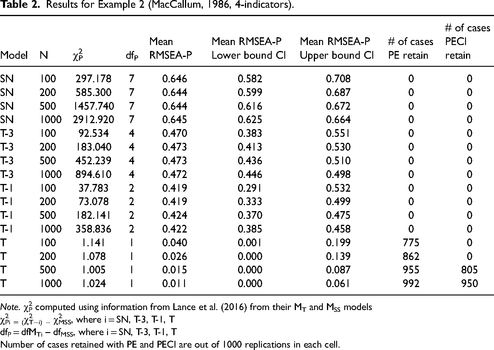
Note. χ²_P computed using information from Lance et al. (2016) from their M_T and M_SS models

χ²_{Pi = (}χ²_{T−i) −} χ²_MSS, where i = SN, T-3, T-1, T

df_P = dfM_Ti – df_MSS, where i = SN, T-3, T-1, T

Number of cases retained with PE and PECI are out of 1000 replications in each cell.

Example 1. Path diagrams for the true model M_T for all six examples are provided in Figure 1. The first example involves the use of a mediation model originally used by MacCallum (1986) that has three correlated exogenous latent variables impacting a mediator variable, which then influences an outcome variable. There are two of three possible direct paths from the exogenous latent variables to the outcome variables included in the model, and it was first examined using two indicators per latent variable. The results in Table 1 with our simulated data show that for this example, the RMSEA-P performs as desired for identifying misspecified models. Specifically, all misspecified models had RMSEA-P mean values greater than .08, all lower bounds of CI were >.05 and all higher bounds were >.10. Even for M_T−1, with only a single true path omitted, results clearly identified it as misspecified, in that across the four sample sizes, RMSEA-P means ranged from .407 to .417, low ends of CI ranged from .279 to .379, and high ends ranged from .453 to .520. More importantly, at the case level as shown in Table 1, the application of the PE and PECI approaches and criteria resulted in all misspecified models being appropriately rejected in all of the individual samples. Specifically, in all of these instances, there were zero cases where a misspecified model had a point estimate less than .08, a lower bound of the confidence interval less than .05, and a high bound less than .10.

Table 1.
Results for Example 1 (MacCallum, 1986, 2-indicators).

Model N χ²_P df_P Mean RMSEA-P Mean RMSEA-P Lower bound CI Mean RMSEA-P Upper bound CI # of cases PE retain # of cases PECI retain

SN 100 295.916 7 0.645 0.58 0.706 0 0

SN 200 588.079 7 0.645 0.601 0.689 0 0

SN 500 1458.702 7 0.644 0.616 0.672 0 0

SN 1000 2912.538 7 0.644 0.625 0.664 0 0

T-3 100 85.729 4 0.451 0.364 0.532 0 0

T-3 200 171.560 4 0.457 0.397 0.515 0 0

T-3 500 427.296 4 0.46 0.423 0.496 0 0

T-3 1000 848.161 4 0.459 0.433 0.485 0 0

T-1 100 35.965 2 0.407 0.279 0.52 0 0

T-1 200 72.034 2 0.416 0.33 0.497 0 0

T-1 500 176.576 2 0.417 0.364 0.468 0 0

T-1 1000 350.419 2 0.417 0.379 0.453 0 0

T 100 1.017 1 0.036 0 0.195 784 0

T 200 0.991 1 0.024 0 0.137 870 0

T 500 1.087 1 0.017 0 0.088 943 780

T 1000 0.998 1 0.011 0 0.061 992 950

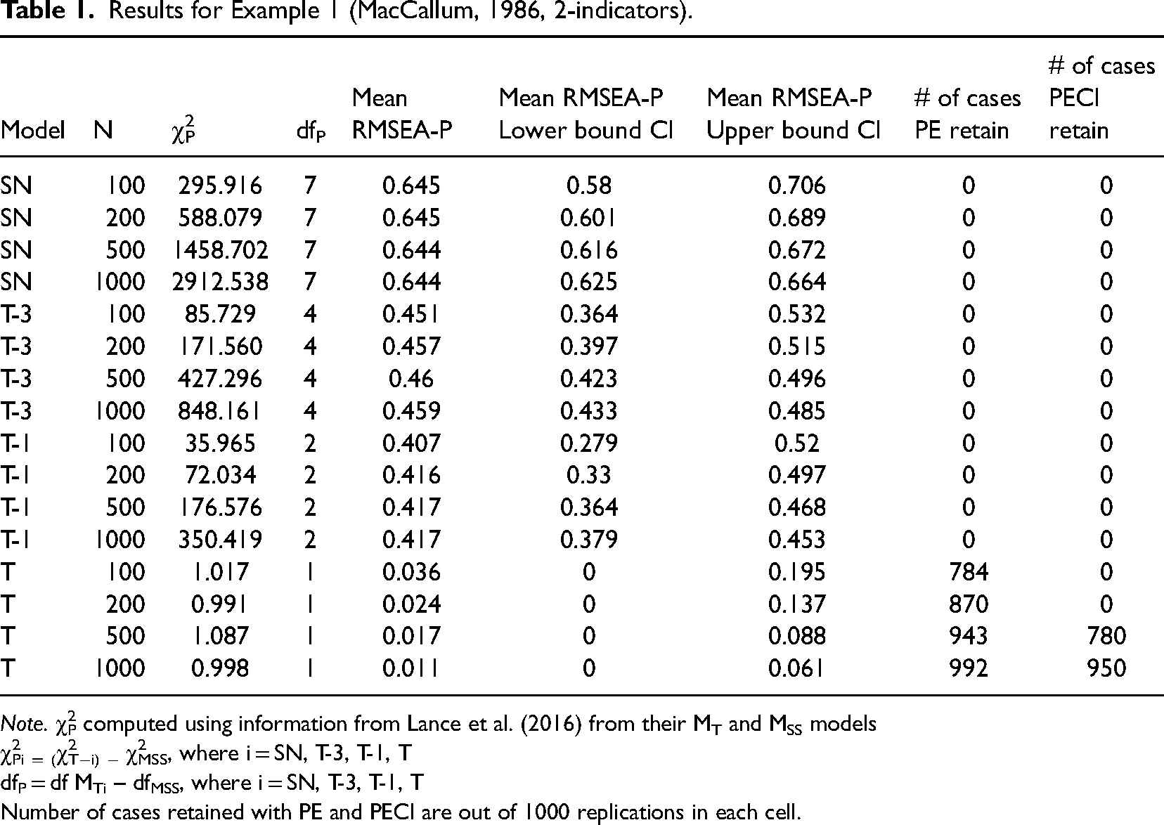
Note. χ²_P computed using information from Lance et al. (2016) from their M_T and M_SS models

χ²_{Pi = (}χ²_{T−i) −} χ²_MSS, where i = SN, T-3, T-1, T

df_P = df M_Ti – df_MSS, where i = SN, T-3, T-1, T

Number of cases retained with PE and PECI are out of 1000 replications in each cell.

For the true model M_T, the RMSEA-P mean values were acceptable (<.08) across all sample sizes, ranging from .011 to .036. However, for the two smaller sample sizes (n = 100, 200), the mean values of the high end of the CIs were > .10 (.195, .137), indicating for these cases the model would be rejected. For the two larger sample sizes (n = 500, 1000) the upper bound mean was <.10 (.088, .061). At the case level, the use of the PE criteria resulted in M_T being correctly identified as the true model with increasing frequency as the sample size increased (from 784 to 992). In contrast, the PECI approach resulted in M_T being retained in no cases for the two smaller sample sizes, but it was correctly identified in 780 of the 1000 cases when n = 500 and in 950 cases when n = 1000.

Example 2. This example is also based on MacCallum (1986), only while the latent variable structure was the same, each latent variable was measured using four indicators (rather than two). The results in Table 2 show a similar pattern as Example 1, in that across all four sample sizes for all misspecified models, the RMSEA-P had mean values indicating rejection (>.08), and the lower and upper bound CI values were greater than .05 and .10, respectively. For instance, with Example 2, we found that for M_T−1, the mean RMSEA-P values ranged from .419 to .424, the mean lower bounds of the confidence intervals ranged from .291 to .385, and the mean upper bounds ranged from .458 to .532. These and other RMSEA-P values for Example 2 were very similar to those based on Example 1, which was based on use of two indicators for the latent variables. And as with Example 1, at the case level, use of the PE and PECI approaches with individual samples resulted in no misspecified models being retained.

For M_T, the results also parallel those from the two-indicator version in Example 1, in that the RMSEA-P mean values were acceptable for all four sample sizes. The upper-end CI mean values were >.10 with the two smaller sample sizes. And, as with Example 1, for the two larger sample sizes, the mean upper-end CI values were less than .10 (.061, .087), supporting retaining the true model. Results from individual samples and the use of the PECI approach also followed those of Example 1, in that as sample size increased, it was more likely the true model would be correctly retained (from 775 to 992 cases as n increased from 100 to 1000). And like Example 1, with the two smaller sample sizes, there were no cases where use of the PECI approach resulted in retention of M_T, while in 805 and 950 instances, M_T was correctly identified with the two larger sample sizes.

Examples 3 and 4. These two examples were based on Mulaik et al. (1989) and include four correlated exogenous variables impacting two mediator variables, both of which impact an outcome variable. It is a partially mediated model, and the four exogenous variables have different patterns of relationships with the mediators and the outcome. The results based on two indicators per latent variable, Example 3, are presented in Table 3, and conclusions are the same as for the first two examples: all misspecified models had mean RMSEA-P values >.08, lower bounds of CI were >.05, and upper bounds were >.10. Thus, all would be correctly rejected. As an example, for M_T−1 the RMSEA-P had mean values across the four sample sizes ranging from .218 to .222, lower bound means ranged from .145 to .202, and upper bound means ranged from .241 to .280. Regarding individual cases, with the PE approach, there were two instances of a misspecified model being incorrectly retained when one path was omitted with the smallest sample size; in all other cases, these models were rejected based on having point-estimates less than .08. More importantly, also matching results from Examples 1 and 2 use of the PECI resulted in no misspecified models being retained.

Table 3.
Results for Example 3 (Mulaik, 1986, 2-indicators).

Model N χ²_P df_P Mean RMSEA-P Mean RMSEA-P Lower bound CI Mean RMSEA-P Upper bound CI # of cases PE retain # of cases PECI retain

SN 100 443.985 15 0.537 0.493 0.579 0 0

SN 200 870.240 15 0.535 0.504 0.565 0 0

SN 500 2171.066 15 0.536 0.517 0.555 0 0

SN 1000 4327.023 15 0.536 0.523 0.5 0 0

T-3 100 124.062 9 0.358 0.299 0.412 0 0

T-3 200 242.230 9 0.360 0.320 0.399 0 0

T-3 500 595.679 9 0.361 0.336 0.385 0 0

T-3 1000 1189.235 9 0.362 0.345 0.379 0 0

T-1 100 41.185 7 0.218 0.145 0.280 2 0

T-1 200 74.658 7 0.219 0.171 0.262 0 0

T-1 500 179.369 7 0.221 0.193 0.249 0 0

T-1 1000 352.468 7 0.222 0.202 0.241 0 0

T 100 6.690 6 0.035 0.001 0.125 822 0

T 200 6.192 6 0.021 0.001 0.086 960 797

T 500 6.084 6 0.013 0.000 0.054 1000 999

T 1000 5.893 6 0.009 0.000 0.038 1000 1000

T + 1 100 5.622 5 0.036 0.001 0.132 786 0

T + 1 200 5.323 5 0.023 0.001 0.091 940 743

T + 1 500 5.075 5 0.013 0.000 0.057 1000 994

T + 1 1000 5.011 5 0.009 0.000 0.040 1000 1000

T + 3 100 3.260 3 0.036 0.001 0.150 782 0

T + 3 200 3.185 3 0.025 0.001 0.105 902 656

T + 3 500 3.068 3 0.014 0.000 0.066 998 954

T + 3 1000 3.228 3 0.011 0.000 0.047 1000 999

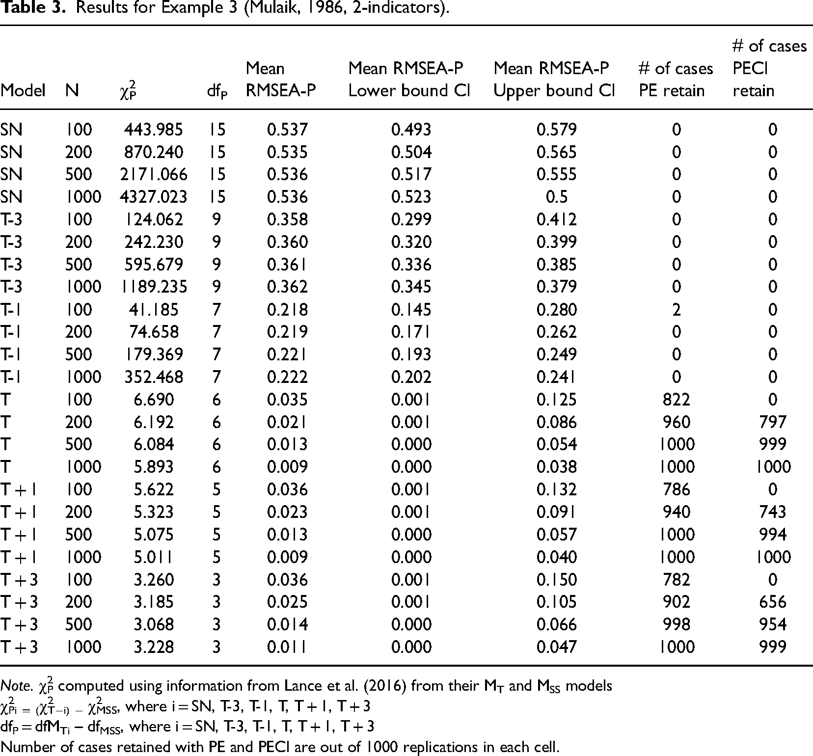
Note. χ²_P computed using information from Lance et al. (2016) from their M_T and M_SS models

χ²_{Pi = (}χ²_{T−i) −} χ²_MSS, where i = SN, T-3, T-1, T, T + 1, T + 3

df_P = dfM_Ti – df_MSS, where i = SN, T-3, T-1, T, T + 1, T + 3

Number of cases retained with PE and PECI are out of 1000 replications in each cell.

For M_T, the findings indicate mean RMSEA-P values below .08 for all four sample sizes (ranging from .009 to .035). For M_T confidence intervals, similar sample size effects were obtained as in the other three examples. The lower bound CI values showed that as before, for n = 100 the mean upper bound was >.10 (.125), while the results were favorable for the three larger sample sizes (high end values <.10). At the case level, use of the PE resulted in the number of true models being appropriately retained increasing as sample size increases, from 822 to 1000. Use of the PECI resulted in no cases of retention with n = 100, but correct retention of M_T for from 797 to 1000 as sample size increased from 200 to 1000.

When four indicators were used instead of two (Example 4, Table 4), the mean RMSEA-P values and the CI values matched the results with two indicators. With Example 4, for M_T−1 and all other misspecified models, results show these incorrect models were correctly rejected based on the PE and PECI approaches, while M_T would have been correctly retained with the three larger sample sizes (for n = 100, mean upper end values was .122). Application of the PE with individual cases resulted in correct identification of M_T from 836 to 1000 cases across all four sample sizes. The PECI resulted in no retention of M_T with the smallest sample size, while the PECI approach resulted in the correct model being retained an increasing number of times, from 801 to 1000 across the three largest sample sizes. In combination, across the first four examples, the RMSEA-P used with the PECI approach at the case level was 100% successful at identifying misspecified models. For M_T, with the two larger sample sizes, it was also successful at the case level, in that with the PECI approach correct identification occurred in greater than 95% of the cases for six of eight conditions, and in 78% and 80.5% with the other two conditions.

Table 4.
Results for Example 4 (Mulaik et al., 1989, 4-indicators).

Model N χ²_P df_P Mean RMSEA-P Mean RMSEA-P Lower bound CI Mean RMSEA-P Upper bound CI # of cases PE retain # of cases PECI retain

SN 100 481.223 15 0.560 0.516 0.602 0 0

SN 200 952.095 15 0.560 0.529 0.590 0 0

SN 500 2364.194 15 0.560 0.541 0.579 0 0

SN 1000 4721.765 15 0.560 0.547 0.573 0 0

T-3 100 78.664 9 0.278 0.218 0.332 0 0

T-3 200 149.007 9 0.279 0.238 0.317 0 0

T-3 500 358.378 9 0.279 0.253 0.303 0 0

T-3 1000 706.909 9 0.278 0.261 0.296 0 0

T-1 100 43.104 7 0.225 0.152 0.287 0 0

T-1 200 78.970 7 0.226 0.178 0.269 0 0

T-1 500 185.110 7 0.225 0.196 0.253 0 0

T-1 1000 365.520 7 0.226 0.206 0.246 0 0

T 100 6.240 6 0.030 0.001 0.122 836 0

T 200 6.245 6 0.021 0.001 0.086 953 801

T 500 5.910 6 0.012 0.000 0.053 999 995

T 1000 6.066 6 0.009 0.000 0.038 1000 1000

T + 1 100 5.435 5 0.034 0.001 0.130 810 0

T + 1 200 5.229 5 0.022 0.001 0.091 940 747

T + 1 500 4.761 5 0.012 0.000 0.056 1000 992

T + 1 1000 4.980 5 0.009 0.000 0.040 1000 1000

T + 3 100 3.135 3 0.034 0.001 0.149 794 0

T + 3 200 3.069 3 0.023 0.000 0.104 922 660

T + 3 500 2.944 3 0.013 0.000 0.065 992 959

T + 3 1000 2.823 3 0.009 0.000 0.045 1000 1000

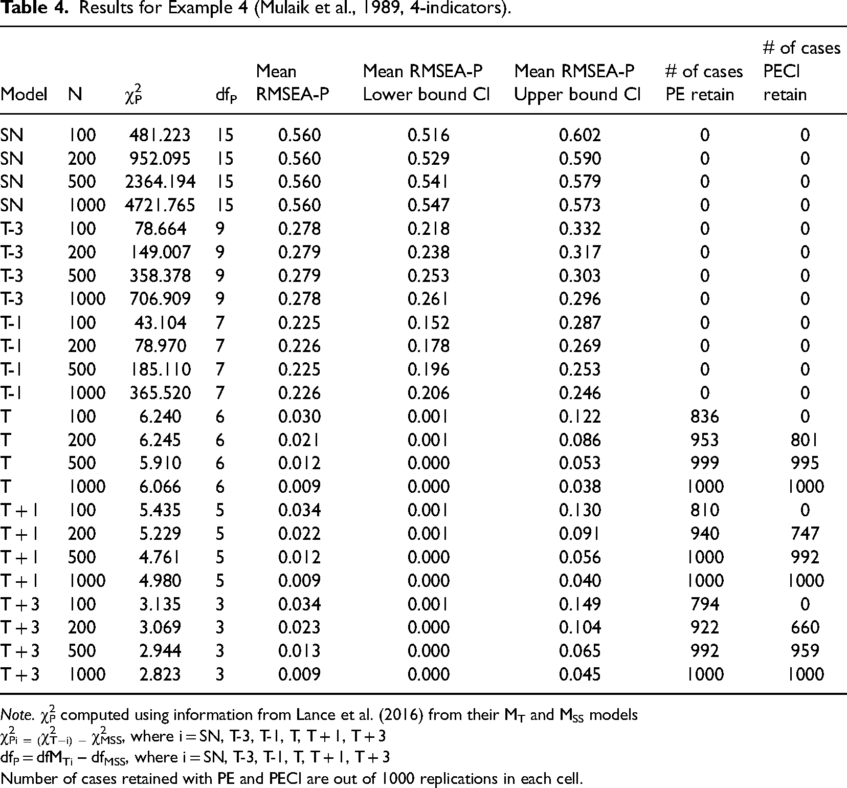
Note. χ²_P computed using information from Lance et al. (2016) from their M_T and M_SS models

χ²_{Pi = (}χ²_{T−i) −} χ²_MSS, where i = SN, T-3, T-1, T, T + 1, T + 3

df_P = dfM_Ti – df_MSS, where i = SN, T-3, T-1, T, T + 1, T + 3

Number of cases retained with PE and PECI are out of 1000 replications in each cell.

Examples 5 and 6. The next two examples are different from the first four in that they each contain a large number of latent variables represented by single indicators. Example 5 was based on a model originally published by Duncan et al. (1971) and is different in that most of its variables were only measured using a single indicator with no provision for measurement error. Specifically, this model includes six correlated exogenous variables, each measured using only a single indicator, and two endogenous latent variables involved in a non-recursive relationship, both measured using two indicators. Thus, three-fourths of the latent variables in this model were assessed with only a single indicator. As shown in Table 5, across the two smaller sample sizes for M_T−3 it would have been evaluated as supported (.070, .076) based on mean RMSEA-P values with the PE approach. However, using the PECI, M_T−3 would be rejected at all sample sizes as the upper bound to the CI was greater than .10 (.105 to .145). For M_T−1, the mean RMSEA-P values were also all less than .05 (ranging from .024 to .03), while the upper bound CI values were <.10 leading to model retention with the three larger sample sizes. Moving to the case level, use of the PE approach resulted in retention of many misspecified models based on RMSEA-P less than .08, ranging from 338 to 553 cases for M_T−3 and from 846 to 1000 cases with M_T−1. With the PECI approach, when taking into account confidence intervals, M_T−3 was retained less frequently in the three larger sample sizes (from 155 to 273 of the cases), while for M_T−1 the frequency of retention increased to 749–1000.

Table 5.
Results for Example 5 (Duncan et al., 1971, 2-indicators).

Model N χ²_P df_P Mean RMSEA-P Mean RMSEA-P Lower bound CI Mean RMSEA-P Upper bound CI # of cases PE retain # of cases PECI retain

SN 100 110.939 14 0.263 0.215 0.307 0 0

SN 200 210.618 14 0.265 0.232 0.296 0 0

SN 500 503.074 14 0.264 0.244 0.284 0 0

SN 1000 987.158 14 0.264 0.250 0.277 0 0

T-3 100 11.777 7 0.070 0.009 0.145 553 0

T-3 200 16.693 7 0.076 0.019 0.124 519 222

T-3 500 32.457 7 0.083 0.048 0.111 421 273

T-3 1000 58.994 7 0.085 0.064 0.105 338 155

T-1 100 5.098 5 0.030 0.001 0.127 846 0

T-1 200 5.268 5 0.023 0.001 0.091 938 749

T-1 500 6.676 5 0.022 0.001 0.063 993 968

T-1 1000 9.220 5 0.024 0.003 0.051 1000 1000

T 100 3.844 4 0.027 0.000 0.133 856 0

T 200 4.004 4 0.021 0.000 0.095 932 722

T 500 4.124 4 0.014 0.000 0.061 1000 985

T 1000 4.098 4 0.010 0.000 0.043 1000 1000

T + 1 100 3.128 3 0.034 0.000 0.148 803 0

T + 1 200 2.927 3 0.021 0.000 0.102 933 683

T + 1 500 3.134 3 0.015 0.000 0.066 990 945

T + 1 1000 3.002 3 0.010 0.000 0.046 999 999

T + 3 100 1.031 1 0.036 0.000 0.196 784 0

T + 3 200 1.054 1 0.026 0.000 0.138 859 0

T + 3 500 1.052 1 0.016 0.000 0.087 959 796

T + 3 100 0.914 1 0.010 0.000 0.060 996 960

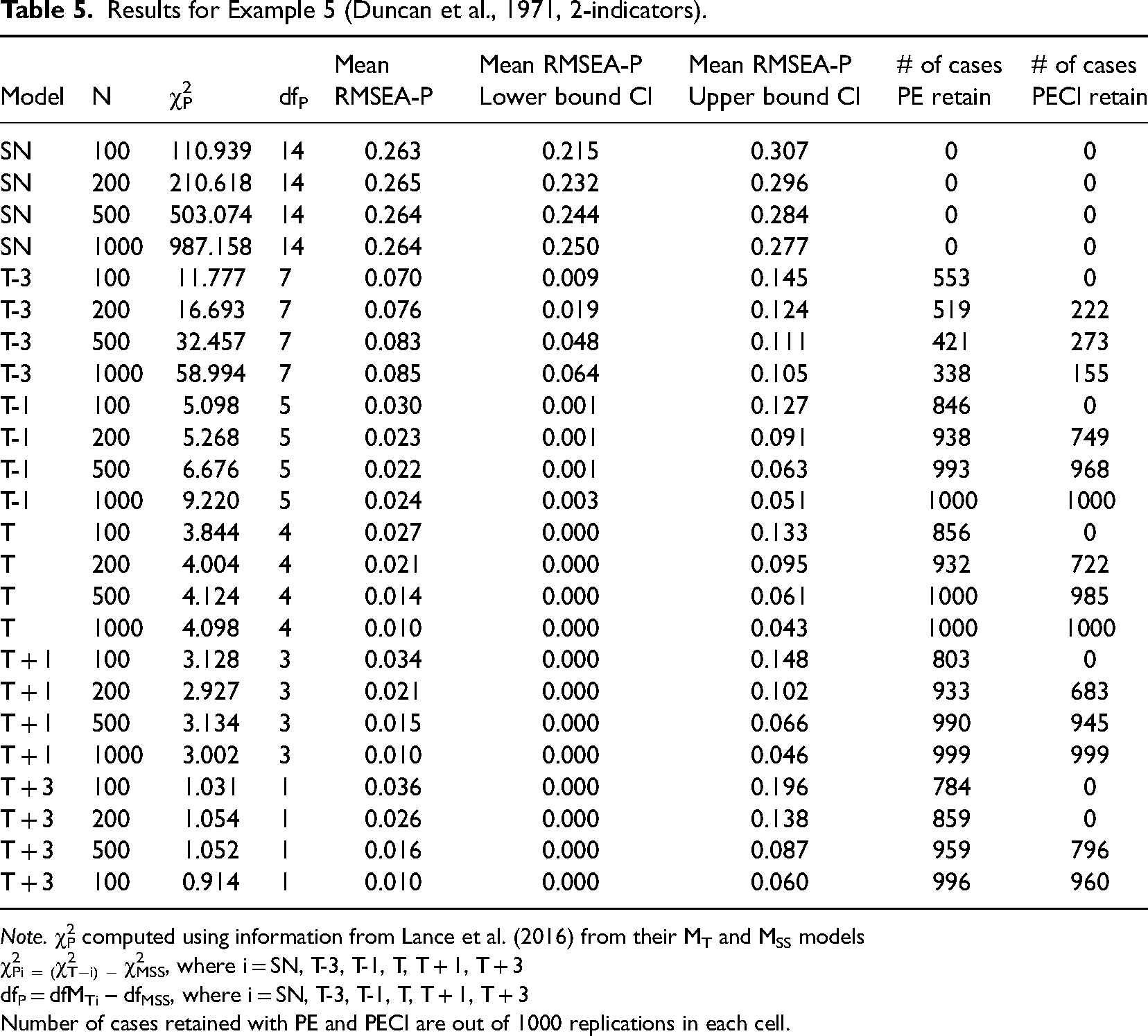
Note. χ²_P computed using information from Lance et al. (2016) from their M_T and M_SS models

χ²_{Pi = (}χ²_{T−i) −} χ²_MSS, where i = SN, T-3, T-1, T, T + 1, T + 3

df_P = dfM_Ti – df_MSS, where i = SN, T-3, T-1, T, T + 1, T + 3

Number of cases retained with PE and PECI are out of 1000 replications in each cell.

For M_T, all mean RMSEA-P point estimates and confidence intervals met criteria for their retention in the three larger sample sizes. The PE approach led to support for M_T from 856 to 1000 cases as sample size increased from 100 to 1000. Using the PECI, with the smallest sample size, correct identification of M_T never occurred, while for the three larger sample sizes, support was obtained from 722 to 1000 cases. In combination, these results for Example 5 show that for M_T−3 at the case level use of the RMSEA-P with the PECI approach resulted in mis-specified models being retained less (0%, 22.2%, 27.3%, 15.5% of cases) compared to M_T−1 (0%, 72.2%, 98.5%, 100% of cass). Incorrect retention occurred more often in the three larger sample sizes. For M_T, RMSEA-P PECI results correctly supported M_T in 0%, 72.2%, 98.5%, and 100% of the cases across the four sample sizes, with the greatest success occurring with the three larger sample sizes.

Finally, Example 6 incorporates a latent variable longitudinal panel design from Ecob (1987), in which two latent variables are assessed at three points in time, and the two are linked via lagged (but not within time period) relations. One of the latent variables is represented by a single indicator at each time point, while the other is measured using three indicators. Thus, half of the latent variables in this model were assessed with only a single indicator. Results in Table 6 revealed that like the first four examples, with use of mean RMSEA-P and CI values, all misspecified models were correctly identified as such. For M_T−3, mean RMSEA-P values were greater than .08 for all four sample sizes and all upper end values were greater than .10, indicating correct rejection. For M_T−1, while all mean RMSEA-P point estimates were less than .08 across the four sample sizes, all upper-bound mean CI estimates were greater than .10, also indicating correct rejection. When looking at individual samples with the PE approach, misspecified models were retained for M_T−3 in from 3 to 376 cases, and for M_T−1 from 521 to 608 cases as sample size decreased. With the PECI approach, such support occurred much less frequently for M_T−3, ranging from 0 to 43 of the 1000 cases, and from 0 to 325 for M_T−1.

Table 6.
Results for Example 6 (Ecob, 1987).

Model N χ²_P df_P Mean RMSEA-P Mean RMSEA-P Lower bound CI Mean RMSEA-P Upper bound CI # of cases PE retain # of cases PECI retain

SN 100 130.398 12 0.314 0.264 0.362 0 0

SN 200 249.670 12 0.315 0.280 0.348 0 0

SN 500 631.899 12 0.321 0.300 0.343 0 0

SN 1000 1270.249 12 0.324 0.309 0.339 0 0

T-3 100 10.733 5 0.094 0.014 0.175 376 0

T-3 200 17.903 5 0.108 0.038 0.160 223 43

T-3 500 42.234 5 0.120 0.083 0.153 23 8

T-3 1000 79.938 5 0.121 0.097 0.144 3 2

T-1 100 4.814 3 0.063 0.003 0.170 608 0

T-1 200 6.507 3 0.064 0.006 0.136 593 279

T-1 500 12.394 3 0.073 0.021 0.115 566 286

T-1 1000 22.603 3 0.079 0.042 0.108 521 325

T 100 1.976 2 0.032 0.000 0.163 811 0

T 200 1.950 2 0.022 0.000 0.115 889 649

T 500 2.077 2 0.015 0.000 0.073 982 890

T 1000 2.081 2 0.011 0.000 0.052 1000 997

T + 1 100 1.243 1 0.044 0.001 0.203 752 0

T + 1 200 1.004 1 0.024 0.000 0.137 874 0

T + 1 500 1.070 1 0.016 0.000 0.088 947 800

T + 1 1000 1.002 1 0.011 0.000 0.061 994 954

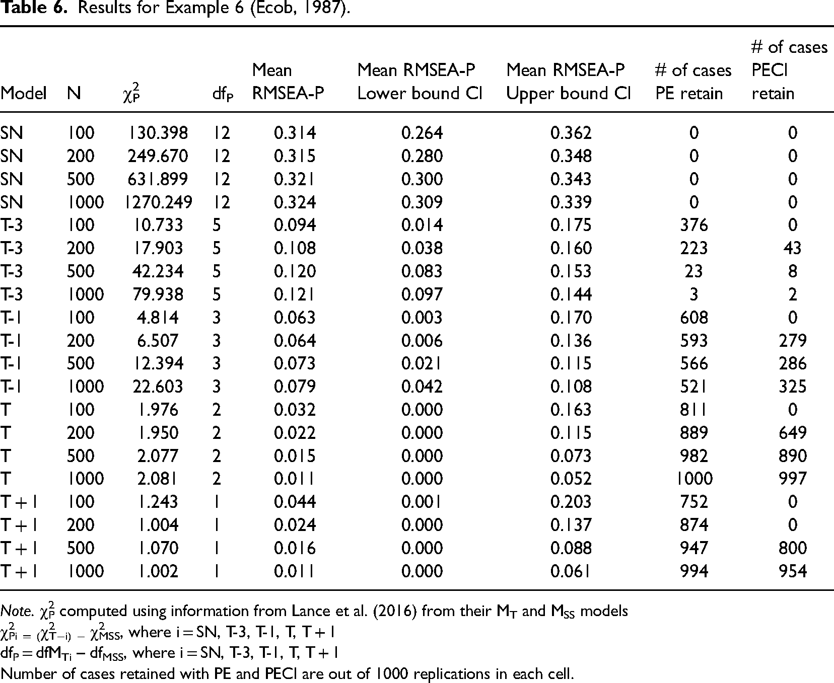
Note. χ²_P computed using information from Lance et al. (2016) from their M_T and M_SS models

χ²_{Pi = (}χ²_{T−i) −} χ²_MSS, where i = SN, T-3, T-1, T, T + 1

df_P = dfM_Ti – df_MSS, where i = SN, T-3, T-1, T, T + 1

Number of cases retained with PE and PECI are out of 1000 replications in each cell.

The results for M_T indicated mean RMSEA-P values less than .08 across all four sample sizes and low end values CI less than .05; however high end CV values less than .10 were obtained only with the two larger sample sizes (.052,.073). Use of the PE approach resulted in support for M_T ranging from 811 to 1000 cases across the four sample sizes, while the PECI approach did not support M_T in any cases when n = 100. For the three larger sample sizes, support was obtained from 649 to 997 cases. In combination, these results for Example 6 show that at the case level use of the RMSEA-P with the PECI approach resulted in misspecified models being retained in around 13% of the cases with M_T−3 and about 22% of the time with M_T−1, with incorrect retention occurring more often in larger sample sizes. Our RMSEA-P PECI results for this example correctly supported M_T in 64% of the cases across the four sample sizes, with the greatest success occurring with the three larger sample sizes.

We next report key findings based on the PE and PECI approaches in a way that allows comparison of our findings with those of Lance et al. (2016) and for consideration of differences among our six examples results. Table 7 presents descriptive RMSEA-P results and the percentage of cases for which each of three key models were retained, for combinations of the six examples used (Examples 1–4, Examples 5 and 6) and the four sample sizes examined. We have added row numbers to facilitate our presentation.

Table 7.
Comparison of RMSEA-P and % of Cases Combining Examples with Lance et al. (2016).

Model N

Row 100 200 500 1000

T-3 1 Lance Ex 1-6 PE 42 50 54 54

2 Ex 1-6 PE 15 12 7 6

3 Ex 1-6 PECI 0 4 5 3

4 Ex 1-4 PECI 0 0 0 0

5 Ex 5-6 PECI 0 13 14 8

6 Mean RMSEA-P and CI limits 0.287 (0.215–0.358) 0.292 (0.238–0.341) 0.296 (0.263–0.326) 0.296 (0.274–0.318)

T-1 7 Lance Ex1-6 PE 20 8 0 0

8 Ex 1-6 PE 24 25 26 25

9 Ex 1-6 PECI 0 17 21 22

10 Ex 1-4 PECI 0 0 0 0

11 Ex 5-6 PECI 0 51 63 66

12 Mean RMSEA-P and CI limits 0.227 (0.145–0.319) 0.228 (0.17–0.292) 0.23 (0.191–0.271) 0.232 (0.203–0.26)

T 13 Lance Ex1-6 PE 36 44 45 46

14 Ex 1-6 PE 81 91 98 100

15 Ex 1-6 PECI 0 49 91 98

16 Ex 1-4 PECI 0 40 90 98

17 Ex 5-6 PECI 0 68 94 100

18 Mean RMSEA-P and CI limits 0.033 (0.001–0.156) 0.023 (0–0.11) 0.014 (0–0.069) 0.01 (0–0.049)

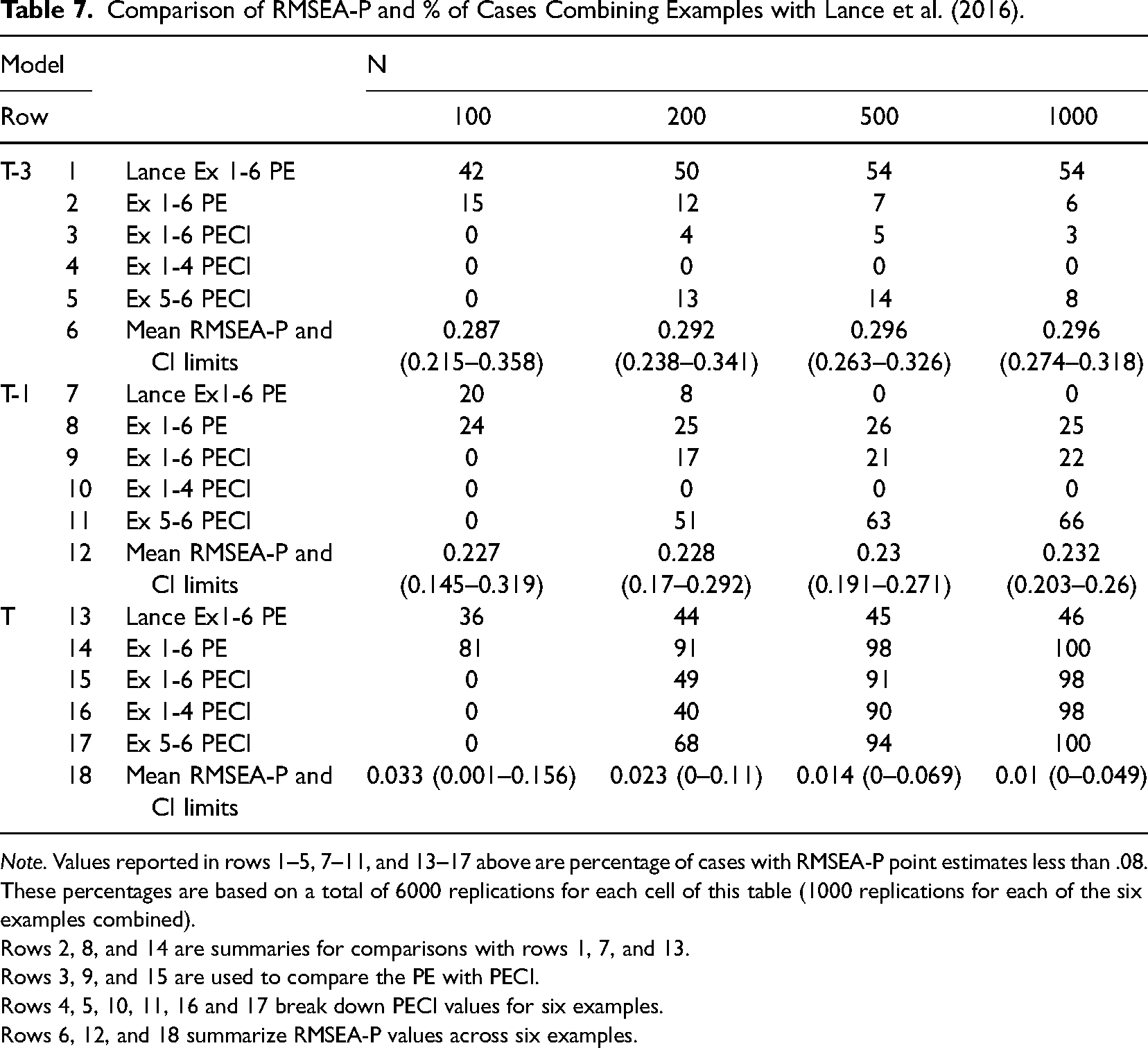
Note. Values reported in rows 1–5, 7–11, and 13–17 above are percentage of cases with RMSEA-P point estimates less than .08. These percentages are based on a total of 6000 replications for each cell of this table (1000 replications for each of the six examples combined).

Rows 2, 8, and 14 are summaries for comparisons with rows 1, 7, and 13.

Rows 3, 9, and 15 are used to compare the PE with PECI.

Rows 4, 5, 10, 11, 16 and 17 break down PECI values for six examples.

Rows 6, 12, and 18 summarize RMSEA-P values across six examples.

For each of the three models, the first row of information (rows 1, 7, 13) presents the percentage of cases retained based on use of the PE approach as reported by Lance et al. (2016), while the second row (rows 2, 8, 14) presents our PE results across all six examples (matching their presentation). A comparison of rows 1 and 2 shows that for M_T−3, this model was retained much more frequently by Lance et al. (e.g., 42% vs. 15% for n = 100), a pattern maintained across the other three sample sizes. Alternatively, M_T−1 was concluded to meet PE criteria less frequently by Lance et al. compared to our results across the four sample sizes (e.g., rows 7–8, 20% vs. 24% for n = 100). For M_T, PE results showed that Lance et al. reported support much less frequently compared to our findings (row 13, 36%–46%; row 14, 81%–100% of cases).

Regarding the PECI, the third row of information for each of the three models (rows 3, 9, 15) presents model retention rate across all six examples based on use of the PECI. A comparison of row 3 with row 2 shows that across all sample sizes use of the PECI with M_T−3 results in fewer incorrect models being retained in our results (0%–5% vs. 6%–15%). A similar pattern is found for M_T−1 with the comparison of rows 8 vs. 9. This occurs because models with RMSEA-P estimates less than .08 but upper bound confidence intervals greater than .10 are retained with the PE approach but not the PECI approach, especially with small samples.

The next two rows of information for each of the three models present PECI findings for two groups, Examples 1-4 in which all latent variables are represented with multiple indicators, and Examples 5 and 6 in which single indicators are used for over half of the latent variables. A comparison of these two rows (rows 4 and 10) for Models M_T−3 and M_T−1 shows that in Examples 1–4, there were no cases in which a misspecified model was incorrectly supported; all cases of these two models being incorrectly retained occurred only with Examples 5 and 6 (rows 5 and 11).

The results in Table 7 also show mean RMSEA-P and CI values from our simulated data (rows 6, 12, 18) for three key models (M_T−3, M_T−1, M_T), combined across all six examples but reported separately for the four sample sizes. We report these mean values to allow further exploration of the differences between our results and the findings of Lance et al. (2016) reported in their Table 11. We focus on two cases (M_T−3, M_T, both with N = 1000). As shown in row 6 of Table 7, for the case in which the misspecified model M_T−3 is considered with a sample size of 1000, our mean value for the RMSEA-P is .296 (with mean confidence interval bounds of .274 and .318). These RMSEA-P mean values are consistent with our individual sample results-as already presented in Tables 5 and 6; we found for M_T−3 with N = 1000 that in only 5.6% of the 6000 cases of the six examples (338 + 3 = 341) was the RMSEA-P less than .08. By comparison, Lance reported for M_T−3 that 54% of their cases had values less than .08 with N = 1000 (row 1). Next, as shown in row 18 for the true model M_T we obtained a mean RMSEA-P value of .010 with N = 1000 (with confidence interval bounds of .0 and .049). We add that our individual case values also match what would be expected given these RMSEA-P values—we found all cases to have RMSEA-P values less than .08 (the correct model was identified in all cases—row 14). In contrast, Lance et al. reported obtaining RMSEA-P values less than .08 in only 46% of their samples (row 13). In sum, these results show that findings from Lance et al. are very inconsistent with both our mean RMSEA-P values and our individual case results.

Supplemental Analysis of Data

Having demonstrated the match of our data (chi-square, df, RMSEA-P) with that of Lance et al., we further explored the extreme differences between our findings and those of Lance et al. (2016). We conducted additional analyses using some of their data reported in their Tables 2–8 (p. 394−399). As described in our Appendix, these analyses focused on one case from each of our six examples, the case of M_T−3 with a sample size of 1000. We chose these six examples because they are cases where our results were most different from Lance et al.'s findings. The chi-squares and degrees of freedom for these six cases from Lance et al.'s data are presented in our Appendix Table, Part A, columns 1–3. We computed values of RMSEA-P and related confidence intervals with their data and these are shown in our Appendix Table, Part B, columns 4–6. We first note that these values are nearly identical to corresponding values from our simulated data as presented in Tables 1–6, indicating the match between our data generation approach and Lance et al.'s simulation approach. Thus, we can eliminate as an explanation of the differences between our results and those of Lance et al., any concern about the underlying data being different.

Next, we demonstrate that these computed RMSEA-P mean and confidence intervals using Lance et al.'s data are inconsistent with their reported results for RMSEA-P point estimates shown in their Table 11. Specifically, for M_T−3 they reported a high percentage of cases (54%) with RMSEA-P values less than .08 across the six examples with a total of 6000 replications. Such a high number of cases with RMSEA-P less than .08 seems very unlikely given the mean RMSEA-P and confidence values from their data for these six examples presented above in Appendix B, Part B, rows 4–6. To illustrate, we combined the RMSEA-P values and confidence intervals from the six examples (Appendix columns 4–6) and obtained an overall value of .296 and confidence interval end points of .274 and .318. Given an interpretation of the confidence intervals that 90% of the RMSEA-P values would be expected to fall between .274 and .318, it seems very unlikely Lance et al. would find 54% of the values from this same data to have values less than .08.

The results above based on our analyses of data taken directly from Lance et al.'s data raise questions about the accuracy of the 54% value for the number of cases with an RMSEA-P <.08. Thus, as described in our Appendix, we further explored results from Lance et al. through a Theoretical Analysis based on their data. Our analysis followed the approach used to investigate RMSEA performance with true models by Kenny, Kaniskan, and McCoach (2015). Our objective was to determine theoretically the expected number of cases with RMSEA-P values <.08 for the 6000 cases across the six examples. As presented in our Appendix, these theoretical results show that for M_T−3 and a sample size of 1000 across the six examples, only 5.5% of cases would be expected to have RMSEA-P values less than .08. This value matches very closely results already presented in this paper from our simulations in which we found 5.6% of our 6000 sample replication values had RMSEA-P values less than .08. In sum, both our simulation results and the results of our theoretical analysis, 5.5% and 5.6% with RMSEA-P values less than .08 are very different from the 54% value reported in Table 11 of Lance et al. (2016).

Discussion

The present research investigates the RMSEA-P combining the strengths of two previous simulation studies, including examination of results at the case level for each of six examples separately based on four sample sizes while using point estimates and confidence intervals. Although Williams and O’Boyle (2011) did not examine results at the case level, the present findings are consistent with what they reported. They found the RMSEA-P to effectively distinguish between true and mis-specified models for five of the examples, while with the sixth example (Duncan, et al., 1971, our Example 5) M_T was correctly identified but misspecified models with one or two true paths omitted also were retained. It should be noted that Williams and O’Boyle (2011) were using previously published data and only reported results for N = 500, and the number of replications in each cell of their design was only 20. Thus, our current findings are more reliable since we used 1000 replications, and more generalizable since we examined results based on four sample sizes. In contrast, our results are very different from those shown in Table 11 of Lance et al. (2016). And, these differences occurred even though our data generation began with their information (we used their chi-square values as population values) and we used a standard approach to generating our sample chi-square values using R. Moreover, as shown in our Appendix, our reanalysis using Lance et al.'s published results for six specific cases yielded conclusions inconsistent with their reported finding of a high percentage of individual cases of RMSEA-P values less than .08 with a severely misspecified model (M_T−3). Finally, we also demonstrated that the results of these six cases are very inconsistent with those predicted by statistical theory. Having demonstrated the validity of our data and conclusions, while also showing serious problems with findings of Lance et al., we now focus on the implications of our results.

The results presented in Tables 1–7 allow several important conclusions. First, regarding differences across examples, the RMSEA-P was very effective with Examples 1–4 at identifying misspecified and correct models. For incorrectly specified models M_T−3 and M_T−1, combining across four examples (Tables 1–4) with 4000 sample results, there were only two sample RMSEA-P point estimate values that did not exceed the recommended cut-off of. 08 (see Table 3 results for M_T−1 from Example 3). When confidence intervals are incorporated, as with PECI, results from Table 7 show that for these four examples combined there were no cases where the PECI approach resulted in retention of an incorrectly specified model (row 4 for M_T−3 and row 10 for M_T−1). This finding is in strong contrast to results from Lance et al., who found the RMSEAP retained severely misspecified models—for example, see row 1 of Table 7. The fact that the RMSEA-P correctly identified misspecfied models is important because if, instead, these models were retained the interpretation of the paths from the model would be compromised. This would occur because the influence of the omitted paths will be captured in the estimates of paths that are in the model, leading them to be biased.

For true models M_T, with these first four examples, our results from Tables 1–4 show the RMSEA-P performed well, especially with sample sizes greater than 200. As shown in these tables, across the four sample sizes examined, PE estimates for M_T were very frequently less than .08, indicating acceptable fit (ranging from 77% to 100%). For the two larger sample sizes (n = 500, 1000), this occurred in over 97% of the 4000 cases in Examples 1–4. For the two smaller sample sizes (n = 100, 200), this occurred in between 77% and 95% of the cases with an average success rate of 86%. This pattern is in direct contrast to Lance et al., who across all sample sizes found M_T to be correctly retained in less than 50% of the cases using the .08 RMSEA-P cut-off (see row 13, Table 7). Inclusion of the confidence interval information with use of PECI also showed success with sample sizes over 200, in that M_T was successfully identified in 90% and 98% of cases (Table 7, row 16). However, when the sample size was 200, this success rate dropped to 40% and with a sample size of 100, no cases had supportive RMSEA-P conclusions using confidence intervals. We will further discuss the implications of sample size effects on confidence intervals with the RMSEA-P in our recommendations section. This overall pattern of findings above is consistent with previous results of Williams and O’Boyle (2011) but is very different from results presented by Lance et al. (2016), who did not distinguish between six example models and reported combined results while not using confidence intervals.

Regarding differences across examples, our findings in Table 7 for Examples 5 and 6 show the RMSEA-P was less effective and illustrate key differences in results for the six example models. In contrast to Examples 1–4, with Examples 5 and 6 M_T−3 was supported with the PECI approach in 8%–14% of the cases with the three larger sample sizes (row 5), while for M_T−1 support increased to 51%–66% of the cases (row 11). Thus, in these two examples, use of the RMSEA-P and the PECI approach would more often than desired lead to incorrect model retention. The key conclusion is that across sample sizes with Examples 1–4 when multiple indicators are used for all latent variables, if the RMSEA-P is used with the PECI approach, researchers can count on the RMSEA-P to properly reject an incorrect latent variable model. And with moderate sample sizes (>200), researchers can be confident that they can correctly identify a true model if the PECI approach is applied. For our Example 5 and 6 models with fewer indicators, use of the PECI may lead to retention of some mis-specified models and rejection of some correctly specified models. We now note that while our discussion of Examples 5 and 6 has focused on their fewer indicators, there is a different design feature that may explain why their results are different from those of the other four examples.

This explanation focuses on the magnitudes of the paths dropped to create the misspecified models. As described by Lance et al. (2016), in their study, misspecified models were developed by first removing paths with the lowest population values. For these two examples, the paths that were dropped in creating the misspecified models M_T−3 and M_T−1 had relatively smaller parameter values compared to those of Examples 1–4 (see path values shown in Figures 1–6 from Lance et al., 2016). With Example 5 based on Duncan et al. (1971), the paths dropped had values of .08, .09, and .19, while for Example 6 based on Ecob (1987), the three paths dropped had values of −.14, −.14, and −.16. These values are much lower than the values of the first three paths dropped in the other examples (each .4). These lower path values, rather than the number of indicators, may have led to models being retained that excluded these paths with use of the RMSEA-P. To pursue this explanation, Williams and Castille (2021) increased the magnitude of these three paths in an analytical simulation and found that as these paths were increased in magnitude, RMSEA-P became more effective at identifying M_T−3 as a misspecified model. Additional support for this alternative explanation is based on the similarity of RMSEA-P effectiveness in Examples 1 vs. 2 and Examples 3 vs. 4, which differed only in the number of indicators used to measure the latent variables. Finally, we add that with many sample sizes, paths of such small magnitude in a model would not likely be statistically significant. As a result, RMSEA-P support for models with these paths left out (e.g., M_T−3) can be seen more favorably since these models would not have misspecifications (because the paths left out are not significant). And, we note the estimates for the paths in the model would not be expected to biased by the omission of the non-significant paths and related conclusions about these paths would remain valid.

A second general finding from our results is that use of confidence intervals with the PECI approach makes a difference in conclusions about rejecting vs. failing to reject a model, as compared to the PE approach. For misspecified models, the use of confidence intervals showed that across all six examples, many models retained based on only point-estimates would be rejected when use of confidence intervals is incorporated as we did in the model evaluation process. For example, as shown in Table 7 use of the PE approach when sample size was 100 with M_T−3 resulted in model retention for 15% of cases (row 2), and this success dropped to 0% with PECI (row 3); for M_T−1 when sample size was 200 model retention dropped from 25% to 17% with PE vs. PECI. As suggested earlier, this shows that in many cases, incorrect models with PE estimates less than .08 but higher bounds of confidence intervals greater than .10 will be correctly rejected if confidence intervals are examined. Thus, in these cases, the RMSEA-P using confidence intervals works well at lowering the frequency of incorrect retention of misspecified models. Our results in Table 7 show this was true of the findings of Lance et al. (2016), who retained many more incorrect models across all sample sizes using only point-estimates than we did using the PECI. These findings reflect favorably on the RMSEA-P—they indicate that a model with misspecifications will be much more likely to be correctly rejected if confidence intervals are used with the PECI approach.

Compared to misspecified models, for true models, our results showed that use of confidence intervals with the PECI resulted in some M_T models being rejected in smaller sample sizes that would have been retained if only the point estimates were examined. Across all six examples, favorable RMSEA-P point estimates less than .08 occurred in 81% and 91% of cases with the two smaller sample sizes (row 14), but with use of confidence intervals in the PECI approach model results supporting M_T occurred much less frequently (in 0% and 49% of cases, respectively, row 15). Thus, inclusion of the confidence interval with the RMSEA-P can help researchers realize the limits of their conclusions when they obtain supportive point-estimates with small sample sizes. Use of confidence intervals may also help them correctly identify misspecified models that they might otherwise accept if only point-estimates were examined. In spite of these advantages, use of confidence intervals with fit measures seems to be rare in organizational and management research. For example, Williams, O’Boyle, and Yu (2020) reported that less than 10% of 316 studies in their review used RMSEA confidence intervals. Hopefully our comparison of the success of the PECI relative to the PE approach may increase their use by organizational researchers. However, researchers wanting to include confidence intervals for the RMSEA-P with the evaluation of their models should carefully consider how they are used, and two perspectives seem possible.

The results and conclusions we report are based on one approach, a traditional use in which a model is completely rejected if the upper end of the confidence interval is greater than .10. This approach has been described by Kline (2015) as a test of the poor-fit hypothesis, a “reject-support test of whether the researchers model is just as bad as or even worse than a poor fitting population model” (p. 275). Followers of this approach may have concerns about our findings that the use of RMSEA-P and confidence intervals can lead to rejection of true models with smaller sample sizes. Alternatively, a second approach with the RMSEA suggests that a model not be automatically rejected because the upper end of a confidence interval is greater than .10. This view is reflected in the perspective by Brown and Cudeck (1993) that these intervals remind researchers of the limits of their sample point estimates. As noted by Browne and Cudeck (1993), confidence intervals “supplement point-estimates by interval estimates to bring the lack of precision of the estimates to the users attention” (p. 138). Subsequently, MacCallum, Browne, and Sugawara (1996) stated that confidence intervals “provides information about precision of the estimate and can greatly assist the researcher in drawing appropriate conclusions about model quality” (p. 134). More recently, as noted by Kline (2015, p. 139) the use of the confidence interval with the RMSEA “reflects the degree of uncertainty associated with the RMSEA as a point-estimate”, and “acknowledges that the RMSEA (and all other model fit indices) are sample statistics subject to sampling error” (Kline, 2015, p. 139). These views seem to suggest a broader use of confidence intervals, in contrast to their use in a binary null-hypothesis test regarding poor fit. If one prefers this less restrictive view and favors use of confidence intervals as a reminder of the limitations of one's data, our results with the RMSEA-P can be seen more favorably.

Our findings show that when one's true model has paths of reasonable magnitude and multiple indicators are used, RMSEA-P point estimates are less than .08 in a very high percentage of cases. The finding that with small sample sizes, the upper end of the confidence interval of these estimates may frequently exceed .10 may suggest that rather than leading to the rejection of the model in a binary way, it should lead the researcher to encourage further investigation of the model with larger sample sizes. Indeed, MacCallum et al. (1996) also stated that in such cases of a low RMSEA value but a wide confidence interval “the investigator could recognize that there may be substantial imprecision in their RMSEA estimate, in which case one cannot determine accurately the degree of fit in the population” (our italics, p. 134). In other words, in these circumstances, it may be premature to reach any final decision about the ultimate quality of the model until further evidence is examined. More recently, in a similar circumstance, Klein (2015) noted that when facing estimate imprecision and accompanying ambiguity when hypothesis testing, researchers should obtain a larger sample rather than rejecting the model (p. 275).

Our third conclusion based on our results concerns how path model fit indices should be used in the broader process of model evaluation. We begin by reviewing that for model confirmation a key condition needs to be met, referred to by James, Mulaik, and Brett (1982) as Condition 10, that focuses on evidence that paths left out of any theoretical model (M_T) are correctly omitted. Three types of information can be used, and we present the three approaches and provide some comments on their use as background for a subsequent recommendation for their combined use. First, the results of a formal model comparison can be examined based on a chi-square difference test of M_T with a model that adds paths linking all latent variables with each other (referred to as a saturated structural model, M_SS, that is equivalent in fit to a correlated factors model). This approach was given priority by James et al. and Anderson and Gerbing (1988). The researcher hopes this chi-square difference test is not statistically significant, leading to the conclusion that the added paths should not be included. A concern with this Condition 10 approach is that the high statistical power of the test can lead to rejection even when differences in the amount of explained covariances among the indicators due to the added paths is minimal. In other words, this test can be seen to suffer the limitations of the overall chi-square test as a measure of perfect fit, where the fit is focused on paths added and the test is whether their associated residual covariances as a set are zero.

A second type of Condition 10 test involves the statistical significance of the paths originally predicted to be zero that are added to M_T to create M_SS. The researcher hopes the added paths are not individually statistically significant, supporting their omission in M_T. A concern with this approach can be the absence of theory to support the direction of the added paths. If there is no theory for the added paths, which is likely or the paths would have been in the original model M_T, the choice of direction of any path is arbitrary. Moreover, for such a saturated structural model there could be many specifications different from the one chosen by the researcher that would yield “equivalent” model fit. Williams et al. (1996) and Williams (2012) have shown that path estimates and their statistical significance can vary dramatically across equivalent fitting models. Thus, any conclusions about the importance of these statistically significant added paths is of limited value—had the researcher chosen a different specification with paths in a different direction, different patterns of significance would likely be obtained.

The third type of Condition 10 evidence involves goodness of fit measures, of which the RMSEA-P is a special case that focuses on the path component. James et al. (1982) and Anderson and Gerbing (1988) noted that goodness of fit measures should play a supplemental role to these two first two Condition 10 tests. In the seminal article on such measures, Bentler and Bonett (1980) stated that fit indices can “provide information about practical significance, in which a statistically significant effect can be evaluated for its practical usefulness in explaining the data” (p. 599). Or as stated by Kelley and Preacher (2012), the RMSEA (and by extension RMSEA-P) can be seen as “an operationalization of the estimated effect size dimension of model fit” in the context of structural equation models (p. 141). Given this tradition, perhaps the restrictive use of the RMSEA-P confidence interval as a reject/support binary tool for model evaluation is not the best approach. The RMSEA-P, as with the original RMSEA, can be seen as providing a summary of path model misfit per degree of freedom that also includes a confidence interval allowing judgment about performance of the model beyond the sample whose results are being considered. And, the RMSEA-P overcomes the important limitation that the traditional global fit index RMSEA has been demonstrated to support models with extreme misspecifications in the six examples of this study (Williams & O’Boyle, 2011) and in published management research (Williams, O’Boyle, & Yu, 2020).

Recommendations

Given these considerations, we believe that all three approaches to Condition 10 evaluation described above can play an important role, as their individual effectiveness may vary across situations (for example, sample size, path magnitude). Overall, our findings suggest a key recommendation for a researcher, especially when working with a relatively low sample size—make sure to consider the results of all three Condition 10 tests. If the RMSEA-P index is used to evaluate M_T with a low sample size and the obtained point estimate is less than .08 but the upper bound of its confidence interval is greater than .10, additional information should be considered before rejecting M_T. If the chi-square difference test of M_T with M_SS is not significant and/or the paths added to form M_SS are not themselves statistically significant, this may suggest the non-supportive upper limit of the confidence interval may reflect lower power of the RMSEA-P and M_T should be tentatively retained for future evaluation. The use of these statistical tests as supplements to the RMSEA-P help researchers avoid what could be incorrect rejection of M_T and allow them to be more confident that their model does not contain important misspecifications. The likely different statistical power of these three statistical tests for Condition 10 suggests using all three would be a good strategy. We note that the focus on individual paths is consistent with recommendations from Kenny, Kaniskan, and McCoach (2015) who encouraged looking at path parameter estimate significance. However, unlike Kenny et al., we feel the RMSEA-P still should continue to be examined, with balance given to interpretation of point estimates and confidence intervals (e.g., Browne & Cudeck, 1993; Klein, 2015; MacCallum et al., 1996). It should be remembered that in the case of inconsistent results across the three Condition 10 tests, a more cautious approach is warranted about the generalizability of the findings to the population, and more research is needed understanding different power of these tests and their sensitivity to model specification (e.g., McNeish, 2020).

Conclusions

We emphasize our belief that the best approach to model testing begins with evaluation and improvement of the measurement model linking latent variables to their indicators, as emphasized by Anderson and Gerbing (1988). However, even with an optimal measurement model, a researcher should not rely only on global fit indices as a Condition 10 test, as done by most organizational researchers (Williams, O’Boyle, Yu, 2020). Instead, confirming Condition 10 for any associated latent variable path models should involve the use of the PECI approach with the RMSEA-P, in combination with the significance of the M_T-M_SS chi-square difference test and the significance of the paths predicted to be zero. James, Mulaik, and Brett (1982) also describe a Condition 9 for model confirmation, and we believe the chi-square difference between M_T and the structural null, as well as the significance of paths included in M_T, should be used along with the NSCI-P recommended by Williams and O’Boyle (2011) and Lance et al. (2016). While traditional SEM software does not provide estimates of path model fit, a new package for path model assessment using lavaan with R is now available (pathmodelfit, https://cran.r-project.org/web/packages/pathmodelfit/index.html) which provides RMSEA-P and NSCI values, and an excel file for computing RMSEA-P and confidence intervals using chi-square and degrees of freedom values from theoretical and saturated structural (measurement) models is also available. Finally, we believe that both Condition 9 and Condition 10 tests should be examined before researchers conclude their model is viable, and they should also remember that even if these conditions are fulfilled, the possibility always remains that there may be one or more unexamined alternative models that may fit the data equally or better.

Model	N	χ²_P	df_P	Mean RMSEA-P	Mean RMSEA-P Lower bound CI	Mean RMSEA-P Upper bound CI	# of cases PE retain	# of cases PECI retain
SN	100	297.178	7	0.646	0.582	0.708	0	0
SN	200	585.300	7	0.644	0.599	0.687	0	0
SN	500	1457.740	7	0.644	0.616	0.672	0	0
SN	1000	2912.920	7	0.645	0.625	0.664	0	0
T-3	100	92.534	4	0.470	0.383	0.551	0	0
T-3	200	183.040	4	0.473	0.413	0.530	0	0
T-3	500	452.239	4	0.473	0.436	0.510	0	0
T-3	1000	894.610	4	0.472	0.446	0.498	0	0
T-1	100	37.783	2	0.419	0.291	0.532	0	0
T-1	200	73.078	2	0.419	0.333	0.499	0	0
T-1	500	182.141	2	0.424	0.370	0.475	0	0
T-1	1000	358.836	2	0.422	0.385	0.458	0	0
T	100	1.141	1	0.040	0.001	0.199	775	0
T	200	1.078	1	0.026	0.000	0.139	862	0
T	500	1.005	1	0.015	0.000	0.087	955	805
T	1000	1.024	1	0.011	0.000	0.061	992	950

Model	N	χ²_P	df_P	Mean RMSEA-P	Mean RMSEA-P Lower bound CI	Mean RMSEA-P Upper bound CI	# of cases PE retain	# of cases PECI retain
SN	100	295.916	7	0.645	0.58	0.706	0	0
SN	200	588.079	7	0.645	0.601	0.689	0	0
SN	500	1458.702	7	0.644	0.616	0.672	0	0
SN	1000	2912.538	7	0.644	0.625	0.664	0	0
T-3	100	85.729	4	0.451	0.364	0.532	0	0
T-3	200	171.560	4	0.457	0.397	0.515	0	0
T-3	500	427.296	4	0.46	0.423	0.496	0	0
T-3	1000	848.161	4	0.459	0.433	0.485	0	0
T-1	100	35.965	2	0.407	0.279	0.52	0	0
T-1	200	72.034	2	0.416	0.33	0.497	0	0
T-1	500	176.576	2	0.417	0.364	0.468	0	0
T-1	1000	350.419	2	0.417	0.379	0.453	0	0
T	100	1.017	1	0.036	0	0.195	784	0
T	200	0.991	1	0.024	0	0.137	870	0
T	500	1.087	1	0.017	0	0.088	943	780
T	1000	0.998	1	0.011	0	0.061	992	950

Model	N	χ²_P	df_P	Mean RMSEA-P	Mean RMSEA-P Lower bound CI	Mean RMSEA-P Upper bound CI	# of cases PE retain	# of cases PECI retain
SN	100	443.985	15	0.537	0.493	0.579	0	0
SN	200	870.240	15	0.535	0.504	0.565	0	0
SN	500	2171.066	15	0.536	0.517	0.555	0	0
SN	1000	4327.023	15	0.536	0.523	0.5	0	0
T-3	100	124.062	9	0.358	0.299	0.412	0	0
T-3	200	242.230	9	0.360	0.320	0.399	0	0
T-3	500	595.679	9	0.361	0.336	0.385	0	0
T-3	1000	1189.235	9	0.362	0.345	0.379	0	0
T-1	100	41.185	7	0.218	0.145	0.280	2	0
T-1	200	74.658	7	0.219	0.171	0.262	0	0
T-1	500	179.369	7	0.221	0.193	0.249	0	0
T-1	1000	352.468	7	0.222	0.202	0.241	0	0
T	100	6.690	6	0.035	0.001	0.125	822	0
T	200	6.192	6	0.021	0.001	0.086	960	797
T	500	6.084	6	0.013	0.000	0.054	1000	999
T	1000	5.893	6	0.009	0.000	0.038	1000	1000
T + 1	100	5.622	5	0.036	0.001	0.132	786	0
T + 1	200	5.323	5	0.023	0.001	0.091	940	743
T + 1	500	5.075	5	0.013	0.000	0.057	1000	994
T + 1	1000	5.011	5	0.009	0.000	0.040	1000	1000
T + 3	100	3.260	3	0.036	0.001	0.150	782	0
T + 3	200	3.185	3	0.025	0.001	0.105	902	656
T + 3	500	3.068	3	0.014	0.000	0.066	998	954
T + 3	1000	3.228	3	0.011	0.000	0.047	1000	999

Model	N	χ²_P	df_P	Mean RMSEA-P	Mean RMSEA-P Lower bound CI	Mean RMSEA-P Upper bound CI	# of cases PE retain	# of cases PECI retain
SN	100	481.223	15	0.560	0.516	0.602	0	0
SN	200	952.095	15	0.560	0.529	0.590	0	0
SN	500	2364.194	15	0.560	0.541	0.579	0	0
SN	1000	4721.765	15	0.560	0.547	0.573	0	0
T-3	100	78.664	9	0.278	0.218	0.332	0	0
T-3	200	149.007	9	0.279	0.238	0.317	0	0
T-3	500	358.378	9	0.279	0.253	0.303	0	0
T-3	1000	706.909	9	0.278	0.261	0.296	0	0
T-1	100	43.104	7	0.225	0.152	0.287	0	0
T-1	200	78.970	7	0.226	0.178	0.269	0	0
T-1	500	185.110	7	0.225	0.196	0.253	0	0
T-1	1000	365.520	7	0.226	0.206	0.246	0	0
T	100	6.240	6	0.030	0.001	0.122	836	0
T	200	6.245	6	0.021	0.001	0.086	953	801
T	500	5.910	6	0.012	0.000	0.053	999	995
T	1000	6.066	6	0.009	0.000	0.038	1000	1000
T + 1	100	5.435	5	0.034	0.001	0.130	810	0
T + 1	200	5.229	5	0.022	0.001	0.091	940	747
T + 1	500	4.761	5	0.012	0.000	0.056	1000	992
T + 1	1000	4.980	5	0.009	0.000	0.040	1000	1000
T + 3	100	3.135	3	0.034	0.001	0.149	794	0
T + 3	200	3.069	3	0.023	0.000	0.104	922	660
T + 3	500	2.944	3	0.013	0.000	0.065	992	959
T + 3	1000	2.823	3	0.009	0.000	0.045	1000	1000

Model	N	χ²_P	df_P	Mean RMSEA-P	Mean RMSEA-P Lower bound CI	Mean RMSEA-P Upper bound CI	# of cases PE retain	# of cases PECI retain
SN	100	110.939	14	0.263	0.215	0.307	0	0
SN	200	210.618	14	0.265	0.232	0.296	0	0
SN	500	503.074	14	0.264	0.244	0.284	0	0
SN	1000	987.158	14	0.264	0.250	0.277	0	0
T-3	100	11.777	7	0.070	0.009	0.145	553	0
T-3	200	16.693	7	0.076	0.019	0.124	519	222
T-3	500	32.457	7	0.083	0.048	0.111	421	273
T-3	1000	58.994	7	0.085	0.064	0.105	338	155
T-1	100	5.098	5	0.030	0.001	0.127	846	0
T-1	200	5.268	5	0.023	0.001	0.091	938	749
T-1	500	6.676	5	0.022	0.001	0.063	993	968
T-1	1000	9.220	5	0.024	0.003	0.051	1000	1000
T	100	3.844	4	0.027	0.000	0.133	856	0
T	200	4.004	4	0.021	0.000	0.095	932	722
T	500	4.124	4	0.014	0.000	0.061	1000	985
T	1000	4.098	4	0.010	0.000	0.043	1000	1000
T + 1	100	3.128	3	0.034	0.000	0.148	803	0
T + 1	200	2.927	3	0.021	0.000	0.102	933	683
T + 1	500	3.134	3	0.015	0.000	0.066	990	945
T + 1	1000	3.002	3	0.010	0.000	0.046	999	999
T + 3	100	1.031	1	0.036	0.000	0.196	784	0
T + 3	200	1.054	1	0.026	0.000	0.138	859	0
T + 3	500	1.052	1	0.016	0.000	0.087	959	796
T + 3	100	0.914	1	0.010	0.000	0.060	996	960

Model	N	χ²_P	df_P	Mean RMSEA-P	Mean RMSEA-P Lower bound CI	Mean RMSEA-P Upper bound CI	# of cases PE retain	# of cases PECI retain
SN	100	130.398	12	0.314	0.264	0.362	0	0
SN	200	249.670	12	0.315	0.280	0.348	0	0
SN	500	631.899	12	0.321	0.300	0.343	0	0
SN	1000	1270.249	12	0.324	0.309	0.339	0	0
T-3	100	10.733	5	0.094	0.014	0.175	376	0
T-3	200	17.903	5	0.108	0.038	0.160	223	43
T-3	500	42.234	5	0.120	0.083	0.153	23	8
T-3	1000	79.938	5	0.121	0.097	0.144	3	2
T-1	100	4.814	3	0.063	0.003	0.170	608	0
T-1	200	6.507	3	0.064	0.006	0.136	593	279
T-1	500	12.394	3	0.073	0.021	0.115	566	286
T-1	1000	22.603	3	0.079	0.042	0.108	521	325
T	100	1.976	2	0.032	0.000	0.163	811	0
T	200	1.950	2	0.022	0.000	0.115	889	649
T	500	2.077	2	0.015	0.000	0.073	982	890
T	1000	2.081	2	0.011	0.000	0.052	1000	997
T + 1	100	1.243	1	0.044	0.001	0.203	752	0
T + 1	200	1.004	1	0.024	0.000	0.137	874	0
T + 1	500	1.070	1	0.016	0.000	0.088	947	800
T + 1	1000	1.002	1	0.011	0.000	0.061	994	954

Model		N
T-3	1	Lance Ex 1-6 PE	42	50	54	54
	2	Ex 1-6 PE	15	12	7	6
	3	Ex 1-6 PECI	0	4	5	3
	4	Ex 1-4 PECI	0	0	0	0
	5	Ex 5-6 PECI	0	13	14	8
	6	Mean RMSEA-P and CI limits	0.287 (0.215–0.358)	0.292 (0.238–0.341)	0.296 (0.263–0.326)	0.296 (0.274–0.318)
T-1	7	Lance Ex1-6 PE	20	8	0	0
	8	Ex 1-6 PE	24	25	26	25
	9	Ex 1-6 PECI	0	17	21	22
	10	Ex 1-4 PECI	0	0	0	0
	11	Ex 5-6 PECI	0	51	63	66
	12	Mean RMSEA-P and CI limits	0.227 (0.145–0.319)	0.228 (0.17–0.292)	0.23 (0.191–0.271)	0.232 (0.203–0.26)
T	13	Lance Ex1-6 PE	36	44	45	46
	14	Ex 1-6 PE	81	91	98	100
	15	Ex 1-6 PECI	0	49	91	98
	16	Ex 1-4 PECI	0	40	90	98
	17	Ex 5-6 PECI	0	68	94	100
	18	Mean RMSEA-P and CI limits	0.033 (0.001–0.156)	0.023 (0–0.11)	0.014 (0–0.069)	0.01 (0–0.049)

Footnotes

Declaration of Conflicting Interests

The author(s) declared no potential conflicts of interest with respect to the research, authorship, and/or publication of this article.

Funding

The author(s) received no financial support for the research, authorship, and/or publication of this article

ORCID iD

Larry J. Williams

Notes

Author Biographies

Larry J. Williams is the James C. and Marguerite J. Niver Chair in Business and Professor of Management in the Rawls College of Business at Texas Tech University. He is also the Founding Director of the Consortium for the Advancement of Research Methods and Analysis (CARMA) and is the Founding Editor of ORM. He received his PhD in organizational behavior from Indiana University. His research interests include the application of structural equation methods to various substantive and methodological concerns.

Aaron R. Williams is a Senior Data Scientist at the Urban Institute. He has an MS in Mathematics and Statistics from Georgetown University. His research interests include simulation methods, data confidentiality and privacy, and imputation methods.

Ernest O’Boyle is the Dale M. Coleman Chair of Management and a Professor of Management and Entrepreneurship at Indiana University's Kelley School of Business. He received his doctorate from Virginia Commonwealth University. His research interests include counterproductive work behavior, issues surrounding research and reporting practices, and research methods.

Appendix. RMSEA-P Theoretical Analysis

We further examined the differences between our findings and those of Lance et al. (2016) by conducting additional analysis using their results from six examples reported in their Tables 2–7. Our analysis followed the approach used to investigate RMSEA performance with true models by Kenny, Kaniskan, and McCoach (2015). We selected a single case from each of the six examples involving one misspecified model with three paths linking latent variables incorrectly omitted, M_T−3, and we focused on a single sample size of 1000 (one of four sample sizes included in their study). The use of these cases allows for a direct comparison of our analysis to results for these six examples from Table 11 of Lance et al. (2016). Using their published χ² and degrees of freedom, we computed RMSEA-P mean values and determined the probability for each of the six cases of obtaining a χ²_P value that would result in a RMSEA-P value less than .08 for M_T−3. We next combined these probabilities to obtain a value that can be directly compared to our results and information reported in Table 11 by Lance et al. (2016).

Part A of our Appendix Table shown below reports mean chi-square values and degrees of freedom for M_T−3 and M_SS provided by Lance et al. for each of the six examples, for cases when the sample size is 1000 (columns 1 and 2). For each example, we use this information to compute χ²_P as their obtained path model chi-square difference between the chi-square values for M_T−3 and M_SS, as well as the difference in degrees of freedom (df_P) (column 3). Next, we used the information above to compute the RMSEA-P and associated confidence interval values for M_T−3 from each of the six examples (Part B, columns 4–6). We note these values are nearly identical to RMSEA-P results we report in Tables 1–6.

Next, we compute and report in Part C of our Appendix Table the threshold value for each path model chi-square (χ²_PTHRESH) that would result in an RMSEA-P value of .08. To obtain the χ²_PTHRESH for each of the six examples, we use the RMSEA-P formula from Williams and O’Boyle (2011, ORM, p. 14, equation 7): RMSEA-P = {[χ²_P – df_P] / [df_P × (N − 1)]}^1/2. For each of our selected six cases, we set the RMSEA-P = .08 and N = 1000, and then we used the cases' computed values for χ²_P and df_P to solve for χ²_PTHRESH. Specifically:

\begin{aligned} RMSEA - P & = {[X_{P}^{2} – d f_{P}] / [d f_{P}^{*} (N - 1)]}^{1 / 2} \\ 08 & = {[X_{PTHRESH}^{2} – d f_{P}] / [d f_{P}^{*} (N - 1)]}^{1 / 2} \\ .0064 & = {[X_{PTHRESH}^{2} – d f_{P}] / [d f_{P}^{*} (N - 1)]} \\ .0064 & = {[X_{PTHRESH}^{2} – d f_{P}] / [d f_{P}^{*} (N - 1)]} \\ .0064 [d f_{P}^{*} (N - 1)] = [X_{PTHRESH}^{2} – d f_{P}] \\ .0064 [d f_{P}^{*} (N - 1)] + d f_{P} = X_{PTHRESH}^{2} \end{aligned}

The obtained value for χ²_PTHRESH for each example is the χ²_P value that results in an RMSEA-P = .08, and these are shown in Appendix A, Part C, column 7. Using these χ²_PTHRESH values for each of the six cases, we next determined the percentage of samples that would be expected to have a χ²_P less than χ²_PTHRESH that would result in an RMSEA-P of .08 or less (column 8). For this determination, we used the expected non-central distribution of χ²_P values for each of the six examples, using our χ²_P values. Based on the noncentrality parameter λ for the path model as χ²_P − df_P, the mean for each combination was set at df_P + λ and the variance was set at 2(df_P + 2λ)¹. The R code used for each of the six examples was: probs<- pchisq (χ²_PTHRESH, df_P, λ, lower.tail = T).

Having obtained this percentage of cases with RMSEA-P less than .08 for each of the six examples, we then combined across the six examples to obtain the total expected number of cases with an RMSEA-P less than .08. Our findings from this theoretical analysis show that for five of these examples the probability of obtaining a χ²_PTHRESH that would yield an RMSEA-P less than .08 was less than .002, while for Example 5, it was much higher (p = .328). Combining across all six examples for a total of 6000 samples, approximately 330 cases (5.5%) would have χ²_P values resulting in an RMSEA-P <.08. As shown in Table 7, results from our simulations found 341 cases (5.6%) with an RMSEA-P <.08. Most importantly, the 5.5% and 5.6% results from our theoretical analysis and simulation analysis are dramatically different from the 54% value reported by Lance et al. in their Table 11. In combination, our theoretical analyses and RMSEA values we computed from Lance et al. heighten the contrast of our findings compared to their single reported result for the RMSEA-P (54% of 6000 cases for M_T−3 from six example models with values less than .08).

References

Anderson

J. C.

Gerbing

D. W

. (1988). Structural equation modeling in practice: A review and recommended two-step approach. Psychological Bulletin, 103(3), 411. doi:10.1037/0033-2909.103.3.411

Bentler

P. M

. (1990). Comparative fit indexes in structural models. Psychological Bulletin, 107(2), 238. doi:10.1037/0033-2909.107.2.238

Bentler

P. M.

Bonett

D. G

. (1980). Significance tests and goodness of fit in the analysis of covariance structures. Psychological Bulletin, 88(3), 588. doi:10.1037/0033-2909.88.3.588

Brown

Cudeck

(1993). Alternative ways of assessing model fit. In Bollen

K. H.

Long

J. S.

(Eds.), Testing structural equation models. (pp. 136–162) Sage.

Duncan

Haller

Portes

(1971). Peer influence on aspiration: A reinterpretation. In Blalock

H. M.

(Ed.), Causal models in the social sciences (pp. 219-244). Aldine-Atherton.

Ecob

(1987). Application of structural equation modeling to longitudinal educational data. In Cuttancee

Ecod

(Eds.), Structural modeling by example (pp. 138-159). Cambridge University Press.

James

L. R.

Mulaik

S. A.

Brett

J. M.

(1982). Causal analysis: Assumptions, models, and data (Vol. 1). Sage.

Kenny

D. A.

Kaniskan

McCoach

D. B

. (2015). The performance of RMSEA in models with small degrees of freedom. Sociological Methods & Research, 44(3), 486-507. doi:10.1177/0049124114543236

Kelley, K., & Preacher, K. (2012). On Effect Size. Psychological Methods, 17(2), 137-152.

10.

Kline

R. B.

(2016). Principles and practice of structural equation modeling. Guilford Press.

11.

Lance

C. E.

Beck

S. S.

Fan

Carter

N. T

. (2016). A taxonomy of path-related goodness-of-fit indices and recommended criterion values. Psychological Methods 21(3), 388-404. doi:10.1037/met0000068

12.

MacCallum

. (1986). Specification searches in covariance structure modeling. Psychological Bulletin, 100, 107-120. doi:10.1037/0033-2909.100.1.107

13.

MacCallum, R. C., Browne, M. W., Sugawara, H. M. (1996). Power Analysis and Determination of Sample-Size for Covariance Structure Modeling. Psychological Methods, 1, 130-149. https://doi.org/10.1037/1082-989X.1.2.130

14.

McDonald

R. P.

M. H. R

. (2002). Principles and practice in reporting structural equation analyses. Psychological Methods, 7(1), 64. doi:10.1037/1082-989X.7.1.64

15.

McNeish

. (2020). Should we use F-tests for model fit instead of chi-square in overidentified structural equation models? Organizational Research Methods, 23(3), 487-510. doi:10.1177/1094428118809495

16.

McNeish

Hancock

. (2018). The effect of measurement quality on targeted structural model fit indices: A comment on lance, becker, fan, and carter (2016). Psychological Methods, 23(1), 184-190. doi:10.1037/met0000157

17.

Mulaik

S. A.

James

L. R.

Van Alstine

Bennett

Lind

Stilwell

C. D

. (1989). Evaluation of goodness-of-fit indices for structural equation models. Psychological Bulletin, 105(3), 430. doi:10.1037/0033-2909.105.3.430

18.

O’Boyle

E. H.

Williams

L. J

. (2011). Decomposing model fit: Measurement versus theory in organizational research using latent variables. Journal of Applied Psychology, 96(1), 1-12. doi:10.1037/a0020539

19.

Sobel

M. E.

Bohrnstedt

G. W

. (1985). Use of null models in evaluating the fit of covariance structure models. Sociological Methodology, 1985, 152-178. doi:10.2307/270849

20.

Steiger

(1989). EZPATH: A Supplementary Module for Systat and SYGRAPH. SYSTAT.

21.

Steiger

J. H.

Lind

J. C.

(1980, May). Statistically-based tests for the number of common factors. Paper presented at the Annual Spring Meeting of the Psychometric Society, Iowa City, IA.

22.

Williams

L. J.

Castille

. (2021). A demonstration of the impact of magnitude of path values on RMSEA-P effectiveness. Working paper.

23.

Williams

L. J.

Holahan

P. J

. (1994). Parsimony-based fit indices for multiple-indicator models: Do they work? Structural Equation Modeling, 1(2), 161-189. doi:10.1080/10705519409539970

24.

Williams

L. J.

O’Boyle

E. H

. (2011). The myth of global fit indices and alternatives for assessing latent variable relations. Organizational Research Methods, 14(2), 350-369. doi:10.1177/1094428110391472

25.

Williams

L. J.

(2012). Equivalent models: Concepts, problems, and alternatives. In Hoyle

(Ed.), The handbook of structural equation modeling (pp. 247-260). Guilford Press.

26.

Williams

L. J.

Bozdogan

Aimon-Smith

(1996). Inference problems with equivalent models. In Marcoulides

Schumacker

, (Eds.), Advanced structural equation modeling techniques (pp. 279-314). Lawrence Erlbaum Associates.

27.

Williams

L. J.

O’Boyle

E. H.

. (2020). Condition 9 and 10 tests of model confirmation. Organizational Research Methods, 23(1), 6-29. doi:10.1177/1094428117736137

Assessment of Path Model Fit: Evidence of Effectiveness and Recommendations for use of the RMSEA-P

Abstract

Keywords

Method

Results

Supplemental Analysis of Data

Discussion

Recommendations

Conclusions

Footnotes

Declaration of Conflicting Interests

Funding

ORCID iD

Notes

Author Biographies

Appendix. RMSEA-P Theoretical Analysis

References