
Abstract
Discriminant validity was originally presented as a set of empirical criteria that can be assessed from multitrait-multimethod (MTMM) matrices. Because datasets used by applied researchers rarely lend themselves to MTMM analysis, the need to assess discriminant validity in empirical research has led to the introduction of numerous techniques, some of which have been introduced in an ad hoc manner and without rigorous methodological support. We review various definitions of and techniques for assessing discriminant validity and provide a generalized definition of discriminant validity based on the correlation between two measures after measurement error has been considered. We then review techniques that have been proposed for discriminant validity assessment, demonstrating some problems and equivalencies of these techniques that have gone unnoticed by prior research. After conducting Monte Carlo simulations that compare the techniques, we present techniques called CICFA(sys) and
Keywords
Among various types of validity evidence, organizational researchers are often required to assess the discriminant validity of their measurements (e.g., J. P. Green et al., 2016). However, there are two problems. First, the current applied literature appears to use several different definitions for discriminant validity, making it difficult to determine which procedures are ideal for its assessment. Second, existing guidelines are far from the practices of organizational researchers. As originally presented, “more than one method must be employed in the [discriminant] validation process” (Campbell & Fiske, 1959, p. 81), and consequently, literature on discriminant validation has focused on techniques that require that multiple distinct measurement methods be used (Le et al., 2009; Woehr et al., 2012), which is rare in applied research. To fill this gap, various less-demanding techniques have been proposed, but few of these techniques have been thoroughly scrutinized.
We present a comprehensive analysis of discriminant validity assessment that focuses on the typical case of single-method and one-time measurements, updating or challenging some of the recent recommendations on discriminant validity (Henseler et al., 2015; J. A. Shaffer et al., 2016; Voorhees et al., 2016). We start by reviewing articles in leading organizational research journals and demonstrating that the concept of discriminant validity is understood in at least two different ways; consequently, empirical procedures vary widely. We then assess what researchers mean by discriminant validity and synthesize this meaning as a definition. After defining what discriminant validity means, we provide a detailed discussion of each of the techniques identified in our review. Finally, we compare the techniques in a comprehensive Monte Carlo simulation. The conclusion section is structured as a set of guidelines for applied researchers and presents two techniques. One is CICFA(sys), which is based on the confidence intervals (CIs) in confirmatory factor analysis (CFA), and the other is
Current Practices of Discriminant Validity Assessment in Organizational Research
To understand what organizational researchers try to accomplish by assessing discriminant validity, we reviewed all articles published between 2013 and 2016 by the Academy of Management Journal (AMJ), the Journal of Applied Psychology (JAP), and Organizational Research Methods (ORM). We included only studies that directly collected data from respondents through multiple-item scales. A total of 97 out of 308 papers in AMJ, 291 out of 369 papers in JAP, and 5 out of 93 articles in ORM were included.
The term “discriminant validity” was typically used without a definition or a citation, giving the impression that there is a well-known and widely accepted definition of the term. However, the few empirical studies that defined the term revealed that it can be understood in two different ways: One group of researchers used discriminant validity as a property of a measure and considered a measure to have discriminant validity if it measured the construct that it was supposed to measure but not any other construct of interest (A in Figure 1). For these researchers, discriminant validity means that “two measures are tapping separate constructs” (R. Krause et al., 2014, p. 102) or that the measured “scores are not (or only weakly) associated with potential confounding factors” (De Vries et al., 2014, p. 1343). Another group of researchers used discriminant validity to refer to whether two constructs were empirically distinguishable (B in Figure 1). For this group of researchers, the term referred to “whether the two variables…are distinct from each other” (Hu & Liden, 2015, p. 1110).
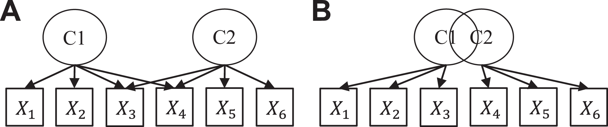
Two definitions of discriminant validity, as shown in the AMJ and JAP articles. (A) Items measure more than one construct (i.e., cross-loadings). (B) Constructs are not empirically distinct (i.e., high correlation).
These definitions were also implicitly present in other studies through the use of various statistical techniques summarized in Table 1. In the studies that assessed whether measures of two constructs were empirically distinguishable, comparison of CFA models was the most common technique, followed by calculating a correlation that was compared against a cutoff. The CFA comparison was most commonly used to assess whether two factors could be merged, but a range of other comparisons were also presented. In the correlation-based techniques, correlations were often calculated using scale scores; sometimes, correction for attenuation was used, whereas other times, estimated factor correlations were used. These correlations were evaluated by comparing the correlations with the square root of average variance extracted (AVE) or comparing their CIs against cutoffs. Some studies demonstrated that correlations were not significantly different from zero, whereas others showed that correlations were significantly different from one. In the studies that considered discriminant validity as the degree to which each item measured one construct only and not something else, various factor analysis techniques were the most commonly used, typically either evaluating the fit of the model where cross-loadings were constrained to be zero or estimating the cross-loadings and comparing their values against various cutoffs.
Techniques Used to Assess Discriminant Validity in AMJ, JAP, and ORM.
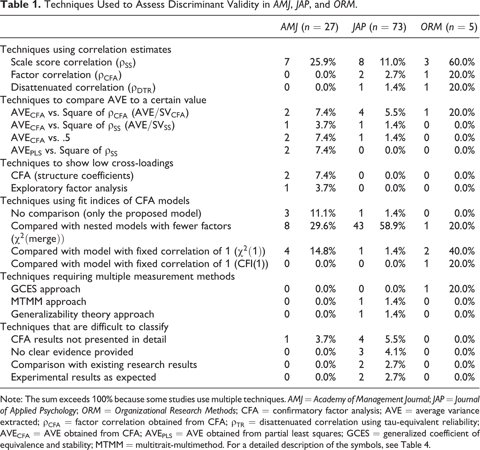
Note: The sum exceeds 100% because some studies use multiple techniques. AMJ = Academy of Management Journal; JAP = Journal of Applied Psychology; ORM = Organizational Research Methods; CFA = confirmatory factor analysis; AVE = average variance extracted;
Our review also revealed two findings that go beyond cataloging the discriminant validation techniques. First, no study evaluated discriminant validity as something that can exist to a degree but instead used the statistics to answer a yes/no type of question. Second, many techniques were used differently than originally presented. Given the diversity of how discriminant validity is conceptualized, the statistics used in its assessment, and how these statistics are interpreted, there is a clear need for a standard understanding of which technique(s) should be used and how the discriminant validity evidence produced by these techniques should be evaluated. However, to begin the evaluation of the various techniques, we must first establish a definition of discriminant validity.
Defining Discriminant Validity
Most methodological work defines discriminant validity by using a correlation but differs in what specific correlation is used, as shown in Table 2. For example, defining discriminant validity in terms of a (true) correlation between constructs implies that a discriminant validity problem cannot be addressed with better measures. In contrast, defining discriminant validity in terms of measures or estimated correlation ties it directly to particular measurement procedures. Some studies (i.e., categories 3 and 4 in Table 2) used definitions involving both constructs and measures stating that a measure should not correlate with or be affected by an unrelated construct. Moreover, there is no consensus on what kind of attribute discriminant validity is; some studies (Bagozzi & Phillips, 1982; Hamann et al., 2013; Reichardt & Coleman, 1995; J. A. Shaffer et al., 2016) define discriminant validity as a matter of degree, while others (Schmitt & Stults, 1986; Werts & Linn, 1970) define discriminant validity as a dichotomous attribute. These findings raise two important questions: (a) Why is there such diversity in the definitions? and (b) How exactly should discriminant validity be defined?
Definitions of Discriminant Validity in Existing Studies.
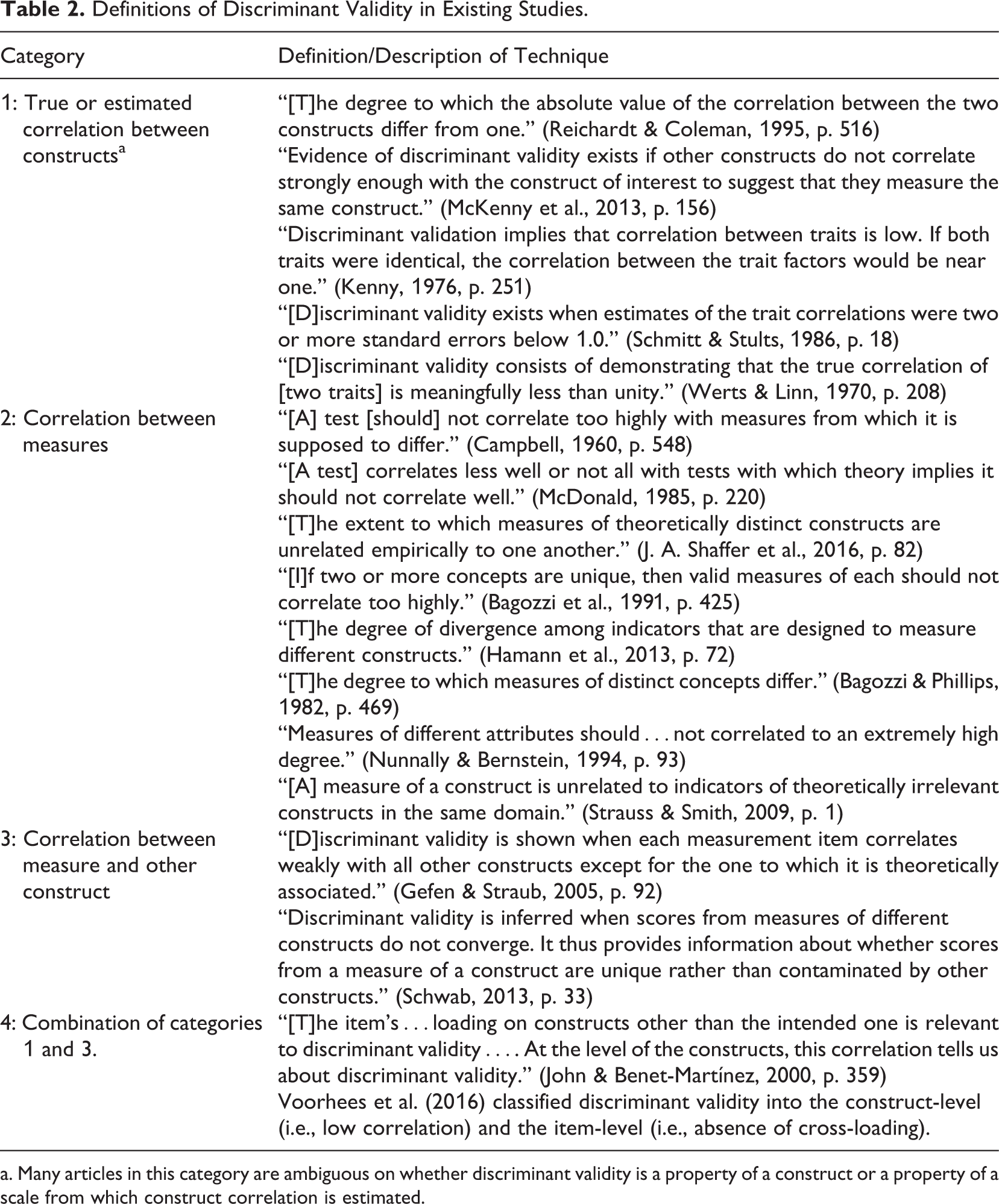
a. Many articles in this category are ambiguous on whether discriminant validity is a property of a construct or a property of a scale from which construct correlation is estimated.
Origin of the Concept of Discriminant Validity
The term “discriminant validity” was coined by Campbell and Fiske (1959), who presented a validation technique based on the long-standing idea that tests can be invalidated by too high correlations with unrelated tests (Campbell, 1960; Thorndike, 1920). However, the term was introduced without a clear definition of the concept (Reichardt & Coleman, 1995); instead, the article focuses on discriminant validation or how discriminant validity can be shown empirically using multitrait-multimethod (MTMM) matrices. The original criteria, illustrated in Table 3, were as follows: (a) two variables that measure the same trait (T1) with two different methods (M1, M2) should correlate more highly than any two variables that measure two different traits (T1, T2) with different methods (M1, M2); (b) two variables that measure the same trait (T1) with two different methods (M1, M2) should correlate more highly than any two variables that measure two different traits (T1, T2) but use the same method (M1); and (c) the pattern of correlations between variables that measure different traits (T1, T2) should be very similar across different methods (M1, M2) (Campbell & Fiske, 1959).
Multitrait-Multimethod Correlation Matrix and Original Criteria for Discriminant Validity.
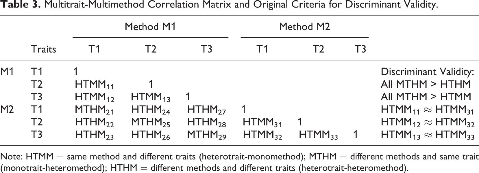
Note: HTMM = same method and different traits (heterotrait-monomethod); MTHM = different methods and same trait (monotrait-heteromethod); HTHM = different methods and different traits (heterotrait-heteromethod).
Generalizing the concept of discriminant validity outside MTMM matrices is not straightforward. Indeed, the definitions shown in Table 2 show little connections to the original MTMM matrices. A notable exception is Reichardt and Coleman (1995), who criticized the MTMM-based criteria for being dichotomous and declared that a natural (dichotomous) definition of discriminant validity outside the MTMM context would be that two measures x1 and x2 have discriminant validity if and only if x1 measures construct T1 but not T2, x2 measures T2 but not T1, and the two constructs are not perfectly correlated. They then concluded that a preferable continuous definition would be “the degree to which the absolute value of the correlation between the two constructs differs from one” (Reichardt & Coleman, 1995, p. 516). A similar interpretation was reached by McDonald (1985), who noted that two tests have discriminant validity if “the common factors are correlated, but the correlations are low enough for the factors to be regarded as distinct ‘constructs’” (p. 220).
Constructs and Measures
Discriminant validity is sometimes presented as the property of a construct (Reichardt & Coleman, 1995) and other times as the property of its measures or empirical representations constructed from those measures (McDonald, 1985). This ambiguity may stem from the broader confusion over common factors and constructs: The term “construct” refers to the concept or trait being measured, whereas a common factor is part of a statistical model estimated from data (Maraun & Gabriel, 2013). Indeed, Campbell and Fiske (1959) define validity as a feature of a test or measure, not as a property of the trait or construct being measured. In fact, if one takes the realist perspective that constructs exist independently of measurement and can be measured in multiple different ways (Chang & Cartwright, 2008), 1 it becomes clear that we cannot use an empirical procedure to define a property of a construct.
The Role of the Factor Model
Factor analysis has played a central role in articles on discriminant validation (e.g., McDonald, 1985), but it cannot serve as a basis for a definition of discriminant validity for two reasons. First, validity is a feature of a test or a measure or its interpretation (Campbell & Fiske, 1959), not of any particular statistical analysis. Moreover, discriminant validity is often presented as a property of “an item” (Table 2), implying that the concept should also be applicable in the single-item case, where factor analysis would not be applicable. Second, a factor model where each item loads on only one factor may be too constraining for applied research (Asparouhov et al., 2015; Marsh et al., 2014; Morin et al., 2017; Rodriguez et al., 2016). For example, Marsh et al. (2014) note that in psychology research, the symptoms or characteristics of different disorders commonly overlap, producing nonnegligible cross-loadings in the population. Constraining these cross-loadings to be zero can inflate the estimated factor correlations, which is problematic, particularly for discriminant validity assessment (Marsh et al., 2014). Moreover, a linear model where factors, error terms, and observed variables are all continuous (Bartholomew, 2007) is not always realistic. Indeed, a number of item response theory models have been introduced (Foster et al., 2017; Reise & Revicki, 2014) to address these scenarios and have been applied to assess discriminant validity using MTMM data (Jeon & Rijmen, 2014).
Generalized Definition of Discriminant Validity
We present a definition that does not depend on a particular model and makes it explicit that discriminant validity is a feature of a measure instead of a construct: 2 Two measures intended to measure distinct constructs have discriminant validity if the absolute value of the correlation between the measures after correcting for measurement error is low enough for the measures to be regarded as measuring distinct constructs.
This definition encompasses the early idea that even moderately high correlations between distinct measures can invalidate those measures if measurement error is present (Thorndike, 1920), which serves as the basis of discriminant validity (Campbell & Fiske, 1959). The definition can also be applied on both the scale level and the scale-item level. Consider the proposed definition in the context of the common factor model:

where


where J is a unit matrix (a matrix of ones) and
Our definition has several advantages over previous definitions shown in Table 2. First, it clearly states that discriminant validity is a feature of measures and not constructs and that it is not tied to any particular statistical test or cutoff (Schmitt, 1978; Schmitt & Stults, 1986). Second, the definition is compatible with both continuous and dichotomous interpretations, as it suggests the existence of a threshold, that is, a correlation below a certain level has no problem with discriminant validity but does not dictate a specific cutoff, thus also allowing the value of the correlation to be interpreted instead of simply tested. Third, the definition is not tied to any particular measurement process (e.g., single administration) but considers measurement error generally, thus supporting rater, transient, and other errors (Le et al., 2009; Schmidt et al., 2003). Fourth, the definition is not tied to either the individual item level or the multiple item scale level but works across both, thus unifying the category 1 and category 2 definitions of Table 2. Fifth, the definition does not confound the conceptually different questions of whether two measures measure different things (discriminant validity) and whether the items measure what they are supposed to measure and not something else (i.e., lack of cross-loadings in
This definition also supports a broad range of empirical practice: If considered on the scale level, the definition is compatible with the current tests, including the original MTMM approach (Campbell & Fiske, 1959). However, it is not limited to simple linear common factor models where each indicator loads on just one factor but rather supports any statistical technique including more complex factor structures (Asparouhov et al., 2015; Marsh et al., 2014; Morin et al., 2017; Rodriguez et al., 2016) and nonlinear models (Foster et al., 2017; Reise & Revicki, 2014) as long as these techniques can estimate correlations that are properly corrected for measurement error and supports scale-item level evaluations.
Overview of the Techniques for Assessing Discriminant Validity
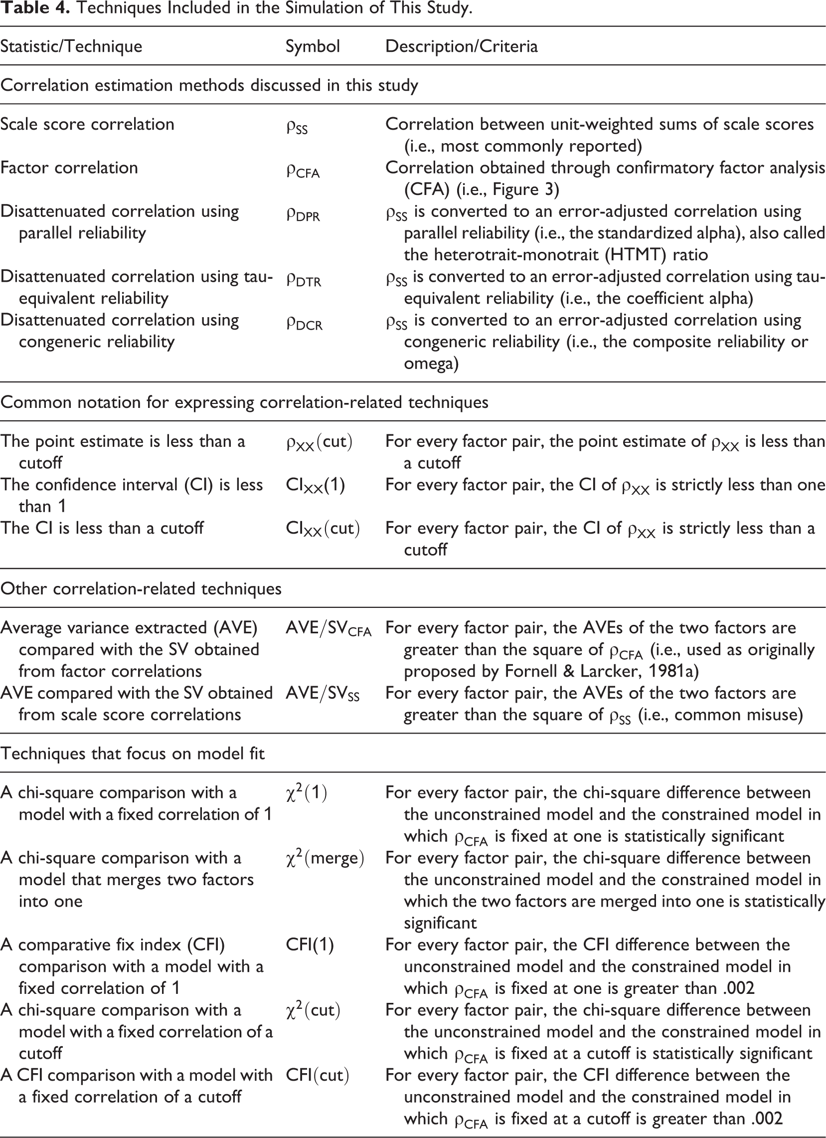
The techniques for assessing discriminant validity identified in our review can be categorized into (a) techniques that assess correlations and (b) techniques that focus on model fit assessment. The techniques and the symbols that we use for them are summarized in Table 4.
Techniques Included in the Simulation of This Study.
Techniques That Assess Correlations
There are three main ways to calculate a correlation for discriminant validity assessment: a factor analysis, a scale score correlation, and the disattenuated version of the scale score correlation. While item-level correlations or their disattenuated versions could also be applied in principle, we have seen this practice neither recommended nor used. Thus, in practice, the correlation techniques always correspond to the empirical test shown as Equation 3. Regardless of how the correlations are calculated, they are used in just two ways: either by comparing the point estimates against a cutoff (i.e., the square root of the AVE) or by checking whether the absolute value of the CI contains either zero or one. Using the cutoff of zero is clearly inappropriate as requiring that two factors be uncorrelated is not implied by the definition of discriminant validity and would limit discriminant validity assessment to the extremely rare scenario where two constructs are assumed to be (linearly) independent. We will next address the various techniques in more detail.
Factor Analysis Techniques
Factor correlations can be estimated directly either by exploratory factor analysis (EFA) or CFA, but because none of the reviewed guidelines or empirical applications reported EFA correlations, we focus on CFA. The estimation of factor correlations in a CFA is complicated by the fact by default latent variables are scaled by fixing the first indicator loadings, which produces covariances that are not correlations. Correlations (denoted
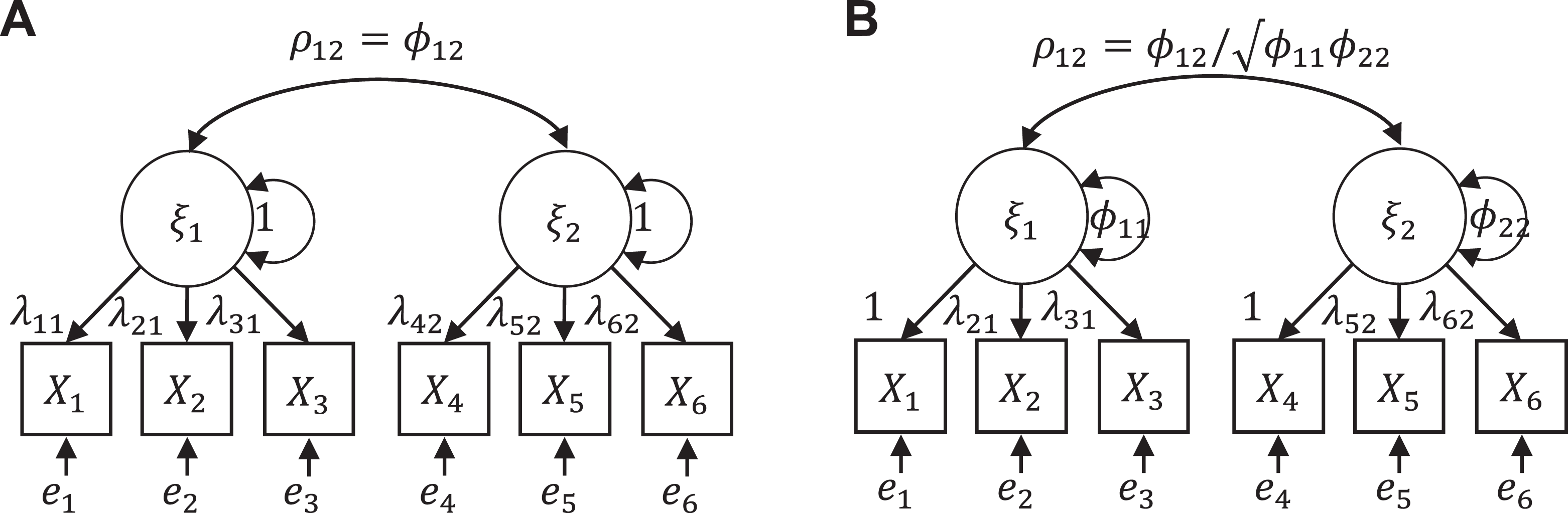
Factor correlation estimation. (A) Fixing the variances of factors to unity (i.e., not using the default option). (B) Fixing one of the loadings to unity (i.e., using the default option).
Of the correlation estimation techniques, CFA is the most flexible because it is not tied to a particular model but requires only that the model be correctly specified. Thus, cross-loadings, nonlinear factor loadings or nonnormal error terms can be included because a CFA model can also be used in the context of item response models (Foster et al., 2017), bifactor models (Rodriguez et al., 2016), exploratory SEMs (Marsh et al., 2014) or other more advanced techniques. However, these techniques tend to require larger sample sizes and advanced software and are consequently less commonly used.
Scale Score Correlations and Disattenuated Correlations
The simplest and most common way to estimate a correlation between two scales is by summing or averaging the scale items as scale scores and then taking the correlation (denoted

where the disattenuated correlation (
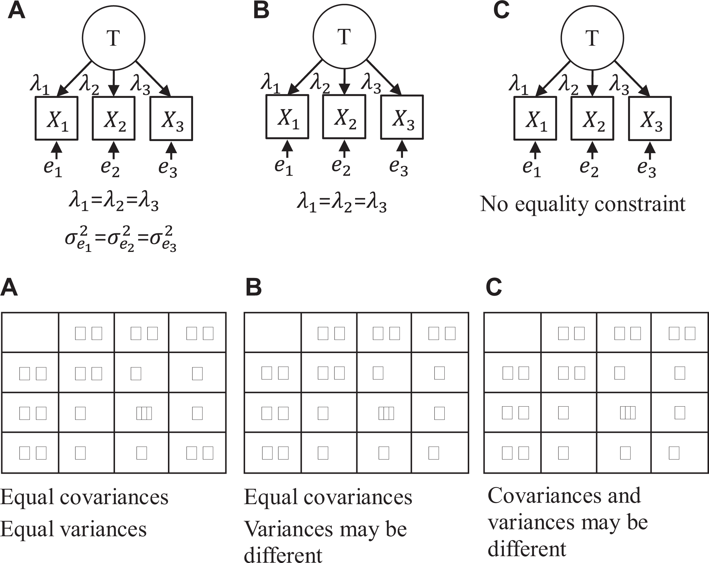
Reliability can be estimated in different ways, including test-retest reliability, interrater reliability and single-administration reliability, 7 which each provide information on different sources of measurement error (Le et al., 2009; Schmidt et al., 2003). Given our focus on single-method and one-time measurements, we address only single-administration reliability, where measurement errors are operationalized by uniqueness estimates, ignoring time and rater effects that are incalculable in these designs. The two most commonly used single-administration reliability coefficients are tau-equivalent reliability, 8 often referred to as Cronbach’s alpha, and congeneric reliability, usually called composite reliability by organizational researchers and McDonald’s omega or ω by methodologists. 9 As the names indicate, the key difference is whether we assume that the items share the same true score (tau-equivalent, B in Figure 3) or make the less constraining assumption that the items simply depend on the same latent variable but may do so to different extents (congeneric, C in Figure 3). Recent research suggests that the congeneric reliability coefficient is a safer choice because of the less stringent assumption (Cho, 2016; Cho & Kim, 2015; McNeish, 2017).
The assumptions of parallel, tau-equivalent, and congeneric reliability. (A) parallel, (B) tau-equivalent, (C) congeneric.
The reliability coefficients presented above make a unidimensionality assumption, which may not be realistic in all empirical research. While the disattenuation formula (Equation 4) is often claimed to assumes that the only source of measurement error is random noise or unreliability, the assumption is in fact more general: All variance components in the scale scores that are not due to the construct of interest are independent of the construct and measurement errors of other scale scores. This more general formulation seems to open the option of using hierarchical omega (Cho, 2016; Zinbarg et al., 2005), which assumes that the scale measures one main construct (main factor) but may also contain a number of minor factors that are assumed to be uncorrelated with the main factor. However, using hierarchical omega for disattenuation is problematic because it introduces an additional assumption that the minor factors (e.g., disturbances in the second-order factor model and group factors in the bifactor model) are also uncorrelated between two scales, which is neither applied nor tested when reliability estimates are calculated separately for both scales, as is typically the case. While the basic disattenuation formula has been extended to cases where its assumptions are violated in known ways (Wetcher-Hendricks, 2006; Zimmerman, 2007), the complexities of modeling the same set of violations in both the reliability estimates and the disattenuation equation do not seem appealing given that the factor correlation can be estimated more straightforwardly with a CFA instead.
While simple to use, the disattenuation correction is not without problems. A common criticism is that the correction can produce inadmissible correlations (i.e., greater than 1 or less than –1) (Charles, 2005; Nimon et al., 2012), but this issue is by no means a unique problem because the same can occur with a CFA. However, a CFA has three advantages over the disattenuation equation. First, CFA correlations estimated with maximum likelihood (ML) can be expected to be more efficient than multistep techniques that rely on corrections for attenuation (Charles, 2005; Muchinsky, 1996). Second, the disattenuation equation assumes that the scales are unidimensional and that all measurement errors are uncorrelated, whereas a CFA simply assumes that the model is correctly specified and identified. Third, calculating the CIs for a disattenuated correlation is complicated (Oberski & Satorra, 2013). However, this final concern can be alleviated to some extent through the use of bootstrap CIs (Henseler et al., 2015); in particular, the bias-corrected and accelerated (BCa) technique has been shown to work well for this particular problem (Padilla & Veprinsky, 2012, 2014).
AVE/SV or Fornell-Larcker Criterion
While commonly used, the AVE statistic has been rarely discussed by methodological research and, consequently, is poorly understood. 10 One source of confusion is the similarity between the formula for AVE and that of congeneric reliability (Fornell & Larcker, 1981a):
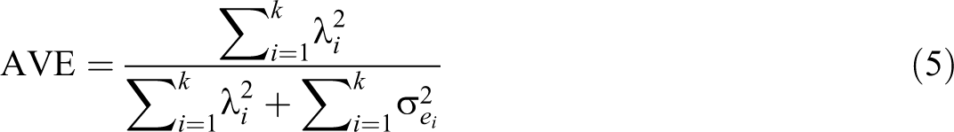
The meaning of AVE becomes more apparent if we rewrite the original equation as:
where
Fornell and Larcker (1981a) presented a decision rule that discriminant validity holds for two scales if the AVEs for both are higher than the squared factor correlation between the scales. We refer to this rule as AVE/SV because the squared correlation quantifies shared variance (SV; Henseler et al., 2015). Because a factor correlation corrects for measurement error, the AVE/SV comparison is similar to comparing the left-hand side of Equation 3 against the right-hand side of Equation 2. Therefore, AVE/SV has a high false positive rate, indicating a discriminant validity problem under conditions where most researchers would not consider one to exist, as indicated by A in Figure 4. This tendency has been taken as evidence that AVE/SV is “a very conservative test” (Voorhees et al., 2016, p. 124), whereas the test is simply severely biased.
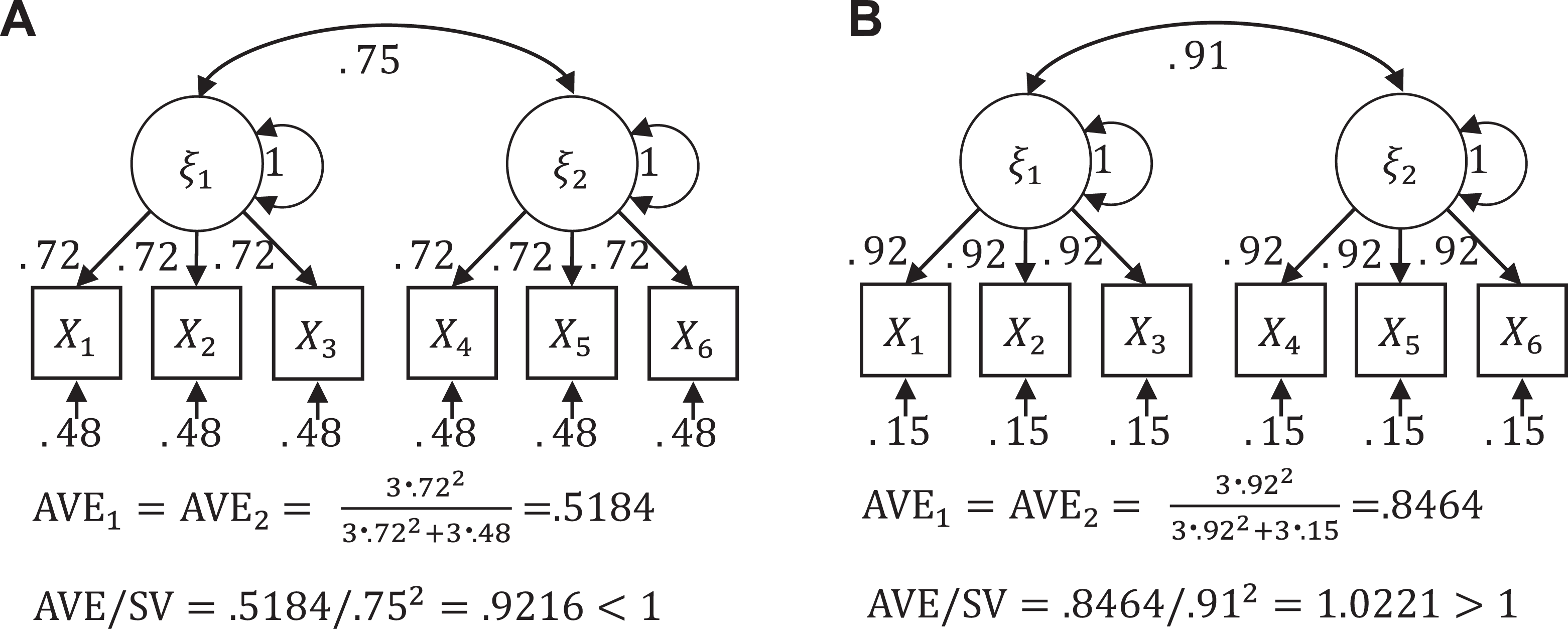
The inappropriateness of the AVE as an index of discriminant validity. (A) despite high discriminant validity, the AVE/SV criterion fails, (B) despite low discriminant validity, the AVE/SV criterion passes.
In applied research, the AVE/SV criterion rarely shows a discriminant validity problem because it is commonly misapplied. The most common misapplication is to compare the AVE values with the square of the scale score correlation, not the square of the factor correlation (Voorhees et al., 2016). Another misuse is to compare AVEs against the .5 rule-of-thumb cutoff, which Fornell and Larcker (1981a) presented as a convergent validity criterion. Other misuses are that only one of the two AVE values or the average of the two AVE values should be greater than the SV (Farrell, 2010; Henseler et al., 2015). The original criterion is that both AVE values must be greater than the SV. Finally, the AVE statistic is sometimes calculated from a partial least squares analysis (AVEPLS), which overestimates indicator reliabilities and thus cannot detect even the most serious problems (Rönkkö & Evermann, 2013).
Heterotrait-Monotrait Ratio (HTMT)
The heterotrait-monotrait (HTMT) ratio was recently introduced in marketing (Henseler et al., 2015) and is being adopted in other disciplines as well (Kuppelwieser et al., 2019). While Henseler et al. (2015) motivate HTMT based on the original MTMM approach (Campbell & Fiske, 1959), this index is actually neither new nor directly based on the MTMM approach. The original version of the HTMT equation is fairly complex, but to make its meaning more apparent, it can be simplified as follows:

where
Because the
Model Fit Comparison Techniques
Model comparison techniques involve comparing the original model against a model where a factor correlation is fixed to a value high enough to be considered a discriminant validity problem. Their general idea is that if the two models fit equally well, the model with a discriminant validity problem is plausible, and thus, there is a problem. The most common constraints are that (a) two factors are fixed to be correlated at 1 (i.e., A in Figure 5) or (b) two factors are merged into one factor (i.e., C in Figure 5), thus reducing their number by one.
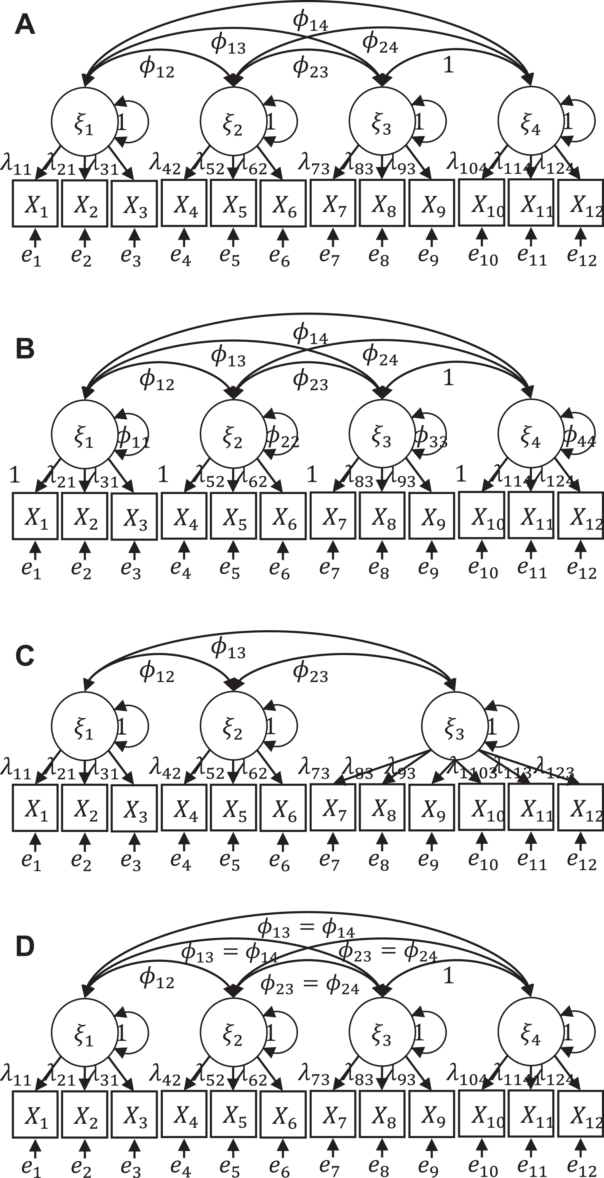
(A) constrained model for χ2(1), (B) common misuse of χ2(1), (C) constrained model for χ2(merge), (D) model equivalent to C.
The key advantage of these techniques is that they provide a test statistic and a p-value. However, this also has the disadvantage that it steers a researcher toward making yes/no decisions instead of assessing the degree to which discriminant validity holds in the data. Compared to correlation-based techniques, where a single CFA model provides all the estimates required for discriminant validity assessment, model comparison techniques require more work because a potentially large number of comparisons must be managed. 11 We next assess the various model comparison techniques presented and used in the literature.
In the
The second issue is that some articles suggest that the significance level of the
The third issue is that the
The fourth and final issue is that the
CFI(1)
To address the issue that the
The idea behind using ΔCFI in measurement invariance assessment is that the degrees of freedom of the invariance hypothesis depend on the model complexity, and the CFI index and consequently ΔCFI are less affected by this than the

instead of using the .95 percentile from the
Changing the test statistic—or equivalently the cutoff value—is an ultimately illogical solution because the problem with the
and
The lack of a perfect correlation between two latent variables is ultimately rarely of interest, and thus, it is more logical to use a null hypothesis that covers an interval (e.g.,
and Other Comparisons Against Models with Fewer Factors
Many studies assess discriminant validity by comparing the hypothesized model with a model with fewer factors. This is typically done by merging two factors (i.e., C in Figure 5), and we refer to the associated nested model comparison as
As with the other techniques, various misconceptions and misuses are found among empirical studies. The most common misuse is to include unnecessary comparisons, for example, by testing alternative models with two or more factors less than the hypothesized model. Another common misuse is to omit some necessary comparisons, for example, by comparing only some alternative models, instead of comparing all possible alternative models with one factor less than the original model.
Single Model Fit Techniques
Discriminant validity has also been assessed by inspecting the fit of a single model without comparing against another model. These techniques fall into two classes: those that inspect the factor loadings and those that assess the overall model fit.
Cross-Loadings
Cross-loadings indicate a relationship between an indicator and a factor other than the main factor on which the indicator loads. Beyond this definition, the term can refer to two distinct concepts, factor pattern coefficients or factor structure coefficients (see Table 5), and has been confusingly used with both meanings in the discriminant validity literature. 15 Structure coefficients are correlations between items and factors, so their values are constrained to be between –1 and 1. Pattern coefficients, on the other hand, are analogous to (standardized) coefficients in regression analysis and are directional (Thompson & Daniel, 1996). Structure coefficients are not directly estimated as part of a factor analysis; instead, they are calculated based on the pattern coefficients and factor correlations. If the factors are rotated orthogonally (e.g., Varimax) or are otherwise constrained to be uncorrelated, the pattern coefficients and structure coefficients are identical (Henson & Roberts, 2006). However, the use of uncorrelated factors can rarely be justified (Fabrigar et al., 1999), which means that, in most cases, pattern and structure coefficients are not equal.
Factor Pattern Coefficients, Correlations, and Structure Coefficients.
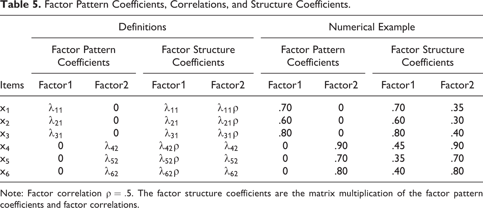
Note: Factor correlation
While both the empirical criteria shown in Equation 2 and Equation 3 contain pattern coefficients, assessing discriminant validity based on loadings is problematic. First, these comparisons involve assessing a single item or scale at a time, which is incompatible with the idea that discriminant validity is a feature of a measure pair. Second, pattern coefficients do not provide any information on the correlation between two scales, and structure coefficients are an indirect measure of the correlation at best. 16 Third, while the various guidelines differ in how loadings should be interpreted (Henseler et al., 2015; Straub et al., 2004; Thompson, 1997), they all share the features of relying mostly on authors’ intuition instead of theoretical reasoning or empirical evidence. In summary, these techniques fall into the rules of thumb category and cannot be recommended.
Single-Model fit
The final set of techniques is those that assess the single-model fit of a CFA model. A CFA model can fit the data poorly if there are unmodeled loadings (pattern coefficients), omitted factors, or error correlations in the data, none of which are directly related to discriminant validity. While some of the model fit indices do depend on factor correlations, they do so only weakly and indirectly (Kline, 2011, chap. 8). Thus, while a well-fitting factor model is an important assumption (either implicitly—e.g., the various
Summary: Under What Conditions Is Each Technique Useful?
Our review of the literature provides several conclusions. Overall,
Monte Carlo Simulations
We will next compare the various discriminant validity assessment techniques in a Monte Carlo simulation with regard to their effectiveness in two common tasks: (a) quantifying the degree to which discriminant validity can be a problem and (b) making a dichotomous decision on whether discriminant validity is a problem in the population. For statistics with meaningful interpretations, we assessed the bias and variance of the statistic and the validity of the CIs. For the dichotomous decision, we set .85, .9, .95, and 1 as cutoffs and estimated the Type I error (i.e., false positive) and Type II error (i.e., false negative) rates for the conclusion that the factor correlation was at least at the cutoff value in the population.
Simulation Design
For simplicity, we followed the design used by Voorhees et al. (2016) and generated data from a three-factor model. We assessed the discriminant validity of the first two factors, varying their correlation as an experimental condition. Voorhees et al. (2016) used only two factor correlation levels, .75 and .9. We wanted a broader range from low levels where discriminant validity is unlikely to be a problem up to perfect correlation, so we used six levels: .5, .6, .7, .8, .9, and 1. The third factor was always correlated at .5 with the first two factors. The number of items was varied at 3, 6, and 9, and factor loadings were set to [0.9,0.8,0.8], [0.8,0.7,0.7], [0.5,0.4,0.4], [0.9,0.6,0.3], and [0.8, 0.8, 0.8]. For the six- and nine-item scenarios, each factor loading value was used multiple times. All factors had unit variances in the population, and we scaled the error variances so that the population variances of the items were one. Cross-loadings (in the pattern coefficients) were either 0, 1, or 2. This condition was implemented following the approach by Voorhees et al. (2016); in the cross-loading condition, either the first or first two indicators of the second latent variable also loaded on the first latent variable. The same value was used for both loadings, and the values were scaled down from their original values so that the factors always explained the same amount of variance in the indicators. In the six- and nine-item conditions, the number of cross-loaded items was scaled up accordingly. Sample size was the final design factor and varied at 50, 100, 250, and 1,000. The full factorial (6 × 3 × 5 × 3 × 4) simulation was implemented with the R statistical programming environment using 1,000 replications for each cell. We estimated the factor models with the lavaan package (Rosseel, 2012) and used semTools to calculate the reliability indices (Jorgensen et al., 2020). The full simulation code is available in Online Supplement 2, and the full set of simulation results at the design level can be found in Online Supplement 3.
Correlation Estimates and Their Confidence Intervals
We first focus on the scenarios where the factor model was correctly specified (i.e., there were no cross-loadings). Because
Because the pattern of results is very similar for correlations and their confidence intervals, we present both sets of results together. Table 6 shows the correlation estimates by sample size, number of items, and factor loading conditions. Table 7 shows the coverage and the balance of the CIs by sample size and selected values of loading condition, omitting
Correlation Estimates by Sample Size, Number of Items, and Loadings.
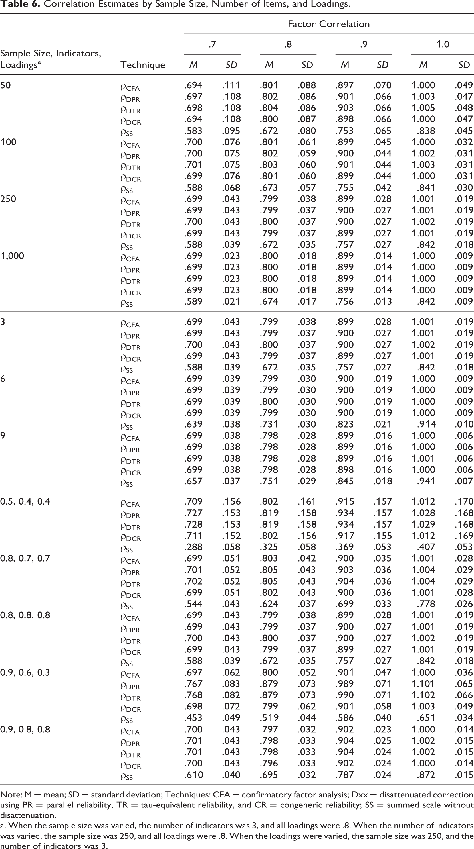
Note: M = mean; SD = standard deviation; Techniques: CFA = confirmatory factor analysis; Dxx = disattenuated correction using PR = parallel reliability, TR = tau-equivalent reliability, and CR = congeneric reliability; SS = summed scale without disattenuation.
a. When the sample size was varied, the number of indicators was 3, and all loadings were .8. When the number of indicators was varied, the sample size was 250, and all loadings were .8. When the loadings were varied, the sample size was 250, and the number of indicators was 3.
Coverage and Balance of 95% Confidence Intervals by Loadings and Sample Size.
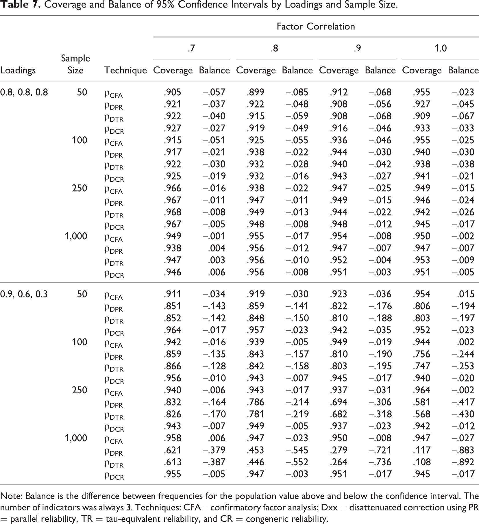
Note: Balance is the difference between frequencies for the population value above and below the confidence interval. The number of indicators was always 3. Techniques: CFA= confirmatory factor analysis; Dxx = disattenuated correction using PR = parallel reliability, TR = tau-equivalent reliability, and CR = congeneric reliability.
The first set of rows in Table 6 shows the effects of sample size. Scale score correlation
The third set of rows in Table 6 demonstrates the effects of varying the factor loadings. When the factor loadings were equal (all at .8), the performance of CFA and all disattenuation techniques was identical, which was expected, as explained above. Table 7 shows that in this condition, the confidence intervals of all techniques performed reasonably well. The balance statistics were all negative, indicating that when the population value was outside the CI, it was generally more frequently below the lower limit of the interval than above the upper limit. In other words, all CIs were slightly positively biased. This effect and the general undercoverage of the CIs were most pronounced in small samples.
When the loadings varied,
In summary, Table 6 and Table 7 show that the best-performing correlation estimate was
Inference Against a Cutoff
Our main results concern inference against a cutoff and are relevant when a researcher wants to make a yes/no decision about discriminant validity. We start by assessing the performance of the techniques that can be thought of as tests of a perfect correlation or as rules of thumb. Because the differences between
Table 8 clearly shows that some of the techniques have either unacceptably low power or a false positive rate that is too high to be considered useful. Techniques that directly compare the point estimates of correlations with a cutoff (i.e.,
The various model comparisons and CIs performed better. Among the three methods of model comparison (CFI(1),
Another interesting finding is that although
The performance of the CIs (
Detection Rates of the Discriminant Validity Problem as a Perfect Correlation by Technique.
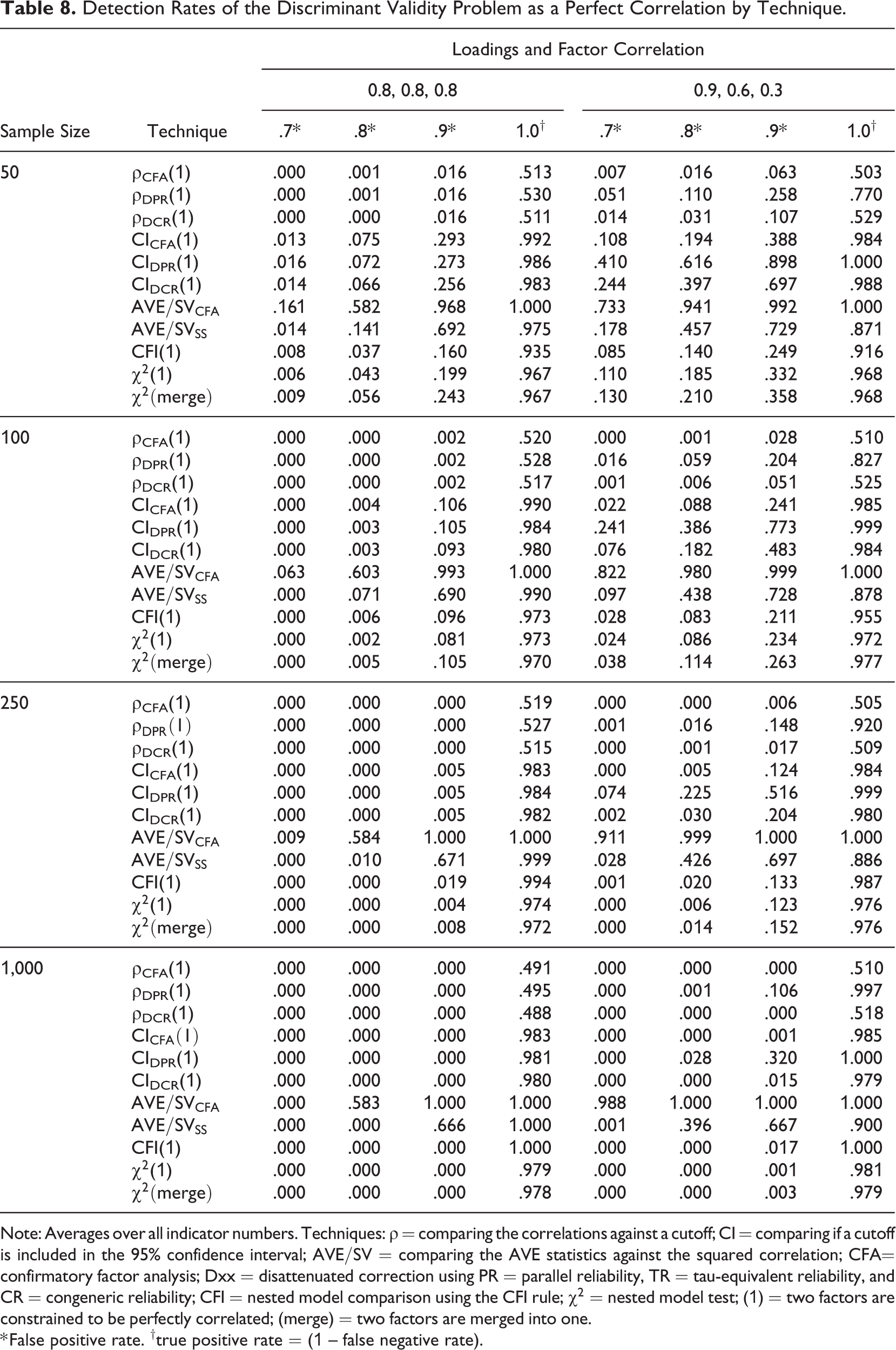
Note: Averages over all indicator numbers. Techniques:
* False positive rate. †true positive rate = (1 – false negative rate).
Table 9 considers cutoffs other than 1, using values of .85, .90, and .95 that are sometimes recommended in the literature, showing results that are consistent with those of the previous tables. The techniques that compared the CI against a cutoff (i.e.,
Detection Rates by Technique Using Alternative Cutoffs.
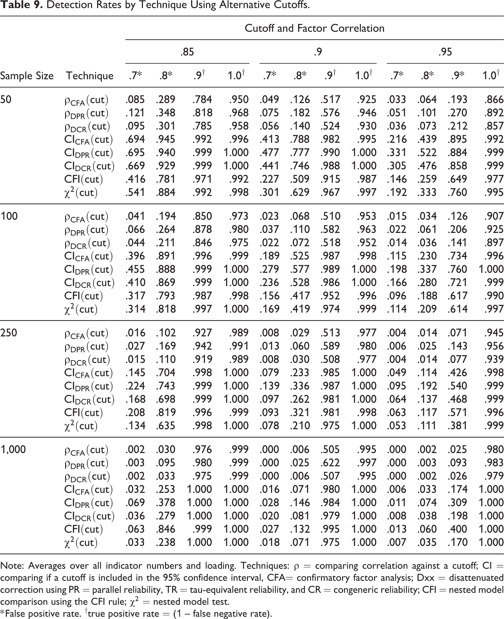
Note: Averages over all indicator numbers and loading. Techniques:
* False positive rate. †true positive rate = (1 – false negative rate).
Effects of Model Misspecification
We now turn to the cross-loading conditions to assess the robustness of the techniques when the assumption of no cross-loadings is violated. The results shown in Table 10 show that all estimates become biased toward 1.
Mean Correlation Estimate Under Model Misspecification.
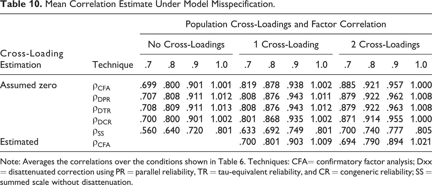
Note: Averages the correlations over the conditions shown in Table 6. Techniques: CFA= confirmatory factor analysis; Dxx = disattenuated correction using PR = parallel reliability, TR = tau-equivalent reliability, and CR = congeneric reliability; SS = summed scale without disattenuation.
Detection Rates by Technique Using Alternative Cutoffs Under Model Misspecification.
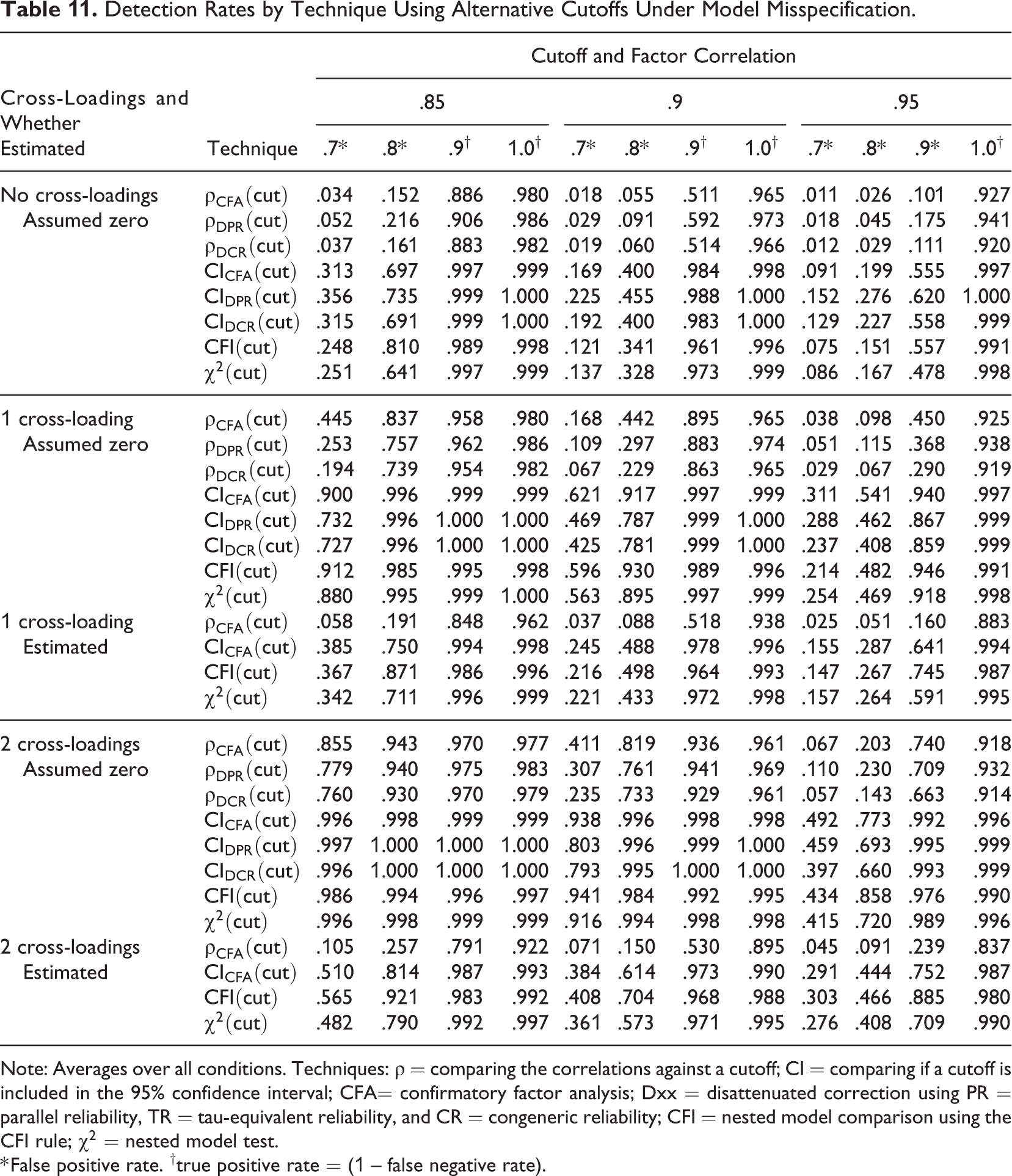
Note: Averages over all conditions. Techniques:
* False positive rate. †true positive rate = (1 – false negative rate).
In the cross-loading conditions, we also estimated a correctly specified CFA model in which the cross-loadings were estimated. Table 10 shows that the mean estimate was largely unaffected, but the variance of the estimates (not reported in the table) increased because of the increased model complexity. This effect is seen in Table 11, where the pattern of results for CFA models was largely similar between the cross-loading conditions, but the presence of cross-loadings increased the false positive rate. This result is easiest to understand in the context of
The cross-loading results underline the importance of observing the assumptions of the techniques and that not doing so may lead to incorrect inference. However, two conclusions that are new to discriminant validity literature can be drawn: First, the lack of cross-loadings in the population (i.e., factorial validity) is not a strict prerequisite for discriminant validity assessment as long as the cross-loadings are modeled appropriately. Second, while the lack of factorial validity can lead scale-item pairs to have complete lack of discriminant validity (see Equation 2), this does not always invalidate scale-level discriminant validity (see Equation 3) as long as this is properly modeled.
Discussion
The original meaning of the term “discriminant validity” was tied to MTMM matrices, but the term has since evolved to mean a lack of a perfect or excessively high correlation between two measures after considering measurement error. We provided a comprehensive review of the various discriminant validity techniques and presented a simulation study assessing their effectiveness. There are several issues that warrant discussion.
Contradictions With Prior Studies
Our simulation results clearly contradict two important conclusions drawn in the recent discriminant validity literature, and these contradictions warrant explanations. First, Henseler et al. (2015) and Voorhees et al. (2016) strongly recommend
Second, our results also challenge J. A. Shaffer et al.’s (2016) recommendation that discriminant validity should be tested by a CFI comparison between two nested models (CFI(1)). The reason for this contradiction is that their recommendation is based on the assumption that if the CFI difference works well for measurement invariance assessment, it should also work well when discriminant validity assessment. The assumption appears to be invalid as it ignores an important difference between these uses: Whereas the degrees of freedom of an invariance test scale roughly linearly with the number of indicators, the degrees of freedom in CFI(1) are always one.
Magnitude of the Discriminant Validity Correlations
In the discriminant validity literature, high correlations between scales or scale items are considered problematic. However, the literature generally has not addressed what is high enough beyond giving rule of thumb cutoffs (e.g., 85). Our definition of discriminant validity suggests that the magnitude of the estimated correlation depends on the correlation between the constructs, the measurement process, and the particular sample, each of which has different implications on what level should be considered high. To warn against mechanical use, we present a scenario where high correlation does not invalidate measurement and a scenario where low correlation between measures does not mean that they measure distinct constructs.
A large correlation does not always mean a discriminant validity problem if one is expected based on theory or prior empirical observations. For example, the correlation between biological sex and gender identity can exceed .99 in the population. 17 However, both variables are clearly distinct: sex is a biological property with clear observable markers, whereas gender identity is a psychological construct. These two variables also have different causes and consequences (American Psychological Association, 2015), so studies that attempt to measure both can lead to useful policy implications. In cases such as this where the constructs are well defined, large correlations should be tolerated when expected based on theory and prior empirical results. Of course, large samples and precise measurement would be required to ensure that the constructs can be distinguished empirically (i.e., are empirically distinct).
A small or moderate correlation (after correcting for measurement error) does not always mean that two measures measure concepts that are distinct. For example, consider two thermometers that measure the same temperature, yet one is limited to measuring only temperatures above freezing, whereas the other can measure only temperatures below freezing. While both measure the same quantity, they are correlated only by approximately .45 because the temperature would always be out of the range of one of the thermometers that would consequently display zero centigrade. 18 In the social sciences, a well-known example is the measurement of happiness and sadness, two constructs that can be thought of as opposite poles of mood (D. P. Green et al., 1993; Tay & Jebb, 2018). Consequently, any evaluation of the discriminant validity of scales measuring two related constructs must precede the theoretical consideration of the existence of a common continuum. If this is the case, the typical discriminant validity assessment techniques that are the focus of our article are not directly applicable, but other techniques are needed (Tay & Jebb, 2018).
As the two examples show, a moderately small correlation between measures does not always imply that two constructs are distinct, and a high correlation does not imply that they are not. Like any validity assessment, discriminant validity assessment requires consideration of context, possibly relevant theory, and empirical results and cannot be reduced to a simple statistical test and a cutoff no matter how sophisticated. These considerations highlight the usefulness of the continuous interpretation of discriminant validity evidence.
On Choosing a Technique and a Cutoff
While a general set of statistics and cutoffs that is applicable to all research scenarios cannot exist, we believe that establishing some standards is useful. Based on our study,
Equally important to choosing a technique is the choice of a cutoff if the technique requires one. Of the recent simulation studies, Henseler et al. (2015) suggested cutoffs of .85 and .9 based on prior literature (e.g., Kline, 2011). Voorhees et al. (2016) considered the false positive and false negative rates of the techniques used in their study and concluded that the cutoff of .85 had the best balance of high power and an acceptable Type I error rate. However, as explained in Online Supplement 5, such conclusions are to a large part simply artifacts of the simulation design. In sum, it seems that deriving an ideal cutoff through simulation results is meaningless and must be established by consensus among the field.
Empirical studies seem to agree that correlations greater than .9 indicate a problem and that correlations less than .8 indicate the lack of a problem. For example, Le et al. (2010) diagnosed a discriminant validity problem between job satisfaction and organizational commitment based on a correlation of .91, and Mathieu and Farr (1991) declared no problem of discriminant validity between the same variables on the basis of a correlation of .78. However, mixed judgments were made about the correlation values between .8 and .9. Lucas et al. (1996) acknowledged discriminant validity between self-esteem and optimism based on
Sources of Error Other Than the Random Error and Item-Specific Factor Error
Our focus on the common scenario of single-method and one-time measurements limits the researcher to techniques that operationalize measurement error as item uniqueness either directly (e.g., CFA) or indirectly (e.g.,
A Guideline for Assessing Discriminant Validity
From a Cutoff to a Classification System
While many articles about discriminant validity consider it as a matter of degree (e.g., “the extent to…”) instead of a yes/no issue (e.g., “whether…”), most guidelines on evaluation techniques, including Campbell and Fiske’s (1959) original proposal, focus on making a dichotomous judgment as to whether a study has a discriminant validity problem (B in Figure 6). This inconsistency might be an outcome of researchers favoring cutoffs for their simplicity, or it may reflect the fact that after calculating a discriminant validity statistic, researchers must decide whether further analysis and interpretation is required. This practice also fits the dictionary meaning of evaluation, which is not simply calculating and reporting a number but rather dividing the object into several qualitative categories based on the number, thus requiring the use of cutoffs, although these do not need to be the same in every study.
To move the field toward discriminant validity evaluation, we propose a system consisting of several cutoffs instead of a single one. Discriminant validity is a continuous function of correlation values (C in Figure 6), but because of practical needs, correlations are classified into discrete categories indicating different degrees of a problem (D in Figure 6). Similar classifications are used in other fields to characterize essentially continuous phenomena: Consider a doctor’s diagnosis of hypertension. In the past, everyone was divided into two categories of normal and patient, but now hypertension is classified into several levels. That is, patients with hypertension are further subdivided into three stages according to their blood pressure level, and each level is associated with different treatments.
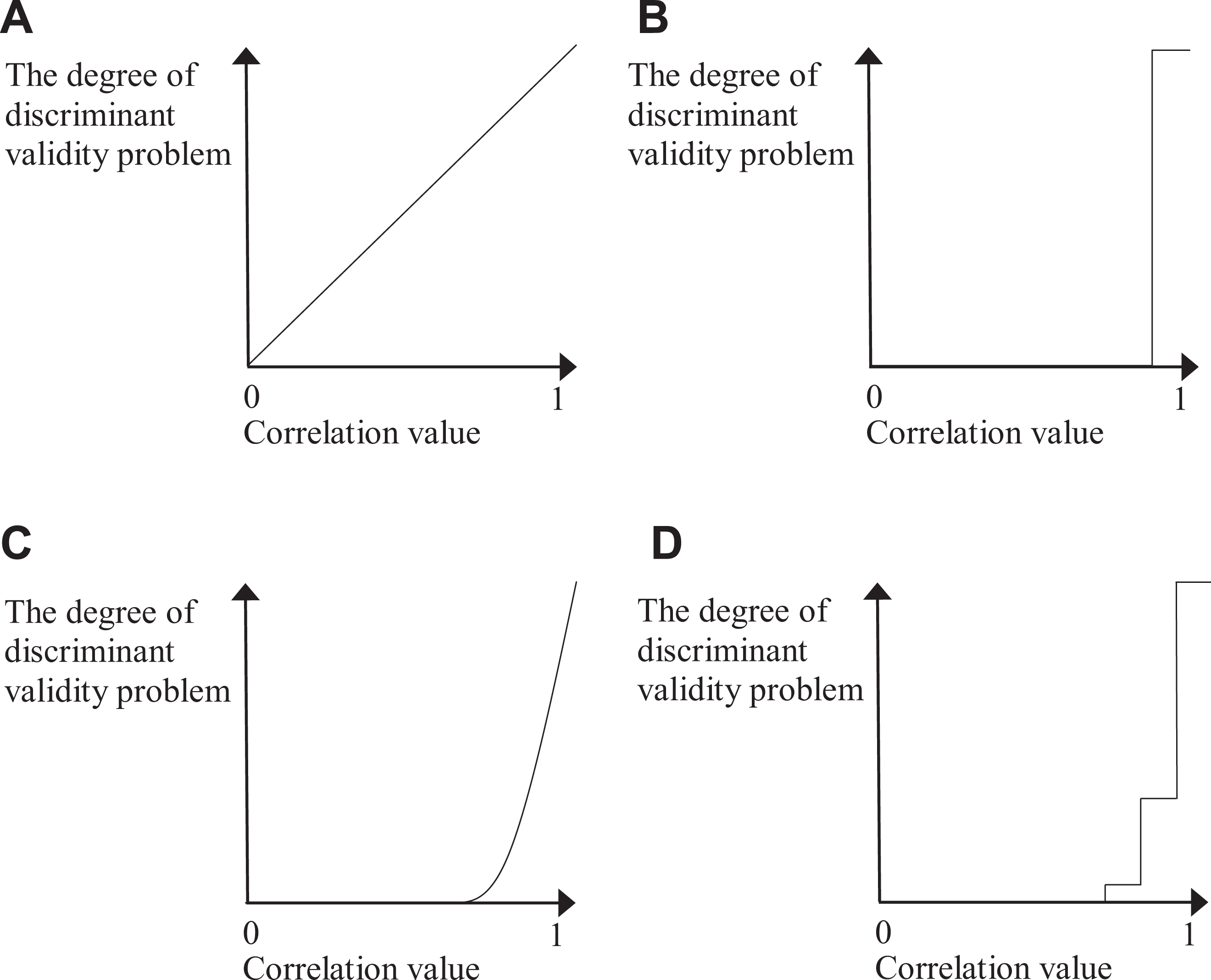
Relationship between correlation values and the problem of discriminant validity. (A) Linear model (implied by existing definitions), (B) Dichotomous model (existing techniques), (C) Threshold model (implied by the definition of this study), (D) Step model (proposed evaluation technique).
Table 12 shows the classification system we propose. We emphasize that these are guideline that can be adjusted case-by-case if warranted by theoretical understanding of the two constructs and measures, not strict rules that should always be followed. Based on our review, correlations below .8 were seldom considered problematic, and this is thus used as the cutoff for the first class, “No problem,” which strictly speaking is not a proof of no problem, just no evidence of a problem. When correlations fall into this class, researchers can simply declare that they did not find any evidence of a discriminant validity problem. The next three steps are referred to as Marginal, Moderate, and Severe problems, respectively. The Severe problem is the most straightforward: two items or scales cannot be distinguished empirically, and researchers should rethink their concept definitions, measurement, or both. In empirical applications, the correlation level of .9 was nearly universally interpreted as a problem, and we therefore use this level as a cutoff between the Marginal and Moderate cases. In both cases, the high correlation should be acknowledged, and its possible cause should be discussed. In the Marginal case, the interpretation of the scales as representations of distinct constructs is probably safe. In the Moderate case, additional evidence from prior studies using the same constructs and/or measures should be checked before interpretation of the results to ensure that the high correlation is not a systematic problem with the constructs or scales.
Proposed Classification and Cutoffs.
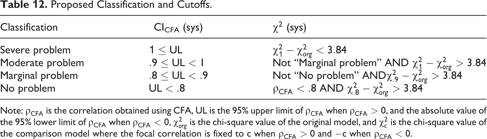
Note:
How to Implement the Proposed Techniques
The proposed classification system should be applied with CICFA(cut) and
Implementing
Online Supplement 4 provides a tutorial on how to implement the techniques described in this article using AMOS, LISREL, Mplus, R, and Stata. Because implementing a sequence of comparisons is cumbersome and prone to mistakes, we have contributed a function that automates the
What to Do When Discriminant Validity Fails?
If problematically high correlations are observed, their sources must be identified. We propose a three-step process: First, suspect conceptual redundancy. We suggest starting by following the guidelines by J. A. Shaffer et al. (2016) and Podsakoff et al. (2016) for assessing the conceptual distinctiveness of the constructs (see also M. S. Krause, 2012). If two constructs are found to overlap conceptually, researchers should seriously consider dropping one of the constructs to avoid the confusion caused by using two different labels for the same concept or phenomenon (J. A. Shaffer et al., 2016).
Second, scrutinize the measurement model. An unexpectedly high correlation estimate can indicate a failure of model assumptions, as demonstrated by our results of misspecified models. Check the
Third, collect different data. If conceptual overlap and measurement model issues have been ruled out, the discriminant validity problem can be reduced to a multicollinearity problem. For example, if one wants to study the effects of hair color and gender on intelligence but samples only blonde men and dark-haired women, hair color and gender are not empirically distinguishable, although they are both conceptually distinct and virtually uncorrelated in the broader population. This can occur either because of a systematic error in the sampling design or due to chance in small samples. If a systematic error can be ruled out, the most effective remedy is to collect more data. Alternatively, the data can be used as such, in which case large standard errors will indicate that little can be said about the relative effects of the two variables, or the two variables can be combined as an index (Wooldridge, 2013, pp. 94–98). If a researcher chooses to interpret results, he or she should clearly explain why the large correlation between the latent variables (e.g., >.9) is not a problem in the particular study.
Reporting
We also provide a few guidelines for improved reporting. First, researchers should clearly indicate what they are assessing when assessing discriminant validity by stating, for example, that “We addressed discriminant validity (whether two scales are empirically distinct).” Second, the correlation tables, which are ubiquitous in organizational research, are in most cases calculated with scale scores or other observed variables. However, most studies use only the lower triangle of the table, leaving the other half empty (AMJ 93.6%, JAP 83.1%). This practice is a waste of scarce resources, and we suggest that this space should be used for the latent correlation estimates, which serve as continuous discriminant validity evidence. Third, if nested model comparisons (e.g.,
Concluding Remarks
There is no shortage of various statistical techniques for evaluating discriminant validity. Such an abundance of techniques is positive if techniques have different advantages, and they are purposefully selected based on their fit with the research scenario. The current state of the discriminant validity literature and research practice suggests that this is not the case. Instead, it appears that many of the techniques have been introduced without sufficient testing and, consequently, are applied haphazardly. Because direct criticism of existing techniques is often avoided, there appears to be a tendency in which new techniques continue to be added without clarifying the problems of previously used techniques. This technique proliferation causes confusion and misuse. This study draws an unambiguous conclusion about which method is best for assessing discriminant validity and which methods are inappropriate. We hope that the article will help readers discriminate valid techniques from those that are not.
Supplemental Material
Supplemental Material, Online_supplement_1_-_Chi2(1)_scaling_example - An Updated Guideline for Assessing Discriminant Validity
Supplemental Material, Online_supplement_1_-_Chi2(1)_scaling_example for An Updated Guideline for Assessing Discriminant Validity by Mikko Rönkkö and Eunseong Cho in Organizational Research Methods
Supplemental Material
Supplemental Material, Online_supplement_2_-_Full_simulation_code - An Updated Guideline for Assessing Discriminant Validity
Supplemental Material, Online_supplement_2_-_Full_simulation_code for An Updated Guideline for Assessing Discriminant Validity by Mikko Rönkkö and Eunseong Cho in Organizational Research Methods
Supplemental Material
Supplemental Material, Online_supplement_3_-_Full_simulation_results - An Updated Guideline for Assessing Discriminant Validity
Supplemental Material, Online_supplement_3_-_Full_simulation_results for An Updated Guideline for Assessing Discriminant Validity by Mikko Rönkkö and Eunseong Cho in Organizational Research Methods
Supplemental Material
Supplemental Material, Online_supplement_4_-_Tutorial_on_calculations - An Updated Guideline for Assessing Discriminant Validity
Supplemental Material, Online_supplement_4_-_Tutorial_on_calculations for An Updated Guideline for Assessing Discriminant Validity by Mikko Rönkkö and Eunseong Cho in Organizational Research Methods
Supplemental Material
Supplemental Material, Online_supplement_5_-_Deriving_a_cutoff_based_on_simulation_results - An Updated Guideline for Assessing Discriminant Validity
Supplemental Material, Online_supplement_5_-_Deriving_a_cutoff_based_on_simulation_results for An Updated Guideline for Assessing Discriminant Validity by Mikko Rönkkö and Eunseong Cho in Organizational Research Methods
Footnotes
Appendix: Proofs
Acknowledgments
We are deeply grateful to Louis Tay, associate editor, and two anonymous reviewers for their invaluable guidance and constructive comments. We acknowledge the computational resources provided by the Aalto Science-IT project.
Declaration of Conflicting Interests
The author(s) declared no potential conflicts of interest with respect to the research, authorship, and/or publication of this article.
Funding
The author(s) disclosed receipt of the following financial support for the research, authorship, and/or publication of this article: This research was supported in part by a grant from the Academy of Finland (Grant 311309) and the Research Grant of Kwangwoon University in 2019.
Notes
References
Supplementary Material
Please find the following supplemental material available below.
For Open Access articles published under a Creative Commons License, all supplemental material carries the same license as the article it is associated with.
For non-Open Access articles published, all supplemental material carries a non-exclusive license, and permission requests for re-use of supplemental material or any part of supplemental material shall be sent directly to the copyright owner as specified in the copyright notice associated with the article.