
Abstract
Theoretical “necessary but not sufficient” statements are common in the organizational sciences. Traditional data analyses approaches (e.g., correlation or multiple regression) are not appropriate for testing or inducing such statements. This article proposes necessary condition analysis (NCA) as a general and straightforward methodology for identifying necessary conditions in data sets. The article presents the logic and methodology of necessary but not sufficient contributions of organizational determinants (e.g., events, characteristics, resources, efforts) to a desired outcome (e.g., good performance). A necessary determinant must be present for achieving an outcome, but its presence is not sufficient to obtain that outcome. Without the necessary condition, there is guaranteed failure, which cannot be compensated by other determinants of the outcome. This logic and its related methodology are fundamentally different from the traditional sufficiency-based logic and methodology. Practical recommendations and free software are offered to support researchers to apply NCA.
According to David Hume’s (1777) philosophy of causation: We may define a cause to be an object, followed by another, and where all the objects, similar to the first, are followed by objects, similar to the second. Or in other words, where, if the first had not been, the second never had existed.
Although scholars often confuse necessity and sufficiency (Chung, 1969; Goertz & Starr, 2003), the two are totally different. 1 A necessary cause allows an outcome to exist; without the necessary cause, the outcome will not exist. A sufficient cause ensures that the outcome exists; it produces the outcome. A student who wants to be admitted to a U.S. graduate school (the outcome) needs to have a high score on the Graduate Record Examinations (GRE) test: An adequate GRE score is necessary for the outcome. Necessary causes are not automatically sufficient. An adequate GRE score is not sufficient for admission because also other admission requirements play a role (e.g., the student’s motivation letter, a good TOEFL score, reputation of the student’s bachelor program, recommendation letter). However, if the student’s GRE score is too low, there is guaranteed failure, independently of the student’s performance on the other requirements. Therefore, a necessary cause is a constraint, a barrier, an obstacle, a bottleneck that must be managed to allow a desired outcome to exist. Each single necessary cause must be in place, as there is no additive causality that can compensate for the absence of the necessary cause. Prevention of guaranteed failure and increased probability of success are core constituents of the “necessary but not sufficient” logic of “X causes Y.” 2
This article presents a new family of analytical approach that may be used to test or induce hypotheses examining the necessary but not sufficient contributions of various organizational determinants (e.g., events, characteristics, resources, efforts) to various outcomes (e.g., individual job attitudes, firm performance). To be clear, this article is about a new data analytic tool, denoted necessary condition analysis, or NCA, which may be used alongside traditional data analytic tools (e.g., multiple regression, structural equation model). Both traditional data analysis and NCA may be used to draw causal inferences. However, the validity of any causal inference is predicated on the adequacy of theory, quality of measurement, and particular research design used by researchers (cf. James, Mulaik, & Brett, 1982; Mathieu & Taylor, 2006; Shadish, Cook, & Campbell, 2002; Stone-Romero, 2002). Consequently, NCA (just as traditional analytical tools) is not immune to problematic theory, measurement (e.g., use of unreliable measures), or design (e.g., use of a weak research design). With that important caveat in place, we may proceed with a comparison of traditional approaches with NCA. Traditional paradigms of multi-causality of outcomes presume that each cause is sufficient to increase the outcome but none is necessary. In such paradigms, causality is additive. Determinants add up to cause the outcome. This can be expressed as the additive model Y = a + b1X1 + b2X2 + b3X3 + … , which is common in multiple linear regression. If one determinant becomes zero, the outcome will be reduced, and this effect can be compensated by increasing the values of other determinants. In additive graduate school admission logic, this would mean that a GRE score below the required level can be compensated for by having a higher TOEFL score. In the necessary but not sufficient paradigm, absence of the necessary determinant immediately results in outcome failure, independently of the value of the other determinants. In necessary condition graduate school admission logic, this means that if the GRE score is below the required level, it makes no sense to work hard on improving the TOEFL score. Necessary causality may be better expressed as a multiplicative phenomenon: Y = X1 × X2 × X3 … (Goertz, 2003). 3 The dramatic sudden effect of zero values for necessary conditions fits many everyday experiences. A car stops moving if the fuel tank is empty; financial markets collapse if trust is gone. These bottlenecks must be taken away first, before the desired outcome can be achieved. In these examples, fuel and trust are necessary but not sufficient for the outcome.
In the social sciences in general, and in the organizational sciences in particular, theoretical statements in terms of necessary but not sufficient exist widely. This may be because necessary determinants have great practical relevance and impact. Absence of the necessary determinants prevents the organization from better performance. Table 1 presents results of a search for necessary but not sufficient and necessary but insufficient statements in a leading organizational science journal (Academy of Management Journal). In research papers, such statements are commonly made when developing hypotheses (e.g., in the introduction or a theory development section) or when evaluating theoretical or practical consequences of the empirical test results (e.g., in the discussion section).
Examples of “Necessary but Not Sufficient” Statements in Papers Published in the Academy of Management Journal.
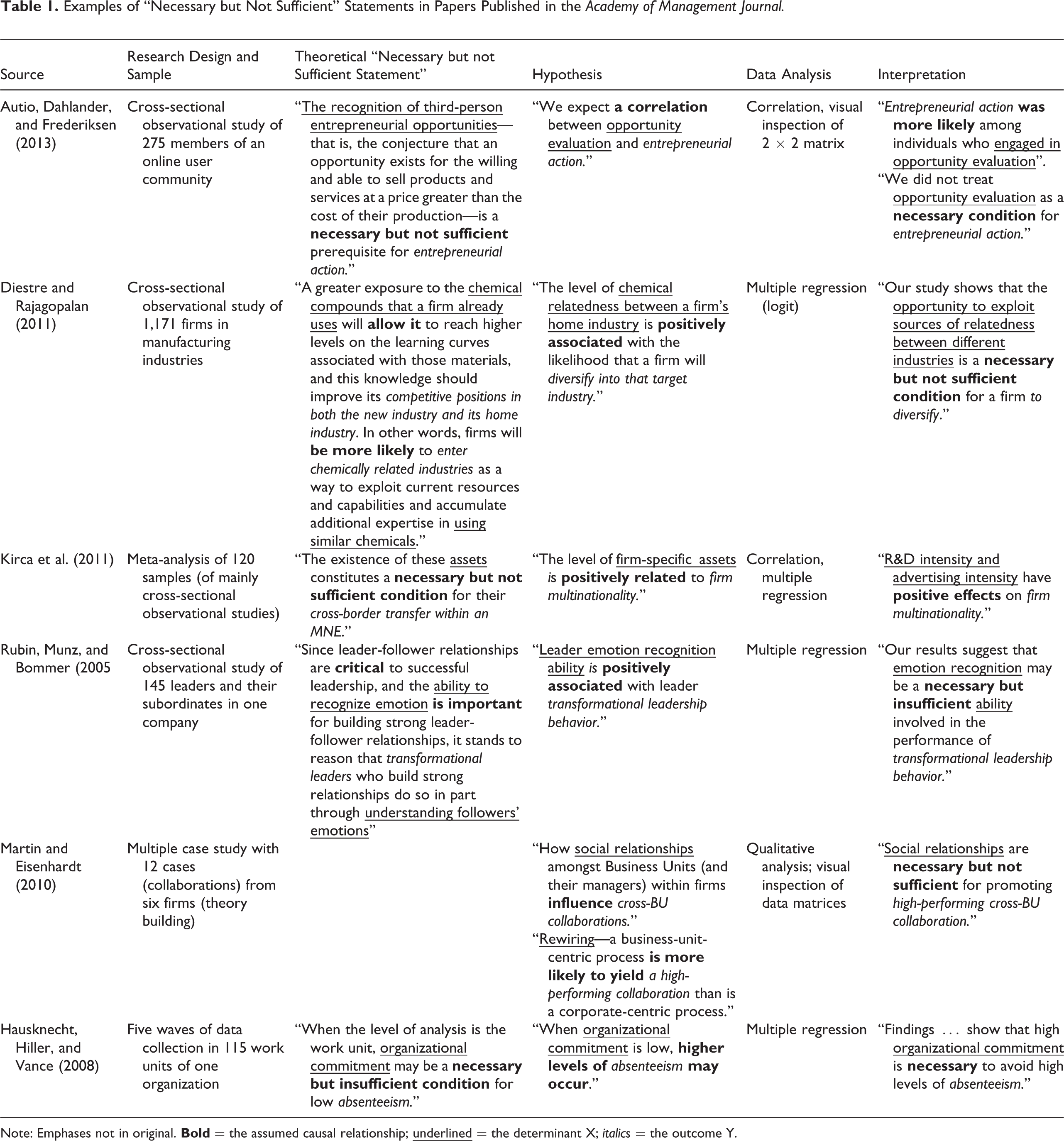
Note: Emphases not in original.
The table shows that researchers use traditional additive causality models and related data analysis approaches (e.g., correlation, regression) for empirically testing or inducing necessary but not sufficient statements. I would like to add one important caveat with respect to the papers included in Table 1. The authors of these papers are pursuing relevant research questions; unfortunately, the existing library of data analytic tools was not specifically developed to address these types of questions. Consequently, the authors were restricted to using traditional analytical tools. Thus, my criticism is not directed at the authors or how they approached their data analysis. My criticism is related to the lack of tools that were available to these authors. One of the goals of the current paper is to introduce a new set of analytical tools that may be of value to researchers pursuing questions such as those summarized in Table 1.
With that caveat in place, many of the papers presented in Table 1 (and identified during my review but not included in Table 1) tend to adhere to the following methodological sequence: A theoretical necessary but not sufficient statement is introduced in the Introduction, Theory, or Hypotheses section. This statement is reformulated as a traditional hypothesis with an unspecified “positive association” (or similar) between determinant and outcome (i.e., without specifying that the determinant is considered as necessary but not sufficient). The obtained observational data are analyzed using traditional variants of the general linear model (e.g., correlation or regression). If the hypothesis is supported (e.g., a positive association found between determinant and effect), the results are interpreted as a support of the necessary but not sufficient statement.
Consider a few illustrative examples from Table 1. Kirca et al. (2011) studied firm-specific assets as a cause of multinationality of international firms (which is a driver of performance of such firms) and stated in their Theory and Hypotheses section that R&D intensity and advertising intensity are firm-specific assets that “constitute a necessary but not sufficient [italics added] condition for their cross border transfer within an MNE” (p. 50). Subsequently, they reformulated this relationship as “the level of firm-specific assets is positively related [italics added] to firm multinationality” (p. 50) and tested and confirmed this hypothesis using traditional correlation and regression analyses. In another example, Rubin, Munz, and Bommer (2005) studied the effect on transformational leadership behavior of a leader’s ability to recognize a follower’s emotion and formulated the hypothesis that “leader emotion recognition ability is positively associated [italics added] with leader transformational leadership behavior” (p. 848). Using regression analysis, they found support for this hypothesis and concluded in the Discussion section that “our results suggest that emotion recognition may be a necessary but insufficient [italics added] ability involved in the performance of transformational leadership behavior” (p. 854). In yet another example, Hausknecht, Hiller, and Vance (2008) studied effects of organizational commitment on work unit absenteeism and claimed in their Theory and Hypotheses section that “organizational commitment may be a necessary but not sufficient condition for low absenteeism.” But then they reformulated the statement in sufficiency terms as “when organizational commitment is low, higher levels of absenteeism may occur [italics added]” (p. 1226), tested it by using traditional regression analysis, and claimed in the Discussion section that “findings … show that high organizational commitment is necessary [italics added] to avoid high levels of absenteeism” (p. 1239).
In each of the aforementioned examples, the authors were restricted in how they could go about testing or inducing a hypothesis framed in terms of necessary but not sufficient relationships. The aforementioned examples are simply illustrative and are not unique to this set of authors or this literature. Instead, they demonstrate how (across a wide range of management topics) researchers seek to test or induce necessary but not sufficient hypotheses but lack the proper analytical tools for doing so. Researchers are often unaware of the importance, special characteristics, and required methodology of the necessary but not sufficient approach. In this article, such an alternative data analysis approach is presented. Instead of drawing trend lines “through the middle of the data” in scatterplots (e.g., regression lines), it searches for empty areas in scatterplots and draws “ceiling lines” that separate empty and full data areas (for a detailed discussion on ceiling lines, see subsection Ceiling Techniques). I will distinguish between three types of necessary conditions, dichotomous, discrete, and continuous, and will use three illustrative examples to explain their similarities and differences: I will extend on the aforementioned dichotomous example of necessary GRE scores for admission (Vaisey, 2009), present a discrete example from Table 1 about necessary representation in a collaboration team for successful collaboration (Martin & Eisenhardt, 2010), and discuss a continuous example about necessary personality traits for sales performance (Hogan & Hogan, 2007). I integrate earlier work and ideas on analyzing dichotomous necessary conditions (e.g., Braumoeller & Goertz, 2000; Dul et al., 2010), discrete necessary conditions (e.g., Dul et al., 2010), and continuous necessary conditions (e.g., Goertz, 2003; Goertz, Hak, & Dul, 2013) and combine these with new ideas, for example, multivariate necessary condition, bottleneck technique, necessity inefficiency, effect size of a necessary condition, and techniques for drawing ceiling lines. I also present practical recommendations and software to guide researchers to perform an NCA analysis.
I consider NCA as a complement, not a replacement, of traditional approaches to analyze causal relations. NCA may provide new insights that are normally not discovered with traditional approaches: Multiple regression may spot determinants that (on average) contribute to the outcome (i.e., determinants with large regression coefficients), whereas NCA may spot necessary (critical) determinants that prevent an outcome to occur (constraints or bottlenecks). When bottlenecks are present, performance will not improve by increasing the values of other determinants (e.g., determinants with large regression coefficients) unless the bottleneck is taken away first (e.g., by increasing the value of the critical determinant). Only in those situations when none of the determinants are critical for reaching a desired outcome can traditional approaches inform us how to increase performance. Therefore, NCA may precede traditional approaches. This necessary but not sufficient approach is needed because critical determinants may or may not be part of lists of determinants identified with traditional approaches. Furthermore, due to the fundamental difference between the two approaches, determinants that show small or zero effects in traditional approaches may be identified as critical in the necessary but not sufficient approach (e.g., see the example presented in Figure 4), and determinants that show large effects in traditional approaches may not be critical according to the necessary but not sufficient approach. Indeed, both approaches are essential for a proper understanding of organizational phenomena. The NCA approach also adds to insights obtained from qualitative comparative analysis (QCA) (Ragin, 2000, 2008), which is another approach that understands causality in terms of necessity and sufficiency rather than correlation or regression. NCA focuses on (levels of) single determinants (and their combinations) that are necessary but not automatically sufficient, whereas QCA focuses on combinations of determinants (configurations) that are sufficient but not automatically necessary. Although QCA centers on sufficient configurations, it can also analyze single necessary conditions, but it does so in a limited way (for a further discussion on the difference between NCA and QCA see subsection Comparison NCA With QCA).
In what follows, I first discuss the logic of necessary conditions in more detail. Next, I present the NCA methodology by discussing ceiling techniques, effect size of the necessary condition, necessity inefficiency, the comparison of NCA with QCA, and limitations of NCA. Finally, I offer practical recommendations and free software for applying NCA.
The Logic of Necessary Conditions
In the aforementioned examples, both the condition (GRE score, fuel, trust) and the outcome (admission, moving car, solid financial system) can have only two values: absent or present. This is the dichotomous logic of necessary conditions, which is part of classic binary (or in mathematics, Boolean) logic. However, many real-life situations are not inherently dichotomous (although they can be dichotomized). In the discrete situation, the necessary condition and the outcome can have more than two values (e.g., low, medium, high), and in the continuous situation, any value is possible. In this section, I discuss the logic of necessary conditions by moving from the dichotomous, via the discrete, toward the continuous necessary condition.
Dichotomous Necessary Condition
Figure 1 (top) shows two ways to graphically represent the dichotomous necessary condition. On the left, possible observations for a necessary condition are plotted in the center of cells of a contingency matrix (I will use the convention that the X axis is “horizontal” and the Y axis is “vertical” and that values increase “upward” and “to the right” 4 ). The contingency matrix is a common way to present dichotomous necessary conditions (e.g., Braumoeller & Goertz, 2000; Dul et al., 2010). On the right, the possible observations are plotted on a grid of a Cartesian coordinate system. This representation is used here to facilitate the generalization of necessary condition characteristics from dichotomous logic toward discrete and continuous logic (described later in the article). The dashed lines are the ceiling lines that separate the area with observations from the area without observations.
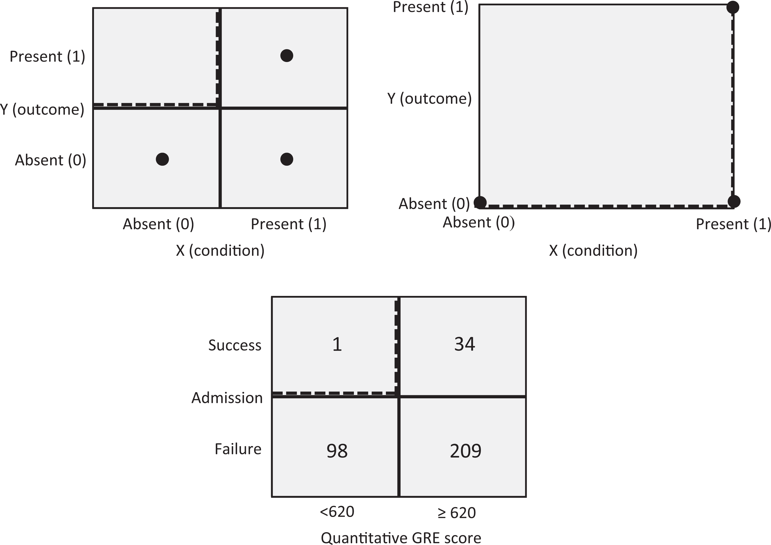
The dichotomous necessary condition with possible observations shown in the center of the cells of a contingency matrix (top left) and in the grid of a Cartesian coordinate system (top right).
The figure (top) shows that outcome Y = 1 is only possible if X = 1; however, if X = 1, two outcomes are possible, Y = 0 and Y = 1. Therefore X = 1 is necessary but not sufficient for Y = 1. However, if X = 0, then Y = 0, the absence of X is sufficient for the absence of Y. The necessity of the presence of X for the presence of Y and the sufficiency of the absence of X for the absence of Y are logically equivalent. Hume’s (1777) statement mentioned in the introduction section of this, namely, “if the first had not been, the second never had existed,” is the sufficiency of absence version of the necessary condition formulation.
The sufficiency of absence formulation of the necessary condition allows the value of X = 0 to be considered as a constraint or bottleneck for achieving the high value of the outcome (Y = 1). The empty cell for X = 0, Y = 1 indicates that a high value of Y = 1 cannot be achieved for the low value of X = 0. If the high Y value is to be achieved, the bottleneck must be removed by realizing a high value of X. On the other hand, the necessity of presence formulation of the necessary condition refers to the general organizational challenge of putting in place the right level of scarce resources or (managerial) effort to be able to reach a desired level of organizational performance (the outcome). Then X can be considered as an organizational ingredient (scarce event/characteristic/resource/effort) that is needed and therefore allows the desired organizational outcome Y (good performance) to occur.
The two versions of the same logic imply two possible ways of testing or inducing necessary conditions with data sets of observations (Dul et al., 2010). In the first way, different to traditional correlation or regression analyses, only successful cases are purposively sampled (for an everyday example, see Appendix A). Conversely, a correlation or regression analysis requires variance in the dependent variable, hence, then both successful and unsuccessful cases must be randomly sampled, and the analysis shows the extent to which determinants on average contribute to success. In NCA, the presence or absence of the condition is determined in cases with the outcome present (successful cases: Y = 1). The presence of the condition in successful cases is an indication of necessity of X = 1 for Y = 1. 5 If the condition is not present in the successful cases, then X is not necessary for Y. This approach was used by the current editor of Organizational Research Methods (ORM) before he took office as editor in July 2013. He performed a Google Scholar search to identify highly cited ORM papers and their common characteristics and found, for example, that such papers give practical recommendations to the organizational researcher (LeBreton, personal communication June 26, 2014). Additionally, in his first editorial, LeBreton (2014) states that “over the past 10 years, I have spent considerable time pondering what makes an impactful methods article. I have concluded that such articles share the following characteristics” (p. 114). The editor (implicitly) performed a necessary condition analysis: selecting cases purposively on the basis of the presence of the dependent variable (successful cases, i.e., highly cited papers) and identifying common determinants that were present in these cases. This resulted in necessary conditions for a highly cited paper in ORM, and several of these are listed in the editorial to stimulate authors, reviewers, and editors to produce impact papers in ORM by ensuring that the necessary conditions are in place (although this does not guarantee impact success). Necessary condition analysis is an effective and efficient way to find relevant variables that must be managed for success.
In the second approach to test necessary conditions, cases are selected in which the condition is absent (X = 0). The absence of the outcome in cases without the condition is an indication of necessity of X for Y. If success is present in cases without the condition, X is not necessary for Y. The editor could have searched for papers without practical recommendations to organizational researchers and—if the necessary condition holds—would have found that these papers are not highly cited. Normally, this second approach to test necessary conditions is much less efficient than the first one.
Two other approaches for selecting cases will not work. It is a common misunderstanding that necessary conditions can be detected by selecting and evaluating failure cases. There is no point in evaluating the characteristics of papers that are not highly cited. Figure 1 (top) shows that falsification of a necessary condition is not possible with failure cases (Y = 0) because the condition can be both absent (X = 0) and present (X = 1). In a similar way, an analysis of cases where the condition is present is not insightful either. A necessary condition is characterized by having no observations in the upper left corner. Therefore, the analysis of necessary but not sufficient conditions is about “the search for empty space” in the upper left corner. This applies not only to the dichotomous case but also to the discrete and continuous cases. 6
Illustrative Example of the Dichotomous Necessary Condition
Figure 1 (bottom) shows an example of Quantitative GRE scores of 342 students applying for admission to the Berkeley Sociology Graduate Program in 2009 (Goertz & Mahoney, 2012; Vaisey, 2009). A traditional data analysis to test the association between GRE score and admission would show a high correlation between the two variables (tetrachoric correlation coefficient = 0.6). The data justify the conclusion that success is more likely when the GRE score is at least 620 than when it is below 620. However, the necessary but not sufficient interpretation of the data is that a score of at least 620 is a virtual 7 (only one exception) necessary condition for admission. The exception is a student who was admitted based on a faculty member’s explicit testimony to the student’s quantitative abilities, which was regarded as superior information to the quantitative GRE score (Vaisey, personal communication, July 2, 2014). The upper left corner of Figure 1 is almost empty. Virtually all students (99%) who scored below 620 failed to be admitted. But scoring at least 620 did not guarantee success: Only 14% of these students succeeded in being admitted. Having a score below 620 is a bottleneck for being admitted. There may be other bottlenecks as well (e.g., a TOEFL score below 100). Advising students based on a traditional analysis would be to score high on GRE and TOEFL to increase your chances for success, whereas advising them based on a necessary but not sufficient analysis would add and make sure that you reach all minimum requirements to avoid guaranteed failure because you cannot compensate an inadequate score for one requirement with a high score for another one.
Discrete Necessary Condition
In the organizational sciences, variables are often scored by a limited number of discrete values, which usually have a meaningful order (ordinal scale), for example, a value can be higher/more/better than another value. Additionally, the differences between ordinal values can be meaningful, for example, the difference between high and medium may be the same as the difference between medium and low (interval scale). Many data in organizational sciences are obtained from measurements with respondents or informants using standardized questionnaires with Likert-type scales. In such an approach, a variable is usually represented by a group of items with several response categories. If interval properties are assumed, item responses can be combined (e.g., by adding or averaging) to obtain a score for the variable of interest. If items are scored on a discrete scale, the resulting score will be discrete as well. For example, if a variable is constructed from five items, each having seven response categories from 1 to 7, the number of discrete values of the variable is 31. 8
Figure 2 shows a trichotomous example of possible observations for a discrete necessary condition, where both X and Y have three possible values: low (0), medium (1), and high (2). The empty area in the upper left corner indicates the presence of a necessary condition. In this article, it is assumed that the ceiling line in a contingency table that separates the “empty” cells without observations from the “full” cells with observations as well as the ceiling line in a Cartesian coordinate system through the points on the border between the empty and the full zone are piecewise linear functions that do not decrease. 9 The question then is: “Which minimum level of the determinant X is necessary for which level of outcome Y”? Figure 2 (top) shows that for an outcome (performance) of Y = 2, it is necessary that the determinant (resource/effort) has value X = 2. However, X = 2 does not guarantee Y = 2. Therefore, X = 2 is necessary but not sufficient for Y = 2. For an outcome of Y = 1, it is necessary that the determinant has value of at least X = 1. However, X ≥ 1 does not guarantee Y = 1. Therefore, X ≥ 1 is necessary but not sufficient for Y = 1.
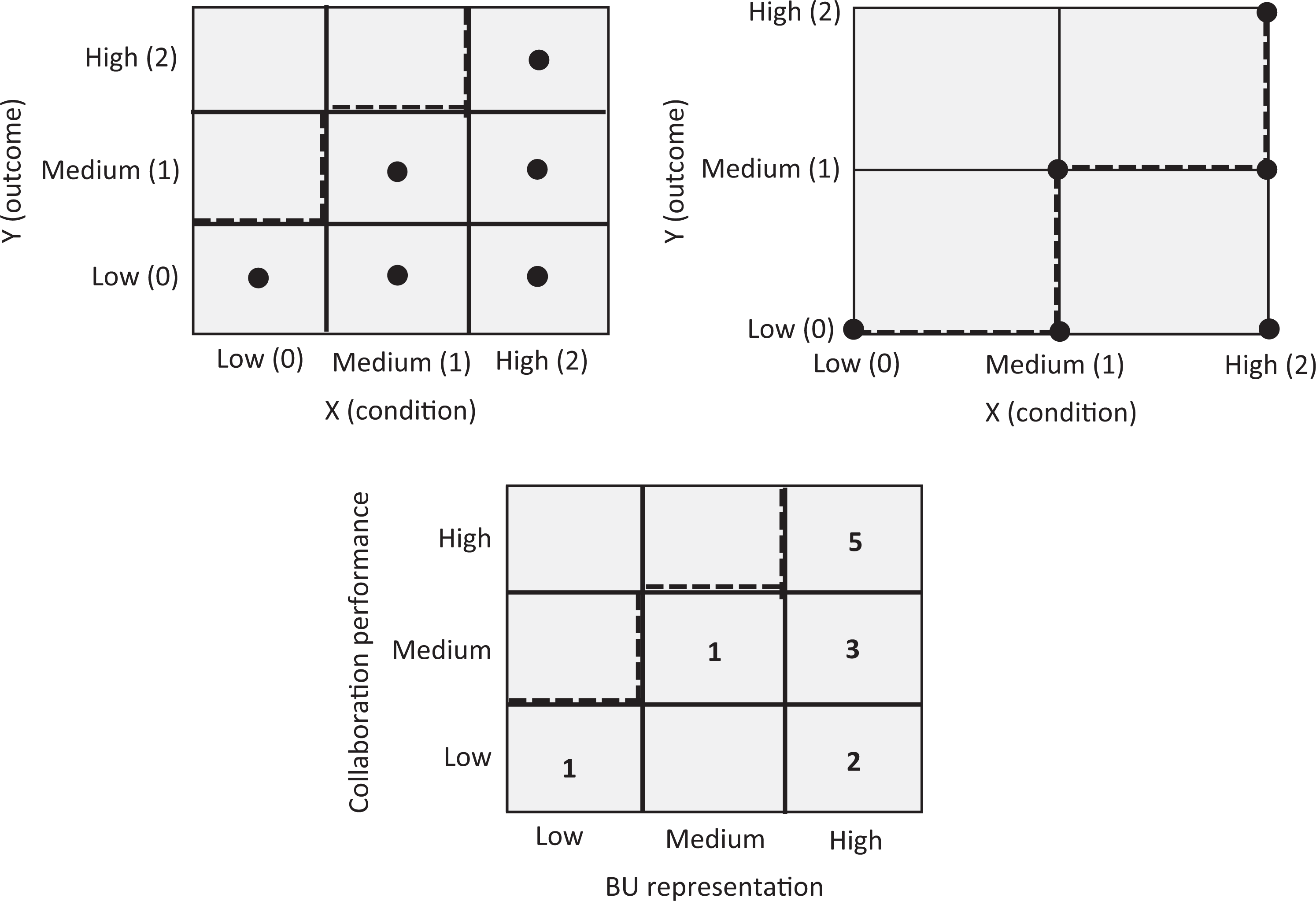
The discrete necessary condition with three levels, low (0), medium (1), high (2), in a contingency matrix (top left) and in the grid of a Cartesian coordinate system (top right).
Figure 2 (top) shows that the value X = 0 is a constraint for reaching both Y = 1 and Y = 2. The value X = 1 is a constraint for reaching only Y = 2. If the middle medium/medium cell (top left) or point (top right) were absent, the constraint of X = 1 would be stronger because X = 1 would then also constrain Y = 1. The size of the empty zone is an indication of the strength of the constraint of X on Y (more details follow in subsection Effect Size of the Necessary Condition). Also, for testing or finding discrete necessary conditions, cases can be selected purposively on the bases of the presence of the dependent variable. If one is interested in necessary conditions for Y = 2, then cases where this outcome is present (successful cases: Y = 2) are selected and the level of the condition X is observed. If in all successful cases no X is smaller than X = 2, X = 2 can be considered as necessary for Y = 2. Similarly, if one is interested in necessary conditions for Y = 1, then cases with this outcome are selected. If in all these cases no X is smaller than X = 1 (i.e., X ≥ 1), then it can be considered that X ≥ 1 is necessary for Y = 1. The aforementioned analyses of discrete necessary conditions can be applied to both ordinal variables (with Figure 2, top left) and interval variables (with Figure 2, top left or right; the Cartesian coordinate system assumes known order and distances between the category values) and can be extended with more discrete categories. A discrete necessary condition with a large number of categories nears a continuous necessary condition.
Illustrative Example of the Discrete Necessary Condition
In a multiple case study, Martin and Eisenhardt (2010) analyzed success of collaboration between business units in multi-business firms. From their data, a discrete (trichotomous) necessary condition on the relationship between “business unit [BU] representation” in the collaboration team and “collaboration performance” can be derived (see Appendix B), which is shown in Figure 2 (bottom). It turns out that a “high” level of BU representation is necessary but not sufficient for a “high” level of collaboration performance. All five highly successful cases (collaborations) have this high level of BU representation. There are also five other cases with “high” level BU representation, but these cases apparently did not achieve the highest level of performance. If only a “medium” level of collaboration performance were desired, then at least a “medium” level of BU representation is necessary, but again this is not sufficient because two collaborations had higher than medium levels of BU representation and showed “low” performance. This analysis results in two necessary (but not sufficient) propositions: “A high level of BU representation is necessary but not sufficient for a high-performing cross-business unit collaboration” and “At least a medium level of BU representation is necessary but not sufficient for a medium level of cross-business unit collaboration performance.” These propositions are different and more specific than the corresponding traditional proposition proposed by Martin and Eisenhardt (2010), which are implicitly formulated in terms of sufficiency: “BU representation is more likely to yield high collaboration performance.” Other examples of necessary condition hypotheses derived from Martin and Eisenhardt’s (2010) data set are presented in Appendix B.
In comparison to the dichotomous necessary condition analysis, the discrete necessary condition adds more variable levels to the analysis and can therefore provide more specific propositions. The trichotomous necessary condition in Figure 2 shows which levels of the determinant (medium or high) are necessary for reaching the desired level of collaboration performance (medium or high). Sometimes a medium level of the determinant may be enough for allowing the highest level of performance. Then, a higher level of the determinant may be “inefficient” (a further discussion on necessity inefficiency is presented in subsection Necessity Inefficiency).
Continuous Necessary Condition
In the case of a continuous necessary condition, the determinant X and the outcome Y are continuous variables (ratio variables). This means that the condition and the outcome can have any value within the limits of the lowest (0%) and highest (100%) values, allowing for even further detail. 10 Figure 3 contains graphs that correspond to the continuous necessary condition. The empty zone without observations is separated from the zone with observations by a straight ceiling line. In general, a ceiling is a boundary that splits a space in an upper part and a lower part, with only feasible points in the lower part of the space. In the two-dimensional Euclidian space (XY-plane), the expression X is necessary but not sufficient for Y is graphically represented by the ceiling line Y = f(X), with inequality Y ≤ f(X) representing the feasible points in the lower part of the space (on and below the ceiling line). For the linear two-dimensional case, the ceiling line is a straight line Y = aX + b (a = slope; b = intercept) with Y ≤ aX + b representing the lower part with the feasible XY-points. In this article, it is assumed that the ceiling line is linear and does not decrease. 11
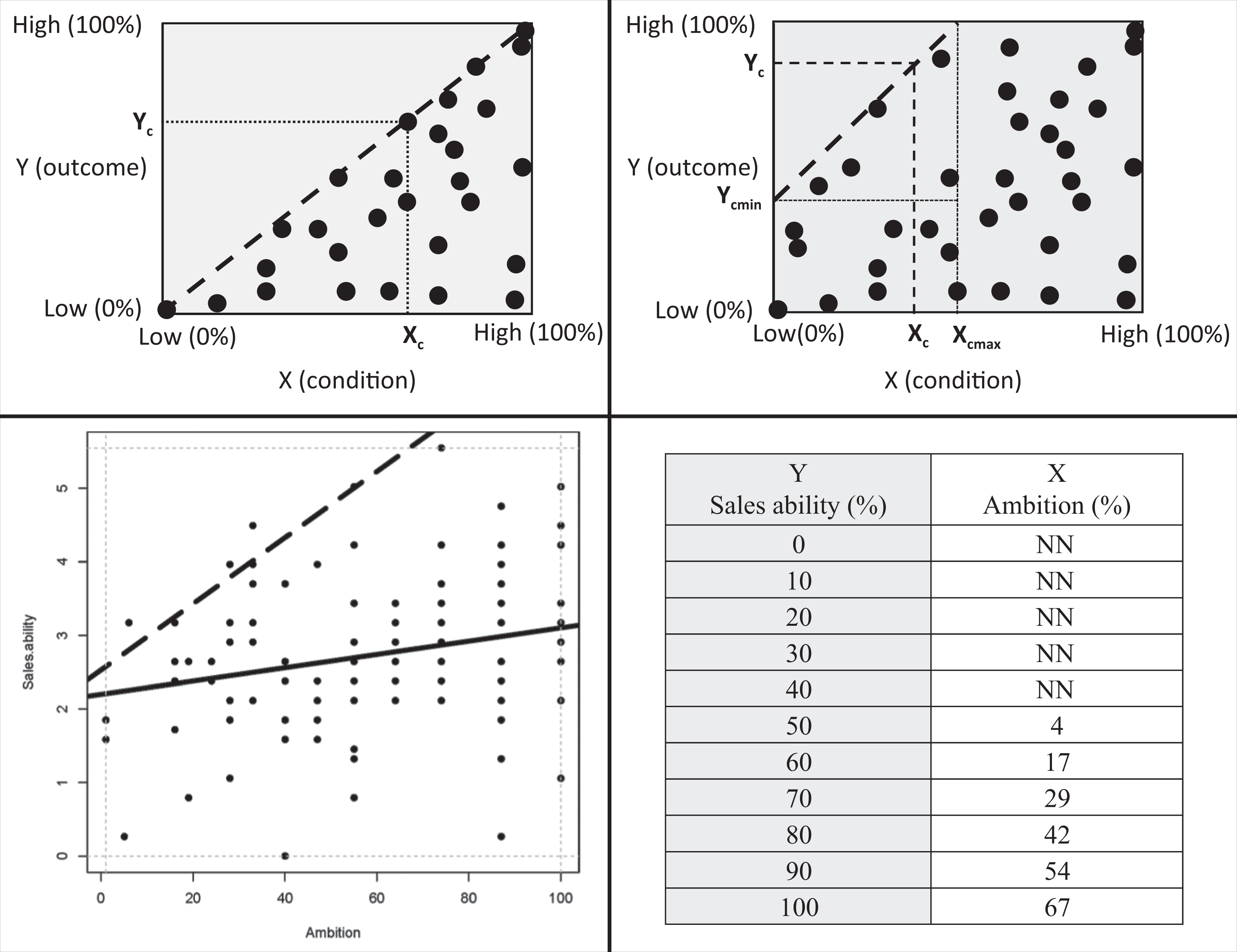
The continuous necessary condition with a large number of X and Y levels between low (0%) and high (100%), plotted in a Cartesian coordinate system. Note: The dashed line is the ceiling line. Top left: Idealized (“triangular”) scatterplot; the ceiling line coincides with the diagonal. Top right: Common (“pentagonal”) scatterplot; the ceiling line intersects X = XLow and Y = YHigh axes at other points than (XLow, YLow) and (XHigh, YHigh). The upper left area between the lines X = Xcmax and Y = Ycmin is the necessary condition zone where each X constrains Y and each Y is constrained by X. Bottom left: Example of a continuous necessary but not sufficient condition: Employee ambition is necessary but not sufficient for sales ability. The selected ceiling line technique (ceiling regression with free disposal hull) allows some data points above the ceiling line (see subsection Ceiling Techniques). The solid line through the middle of the data is the ordinary least squares regression line. Bottom right: Bottleneck table for the example illustrating what minimum level of the necessary conditions (X = Ambition) is required for different desired levels of the outcome (Y = Sales Ability). NN = not necessary. Source: Data obtained from Jeffrey Foster, Vice President of Science, Hogan Assessments, July 9-11, 2014.
The continuous necessary condition logic implies that a certain desired level of the outcome (Y = Yc) can only be achieved if X ≥ Xc. This means that Xc is necessary for Yc, but Xc is not sufficient for Yc because there may be observations X = Xc with Y < Yc, hence there are observations below the ceiling line for a given Xc. Within the scope of possible XY-values, the feasible necessary but not sufficient space in Figure 3 (top left) is the triangular space below the ceiling line: The ceiling line coincides with the diagonal of the scope. Although it is frequently stated that the necessary but not sufficient condition can be graphically represented by a triangular shape of the feasible area (Goertz & Starr, 2003; Ragin, 2000), this shape is just a special case of the more common pentagonal shape (Figure 3, top right). In the present article, we focus on the general linear ceiling line with a typical pentagonal feasible space. In traditional approaches, heteroskedasticity in such scatter plots (increasing variance with increasing X) is considered a concern for performing standard regression analysis, whereas it is inherent to the necessary but not sufficient logic. Traditional approaches draw average lines through the middle of the data (average trends), whereas NCA draws borderlines between the zone with and the zone without observations in the left upper corner. Therefore, traditional approaches to analyze pentagonal scatterplots may disconfirm X causes Y because the regression line may be virtually horizontal, but the NCA approach may confirm X causes Y because there is an empty zone in the upper left corner.
The presence and size of an empty zone is an indication of the presence of a necessary condition. The empty zone in the upper left corner reflects the constraint that X puts on Y. For example, the value X = Xc is a constraint (bottleneck) for reaching level of Y > Yc. A higher level of Y is only possible by increasing X. Also, for testing or inducing continuous necessary conditions, cases can be selected purposively on the bases of the presence of the dependent variable. If one is interested in necessary conditions for Y > Y*, then cases where this outcome is present (successful cases: Y > Y*) are selected, the cases are plotted in a Cartesian coordinate system, and a ceiling line is drawn to represent the necessary condition Xc for Yc (see the subsection Ceiling Techniques).
Illustrative Example of the Continuous Necessary Condition
The Hogan Personality Inventory (HPI) is a widely used tool to assess employee personality for predicting organizational performance (Hogan & Hogan, 2007). Figure 3 (bottom left) shows an example of the relationship between the HPI ambition score (one’s level of drive and achievement orientation) and supervisor rating of sales ability in a data set of 108 sales representatives from a large food manufacturer in the United States. Employees completed the HPI and supervisors rated employee’s performance in term of sales ability using a seven-item reflective scale (e.g., “seeks out and develops new clients”).
A traditional data analysis of the relationship between ambition and sales ability would consist of an ordinary least squares (OLS) regression line through the middle of the data (solid line in Figure 3, bottom left). This line runs slightly upwards, indicating a small positive average effect of ambition on sales ability (R 2 = 0.07). The data justify the conclusion that on average more ambition results in more sales ability, but this is possibly not practically relevant because of the small effect size. However, the necessary but not sufficient interpretation of the data is that the empty zone in the upper left corner indicates that there is a necessary condition. The ceiling line indicates that there is a ceiling on sales ability depending on the sales representative’s level of ambition. The CR-FDH technique (fully explained in the Ceiling Techniques subsection) that is used in this example to draw ceiling lines allows some data points above the ceiling line. For a desired sales ability Level 4, it is necessary to have an ambition level of at least 30. About 20% of the sales representatives in the sample do not reach this level of ambition, which suggests that people with ambition levels below 30 will certainly fail to reach a sales ability level of 4 of higher. The other, about 80%, sales representatives who do have an ambition level of at least 30 could reach such a high level of sales ability, but this is not guaranteed; in fact, only about 10% of the sales representatives in the sample obtained this level of sales ability. In other words, an ambition level of at least 30 is necessary but not sufficient for a sales ability level of at least 4. An ambition level below 30 is a bottleneck for this high level of sales ability. Figure 3 (bottom right) shows the bottleneck technique, which is a table that indicates which level of the necessary condition (Ambition) is necessary for a given desired level of outcome (Sales Ability in %), according to the ceiling line.
Multivariate Necessary Condition
Until now, the analysis was bivariate with one X that is necessary for one Y. In this subsection, a more complex situation is considered: more than one necessary condition (X1, X2, X3, etc.) and one Y. Multicausality is common in the organizational sciences. For example, Finney and Corbett (2007) reviewed empirical research on Enterprise Resource Planning (ERP) implementation success and identified 26 organizational determinants of success. Evanschitzky, Eisend, Calantone, and Jiang (2012) performed a meta-analysis of empirical research and identified 20 determinants of product innovation success. These examples can be extended with many other examples from virtually any subfield in the organizational sciences: A large set of determinants contribute to the outcome, and the underlying studies utilize traditional approaches such as correlation and regression to identify these determinants. Then, the size of the correlation or regression coefficient indicates the importance of a determinant. In this traditional logic, several determinants (X1, X2, X3 … ) contribute to the outcome and can compensate for each other. In necessary but not sufficient logic, each single necessary determinant Xi always needs to have its minimum level Xic to allow Yc, independent of the value of the other determinants. If Xi drops below Xic, the other determinants cannot compensate it. After the drop, the desired outcome Yc can only be achieved again if Xi increases toward Xic. This absence of a compensation mechanism once again shows the practical importance of identifying necessary conditions: putting minimum required levels of it in place and keeping these levels in place: “Satisfying necessary conditions … constitutes the foundation of achieving the goal” (Dettmer, 1998, p. 6).
Illustrative Example of the Multivariate Necessary Condition
As an example, the upper part of Figure 4 shows the scatterplots of four personality scores measured with the Hogan Personality Inventory (HPI) in the same sample as presented earlier. The plot for the first HPI score Ambition is the same as Figure 3 (bottom left). The other three scatterplots are for HPI scores Sociability, Interpersonal Sensitivity, and Learning Approach. The regression lines (solid lines through the middle) show that all four personality traits have a relatively small effect on Sales Ability. Ambition and Sociability have a small positive effect. The Interpersonal Sensitivity regression line is nearly horizontal. The Learning Approach regression line is slightly negative (!), indicating that on average Learning Approach has a small negative effect on Sales Ability. A traditional multiple regression analysis indicates that the four personality traits together hardly predict performance (adjusted R 2 = 0.10). Yet, all four plots, including the plot for Learning Approach, show an empty space in the upper left corner, indicating that each personality trait may be necessary but not sufficient for Sales Ability. The necessary condition analysis predicts failure in these zones: The level of Y cannot be reached with the corresponding level of X. This applies to each determinant separately.
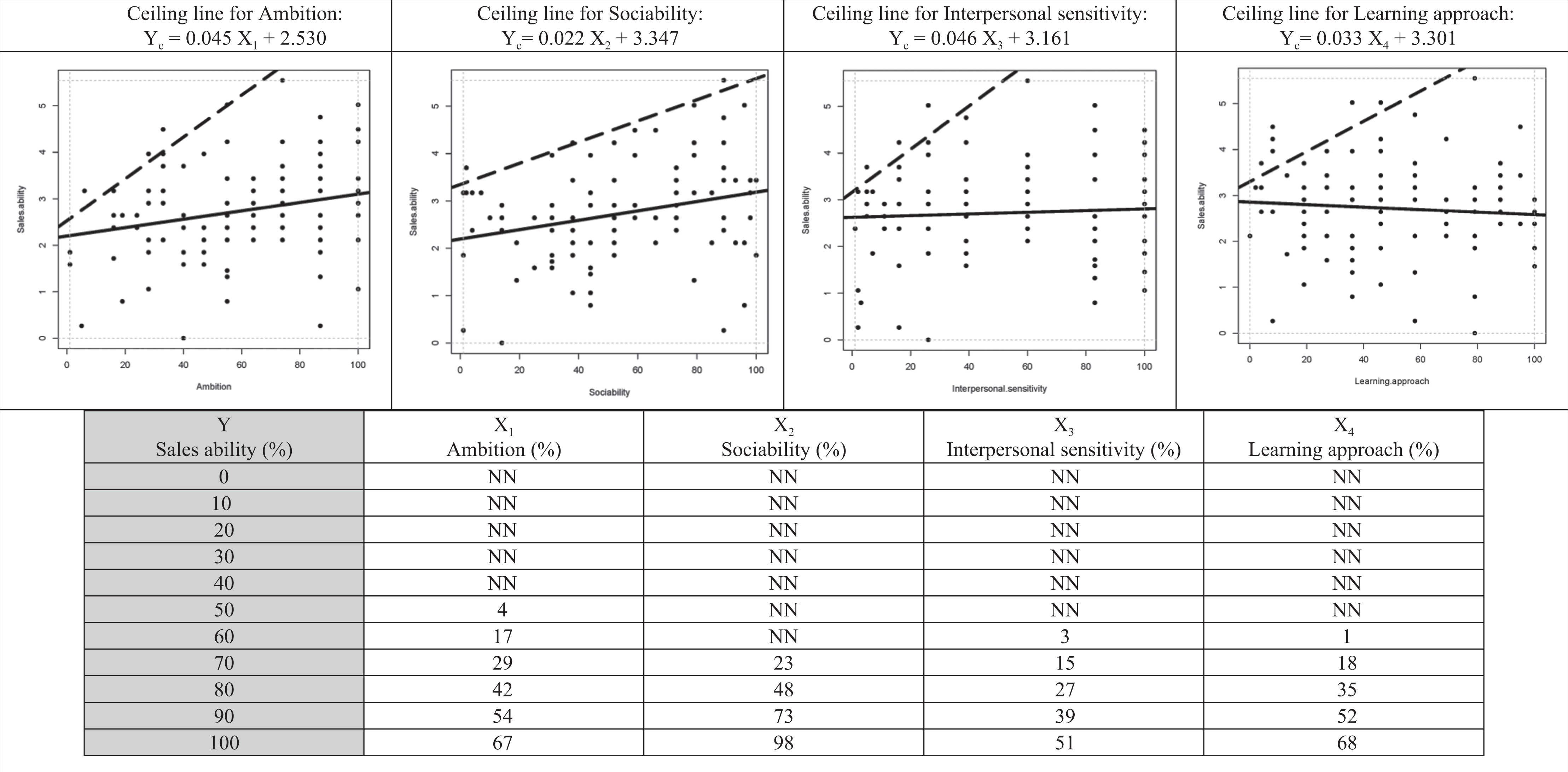
Example (see note 25) of the multivariate necessary condition with four necessary conditions. Note: The dashed lines are ceiling lines. The selected ceiling line technique (ceiling regression with free disposal hull) allows some data points above the ceiling line (see subsection Ceiling Techniques). The solid line is the ordinary least squares regression line. Upper part: Ceiling lines for four necessary conditions (Ambition, Sociability, Interpersonal Sensitivity, Learning Approach). Lower part: Bottleneck table: required minimum levels of the necessary condition for different desired levels of the outcome (Sales Ability). NN = not necessary.
The empty zones have different shapes because the ceiling lines (dashed lines drawn by using the CR-FDH ceiling technique, see Ceiling Techniques subsection) have different intercepts and slopes (see the ceiling equations in Figure 4, top). It implies that the necessary determinants put different constraints on the outcome. 12 This is illustrated with the multivariate bottleneck technique. The bottleneck table in the lower part of Figure 4 shows that for a desired level of outcome Yc = 80 (80% of the range of observed values; 0% = lowest, 100% = highest), the necessary levels of X1, X2, X3, and X4 are different: X1c = 42, X2c = 48, X3c = 27, and X4c = 35. A few important points are worth noting. First, we should recognize that each X variable must obtain these minimum ceiling values (Xi ≥ Xic) before it is possible to obtain Yc = 80. Thus, if even one of the Xi values falls below its ceiling value, Yc = 80 will not be reached. This contrasts with traditional applications of the general linear model, where the X variables are allowed to operate in a compensatory manner (e.g., a low score on X1 may be compensated for with a higher score on X2). Second, it is also important to recognize that the ceiling values will change if we change the level of the desired outcome. For Yc = 100, X1c = 67, X2c = 98, X3c = 51, and X3c = 68. Finally, it is also possible that for a given (lower) desired value of the outcome, one or more determinants are no longer necessary. For example, for Yc = 60 or lower, determinant X2 (Sociability) is no longer a bottleneck. For Yc = 50 or lower, also X3 (Interpersonal Sensitivity) and X4 (Learning Approach) are no longer a bottleneck, and none of the determinants are necessary for Yc ≤ 40.
It is typical for multivariate necessary conditions that no determinant is necessary at relatively low levels of the desired outcome, whereas several determinants become necessary at higher levels of desired outcome. Which specific determinant is the bottleneck depends on the specific levels of the determinants and the desired outcome. For example, if each of the four determinants has a score of 20, such an Ambition score and Sociability score allow a Sales Ability of at least 60, whereas such an Interpersonal Sensitivity score and Learning Approach score allow a Sales Ability of at least 70. Hence, a desired Sales Ability of 60 is possible with scores of 20 of the four HPI determinants, but a desired Sales Ability of 70 is not possible with such scores: The Ambition and Sociability scores are bottlenecks for such an outcome. The outcome of 70 is only possible if the Ambition score increases from 20 to at least 29 and the Sociability score from 20 to at least 23. The bottleneck table also shows that for a desired Sales Ability score below 40, no HPI score is a bottleneck, which illustrates “outcome inefficiency” and indicates that the outcome could be higher, even with low HPI scores (for a discussion on outcome inefficiency see subsection Necessity Inefficiency). The table also shows that for the highest outcome level (Sales Ability = 100), condition inefficiency is present: All HPI scores are smaller than100, with only the Sociability score close to 100. This indicates that for reaching the highest level of outcome, only about half to two-thirds of the maximum HPI scores for Ambition, Interpersonal Sensitivity, and Learning Approach are necessary, whereas for Sociability, the maximum HPI score is necessary (for a discussion on condition inefficiency see subsection Necessity Inefficiency).
Multivariate necessary condition analysis with the bottleneck technique identifies which determinants, from a set of necessary determinants, successively become the weakest links (bottlenecks, constraints) if the desired outcome increases. In other words, for a given level of the desired outcome, multivariate necessary condition analysis identifies the necessary (but not sufficient) minimum values of the determinants to make the desired outcome possible.
Necessary Condition Analysis
The continuous necessary condition case can be considered as the general case that includes the dichotomous and discrete cases (the graphs on the right sides in Figures 1 and 2 are essentially the same as the graphs in Figure 3). Therefore, the general methodology necessary condition analysis is developed for determining necessary (but not sufficient) conditions. This methodology consists of two main parts: (1) determining ceiling lines and the corresponding bottleneck tables and (2) calculating several parameters such as accuracy of the ceiling line, effect size of the necessary condition, and necessity inefficiency. First, I propose and evaluate two classes of ceiling techniques for drawing ceiling lines (ceiling envelopment and ceiling regression), compare these techniques and some other techniques, and present an example. Next, I develop an effect size measure for necessary conditions and propose benchmark values, discuss necessity inefficiency, and compare NCA with QCA. Finally, I discuss the limitations of NCA.
Ceiling Techniques
The starting point for the necessary condition analysis is a scatter plot of data using a Cartesian coordinate system, which plots X (the determinant and potential necessary condition) against Y (the outcome) for each case. If visual inspection suggests the presence of an empty zone in the upper left corner (with the convention that the X axis is “horizontal” and the Y axis is “vertical” and that values increase “upward” and “to the right”), a necessary condition of X for Y may exist. Then a ceiling line between the empty zone without observations and the full zone with observations can be drawn. A ceiling line must separate the empty zone from the full zone as accurately as possible. Accuracy means that the empty zone is as large as possible without observations in it. However, drawing the best ceiling line usually requires making a trade-off decision between the size of the empty zone and the number of observations in the empty zone (“exceptions,” “outliers,” “counterexamples”). Because the “empty” zone may not always be empty, it is named “ceiling zone” (C). The position of the data points around the ceiling line might suggest that the best ceiling line is not linear or increasing. Additionally, the best ceiling line may be a smooth line or a piecewise (linear) function. A ceiling function can be expressed in general terms as Yc = f (Xc). For simplicity, the focus in this article is on continuous or piecewise linear, nondecreasing ceiling lines, which appears acceptable for first estimations of ceiling lines for most data sets. A nondecreasing (constant or increasing) ceiling line is typical and allows for a formulation that X ≥ Xc is necessary for Yc.
Goertz et al. (2013) made the first attempts at drawing ceiling lines. They visually inspected the ceiling zone of a specific scatterplot and divided it manually into several rectangular zones. Rather than defining the ceiling line, the combination of rectangles resulted in a piecewise linear ceiling function with all observations on or below the ceiling. The advantage of this technique is that it implicitly only uses the location of upper left observations (where the border exists) to draw the ceiling line and that it can be made accurate with all observations on or below the ceiling line. One disadvantage of this technique is that it is informal and based on subjective selection of rectangles. Additionally, Goertz et al. introduced quantile regression to systematically draw continuous linear ceiling lines. Quantile regression (Koenker, 2005) uses all observations to draw lines. The 50th quantile regression line splits the observation in about half above and half below the line. This line is similar to a regular OLS regression line. However, for quantiles above, for example, 90, quantile regression results in a ceiling line that allows some points above the line. The advantage of this technique is that it is an objective, formal methodology to draw ceiling lines. However, a disadvantage is that it uses all observations below the ceiling line. For drawing a line between zones with and without observations, it may not be appropriate to use observations far away from this line.
For NCA, the advantages of the two approaches are combined by proposing two alternative classes of techniques, ceiling envelopment (CE) and ceiling regression (CR). Both are formal techniques and use only observations close to the ceiling zone. CE is a piecewise linear line and CR a continuous linear line (straight line).
Ceiling envelopment
In this article, ceiling envelopment is created for NCA on the basis of data envelopment analysis (DEA) techniques (Charnes, Cooper, & Rhodes, 1978). DEA is used in operations research and econometrics to evaluate production efficiency of decision-making units. Here the method is used to draw ceiling lines. Ceiling envelopment pulls an envelope along upper left observations using linear programming. Only a few assumptions need to be made regarding the shape of the ceiling line, depending on the specific envelopment technique. The ceiling envelopment technique with varying return to scale (CE-VRS) assumes that the ceiling line is convex. It results in a piecewise linear convex ceiling line. The envelopment technique with free disposal hull (CE-FDH) is a more flexible technique (Tulkens, 1993). It does not require many assumptions regarding the ceiling line. Because of its flexibility and intuitive and simple applicability to dichotomous, discrete, and continuous necessary conditions, CE-FDH is proposed as a default ceiling envelopment technique for NCA. It results in a piecewise linear function along the upper left observations. Drawing the CE-FDH ceiling line can be formulated in words as follows: Start at point Y = Ymin for observation X = Xmin. Move vertically upward to the observation with the largest Y for X = Xmin (there can be more than one observation with the same X value, particularly for discrete variables). Move horizontally to the right until the point with an observation on or above this horizontal line (discard observations below this line). Move vertically upward to the observation with the largest Y for this X (there can be more than one observations with the same X value, particularly for discrete variables). Repeat 3 and 4 until the horizontal line in 3 has reached the X = Xmax line.
Ceiling regression
In this article, ceiling regression is created for NCA on the basis of the outcomes of a CE analysis. Therefore, two versions exist: one based on the outcomes of CE-VRS and one based on the outcomes of CE-FDH. Ceiling regression CR-VRS draws an OLS regression line through the points that connect the linear pieces of the CE-VRS ceiling line, whereas CR-FDH draws an OLS regression line through the upper-left edges of the CE-FDH piecewise linear function, namely, the points where a vertical part of the CE-FDH line ends and continues as a horizontal line when X increases. These approaches smoothen the piecewise linear ceiling lines from the ceiling envelopment techniques by using a straight line. The straight line allows for further modeling and analyses and for comparison of ceiling lines. For the same reasons that CE-FDH is preferred over CE-VRS, CR-FDH is preferred over CR-VRS.
Comparison of ceiling techniques
Table 2 compares the four different ceiling techniques. It also includes some other common techniques in operations research and econometrics for the estimation of efficiency frontiers that could be used for drawing ceiling lines as well. Corrected ordinary least squares (COLS) and stochastic frontier analysis (SFA) (e.g., Aigner & Chu, 1968; Bogetoft & Otto, 2011) have some disadvantages compared to the techniques selected previously. COLS shifts the OLS regression line toward the most upper point and therefore uses all observations. SFA focuses on the observations around the ceiling line but includes a stochastic term based on a probability assumption of the observations below the ceiling and thus also uses all observations. A last technique called low-high (LH) was created for the purpose of NCA as a rough first estimation of the ceiling line. It is the diagonal of the necessary condition zone defined by two specific observations in the data set: the observation with the lowest X (with highest Y) and the observation with the highest Y (with lowest X). However, this technique is sensitive to outliers and measurement error.
Comparison of Techniques for Drawing Ceilings Lines.
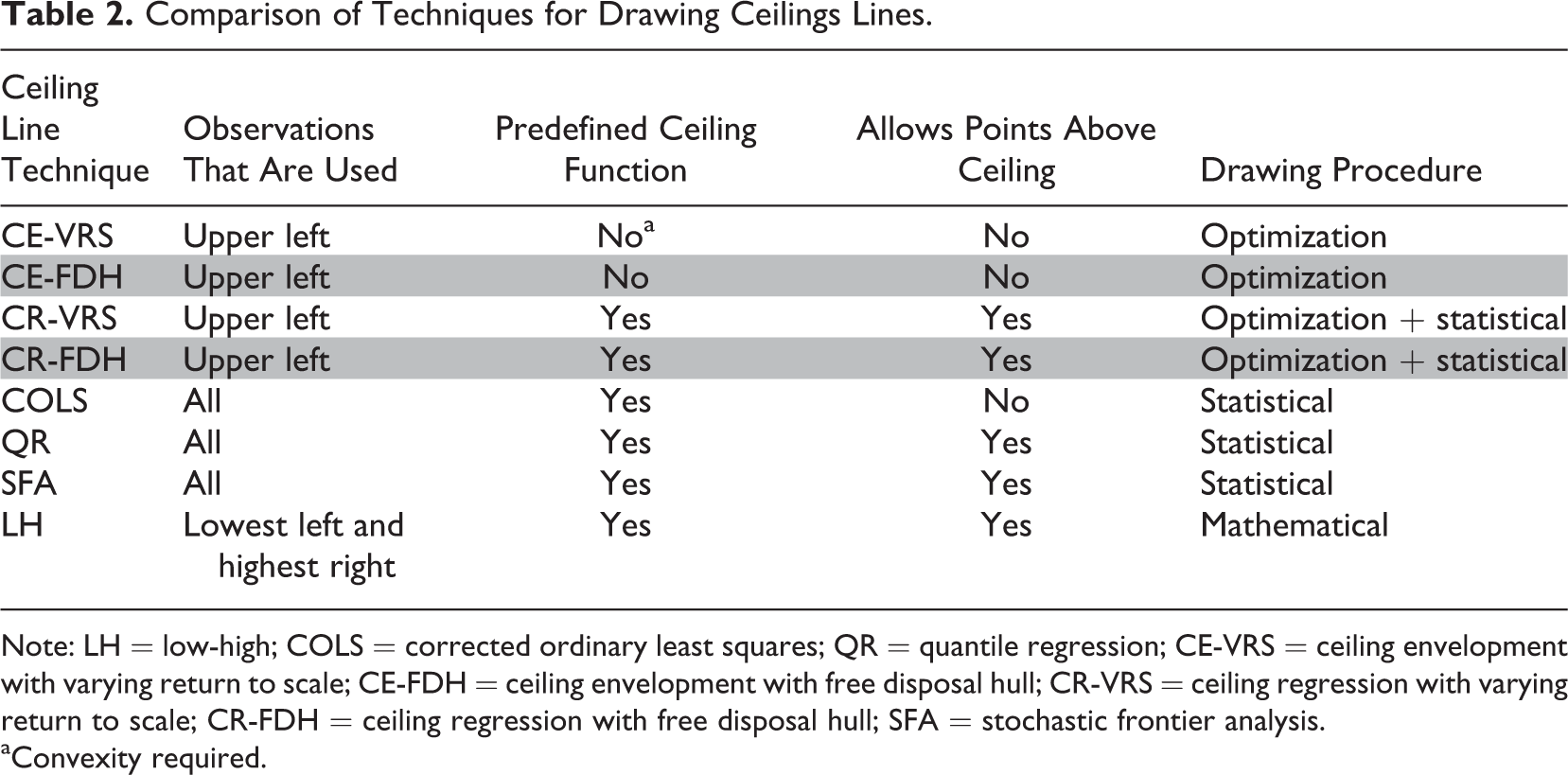
Note: LH = low-high; COLS = corrected ordinary least squares; QR = quantile regression; CE-VRS = ceiling envelopment with varying return to scale; CE-FDH = ceiling envelopment with free disposal hull; CR-VRS = ceiling regression with varying return to scale; CR-FDH = ceiling regression with free disposal hull; SFA = stochastic frontier analysis.
aConvexity required.
The table shows that only five techniques use upper left points (LH, CE-VRS, CE-FDH, CR-VRS, and CR-FDH) to draw the border line between zones with and zones without observations. Within this group, LH uses only two observations, whereas CE-VRS, CE-FDH, CR-VRS, and CR-FDH use observations close to the border line. When comparing CE-VRS and CE-FDH, the latter has fewer limitations because it does not require convexity of the ceiling function and is therefore preferred. Because CR-VRS and CR-FDH are based on CE-VRS and CE-FDH, respectively, CR-FDH also has fewer limitations. Therefore, CE-FDH is the default as a nonparametric technique (no assumption about ceiling line function), and CR-FDH is the default for a parametric technique (linear ceiling line). When comparing CE-FDH and CR-FDH, the former is preferred when a straight ceiling line does not properly represent the data along the border between the empty and full zone and when smoothing considerably reduces the size of the ceiling zone. This holds particularly for dichotomous variables and for discrete variables with a small number of variable levels (e.g., max 5; see Figure 2). This may also happen if the number of observations is relatively low, namely, in small data sets. If a straight ceiling line is an acceptable approximation of the data along the border, the CR-FDH technique is preferred. Compared to CE-FDH, CR-FDH usually has some observations in the ceiling zone due to the smoothing approach, and the ceiling zone may be somewhat smaller. By definition, CE-FDH does not have observations above the ceiling line; it is therefore more sensitive to outliers and measurement errors than CR-FDH.
Accuracy
The accuracy of a ceiling line is defined as the number of observations that are on or below the ceiling line divided by the total number of observations, multiplied by 100%. Then, by definition, the accuracy for CE-VRS, CE-FDH, and COLS is 100%, and for the other techniques, the accuracy can be below 100%.
Example
In Figure 5, the eight techniques are applied to a data set of 28 countries with data about a country’s level of individualism according to Hofstede (1980) and a country’s innovation performance according to the Global Innovation Index (Gans & Stern, 2003).
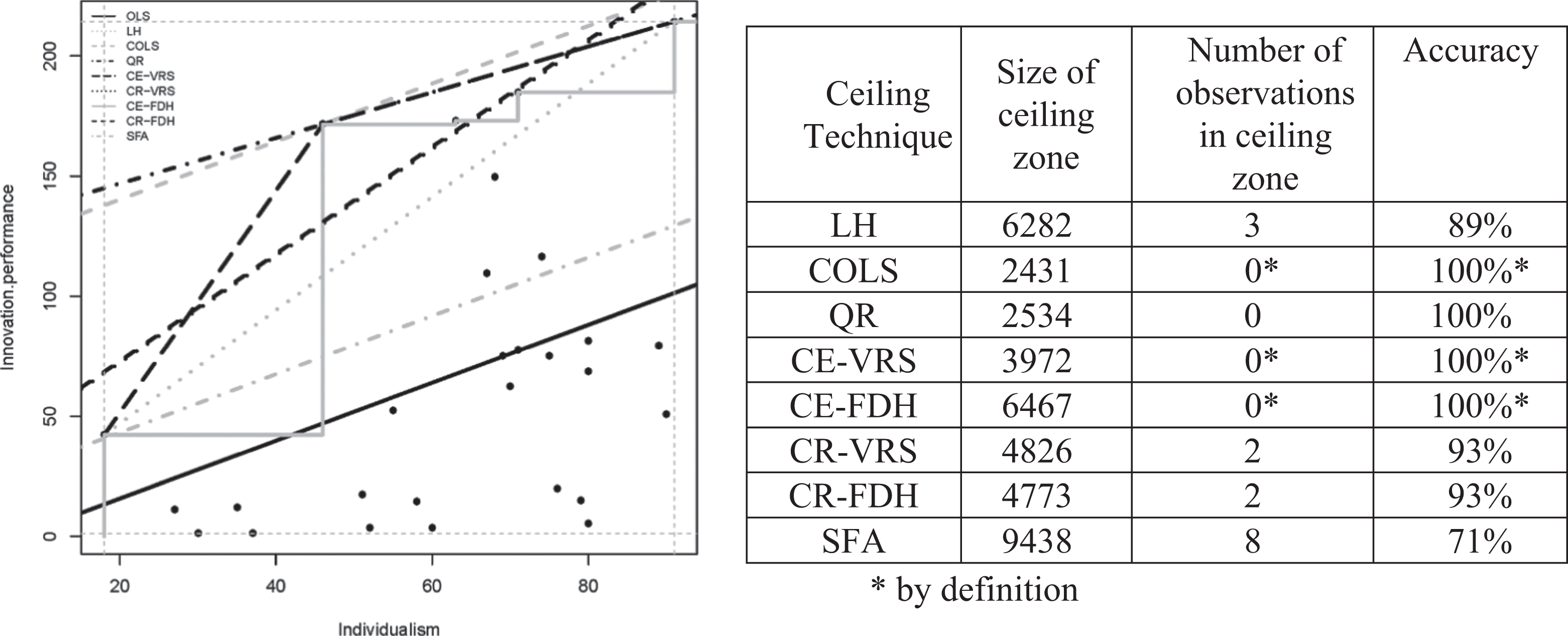
Application of different ceiling techniques to a data set on a country’s individualism (X axis) and its innovation performance (Y axis).
The scatterplot shows that there is an empty space in the upper left corner indicating the presence of a necessary condition: Individualism (X) is necessary for innovation performance (Y). The ceiling lines differ considerably across techniques. The techniques that use all 28 observations (i.e., COLS, quantile regression [QR], and SFA) seem to underestimate (COLS and QR) or overestimate (SFA) the size of the ceiling zone. From the remaining techniques that do not allow observations in the ceiling zone (CE-VRS and CE-FDH), CE-FDH defines a considerably larger ceiling zone than CE-VRS because it is not restricted by a convexity requirement. From the remaining techniques that allow observations in the ceiling zone and have a predefined (linear) ceiling line (LH, CR-VRS, CR-FDH), LH is less accurate than CR-VRS and CR-FDH but defines a larger ceiling zone. In this example, CR-VRS and CR-FDH result in virtually the same ceiling line. For reference, the OLS line is shown in Figure 5 as well (the lowest straight line). It is clear that a line through the middle of the data that describes an average trend is not a proper candidate for a ceiling line (accuracy in this example is only 64%).
Analyzing a number of empirical samples and using simulated data sets indicate that CE-FDH and CR-FDH generally produce stable results with relatively large ceiling zones and with no (CE-FDH) or few (CR-FDH) observations in the ceiling zone. CE-FDH is similar to Goertz et al.’s (2013) rectangular approach and produces a piecewise linear function with no observations in the ceiling zone; CR-FDH is a technique developed for the present purpose of NCA. It produces a smooth linear ceiling function with normally a few observations in the ceiling zone. The ceiling techniques presented here are only linear nondecreasing ceiling lines. In future work, also nonlinearities will be explored, for example, triangular or trapezoidal piecewise linear functions, or nonlinear functions such as polynomials or power functions. The quality of ceiling lines needs to be systematically compared by evaluating fit, effect size, accuracy, and required assumptions.
Effect Size of the Necessary Condition
Perhaps in nearly all scatterplots, an empty space can be found in the upper left corner, which may indicate the existence of a necessary condition if this makes sense theoretically. The question then is: Is the necessary condition large enough to be taken seriously? Therefore, there is a need to formulate an effect size measure. An effect size is a “quantitative reflection of the magnitude of some phenomenon that is used for the purpose of addressing a question of interest” (Kelley & Preacher, 2012, p. 140). Applied to necessary conditions, the effect size should represent how much a given value of the necessary condition Xc constrains Y. The effect size measure for necessity but not sufficiency proposed here builds on the suggestion by Goertz et al. (2013) that “the importance of the ceiling … is the relative size of the no observation zone created by … the ceiling” (p. 4). The effect size of a necessary condition can be expressed in terms of the size of the constraint that the ceiling poses on the outcome. The effect (constraint) is stronger if the ceiling zone is larger. Hence, the effect size of a necessary condition can be represented by the size of the ceiling zone compared to the size of the entire area that can have observations. This potential area with observations is called the scope (S). The larger the ceiling zone compared to the scope, the lower the ceiling, the larger the ceiling effect, the larger the constraint, and therefore the larger the effect size of the necessary condition. The effect size can be expressed as follows: d = C/S, where d is the effect size, 13 C is the size of the ceiling zone, and S is the scope. Hence, d is the proportion of the scope above the ceiling. The scope can be determined in two different ways: theoretically, based on theoretically expected minimum and maximum values of X and Y, and empirically, based on observed minimum and maximum values of X and Y. Thus: S = (Xmax – Xmin) × (Ymax – Ymin).
Similar to other effect size measures such as the correlation coefficient r, or R 2 in regression, this necessary condition effect size ranges from 0 to 1 (0 ≤ d ≤ 1). An effect size can be valued as important or not, depending on the context. A given effect size can be small in one context and large in another. General qualifications for the size of an effect as “small,” “medium,” or “large” are therefore disputable. If, nevertheless, a researcher wishes to have a general benchmark for necessary condition effect size, I would offer 0 < d < 0.1 as a “small effect,” 0.1 ≤ d < 0.3 as a “medium effect,” 0.3 ≤ d < 0.5 as a “large effect,” and d ≥ 0.5 as a “very large effect.” 14 Two recent papers with applications of necessary condition analysis have effect sizes between 0.1 and 0.3. One of these is in political science (Goertz et al., 2013), the other in business research (Van der Valk, Sumo, Dul, & Schroeder, 2015). In both papers, these effect sizes were considered as theoretically and practically meaningful. If a dichotomous classification is desired (e.g., for testing whether or not a necessary condition hypothesis should be rejected or for making an in kind qualification of the absence or presence of a necessary condition), I suggest to use effect size 0.1 as the threshold. Hence, an in kind necessary condition hypothesis in the continuous case (X is necessary for Y) is rejected if the effect size d is less than 0.1. A distribution of more than 150 continuous necessary conditions effect sizes from different studies indicates that roughly 50% of the effect sizes are small (d < 0.1), about 40% are medium (0.1 ≤ d < 0.3), and about 10% are large (0.3 ≤ d < 0.5). Very large effect sizes (d ≥ 0.5) can only be expected when the ceiling line is not a straight line (see the example in Figure 6).
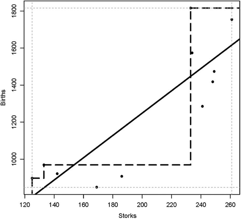
Scatterplot of the relation between the number of white storks nesting pairs in a region (Storks) during a given year and the number of human births during that year (Births).
The effect size of the dichotomous necessary condition, as shown in Figure 1, can be either 0 or 1. Without observations in the upper left hand cell, X is necessary for Y, and the effect size is 1. If there were observations in the upper left hand cell, X would not be necessary for Y, and the effect size would be 0. However, if there are only a few observations in the upper left cell in comparison to the total number of observations, two interpretations are possible. In the deterministic interpretation, X is still not necessary for Y. In the more flexible stochastic interpretation, which I adopt in this article, after evaluation of the outliers in the “empty” cell, X could be considered as necessary. Outliers can be “substitutes,” as in the example of the GRE score in Figure 1 (bottom), or can simply represent error. With a few outliers and depending on the context, one may decide to denote the condition as “virtually” necessary. No general rule exists about the acceptable number of cases in the “empty” upper left cell. Dul et al. (2010) suggest (arbitrarily) that a maximum number of 1 out of 20 observations (5%) is allowed in the “empty” cell. Hence, this decision rule is not based on effect size but on accuracy: Below 95% accuracy, the in kind necessary condition hypothesis in the dichotomous case is rejected. 15
In the dichotomous case, no other effect size values than 0 or 1 are possible. Yet, the left side of Figure 1 suggests that the ceiling zone equals 1 (one empty cell) and that the scope equals 4 (four cells with possible observations), hence that the effect size is one-fourth. This is incorrect. The actual effect size of the dichotomous case can be observed more easily from the right side of Figure 1. This figure shows that the scope equals 1 × 1 = 1. Also, the area of the empty space equals 1 × 1 = 1, and therefore the effect size is 1. Similarly, in the discrete case of Figure 2 without medium-medium observations, both the empty space and the scope would be (2 – 0) × (2 – 0) = 4, thus the effect size equals 1. With medium-medium observations, the scope would be (2 – 0) × (2 – 0) = 4, and the ceiling zone is (1 – 0) × (2 – 0) + (2 – 1) × (2 – 1) = 3, hence, the effect size is three-fourths (and not three-ninths as suggested by the left side of Figure 2). 16
In the example shown in Figure 5, the minimum and maximum observed values of X (18, 91) and Y (1.2, 214.4) result in an empirical scope of 15,563.6. Consequently, the effect size calculated with CE-FDH is 0.42, and the effect size calculated with CR-FDH is 0.31.
Necessity Inefficiency
The effect size is a general measure that indicates to which extend the “constrainer” X constrains Y, and the “constrainee” Y is constrained by X. However, normally, not for all values of X, X constrains Y, and not for all values of Y, Y is constrained by X. When the feasible space is triangular, as in Figure 3 (top left), X always constrains Y, and Y is always constrained by X. But when the feasible space is pentagonal, as in Figure 3 (top right), the ceiling line intersects the Y = YHigh axis and the X = XLow axis at other points than (XLow, YLow) and (XHigh, YHigh). As a result, for X > Xcmax, X does not constrain Y, and for Y < Ycmin, Y is not constrained by X. The upper left area between the lines X = Xcmax and Y = Ycmin in Figure 3 (top right) is the “necessary condition zone” where X always constrains Y and Y is always constrained by X. Within this zone, it makes sense to increase the level of the necessary condition in order to allow for higher levels of the outcome. Outside this zone, increasing the necessary condition level does not have such an effect. The area outside the necessary condition zone can be considered as “inefficient” regarding necessity. Necessity inefficiency has two components. Condition inefficiency (denoted here as i x) specifies that a level of resource/effort X > Xcmax is not needed even for the highest level of performance Y. 17 Condition inefficiency can be calculated as i x = (XHigh – Xcmax)/(XHigh – XLow) × 100% and can have values between 0 and 100%. Outcome inefficiency (i y) indicates that for a level of outcome Y < Ycmin, any level of X allows for a higher value of the outcome (e.g., higher performance ambition). Outcome inefficiency can be calculated as i y = (Ycmin – YLow)/(YHigh – YLow) × 100%, with values between 0 and 100%. The effect size is related to inefficiency as follows: d = ½ (1 – i x/100%) × (1 – i y/100%). The larger the inefficiencies, the smaller the effect size. When both inefficiency components are absent, the idealized situation of Figure 3 (top left) is obtained, and the effect size is 0.5, which is the theoretical maximum for a straight ceiling line. When one of the inefficiencies equals 100%, there is no ceiling, and thus no necessary condition and zero effect size. When the X and Y axes are standardized (e.g., XLow and YLow are 0 or 0% and XHigh and YHigh are 1 or 100%), the angle of the ceiling line is 45 degrees if both inefficiencies are equal. When condition inefficiency is larger than outcome inefficiency, the ceiling line is steep (>45 degrees). A slope that is less steep (<45 degrees) indicates that outcome inefficiency is larger than condition inefficiency. In Figure 3 (bottom left), the condition inefficiency is 33%. This means that for an Ambition level (X) above 67% of 100 = 67, Ambition is not necessary for even the highest level of Sales Ability. In Figure 3 (bottom left), outcome efficiency is 46%. This means that for a desired Sales Ability level (Y) that is below 46% of 5.5 (the maximum observed level) = 2.5, Ambition is not necessary for Sales Ability. Because outcome inefficiency (46%) is larger than condition inefficiency (33%), the slope of the ceiling line is less than 45 degrees. 18
Comparison of NCA with QCA
Multicausal phenomena can also be analyzed with other approaches that use the logic of necessity and sufficiency. For example, qualitative comparative analysis (Ragin, 2000, 2008; for an introduction, see Schneider & Rohlfing, 2013) is gaining growing attention in organizational sciences (Rihoux, Alamos, Bol, Marx, & Rezsohazy, 2013). It aims to find combinations of determinants that are sufficient for the outcome while separate determinants may not be necessary or sufficient for the outcome (Fiss, 2007). NCA and QCA are similar in the sense that they both approach causality in terms of necessity and sufficiency and not in terms of correlation or regression. However, two major differences are that NCA focuses on (levels of) single determinants (and their combinations), whereas QCA focuses on combinations of determinants (configurations), and that NCA focuses on necessary determinants that are not automatically sufficient, whereas QCA focuses on sufficient configurations that are not automatically necessary (equifinality with several possible causal paths). 19 Although QCA centers on sufficient configurations, it is also used for necessary condition analysis (e.g., Ragin, 2003). But the QCA approach for “continuous” necessary condition analysis (fuzzy set QCA) is fundamentally different than the NCA approach presented here (Vis & Dul, 2015). Instead of a ceiling line, QCA uses the bisectional diagonal through the theoretical scope as the reference line for evaluating the presence of a necessary condition. Thus, QCA presumes that necessary conditions are only present in triangular scatter plots. 20 If all observations are on and below the diagonal, the QCA reference line is the same as the NCA ceiling line. However, when a substantial number of data points show up above the reference line (e.g., because of inefficiencies, see examples in Figure 3 [top right and bottom] and in Figure 4), NCA “moves the ceiling line upward,” possibly with rotation, while the QCA reference line remains the same (the diagonal). Then NCA concludes that X is necessary for Y at lower levels of X, whereas QCA concludes that X is “less consistent” with necessity (necessity “consistency”; Bol & Luppi, 2013; Ragin, 2006) without specifying values of X where X is necessary for Y or where X is not necessary for Y. As a consequence, QCA normally finds considerably less necessary conditions in data sets than NCA Dul (2015a). Another difference is that QCA only analyzes in kind necessary conditions (condition X is necessary for outcome Y), whereas NCA can also analyze in degree necessary conditions (level of X is necessary for level of Y). NCA and QCA are also different with respect to evaluating the “importance” of a necessary condition. In NCA, importance is defined as the size of the empty zone in comparison to the scope, whereas in QCA (and other analytic approaches; e.g., Goertz, 2006a 21 ), importance of a necessary condition is defined as the extent to which the necessary condition is also sufficient (necessity “coverage”). In this view, a necessary condition is more important if it is more sufficient. 22 However, a fundamental notion in the current article is that single organizational ingredients are not sufficient for multicausal organizational phenomena, which explains and justifies the necessary but not sufficient expression. For a further discussion on the differences between NCA and QCA, see Vis and Dul (2015) and Dul (2015a).
Applying NCA instead of QCA for analyzing necessity can result is different conclusions. For example, Young and Poon (2013) applied QCA to identify the necessity of five IT project success factors: top management support, user involvement, project methodologies, high-level planning, and high-quality project staff. Using a sufficiency view of importance of necessity (Goertz, 2006a), they found importance levels of 0.97, 0.64, 0.70, 0.69, and 0.61, respectively. Applying the NCA approach to Young and Poon’s data set using CE-FDH gives necessary condition effect sizes of 0.30, 0.25, 0.19, 0.33, and 0, respectively. Comparing the rank orders of these two approaches shows that top management support is the most important in the sufficiency view, followed by project methodologies and high-level planning. However, in the necessary but not sufficient view, high-level planning has the largest effect size, followed by top management support and user involvement. The bottleneck analysis indicates that only project methodologies is necessary for a medium success level of 0.5 (the observed success levels ranged from 0.1 to 0.9), and the other four determinants are not. Yet, if the desired level of success increases, more conditions become necessary, and four out of five conditions are necessary for the maximum observed outcome level (0.9), with required levels of the five determinants of at least 88%, 67%, 25%, 100%, and 0% of the maximum range of observed levels of these determinants, respectively (the last determinant is not necessary). These percentages show necessity inefficiencies for all four determinants that are necessary, except for high-level planning that needs a level of 100% for maximum outcome. This NCA analysis adds to Young and Poon’s insights that top management support “is significantly more important for project success than factors emphasized in traditional practice” (p. 953). The NCA analysis shows that top management support is needed if maximum performance is desired, but not at maximum level. Top management support is not needed if only medium performance is desired (then project methodologies is needed). More importantly, for maximum performance, adequate levels of the other determinants, which Young and Poon call the “factors emphasized in traditional practice,” are also needed. Hence, high outcomes will not occur without properly balancing the minimum levels of the four necessary determinants. Therefore, NCA analysis does not support Young and Poon’s conclusion that “current practice emphasizing project methodologies may be misdirecting effort” (p. 953) because considerable levels of four necessary determinants including project methodologies are needed for high performance. This example of an additional NCA analysis is presented for purposes of illustration, and it is typical for the necessary but not sufficient approach. It may provide new insights about how organizations can efficiently put and keep organizational ingredients in place to achieve a desired outcome and by which level.
Limitations of NCA
Just like any other data analysis approach, NCA has several limitations. One fundamental limitation that it shares with other data analysis techniques is that NCA cannot solve the problem of “observational data cannot guarantee causality.” Observational studies are widespread in organizational research. All examples in Table 1 and all the examples used for illustration in this article are from observational studies. Observing a data pattern that is consistent with the causal hypothesis is not evidence of a causal connection. Hence, it is important that identified necessary conditions are theoretically justified, namely, that it is understood how X constrains Y and Y is constrained by X. Requirements for causal inference in empirical studies for building or testing necessary cause-effect relations are the same as for any other type of cause-effect relation. For example, a necessary cause is more plausible if the cause precedes the outcome and is related to the outcome and if an observed outcome cannot be explained by another cause (Shadish et al., 2002). If such requirements are not met, a necessary condition outcome that is empirically observed may, for example, be spurious, namely, caused by another variable (Spector & Brannick, 2010). This can be illustrated with a revision of the classic example of the relation between the number of storks in a region and the number of human newborns in that region (Box, Hunter, & Hunter, 1978). 23 Figure 6 shows a scatterplot of the relationship between the annual number of white stork nesting pairs and the number of human births in the Oldenburg region in Germany over one decade. The scatterplot shows that there is an empty area in the upper left corner. The ceiling line is drawn with the CE-FDH rather than with the CR-FDH ceiling technique because the observations along the border between the empty zone and the full zone cannot be well represented by a straight line.
The data suggest the existence of a necessary condition with a very large effect size (0.73): A high number of human births in the region is only possible if the number of stork nesting pairs in the region is large. It is clear (unless one believes in fables or in the Theory of the Stork; Höfer & Przyrembel, 2004) that a theoretical explanation is missing in this example. A necessary relationship that is observed between X and Y can be spurious if a variable Z is sufficient for X and necessary for Y (Mahoney, 2007). In the storks example, one could state that when more people (Z) settle in a region and build houses with chimneys and other high human-made constructions, the number of stork nesting pairs (X) increases because storks favor high nesting places: Z produces X, hence is a sufficient cause of X. Additionally, Z is a necessary cause of Y because a high increase of the number of births is only possible when there are more people. In other words, the variable Z is the reason of the presumed “necessary” relation between storks and births. 24 This example shows again that without theoretical support, a necessary condition cannot be presumed from observational data. This is not different from any other data analysis approach using observational data.
If the cause can be manipulated, a research design based on randomized experiments may be better equipped to fulfill requirements for causality than an observational study. A potential necessary cause of a multicausal phenomenon (e.g., storks for birth) can be tested in a randomized experiment where instances (cases) with the cause (regions with storks) are selected randomly from a defined population (all regions with storks) and then randomly assigned to the experimental group (regions that get a treatment) or control group (regions that do not get a treatment). In the experimental group, the presumed necessary causal condition is manipulated by taking it away (e.g., storks are chased away), whereas in the control group, the presumed causal condition is unchanged. Then we observe whether the effect disappears in the experimental group (reduction of birth rate) but not in the control group (birth rate constant). Such a design provides strong evidence for the (non)existence of a necessary cause. This type of experiment contrasts the common “sufficiency” experiment in which first cases without the cause (regions without storks) are randomly selected from a population (all regions without storks) and randomly assigned to the experimental or control group. Then the cause is added to the experimental group (storks are introduced), and we observe if the effect appears in the experimental group (increase of birth rate) and not in the control group (birth rate constant). 25 The necessity experiment can be rephrased as a sufficiency experiment because a necessary condition that is formulated as “the presence of the cause is necessary for the presence the effect” can also be formulated as “the absence of the cause is sufficient for the absence of the effect.” Then in the sufficiency approach for testing a necessary cause, the “absence of the cause” (no storks) is added to the experimental group and we observe if the “absence of the effect” (reduction of births) appears. If the necessary cause cannot be manipulated (cannot be taken away), nonexperimental research designs such as natural experiments (where the necessary cause disappears naturally, and we observe if the effect disappears) or observational studies (where we observe if the necessary cause is present in cases with the effect or if the effect is absent in cases without the necessary cause) can be applied. Such approaches rely more on solid theoretical reasoning in order to infer necessity causality.
A limitation of NCA is that it may be more susceptible for sampling and measurement error than traditional data analysis approaches. The reason is that the proposed ceiling techniques (CE-FDH and CR-FDH) only use a small proportion of the observations in the sample for drawing the ceiling line (the observations near the ceiling line). The ceiling line (and therefore other quantities derived from it, e.g., effect size, accuracy) may be sensitive to selection bias and measurement error in the cases around the ceiling line. This particularly holds if the number of cases around the ceiling line is relatively small. Therefore, the accuracy of the ceiling line depends on having representative cases around the ceiling line with accurate measurement of the variables. Measurement precision and validity need to be ensured, in particular for the cases that are expected to be around the ceiling line (e.g., relatively successful cases). The ceiling line may also be susceptible to exceptions, outliers, or counterexamples in the upper left corner of the scatterplot. Therefore, observations near the ceiling line need to be evaluated before conclusions can be drawn. Exceptions (high outcome without the necessary condition) may be due to measurement error, unexplained stochasticity in the data, the case not being part of the theoretical domain where the necessary theory is supposed to hold, or the existence of a substitute condition that reflects the underlying concept (see example of Figure 1 [bottom] where GRE score and opinion of faculty member both indicate a student’s quantitative ability). The evaluation of cases near the ceiling line is not only desirable for reasons of internal validity; it also gives insight in “peers,” “best practices,” or “most efficient” cases. Cases near the ceiling line have the highest outcome in comparison with other cases with the same level of the necessary condition. These cases are therefore most efficient in the sense that they have the highest possible outcome for the given level of the necessary condition (outcome efficiency) and the lowest possible level of the necessary condition for the given outcome (condition efficiency).
NCA is a data analysis tool for calculating ceiling lines, effect sizes, and other relevant quantities. If the researcher is only interested in the specific data set, without a need for generalization to a wider population, this is perfectly acceptable. Also, if the data set is a census (all members of the population are in the data set), the calculated quantities are true representations of the population. However, if for reasons of statistical inference the data set is a probability sample from a population, the NCA quantities are only point estimates. Currently, NCA does not take sampling error into account (e.g., the NCA estimates have no confidence intervals). Future research could focus on adding confidence intervals to point estimates of NCA parameters. Building on developments within the field of production frontiers estimation, such confidence intervals could be based on resampling approaches such as jackknifing and bootstrapping (e.g., Simar & Wilson, 1998) or on Bayesian approaches (e.g., Pendharkar & Pai, 2013). Another sampling related limitation is introduced if purposive sampling is applied. Purposive sampling is an efficient way to select samples for calculating NCA quantities (see the example of selecting successful cases in Appendix A). The intention is that the sample is representative only for cases that are around the ceiling line (relatively successful cases). Then, relatively unsuccessful cases are not well represented in the sample, and therefore general sample descriptives (e.g., mean values of variables) or average sample trends (regression) do not represent the whole population. It should also be noted that a necessary condition may be trivial. When in a data set obtained by purposive or random sampling a necessary condition is identified, it is possible that this condition is trivial. Trivialness is the extent to which observations, on average, are clustered toward the maximum value of the necessary condition; hence, low values of the condition are rare. For example, if the required GRE score for admission would be for example 200, virtually all students would reach that score. Then such score would still be necessary for admission, but it would be trivial because a score below 200 hardly exists. Similarly, references are necessary for an impactful paper in ORM, but this condition is trivial because nearly all papers have references. A check on trivialness requires the identification of the existence of cases without (or with low levels of) the necessary condition (Dul et al., 2010).
Recommendations for Applying NCA
NCA can be applied in any branch of organizational research (and elsewhere) in which theoretical necessary (but not sufficient) statements are (or can be) formulated. Table 1 gives examples of such statements in strategy, organizational behavior, and human resource management. Also, many examples exist in other organizational research fields such as operations management (Dul et al., 2010; McLachlin, 1997; Van der Valk & Wynstra, 2012; Van der Valk et al., 2015) and business history (Westerhuis, Dul, De Jong, & Hak, 2012), in other social sciences including political science (Goertz, 2003), and even beyond that in medical and technical sciences. 26 The examples show that depending on the focal unit of the theory, necessary conditions can be formulated at any organizational level: individual, team, project, work unit, business unit, firm, country, and so on. What is common in these formulations is that the necessary condition is a nontrivial characteristic, event, resource, or effort that is relatively unique, scarce, or costly and that must be designed, controlled, or managed to bring or keep it in place in order to allow a certain desired outcome to occur. Without the necessary condition, there is guaranteed failure of that desired outcome. One may expect to find necessary conditions in data sets with variables that are plausibly causally related because it seems rare that a desired outcome occurs for free, hence without keeping in place a nontrivial, unique, scarce, or costly condition. Therefore, I recommend that researchers should always search for necessary conditions in data sets with presumed causal relations between X and Y and to acknowledge that necessary causes are different from sufficient causes and that traditional data analysis techniques (correlation, regression) focus on sufficiency, whereas NCA focuses on necessity. The NCA analysis may complement (e.g., precede) traditional analyses.
Just like traditional data analysis techniques, NCA is a data analysis technique and not a data collection and measurement technique. It assumes that the scores of X and Y are reasonably valid (i.e., measurement instruments measure what they intended to measure) and reliable (precise). Current techniques to check the quality of measurements may be applied. It also assumes that the basic requirements to make it plausible that X can cause Y are met (e.g., X preceeds Y). Furthermore, the instances (cases) in the database are considered to represent the group of instances (cases) that is of interest to the researcher, namely, a specific group of instances (cases) with certain characteristics, a representative sample obtained by probability sampling from a population of interest, or a census of a population of interest.
Building on suggestions provided in Dul et al. (2010), I recommend the following: Recognize that traditional analysis (correlation, regression, “average line through the middle”) and necessary conditions analysis (ceiling line) are fundamentally different and equally valid for their own purposes. Recognize that the managerial relevance of a necessary condition analysis (without X there is guaranteed failure of Y, and this cannot be compensated by other determinants) might be stronger and more relevant for practical decision making than that of a traditional analysis (more X on average results in more Y). Recognize that it is not uncommon that necessary conditions exist in data sets, although effect sizes may vary. Recognize that when traditional data analyses do not show strong traditional relationships, there still may be strong necessary conditions (see example of Figure 4). Do not formulate theoretical necessary condition statements (X is necessary for Y or X is necessary but not sufficient for Y) as traditional hypotheses (e.g., X affects Y), as was done in the examples in Table 1. Test necessary condition hypotheses with NCA, not with traditional analysis (correlation, regression), as was done in the examples in Table 1. Formulate results of a traditional analysis in traditional terms, not in terms of necessary conditions, as was done in the examples in Table 1. Formulate results of a necessary condition analysis in necessary condition terms, not in traditional terms (see Dul et al., 2010, for examples).
In the following, I provide some extended recommendations for researchers wanting to use NCA to analyze their data. These recommendations focus on (1) performing a data analysis with NCA and (2) reporting NCA results. Finally, I describe a software tool for conducting NCA.
Recommendations for Performing a Data Analysis With NCA Using a Stepwise Approach
Tables 3 and 4 show six steps for performing a necessary condition analysis. Table 3 refers to a situation where both X and Y are continuous variables or discrete variables with a large number (e.g., >5) of variable levels. Then the analysis is illustrated with a scatterplot as in Figures 3, 4, 5, and 6. Table 4 refers to a situation where both X and Y are dichotomous variables or discrete variables with a small number (e.g., <5) of variable levels. Now the analysis is illustrated with a contingency table as in Figures 1 and 2. Steps 1 and 2 and Steps 5 and 6 are relatively easy in both the scatterplot approach and the contingency table approach. Step 3 (draw ceiling line) and Step 4 (quantify NCA parameters) are relatively easy in the contingency table approach but more complex in the scatterplot approach. The NCA software tool has been developed (see the following) to assist in performing these steps. All steps in the contingency table approach can be performed by “manual/visual” analysis of the contingency table. This is particularly easy when the number of levels of the discrete variables is relatively low. The analysis for situations with dichotomous variables or discrete variables with a small number (e.g., <5) can also be done with the NCA software. Then the alternative data visualization with a Cartesian coordinate system (as in the right sides of Figures 1 and 2) and the scatterplot approach with the CE-FDH ceiling line technique must be used. This alternative analysis with NCA software (Table 3) gives the same results as the manual/visual contingency table approach (Table 4).
Stepwise Approach for Data Analysis With Necessary Condition Analysis (NCA) for Continuous and Discrete Variables With a Large Number of Levels (Scatterplot Approach).
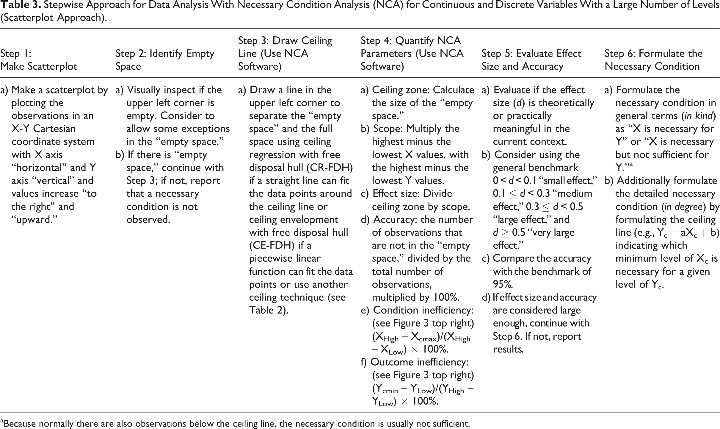
aBecause normally there are also observations below the ceiling line, the necessary condition is usually not sufficient.
Stepwise Approach for Data Analysis With Necessary Condition Analysis (NCA) for Dichotomous and Discrete Variables With a Small Number of Variable Levels (Contingency Table Approach).
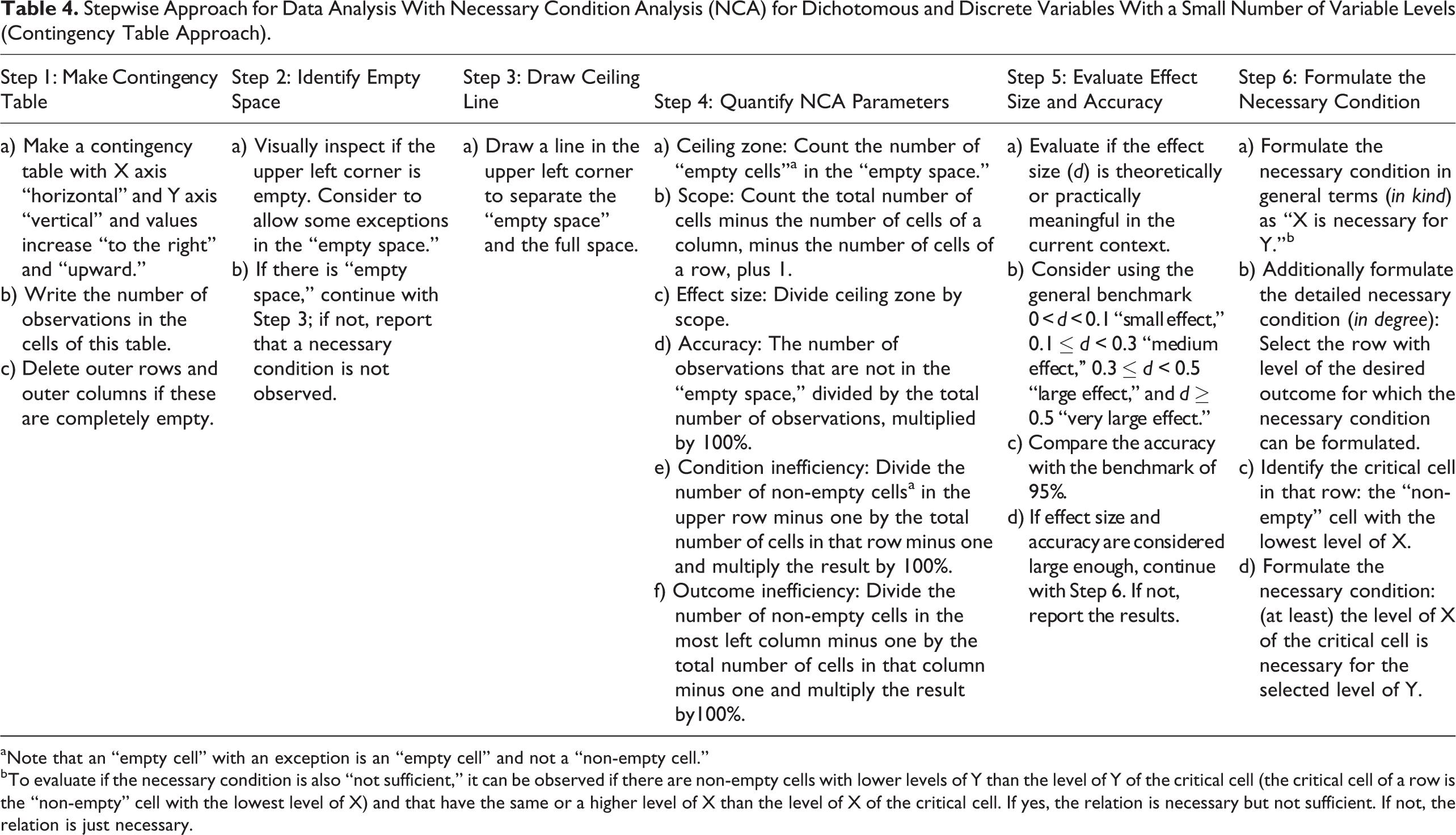
aNote that an “empty cell” with an exception is an “empty cell” and not a “non-empty cell.”
bTo evaluate if the necessary condition is also “not sufficient,” it can be observed if there are non-empty cells with lower levels of Y than the level of Y of the critical cell (the critical cell of a row is the “non-empty” cell with the lowest level of X) and that have the same or a higher level of X than the level of X of the critical cell. If yes, the relation is necessary but not sufficient. If not, the relation is just necessary.
Recommendations for Reporting NCA Results
In addition to the common standards for reporting research results, specific elements need to be added for describing the details of a necessary condition analysis. When a necessary but not sufficient theoretical statement is made, it is recommended that researchers should consistently formulate the theory to be tested or built as a necessary (but not sufficient) causal theory (e.g., by formulating propositions/hypotheses in terms of X is necessary [but not sufficient] for Y or by formulating a research question to which extend X is necessary but not sufficient for Y). Contrary to common practice (see Table 1), such theoretical statements should not be formulated (implicitly) as a sufficiency theory (e.g., by formulating traditional general propositions/hypotheses such as X affects Y or X has a positive effect on Y). In the Methods section of the report, it can be stated that a necessary condition analysis was applied to evaluate (test) or formulate (build) a necessary but not sufficient theoretical statement, and it could be specified how the six steps (Table 3 or 4) were performed. In the scatterplot approach, the specific ceiling technique (e.g., ceiling regression or ceiling envelopment) needs to be specified. Also, specification of the criteria for evaluation of the practical or theoretical significance of the effect size of the necessary condition is required. If specific criteria for the study’s specific context are not feasible, the general benchmark for necessary condition effect size may be selected (i.e., 0 < d < 0.1 “small effect”, 0.1 ≤ d < 0.3 “medium effect,” 0.3 ≤ d < 0.5 “large effect,” and d ≥ 0.5 “very large effect”), and for a dichotomous classification, an effect size threshold of 0.1 could be used. In the Results section of the report, first the contingency table or the scatter plot (including ceiling line) could be provided. Next an NCA results table with basic information about the NCA parameters (Step 4 in Tables 3 and 4) could be formulated for each necessary condition. As a minimum, this table should include: ceiling zone, scope, effect size, and accuracy. For discrete and continuous necessary conditions, also condition inefficiency and outcome inefficiency could be included. Table 5 shows the NCA results tables of the three illustrative examples in this article. In these examples, the general benchmark for effect size is used to appraise the results (see the asterisks). If the effect size is considered large enough, the necessary condition can be formulated in kind: X is necessary for Y. Subsequently, the ceiling line or bottleneck table can be used to formulate the necessary condition in degree: Level of X is necessary for level of Y.
Necessary Condition Analysis (NCA) Result Tables for the Three Illustrative Examples.
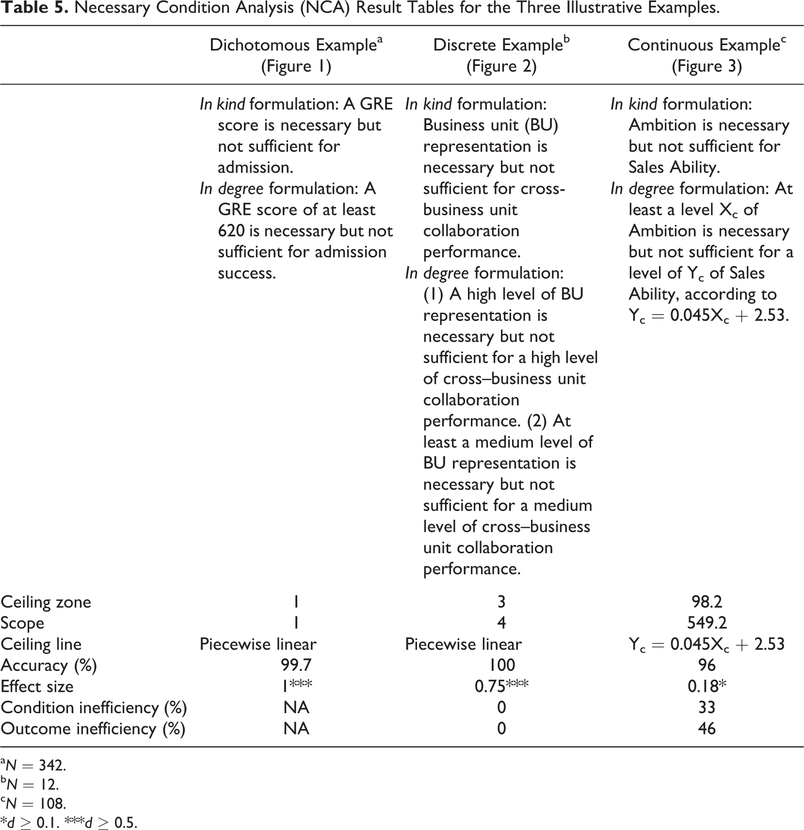
a N = 342.
b N = 12.
c N = 108.
*d ≥ 0.1. ***d ≥ 0.5.
Additionally, the bottleneck table can be provided, in particular in the multivariate situation, showing which levels of the condition is a bottleneck for certain desired levels of the outcome. Figure 3 (bottom right) and Figure 4 (lower part) give examples of such tables. For convenience to the readers, the researcher can interpret the bottleneck table and the ceiling line as follows. First the researcher can classify the outcome (first column of the bottleneck table) into several classes, for example three classes (low, medium, and high outcome) on the basis of theoretical or practical considerations, measurement scale values (e.g., for a 7-point Likert scale low, <3; medium, 3-5; high, >5), the statistical distribution of the data (e.g., low, <25th percentile; medium, 25th-75th percentile; high, >75th percentile), or the structure of the data. Then for each class it can be indicated how many and which levels of determinants are required to allow that outcome. For example in Figure 4, based on the structure of the data, three classes are distinguished. In the low range outcome values (<50%), no determinant is necessary. In the middle outcome values (50%-60%), some but not all determinants are necessary and their levels need to be up to 20%. In the high range with outcome >70%, all four determinants are necessary for a high outcome with required condition levels of 15% to 73%. For the highest outcome (100%), all determinants must have a value of least 50% (and one nearly 100%). When the required condition percentage is below 100%, there is condition inefficiency.
A Software Tool for Necessary Condition Analysis
An NCA software tool is made available to identify necessary conditions in data sets. The tool was developed to facilitate the process of drawing ceiling lines, calculating NCA parameters, and creating bottleneck tables. The software, called NCA, is a package that runs with open source programming language R (Culpepper & Aguinis, 2011). The software can be obtained freely from http://cran.r-project.org/web/packages/NCA/index.html (Dul 2015b). A quick start guide is available at http://ssrn.com/abstract=2624981 or http://repub.eur.nl/pub/78323/ (Dul 2015c), which allows novice users without knowledge of R or NCA to perform an analysis within 15 minutes.
The NCA package does three main things: It draws NCA plots, which are scatter plots with ceiling lines. The user can select up to eight different ceiling line techniques presented in Table 5. The defaults are CE-FDH (piecewise linear function) and CR-FDH (straight line). It calculates the NCA parameters: ceiling zone, scope, accuracy, effect sizes, condition inefficiency, and outcome inefficiency for each selected ceiling technique. The default scope is the empirical scope calculated from the minimum and maximum values of X and Y in the data set. It calculates the values of variables in the bottleneck table to analyze which X is the bottleneck for a given Y.
The output includes scatterplots with ceiling line(s), a table with the NCA parameters (as well as other relevant information), and the bottleneck table. For running the NCA package, the user can change several parameters to fit the software to the specific situation.
Conclusion
This article presents the necessary but not sufficient interpretation of X causes Y. Such statements are common in the organizational sciences (and beyond), but the traditional correlation- and regression-based data analysis frameworks and tools do not fit such interpretations. The necessary condition analysis methodology provides a solution. It is new in the organizational sciences and is particularly useful in situations with multicausality in which several known and unknown determinants (e.g., events, characteristics, resources, efforts) contribute to a desired outcome (e.g., good performance) but none is sufficient. In such situations, the proposed new approach can identify the “critical” (levels of) determinants that are necessary for achieving the outcome and that must be put and kept in place in order to make it possible to achieve the desired outcome. Therefore, organizational researchers are encouraged to apply NCA methodology to their research and data sets. Scatterplots that show heteroskedasticity, or relatively low average effects of X on Y, are no reasons for not applying NCA: In such situations, X might be necessary but not sufficient for Y. With the NCA approach and the freely available NCA software, it is relatively easy to perform such analyses. It may bring new insights to organizational phenomena.
Footnotes
Appendix A: Necessary Ingredients of a Caesar Salad
Imagine a novice cook planning to prepare a classic Caesar salad. 27 A quick look at recipes reveals that such a salad must have Parmesan cheese. A salad without Parmesan is not a Caesar salad. But a salad with Parmesan does not make it a Caesar salad; Parmesan is necessary but not sufficient for a salad being classified as a Caesar salad. Other ingredients (croutons, romaine lettuce) are necessary as well, but ingredients such as chicken or bacon are not always added and just contribute to some Caesar salads. A single necessary ingredient or the set of identified necessary ingredients are not sufficient for the outcome, but they increase the probability of success. However, not using the necessary ingredients will result in guaranteed failure.
How can a novice cook find out which ingredients define a Caesar salad? A traditional approach to answer this question implies an analysis of a large sample of salad recipes in which ingredients are determinants and a Caesar salad or not is the outcome. A Google search on January 10, 2014, with the keywords recipes and salad resulted in more than 150 million hits. The 82nd hit was the first Caesar salad. Hence a large N would be required to perform a regression analysis for estimating the contribution of the observed ingredients to the outcome of yes/no Caesar salad. The necessary condition analysis (NCA) approach, on the other hand, can do purposive sampling of cases on the basis of the presence of the outcome (Caesar salad). It evaluates which ingredients are present in these cases. Using the keywords recipe, Caesar, and salad results in more than 3 million hits, and for simplicity I analyzed only the first 10 hits, which all were recipes of Caesar salads. This resulted in the main ingredients presented in Table 6.
It turns out that Romaine lettuce, croutons, and Parmesan are present in these recipes of Caesar salad. Hence these ingredients are candidate necessary conditions: The outcome (Caesar salad) is not possible without them. Anchovy is included in nearly all Caesar salads except for case 6 where it is optional, hence it is virtually necessary. The other ingredients (bacon, chicken) are not necessary: The outcome (Caesar salad) is possible without them. Having the identified necessary ingredients in place will result in a larger probability that the outcome will be a Caesar salad. This can be illustrated as follows. Entering the words recipe and salad together with one necessary condition (Romaine lettuce, croutons, or Parmesan) in a Google search resulted for the first 10 hits in 0, 1, and 0 recipes of Caesar salad, respectively; hence, the average probability that with one necessary ingredient in place a salad is a Caesar salad is 1/30 = 0.03. When two ingredients are in place, the search with the three possible combinations of two necessary ingredients resulted in an average probability of 0.33 that the salad is a Caesar salad, and with all three ingredients in place, the probability that recipes with this set of necessary ingredients results describe a Caesar salad is 0.90 (9 of the 10 first hits were Caesar salads). When including anchovy as a “virtually necessary ingredient” (when allowing some stochasticity), all first 10 hits were Caesar salads (the 13th hit was not a Caesar salad). This example shows that it is relatively easy to find necessary but not sufficient conditions in data sets by focusing on the conditions that are common in cases with high outcome and that the probability of the high outcome increases when more necessary conditions are in place but the set of identified necessary conditions is not automatically sufficient for the outcome.
Appendix B: Necessary Conditions for Successful Business Unit Collaboration
Martin and Eisenhardt (2010) analyzed success of collaboration between business units in multi-business firms. Table 7 summarizes the data of the 12 cases (collaborations) in this study. From interviews with corporate and business unit informants, the authors obtained discrete (mainly dichotomous and trichotomous) scores for collaboration performance (variables P1-P2) and presumed determinants of collaboration success (variables D1-D11).
The table shows, for example, that determinant “origin of the collaboration” (determinant D1) is scored at two levels (H = business unit, L = corporate) and that determinant business unit representation, which is the extent to which all relevant business units are represented in the collaboration team (determinant D8) is scored at three levels: H = high representation, M = medium representation, and L = low representation. For their purposive sampling strategy, the authors initially scored the outcome variable (performance in terms of collaboration success) dichotomously (H = high performing, L = low performing) based on preliminary interviews with a firm’s corporate executive (performance measure P1). Afterward, collaboration performance was rated by corporate executives using an 11-point scale from 0 = unsuccessful, to 5 = moderately successful, to 10 = highly successful (performance measure P2). For illustration purposes, I trichotomized these performance scores such that scores 0, 1, 2, 3 reflect “low” collaboration performance; scores 4, 5, 6, 7 “medium” performance; and scores 8, 9, 10 “high” performance (performance measure P3).
Table 8 (middle column) shows potential necessary but not sufficient conditions that can be easily derived from Table 7 by visual inspection: looking at the common determinants in successful cases. These hypotheses were not identified by the authors. Instead, they derived traditional sufficiency-based hypotheses, namely, that the determinant “is more likely to yield” a high outcome (Table 8, right column).
Acknowledgments
I would like to thank Gary Goertz and Tony Hak, as well as Ioannis Evangelidis, Roelof Kuik, Erik van Raaij, Daan Stam, Regien Sumo, Wendy van der Valk, and Barbara Vis, for their constructive comments on earlier versions of this paper. I am grateful to Jeffrey Foster for providing me the data of the Hogan Personality Inventory (HPI) example and to Hans van Maanen for the data on the storks example. I wish to thank the three anonymous reviewers for their valuable comments and James LeBreton for his helpful guidance as acting editor.
Declaration of Conflicting Interests
The author(s) declared no potential conflicts of interest with respect to the research, authorship, and/or publication of this article.
Funding
The author(s) received no financial support for the research, authorship, and/or publication of this article.