Sage Journals: Discover world-class research

Abstract

We implement and analyse a sparse/indirect-addressing data structure for the Lattice Boltzmann Method to support efficient compute kernels for fluid dynamics problems with a high number of non-fluid nodes in the domain, as encountered in porous media flows. The data structure is integrated into a code generation pipeline to enable sparse Lattice Boltzmann Methods with a variety of stencils and collision operators and to generate efficient code for kernels on CPU as well as on AMD and NVIDIA accelerator cards. To further enhance performance, we optimize these sparse kernels with an in-place streaming pattern to save memory accesses and memory consumption and we implement a communication hiding technique to demonstrate strong scalability. We provide a comprehensive, systematic performance analysis comparing the sparse and the traditional dense data structure. We present single GPU performance results for the sparse approach with up to 99% of maximal bandwidth utilization. We integrate the optimized generated kernels in the high performance framework waLBerla and achieve a scaling efficiency of at least 82% on up to 1024 NVIDIA A100 GPUs and up to 4096 AMD MI250X GPUs on modern HPC systems. In addition, we propose a hybrid data structure that enables an adaptive choice between sparse and dense representations on a per-subdomain basis, allowing further improvements in performance and memory efficiency. We evaluate all approaches on three realistic application scenarios: flow through porous media, free flow over a particle bed, and blood flow in a coronary artery. Across these benchmarks, we demonstrate a speed-up of up to 2x and a reduction in memory consumption of up to 75% using the sparse/indirect-addressing data structure compared to the conventional direct-addressing approach.

Keywords

sparse lattice Boltzmann method indirect addressing complex geometries high performance computing GPU computing large scale porous media

1. Introduction

The increasing power of high-performance computing (HPC) systems enables computational fluid dynamic (CFD) simulations, which were still out of scope some years ago. The leading HPC systems in the Top500 list¹ reach a peak performance of ExaFLOPs, so they can perform 10¹⁸ floating point operations per second. This trend is also caused by the utilization of accelerators, such as NVIDIA, AMD, or INTEL Graphics Processing Units (GPUs). With these new computing capabilities, computational fluid dynamic (CFD) problems, which were out of scope before, can now be tackled, such as fully resolved porous media simulations at relevant scales, as presented in Mattila et al. (2016) or entire body arterial flows as in Randles et al. (2015). However, it is not trivial to fully utilize the maximum performance of these HPC systems, especially for systems with accelerators (Brodtkorb et al. (2013); Hijma et al. (2023); Lai et al. (2020); Rak (2024)).

The Lattice Boltzmann method (LBM) (Chen and Doolen (1998); Qian et al. (1992)) is an efficient inherently parallel method to solve CFD problems for complex geometries. On many HPC systems, the LBM shows excellent performance as presented in Liu et al. (2023), Spinelli et al. (2023), Watanabe and Hu (2022) or Godenschwager et al. (2013).

There are two common ways to store data for LBM simulations. The direct-addressing LBM stores and computes all cells of the domain. We call this technique “dense” or ”direct-addressing” data structure in the following.

It is shown to be very fast and efficient for most simulation setups and therefore used for example in the LBM frameworks Palabos (Latt et al. (2021)), ProjectPhysX (Lehmann et al. (2022)), Sailfish (Januszewski and Kostur (2014)) and OpenLB (Krause et al. (2021)). However, the direct-addressing data structure struggles in performance and memory consumption for simulation domains with a high number of non-fluid nodes, such as in porous media flows. In the following, we call such domains “sparse domains”. In contrast, simulations with a high percentage of fluid nodes, such as a free channel flow, we will refer to as “dense domain”.

The second way to store data for LBM simulations is the indirect-addressing storage format. We call it “sparse” data structure in the following. This approach stores only fluid cells and can therefore save a significant amount of memory. Additionally, the sparse approach reaches superior performance for sparse complex geometries as compared with the dense approach. Therefore, it is used in multiple LBM frameworks such as HARVEY (Randles et al. (2013)), HemeLB (Mazzeo and Coveney (2008)), Musubi (Hasert et al. (2014)), ILBDC (Zeiser et al. (2009)) and MUPHY (Bernaschi et al. (2008)), just to mention a few. In particular, the sparse data structure is employed successfully to simulate porous media flows as in Pan et al. (2004), Zeiser et al. (2009), Wang et al. (2005) and Vidal et al. (2010).

In this work we study the code generation for highly efficient LBMs and their performance on large HPC systems. The sparse data structure is realised with the code generation framework of lbmpy (Bauer et al. (2021)), allowing it to run on a variety of architectures, such as all common CPUs as well as NVIDIA and AMD accelerators. The generated sparse compute kernels are integrated in the multiphysics HPC framework waLBerla (Bauer et al. (2020)) to enable massively parallel simulations with excellent scalability (Holzer et al. (2024)).

We compare the performance of the generated sparse kernels with the dense approach and present the scaling performance of the sparse data structure on modern HPC systems such as JUWELS Booster (Alvarez (2021)) and LUMI². Further, we show performance results for realistic model problems such as a flow in a porous media, a flow over a packed bed, and a coronary artery flow on a high number of accelerator cards.

2. Lattice Boltzmann method

The lattice Boltzmann method is a mesoscopic method established as an alternative to classical Navier-Stokes solvers (Krüger et al. (2017)). The simulation domain is usually discretized by a lattice of square cells. A cell at position x stores a particle distribution function (PDF) f_i (x, t), which represents the probability of particles at time t with discrete velocity c_i. The macroscopic quantities, lattice density ρ and momentum density ρu, can be computed from the PDFs using

ρ (x, t) = \sum_{i} f_{i} (x, t) and ρ u (x, t) = \sum_{i} c_{i} f_{i} (x, t) .

(1)

A standard set of discrete three-dimensional velocity directions would be the D3Q19 stencil, which results in Q = |{c_i}| = 19 PDFs, respectively.

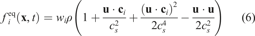
The Boltzmann equation discretized in time, space, and velocity space reads

f_{i} (x + c_{i} Δ t, t + Δ t) = f_{i} (x, t) + Ω_{i} (x, t),

(2)

with Δx as lattice spacing, Δt as time step size and Ω as collision operator. The LB equation can be separated into a collision step

{\tilde{f}}_{i} (x, t) = f_{i} (x, t) + Ω_{i} (x, t)

(3)

and a streaming step

f_{i} (x + c_{i} Δ t, t + Δ t) = {\tilde{f}}_{i} (x, t),

(4)

with

{\tilde{f}}_{i}

denoting the post-collision state of the PDFs.

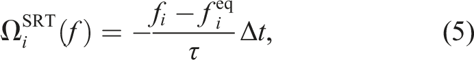
The simplest collision operator is the single relaxation time (SRT) operator

Ω_{i}^{SRT} (f) = - \frac{f_{i} - f_{i}^{eq}}{τ} Δ t,

(5)

which relaxes the PDFs towards the equilibrium f^eq determined by the relaxation time τ. The equilibrium is given by

f_{i}^{eq} (x, t) = w_{i} ρ (1 + \frac{u \cdot c_{i}}{c_{s}^{2}} + \frac{{(u \cdot c_{i})}^{2}}{2 c_{s}^{4}} - \frac{u \cdot u}{2 c_{s}^{2}})

(6)

with the speed of sound

c_{s}^{2} = (1 / 3) Δ x^{2} / Δ t^{2}

and velocity set specific weights w_i. The fluid velocity of a cell at position x is calculated as u (x, t) = ρu (x, t)/ρ(x, t). The kinematic viscosity ν is related to the relaxation time τ and the dimensionless relaxation parameter ω = Δt/τ ∈ ]0,2 [ by

ν = c_{s}^{2} (\frac{τ}{Δ t} - \frac{1}{2}) = c_{s}^{2} (\frac{1}{ω} - \frac{1}{2}) .

(7)

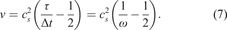
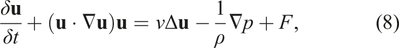
The incompressible Navier-Stokes equation including the kinematic viscosity reads

\frac{δ u}{δ t} + (u \cdot \nabla u) u = ν Δ u - \frac{1}{ρ} \nabla p + F,

(8)

with p as pressure and F as external force term on the fluid.

For a detailed discussion of the theoretical foundations of the LBM and its derivation of the Navier–Stokes equations as the macroscopic limit, see Chen and Doolen (1998) and Krüger et al. (2017).

3. Data structures in waLBerla

In the waLBerla framework, the simulation domain is partitioned into uniform cubic blocks, typically with a size of around 64³ cells on CPUs and about 256³ cells on GPUs. In Figure 1 the block partitioning into uniform cubic blocks is shown. For parts of the domain where no fluid is present, blocks that only consist of obstacle cells can be discarded. The remaining blocks are then distributed to the available MPI processes, so that every process gets at least one block. However, more blocks per process are also possible and can be useful, for example, when load balancing is necessary, as we will see in the following. The organization of a computational grid into blocks introduces a hierarchy that is found essential for efficient processing on the extreme scale since many operations can be better organized in such a hierarchy. In particular, performing the mesh partitioning and load balancing in terms of blocks keeps the complexity and overhead of these algorithms small (see Schornbaum and Rüde (2016) and Schornbaum and Rüde (2018)).

Figure 1.

Exemplary setup of a sparse simulation domain in 2D with a low percentage of fluid covering the domain (light blue), and a high number of obstacle cells. Visualisation of the block partitioning with extraction of blocks without fluid. Illustration of a dense and a sparse data structure for an exemplary setup of 5 × 5 cells per block and a D2Q5 stencil. While the dense data structure stores PDFs and operates on all cells, the sparse data structure only stores and operates on fluid cells.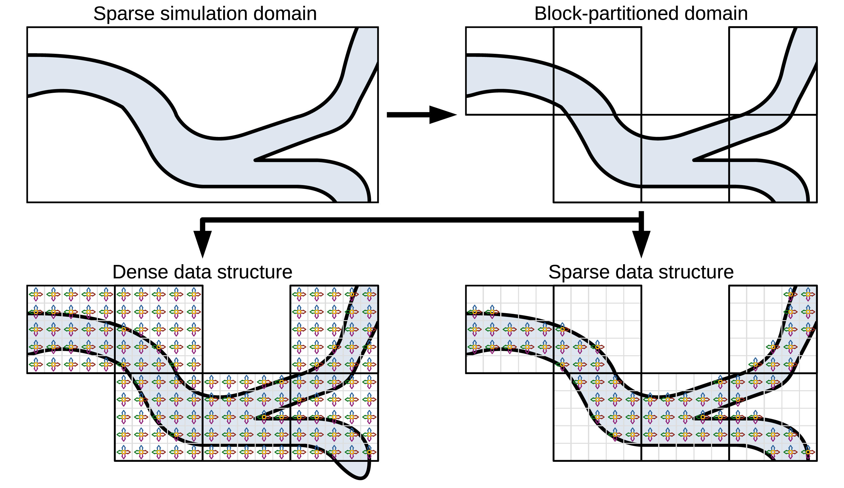

As indicated in Figure 1, the dense/direct-addressing data structure implemented in waLBerla stores the PDFs for every cell in memory, even for non-fluid cells. However, for sparse domains or porous media flows, the porosity

ϕ = \frac{N_{F}}{N}

(9)

with N as the total number of cells and N_F as the number of fluid cells, can be comparatively small. Therefore, much memory may be wasted by storing non-fluid cells on these blocks. Furthermore, a branch statement in the LBM kernel is needed to check, if the current cell is a fluid or an obstacle cell. Additionally, non-fluid cells can cause unnecessary memory traffic, when cache lines contain fluid and non-fluid cells, and hardware prefetchers may read data from non-fluid cells, which is not used. Especially when the domain is sparse, the dense approach creates a significant overhead and can lead to a significant performance loss (Godenschwager et al. (2013)).

3.1. Sparse data structure

To avoid the disadvantages of the dense data structure, we have developed a sparse data structure in waLBerla and lbmpy. Changing the data structure from direct-to indirect-addressing impacts the performance and memory consumption of the LBM solver, but it does not impact the physics of the simulation. As only the representation of the LBM lattice in memory is changed, the physical results stay the same, except negligible deviations caused by potential reordering of the floating point operations.

The idea of the indirect-addressing data structure is to only store fluid cells in a one-dimensional array, we call PDF-list, so that no memory is wasted on storing non-fluid cells. Furthermore, with such a data structure LBM kernels only have to iterate over fluid cells, and no branch conditions are needed in the innermost kernel loops. On the other hand, one loses topological information when storing cell data in a linear array only. With the direct-addressing data structure, PDFs can easily be accessed by their spacial location x and the PDF index i. This access via index arithmetic is not possible for the sparse PDF-list.

A second data structure, the index-list, is introduced to recover the lost spacial information. This list stores the streaming information from one PDF to another. So for one PDF, the index-list stores the location of the PDF, to which it will propagate to in the streaming step. Using the index-list, we can access the neighbors of a cell using one indirection. Therefore, this approach is called an indirect-addressing scheme.

To still have the possibility to access the actual position of the cell x in the domain, another data structure can be stored, that holds the information of the mapping from a cell index to the topological information of the cell. This information is not used in the actual compute kernels, but is useful for postprocessing or the export of simulation data.

While the PDF-list consists of N_F ⋅ Q entries, where Q is the size of the stencil, the index-list only consists of N_F ⋅ (Q − 1) entries, since the center PDF need not to be stored, as no propagation information is needed for the center PDF.

The exact structure of the PDF-list and index-list is illustrated in Figure 2(a) and (b), respectively. We show the PDF-list in a Structure-of-Array (SoA) format, so all PDFs of one direction lie next to each other in memory. The demonstrator domain consists of fluid cells (white), no-slip boundary cells, which indicate an obstacle (grey), velocity bounce back boundary conditions (blue) and ghost layer cells, which are needed for the communication between blocks (light yellow). The index-list is constructed for a pull streaming pattern.

Figure 2.

Structure of the 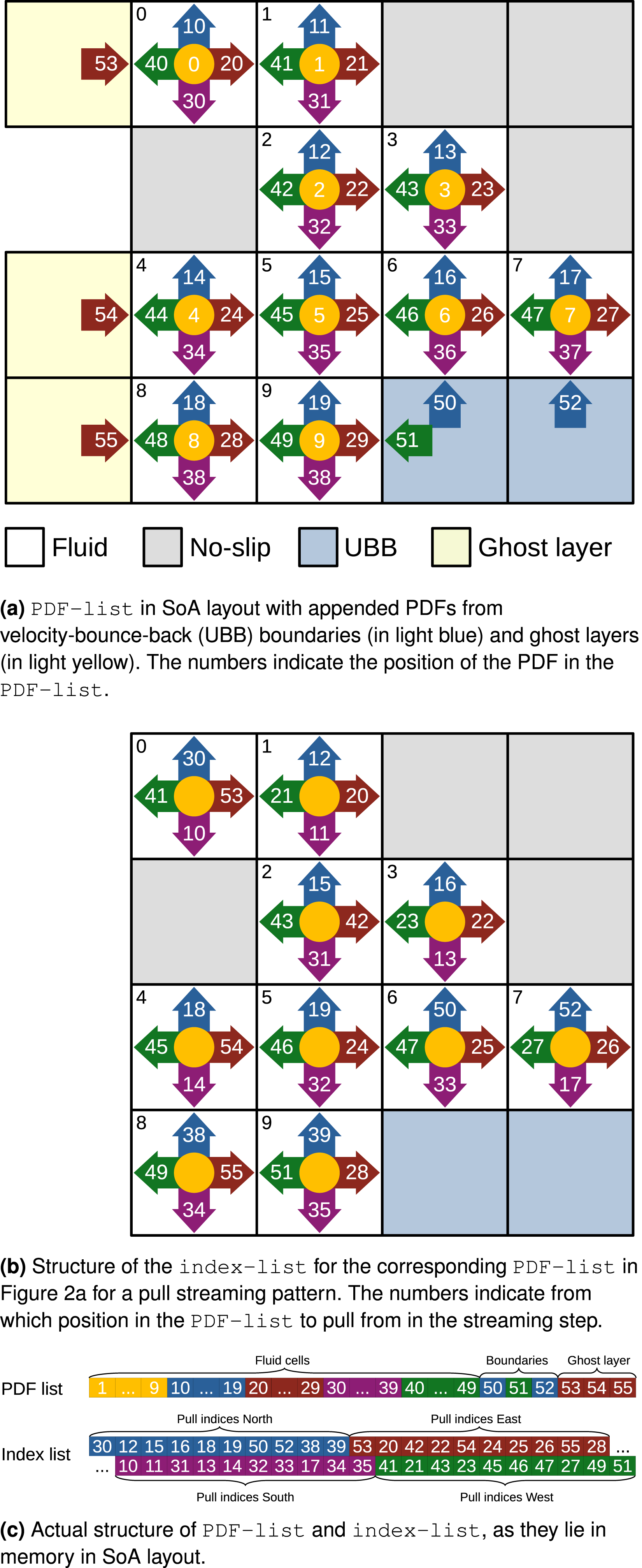PDF-list and the index-list for an exemplary D2Q5 velocity set. The domain contains fluid cells (white), ghost layers (light yellow), velocity-bounce-back (UBB) boundaries (light blue) and no-slip boundaries (grey). The directions of the PDF stencil are indicated by colors as well. In direction west there is a MPI interface to the neighboring block considered. North, east and south cells next to the presented cells are also considered as no-slip cells.

In Figure 2(a) the PDF of cell 0 in direction west $(P D F_{w}^{0})$ is stored at position 40 in the PDF-list, and the $P D F_{w}^{1}$ of cell 1 is stored at position 41. To perform a streaming step for $P D F_{w}^{0}$ in cell 0, we have to look up the pull index (for a presumed pull-streaming pattern) in the index-list. This is illustrated in Figure 2(b), where the pull index of the $P D F_{w}^{0}$ is the PDF 41. This makes sense, as for direction west we pull PDF_w from the right neighbour cell. The pull index look-up in the index-list is done for all PDFs of all fluid cells to perform a complete streaming step. The actual layout of the PDF-list and index-list in memory is illustrated in Figure 2(c). There the SoA layout is used.

As presented in Figure 1, a computational domain is usually split into multiple waLBerla blocks for running a parallelized simulation. Therefore, one PDF-list and one index-list is created per block. These lists hold the PDF and index information for all fluid cells covered by the corresponding block.

3.2. Sparse boundary conditions

Some modifications to the list data structures are made to support the implementation of boundary conditions. No-slip boundary conditions can easily be realised by setting the pull indices of the PDF, which would pull from a no-slip boundary to the inverse direction of the PDF. This is also illustrated in Figure 2(b). For illustration we focus on $P D F_{w}^{1}$ of cell 1. It would pull from its right neighbour cell, but this is an obstacle (no-slip) cell. So $P D F_{w}^{1}$ (PDF 41) pulls from the PDF in east direction of its same cell 1, which is then the $P D F_{e}^{1}$ with index 21. Also, periodic boundary conditions are easy to implement; here, the pull index of the PDF, which must stream from the periodic boundary on the opposite side, is just set to the PDF on the other side of the domain.

For boundary conditions other than no-slip or periodic, PDFs, which correspond to a boundary cell but point to a fluid cell, must be appended to the PDF-list. Further, the index-list has to be modified, so that PDFs of fluid cells next to boundary cells pull from the boundary PDF cells. This is also illustrated for velocity-bounce-back boundary conditions (UBB) in Figure 2. Here, the $P D F_{w}^{9}$ (PDF 49, cell 9, direction west) pulls from PDF_w of the UBB boundary cell right next to it, which is the appended PDF with index 51.

3.3. Sparse communication

For the dense data structure, every block has a ghost layer of at least one cell all around in which it stores the PDFs traveling in the corresponding direction. This ghost layer is used to communicate PDF information between neighboring blocks. For the communication between sparse blocks, we also have to append these ghost layer PDFs to the PDF-list and modify the index-list so that cells next to the MPI interface pull from these ghost layer PDFs, to get valid fluid information from the neighbor block (see Figure 2 yellow cells).

To enable periodic boundary conditions on a domain decomposed into multiple blocks and distributed over multiple MPI processes, the block on the periodic boundary is treated as a neighbor of the block on the opposite side of the domain. Thereby, these blocks communicate PDF information into the ghost layer cells of each other. The cell next to the periodic boundary is then able to pull PDFs from the ghost layer cells of the same block, which correspond to the PDFs of the cell on the opposite side of the periodic domain.

As we only append boundary and ghost-layer PDFs pointing to fluid, the memory overhead of the additionally stored PDFs for handling the boundary conditions and the communication is relatively low. In LBM kernels, we still only need to iterate over fluid cells.

3.4. Code generation for sparse kernels

Many variants of the LBM have been developed over the last decades, which vary in complexity, accuracy, and computational cost. The code generation framework lbmpy is capable to generate kernels for most of these LBMs. To get an overview of lbmpy and the provided functionalities and LBM variants, see Bauer et al. (2021) and Hennig et al. (2022).

For example, the classical collision models such as single-relaxation time (SRT, Qian et al. (1992)), two-relaxation time (TRT, Ginzburg (2005)), and multi-relaxation time (MRT, Dhumieres et al. (2002)) operators are available. However, more advanced collision models are also supported, such as the central moment operator or the cumulant operator. The cumulant LBM, e.g., provides superior accuracy and stability for high Reynolds number flows (see Geier et al. (2015)). The complexity of the collision models increases from the SRT model to the cumulant model in terms of complexity and the number of moment transfers, so e.g. the transfer from moment space to central moment space or to cumulant space. This can increase the number of floating point operations in the collision step significantly. However, due to optimizations such as common sub-expression elimination (CSE), the number of operations per cell lies between only 200 and 400 FLOPS for a D3Q19 stencil irrespective of the collision model (Hennig et al. (2022)). Therefore, the performance of the compute kernels remains memory-bound, as the number of memory accesses stays constant for all collision operators. Consequently, we can report a similar performance for all collision operators in the following in Figure 5.

To profit from the functionalities of the code generation pipeline lbmpy, we integrated the generation of new sparse LBM kernels, boundary handling kernels, and communication kernels. The main difference of the code generation for sparse kernels is the iteration loop and the indexing. In dense kernels, the loop iterates over all cells in a three dimensional way. The sparse kernels, on the other side, only iterate over the one dimensional PDF-list. Further, in dense kernels, the indexing of cells is handled by the position of the cells in the domain. So when a cell with position x needs PDF information from its right neighbor, it will pull from the cell with position x_x+1. In sparse kernels, the indexing of the PDF-list in the streaming step is handled by the index-list.

To save memory accesses, the code generation usually generates a fused stream-collide step, so every PDF has to be loaded and stored only once per time step.

All together, lbmpy is now able to generate efficient sparse kernels for various velocity sets and collision operators, which can run on all common CPUs and NVIDIA and AMD GPUs.

3.4.1. Single node performance

In Figure 3, we present the performance of the generated sparse LBM kernel in comparison to the generated direct-addressing kernel. The diagram shows the mega fluid lattice updates per second (MFLUPs) depending on the porosity ϕ as defined in equation (9). The LB method uses a D3Q19 velocity set and the SRT collision operator. The benchmark measures the LBM kernel performance without boundary handling or communication, and it is performed on a single NVIDIA A100 GPU.

Figure 3.

Single GPU benchmark for sparse, dense and hybrid data structure with varying porosity on a NVIDIA A100 with 256³ cells, D3Q19 velocity set and SRT collision operator. The theoretical performance is calculated from the bandwidth of a streaming benchmark (1361 GB/s) and the theoretical number of memory accesses of the kernels, as LBM code is usually memory bound.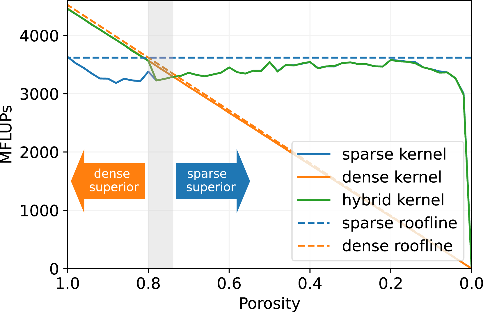

We observe that the single GPU performance of the sparse and the dense kernel is quite close to the theoretical peak performance. As the pure LBM stream-collide step is commonly limited by the memory bandwidth of the architecture, the performance of an efficient LBM kernel should be close to the theoretical peak performance, which is calculated from the memory bandwidth divided by the number of memory accesses needed for updating one LBM cell. This means that the presented kernels sufficiently saturate the memory bandwidth of the NVIDIA A100 GPU. Efficient LBM implementations with a performance close to bandwidth peak are also reported in Zacharoudiou et al. (2023-01), Lehmann et al. (2022) and Wittmann et al. (2013).

Furthermore, Figure 3 shows, that the MFLUPs performance for the sparse kernel remains essentially constant for decreasing porosity. However, we also observe, that the sparse kernel performs worse for ϕ ≥ 0.75. This is caused by the extra memory accesses of the sparse data structure. A dense kernel has to read and write every PDF of a cell per time step. This results in a memory access volume of 2Q ⋅ B_PDF bytes per cell on GPUs, with Q as stencil size, here 19, and B_PDF as the bytes per stored PDF, here 8 bytes for double precision. The sparse kernel, on the other hand, accesses 2Q ⋅ B_PDF + (Q − 1) ⋅ B_idx bytes per cell, because it needs to read neighboring information from the index-list. B_idx is the number of bytes per index in the index-list, here 4 bytes for an integer.

Nevertheless, the performance for the dense kernel decreases linearly when porosity decreases. The reason for this behavior is that dense kernels in waLBerla traverse all cells, including the non-fluid cells. This avoids the need for a branch instruction for non-fluid cells, as mentioned before. On the other side, this leads to a linear decrease of the fluid lattice updates per second.

As indicated in Figure 3, the theoretical break-even point for sparse and dense kernels is approximately ϕ ∼ 0.75.

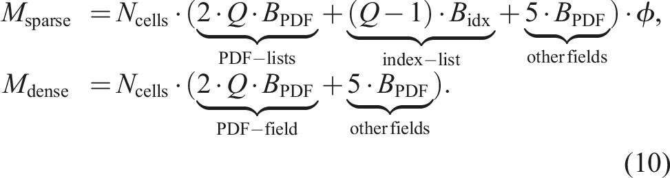
On the same NVIDIA A100 GPU we present a comparison of the memory consumption for a lattice of 256³ cells in Figure 4. The memory usage is measured with the NVIDIA monitoring tool nvidia-smi, showing that the sparse data structure consumes linearly less memory with decreasing porosity. On the other hand, the dense data structure exhibits a constant memory footprint because it stores all cells in the domain, regardless of whether a cell is fluid or boundary. For a porosity of 1.0, where all cells in the domain are fluid, the sparse data structure consumes more memory, since it also has to store the index-list in addition to the PDF-list. The theoretical memory consumption of the LBM kernels can be calculated as:

\begin{align} M_{sparse} & = N_{cells} \cdot (\underset{PDF - lists}{\underset{⏟}{2 \cdot Q \cdot B_{PDF}}} + \underset{index - list}{\underset{⏟}{(Q - 1) \cdot B_{idx}}} + \underset{other fields}{\underset{⏟}{5 \cdot B_{PDF}}}) \cdot ϕ, \\ M_{dense} & = N_{cells} \cdot (\underset{PDF - field}{\underset{⏟}{2 \cdot Q \cdot B_{PDF}}} + \underset{other fields}{\underset{⏟}{5 \cdot B_{PDF}}}) . \end{align}

(10)

Figure 4.

Memory consumption benchmark for 256³ cells on a single NVIDIA A100 GPU for D3Q19 stencil and pull streaming pattern. The theoretical memory consumption is calculated in equation (10).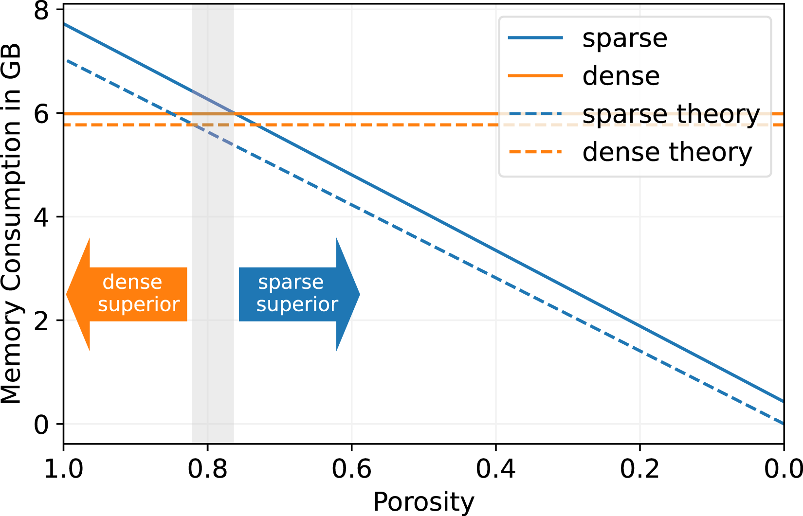

The additional fields stored are a velocity field (3D), a density field (1D), and a flag field to indicate boundary cells (1D).

We see that for the theoretical as well as for the measured memory footprint, the break-even point of the sparse and dense data structure is at a porosity of around ϕ ∼ 0.8, which is a similar result as for the performance comparison. For a higher porosity, the dense data structure is more suitable in terms of memory consumption, and for a lower porosity, the sparse structure becomes superior.

The measured memory consumption for the sparse as well as for the dense LBM in Figure 4 is close to the theoretical memory consumption, so that there is only a small overhead of less than 10% coming from other data structures than the necessary pure PDF data.

3.5. Hybrid data structure

In certain application scenarios, a hybrid data structure may be advantageous. As an example, consider a free flow over a particle bed as depicted in Figure 11. After the domain partitioning, some blocks contain only fluid cells, while other blocks consist primarily of non-fluid cells. In this case, neither the sparse nor the dense data structure seems to fit the given scenario perfectly.

Therefore, we implement the hybrid simulations in waLBerla. From lbmpy, sparse and dense LBM and boundary kernels are generated. In waLBerla, the porosity ϕ is calculated individually on each block to determine the block as a sparse or dense block, based on a porosity threshold ϕ_S. Based on the results in Figures 3 and 4, the porosity threshold should be around ϕ_s ∼ 0.8. During the creation of the data structures on the blocks, a dense PDF field or a sparse PDF-list and the corresponding index-list is created on the block, and only the corresponding generated sparse or dense kernel runs on the blocks. Besides this functionality, appropriate routines for the communication between sparse and dense blocks must be realized. Again, suitable pack and unpack kernels are generated for CPU or GPU architectures with lbmpy, while the MPI communication routine itself stays unchanged.

In Figure 3, we display the performance for the hybrid data structure in green with ϕ_S = 0.8. As expected, the performance reflects that of the dense kernel for ϕ ≥ ϕ_S and, that of the sparse kernel for ϕ < ϕ_S. Consequently, the hybrid approach can always reach the maximum possible waLBerla performance per block, independent of the porosity. The same holds for the memory consumption. If we set the porosity threshold to $\sim 0.8$ as suggested in Figure 4, we also get the best possible memory consumption per block by utilizing the hybrid data structure.

To our knowledge, the presented hybrid approach is a novelty for LBM frameworks, and can be very beneficial for increasing performance and reducing the memory consumption of an application. These benefits depend heavily on the sparsity of the domain.

4. Optimizations to sparse LBM

The high-performance framework waLBerla in combination with lbmpy already provides a wide range of optimizations for LB methods. For the sparse data structure, some of the optimizations had to be adapted or re-implemented. In the following, we specifically describe the effect of implementing an in-place streaming pattern and a communication hiding technique specially designed for the sparse data structures.

4.1. In-place streaming: AA pattern

The most common streaming patterns for LBM are the two-grid algorithms, where either PDFs of a cell are pushed into the neighbor cells (push scheme), or PDFs are pulled from the neighbor cells (pull scheme) (Wellein et al. (2006)). These algorithms have in common that a temporary PDF field is needed. This is because PDFs are stored in a different position than where they are read from. These two-grid streaming patterns read from PDF field A, then they propagate (push/pull) the PDFs, and, lastly, they store the propagated results at a different location in the temporary PDF field B. Therefore, these streaming methods are also called AB patterns. After the propagation, a field swap of fields A and B is needed.

The in-place streaming AA pattern on the other hand, enables writing and storing PDF values in the same positions of the PDF field, so that PDFs can be read from field A and also be written to field A without creating data dependencies. This saves the memory of the temporary PDF field B. Additionally, it also saves memory accesses. We integrated the AA streaming pattern in the code generation pipeline of lbmpy. For details about the functionality of the AA streaming pattern see Bailey et al. (2009).

The benefit of the AA streaming pattern in terms of memory accesses is shown in Table 1. For the pull pattern in dense kernels, 3Q memory accesses are required. One memory access is needed for the read of field A, one is needed for the write on field B, and the third one is a ”write allocate B″, which occurs if the data of the PDF of field B is not already stored in the CPU cache, and therefore has to be loaded into the cache to be written on. A PDF entry is only used once in a fused stream-collide step, and the whole PDF-list is unlikely to fit completely in the CPU cache for large-scale runs. Therefore, the ”write allocate B″ access is mostly present. This memory access only appears on CPUs, as GPUs do not utilize cache structure like CPUs do, so the amount of memory accesses on GPUs per cell is 2Q. Nevertheless, we want to avoid the third access on CPUs by utilizing an in-place streaming pattern. The data is already in the CPU cache because we read and write on the same PDF positions in the same PDF field. By this, we avoid the cache miss and end up with 2Q memory accesses per cell.

Table 1.

Memory accesses per cell for Pull and AA pattern on CPU with size of PDFs B_pdf = 8 Byte, size of indices in the index-list B_idx = 4 Byte and Q = 19.

Memory accesses CPU
	Dense data	Sparse data
Pull	3Q ⋅ B_pdf	3Q ⋅ B_pdf + (Q − 1) ⋅ B_idx
AA	2Q ⋅ B_pdf	2Q ⋅ B_pdf + (Q − 1)/2 ⋅ B_idx
Reduction (1-AA/Pull)	33.3 %	35.6 %

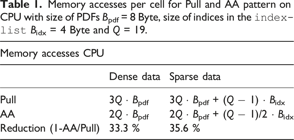
For sparse kernels, utilizing the AA pattern has even more advantages in terms of memory access. For the pull pattern, in addition to the PDF-list, also the index-list has to be read to get the pull accesses for the propagation step, which adds a (Q − 1) to our count of memory accesses. In total, we need 3 ⋅ Q + (Q − 1) memory accesses for sparse LBM kernels with the pull streaming pattern. For the AA pattern on the other side, we only need neighboring information in every second (odd) time step because on even time steps, we only compute cell-local, and therefore no neighboring information is needed. So, the memory accesses for the index list can be halved to (Q − 1)/2.

Therefore, this results in 2Q + (Q − 1)/2 memory accesses for sparse LBM kernels with the AA streaming pattern. We see in Table 1 that the AA pattern on a CPU reduces the memory accesses compared to the pull pattern by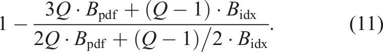

1 - \frac{3 Q \cdot B_{pdf} + (Q - 1) \cdot B_{idx}}{2 Q \cdot B_{pdf} + (Q - 1) / 2 \cdot B_{idx}} .

(11)

Because well-optimized LBM codes are usually memory-bound, an increase in the performance of the LBM by the same ratio can be expected.

As already mentioned above, this performance boost can only be achieved on CPUs, as GPUs do not work with similar caches. No ”write allocate” on the cache can be avoided. Therefore, only half the memory accesses for the index-list can be saved for the sparse approach, as shown in Table 2.

Table 2.

Memory accesses per cell for Pull and AA pattern on GPU with size of PDFs B_pdf = 8 Byte, size of indices in the index-list B_idx = 4 Byte and Q = 19.

Memory accesses GPU
	Dense data	Sparse data
Pull pattern	2Q ⋅ B_pdf	2Q ⋅ B_pdf + (Q − 1) ⋅ B_idx
AA pattern	2Q ⋅ B_pdf	2Q ⋅ B_pdf + (Q − 1)/2 ⋅ B_idx
Reduction (1-AA/Pull)	0 %	9.7 %

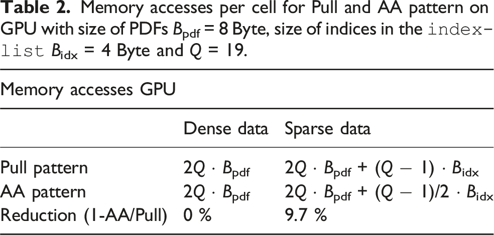
On the other hand, the condition to store the temporary PDF field can be avoided on CPUs and accelerators. So the memory consumption for the sparse LBM in equation (10) shrinks to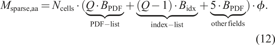

M_{sparse,aa} = N_{cells} \cdot (\underset{PDF - list}{\underset{⏟}{Q \cdot B_{PDF}}} + \underset{index - list}{\underset{⏟}{(Q - 1) \cdot B_{idx}}} + \underset{other fields}{\underset{⏟}{5 \cdot B_{PDF}}}) \cdot ϕ .

(12)

So for a D3Q19 stencil, double precision PDFs, and an integer index-list, we save 36.5% of memory consumption by utilizing the AA streaming pattern for the sparse data structure.

4.1.1. Benchmarking results

In Figure 5 the single GPU benchmarking results for a sparse LBM kernel on a NVIDIA A100 with a D3Q19 stencil and 256³ lattice cells are presented. We compare the pull streaming pattern with the AA pattern for various collision operators. The theoretical peak performance is calculated by the bandwidth, which is 1367 GB/s found by streaming benchmarks (Siefert et al. (2023)), and the number of theoretical memory accesses from Table 2.

Figure 5.

Single GPU Benchmark for pull versus AA streaming pattern for single relaxation time (SRT), two relaxation time (TRT), multi relaxation time (MRT), central moment (CM) and cumulant collision model on a D3Q19 stencil with 256³ cells on a single NVIDIA A100.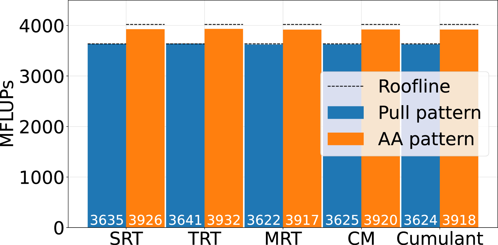

We observe, that the performance of both streaming patterns is close to the theoretical performance for all of the presented collision operators. The average performance increase of the AA pattern compared to the pull pattern on accelerators is $\sim 7.5 %$ , which is close to the theoretically achievable performance increase of 9.7% from Table 2. Therefore, in addition to the avoidance of the storage of the second PDF field, it is also worth to employ the AA pattern on GPUs in terms of performance.

4.2. Communication hiding

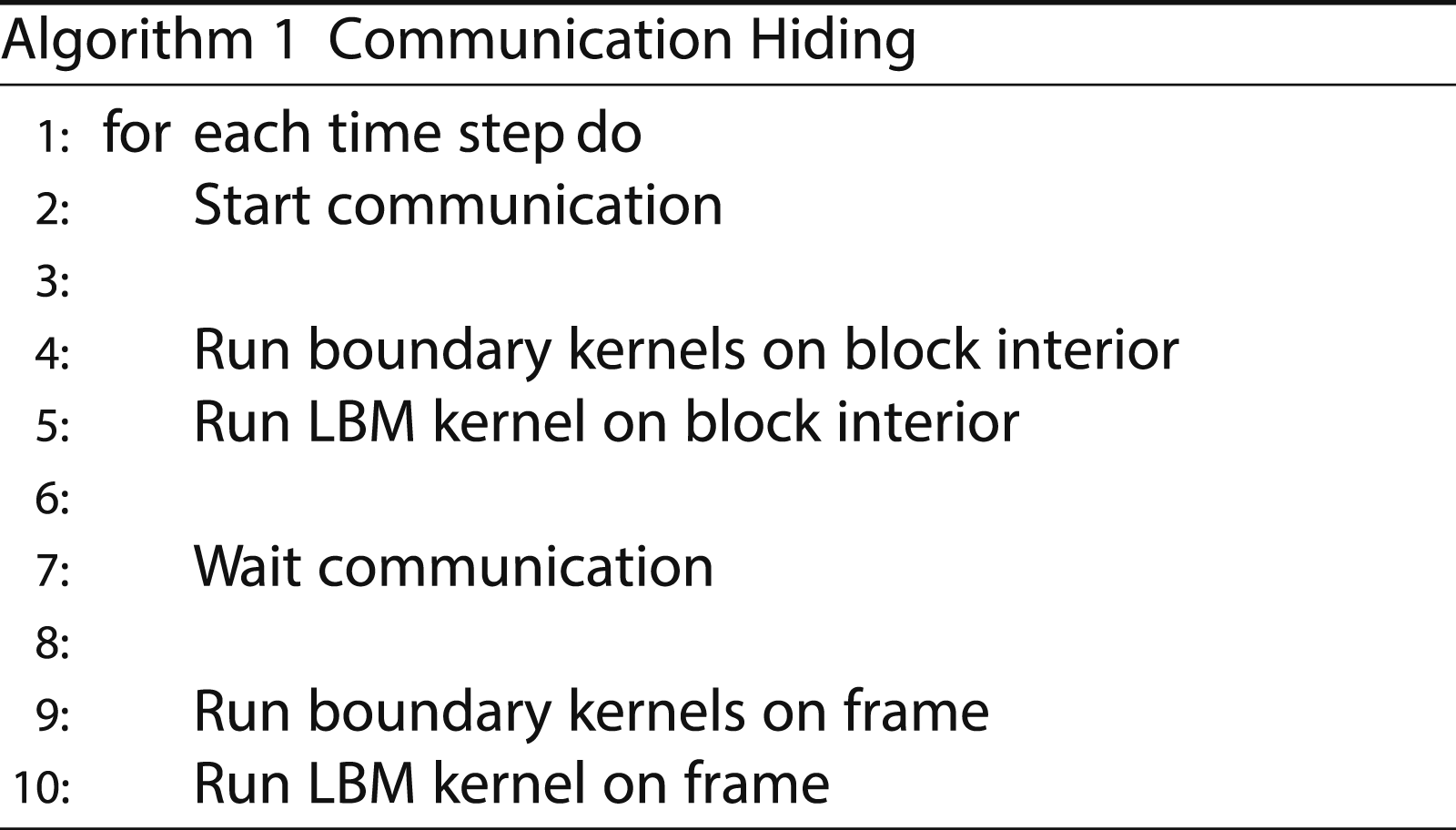
Communication hiding is used to overlap communication with computation. For this, the domain on every block has to be divided into a ”block interior” and a ”frame”, as illustrated in Figure 6. The frame only consists of the outermost cells, while the block interior consists of all other cells. An exemplary code to achieve communication hiding is shown in Algorithm subsection 1. At first, the communication is started. Every block packs its outermost PDFs in an MPI buffer and performs a non-blocking MPI-Send to its neighbors. Now, the block interior cells can be updated because the information from neighbour blocks is not needed for these cells. After this step, the algorithm must wait for the communication to complete and write the information of the MPI buffers to the ghost layers. Lastly, with the updated information in the ghost layers, the LBM and boundary kernels can now be executed on the cells of the frame.

Figure 6.

Subdivision of the PDF field in a frame and the block interior to enable communication hiding. In this example, the frame width is 5 in x, and 3 in y-direction.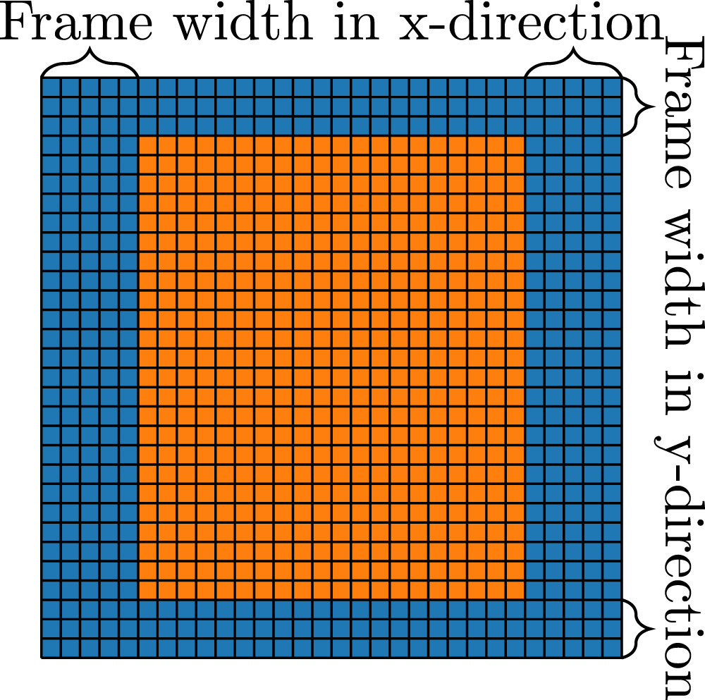

With this algorithm, the communication of the simulation can be overlapped with the kernel on the interior, which leads to higher performance because of better scalability on an increasing number of MPI processes. The width of the frame in all three dimensions has to be chosen suitably to achieve best possible performance. A thinner frame width would increase the number of cells in the interior, providing more time to overlap the communication. On the other hand, a small frame width results in small kernels. Especially on GPUs, small kernels can not fully utilize the GPU, which can lead to performance drops. Additionally, consecutive memory access in one dimension is not possible for a thin frame, which can also reduce the simulation’s performance.

4.2.1. Communication hiding for sparse data structures

Implementing communication hiding for a sparse data structure is not straightforward because there is no topological information for the cells. This means that a cell has no direct information about whether it is inside the block interior or part of the frame. To compensate this, we store two additional index lists, one for the interior and one for the PDFs on the frame. These index lists are initialized by the flag field at the start of the simulation, where spacial information of cells is still present. Furthermore, the pull index for the center PDF of every fluid cell must be stored. This index is used to get the correct write access for kernels on the interior and frame cells. These modifications on the list structure are integrated into the code generation so that they can be turned on and off and allow generated code to run on different architectures.

In the LB framework HemeLB, a comparable communication hiding approach is implemented (Carver et al. (2012); Shealy et al. (2021)).

4.2.2. Scaling results

In Figure 7, the weak scaling of the sparse data structure on the JUWELS Booster HPC cluster is presented. JUWELS Booster is currently place 21 of the Top500 HPC systems (June 2024) and consists of 936 compute nodes, each equipped with 4 NVIDIA A100 GPUs (see Alvarez (2021)).

Figure 7.

Weak scaling benchmark on NVIDIA A100 GPU cluster JUWELS Booster with different configurations for the communication hiding. The roofline is obtained by a stream benchmark (Siefert et al. (2023)). The runs are executed with 320³ cells per GPU, with a D3Q19 stencil and SRT collision model on an empty channel setup.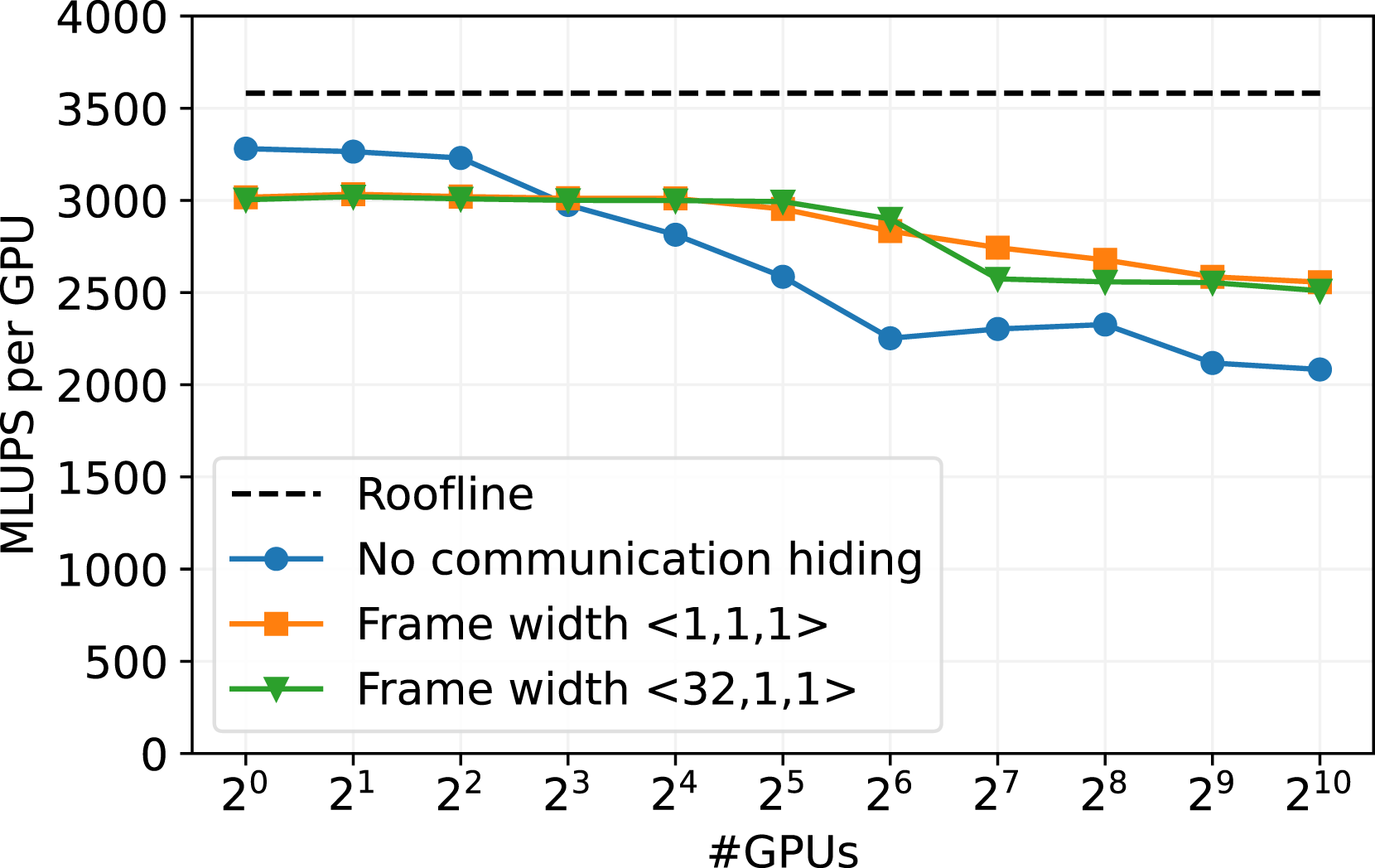

We tested three versions of the communication. One is without communication hiding, one with the minimum frame size of one cell in every direction, and one with a frame thickness of 32 cells in x direction and one cell in y and z direction. This option is promising, since consecutive memory accesses are still enabled in x-direction, while the frame size is still small enough to allow a good communication overlap. In general, a smaller frame size increases the work of the kernels on the interior cells and, therefore, should increase the effectiveness of the communication hiding. On the other hand, the GPU utilization of the kernels on the frame is quite low for a small frame size, and consecutive memory accesses are not secured.

The version without communication hiding performs best up to one node (4 GPUs), see Figure 7. There the intra-node communication speed is quite high since we can exploit the high bandwidth of NVIDIA GPU-to-GPU connections. However, the performance without communication deteriorates for more than 4 GPUs when the inter-node communication speed becomes relevent.

The benchmark runs with communication hiding start with worse performance on single node, as the overhead of the kernel call on the frame cells limits the performance. Nevertheless, these versions exhibit excellent scalability for up to 32 GPUs. Beyond 32 GPUs, the performance drops to 83% scaling efficiency on 1024 GPUs. This can possibly be explained by the InfiniBand network architecture of JUWELS Booster, which is implemented as a DragonFly + network. The drop in performance could be caused by the need for communication between different switch islands of the system when more than 32 GPUs are employed.

In these cases, the size of the frame only has a negligible impact. The two scenarios for communication hiding behave similarly. The smaller frame size of $< 1,1,1 >$ performs a bit better on more than 128 GPUs. Nevertheless, we see that communication hiding can increase the scaling efficiency of the sparse data structure on up to 1024 NVIDIA A100 GPUs from 63% to 83%.

Additionally, we tested the scaling efficiency on the GPU partition of LUMI, which is in the top 5 on the current Top500 list (June 2024). The HPC cluster comprises 2978 nodes with 4 AMDMI250X GPUs per node. Further, every AMD MI250X GPU consists of two Graphical Compute Dices (GCDs) (Pearson (2023)), so we create one MPI process per GCD and show the scaling over the GDCs. As already studied in Holzer et al. (2024), Lehmann (2022) and Martin et al. (2023), it seems not to be possible to achieve significantly better performance than equivalent to approximately 50% of memory bandwidth for LBM codes on a single AMDMI250X. We observe the same behavior in Figure 8.

Figure 8.

Weak scaling benchmark on GPU cluster LUMI-G with different configurations for the communication hiding. The roofline is obtained by a stream benchmark (Siefert et al. (2023)). The AMD MI250X GPUs have two compute chips per GPU (GCDs). The runs are executed with 256³ cells per GCD, with a D3Q19 stencil and SRT collision model on an empty channel setup.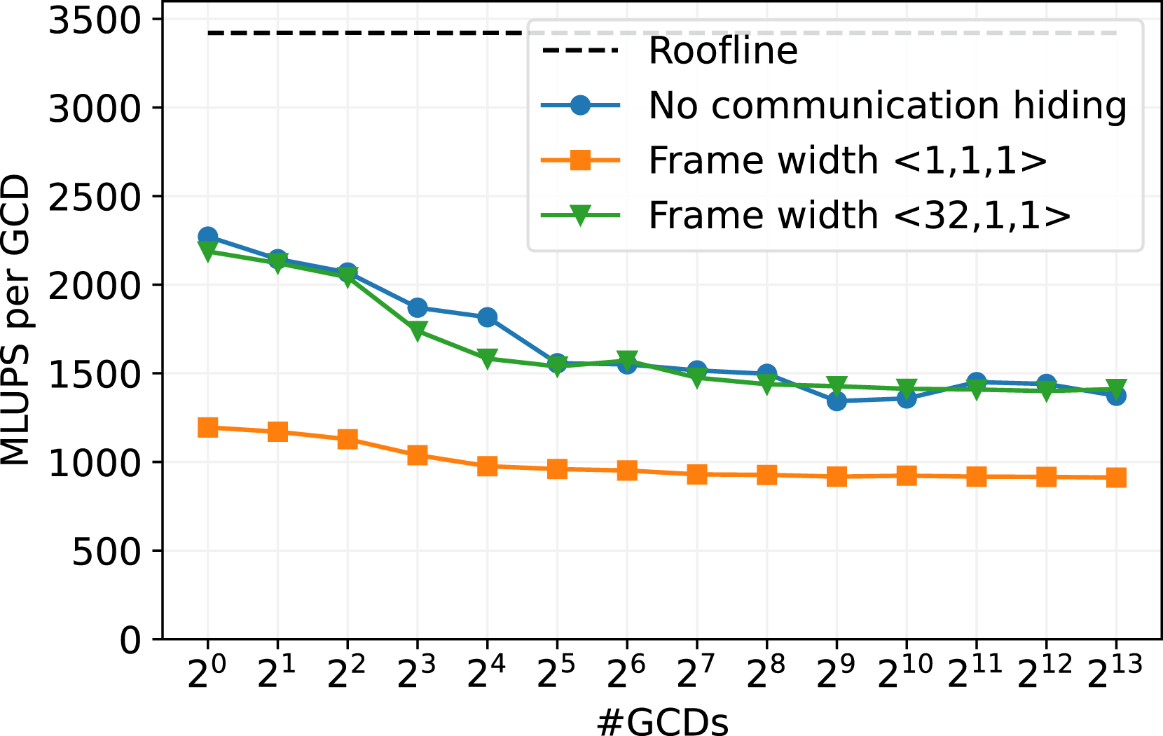

We tested the three communication routines similar to the benchmarks on JUWELS Booster. For the runs without communication hiding, the scaling behavior is similar as for the larger frame size of $< 32,1,1 >$ . For the cases without communication hiding, we achieve a CDG scaling efficiency of 60% scaling from one to 8192 CDGs (4096 GPUs) and a node (4 GPUs) scaling efficiency of 82%. For the greater frame size $< 32,1,1 >$ we observe similar scaling behavior as without communication hiding. The expected acceleration and better scaling could not be observed, a finding that should be further investigated in future research. For the small frame size, the scaling efficiency is almost perfect, but the overall performance is much worse than for the other communication strategies. Again this behavior is unexpected. The non-consecutive memory accesses and kernel calls with small execution times could be the reason for the relatively pour overall performance of the simulation in these cases.

5. Applications

To evaluate the performance of the sparse data structure in a more realistic scenario than the artificial porosity benchmark as in Figure 3 or the weak scaling of an empty channel on JUWELS Booster (Figure 7) and on LUMI (Figure 8), we set up three different applications. The first is a flow through a porous medium consisting of a stationary particle bed. The second one is an extended version of the first application, where the bottom part of the domain consists of the same particle bed, while the upper domain is a free flow, such that we simulate the interaction of a free flow with a porous sediment bed. The last application is the flow through a geometry of coronary arteries, which also results in a complex and sparse domain.

5.1. Flow through porous media

The efficient simulation of fluid flow through porous media is an ongoing research topic, for example in Pan et al. (2004), Yang et al. (2023), Han and Cundall (2013) or Ambekar et al. (2023), to mention a few. For this porous application, we generated a particle bed with the waLBerla molecular dynamics module MESA-PD, as shown in Rettinger and Rüde (2018). We defined a domain of 0.1 m in every dimension and filled it with 21580 particles with a diameter of 0.0041 m. This setup is illustrated in Figure 9 and results in an average porosity of 0.356663.

Figure 9.

Flow through a particle bed consisting of 21580 particles of 0.0041 m diameter, which corresponds to an average porosity of 0.356663. The size of the domain is 0.1 m in every dimension.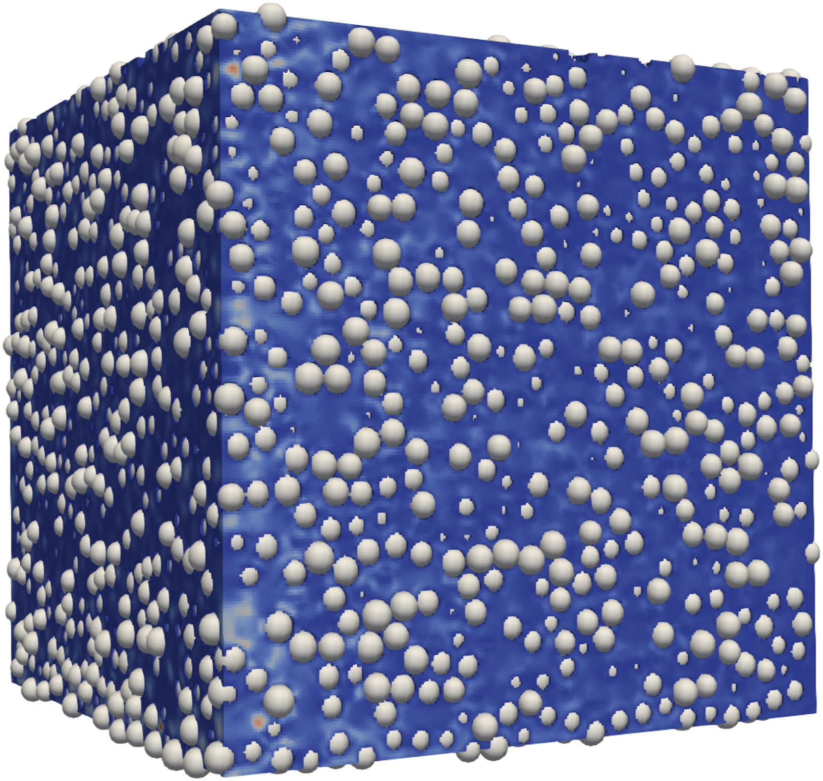

We decomposed the domain with 64 blocks in a 4 × 4 × 4 arrangement to run on 64 NVIDIA A100 GPUs on JUWELS Booster. While we fixed the number of blocks to 64, we increase the cells per block and therefore also the resolution of the domain and the number of total cells, as shown in Figure 10. We performed this benchmark for the sparse data structure, and compare it to the dense data structure.

Figure 10.

Comparison of the sparse and the dense data structure for the flow through the particle bed in Figure 9. The number of 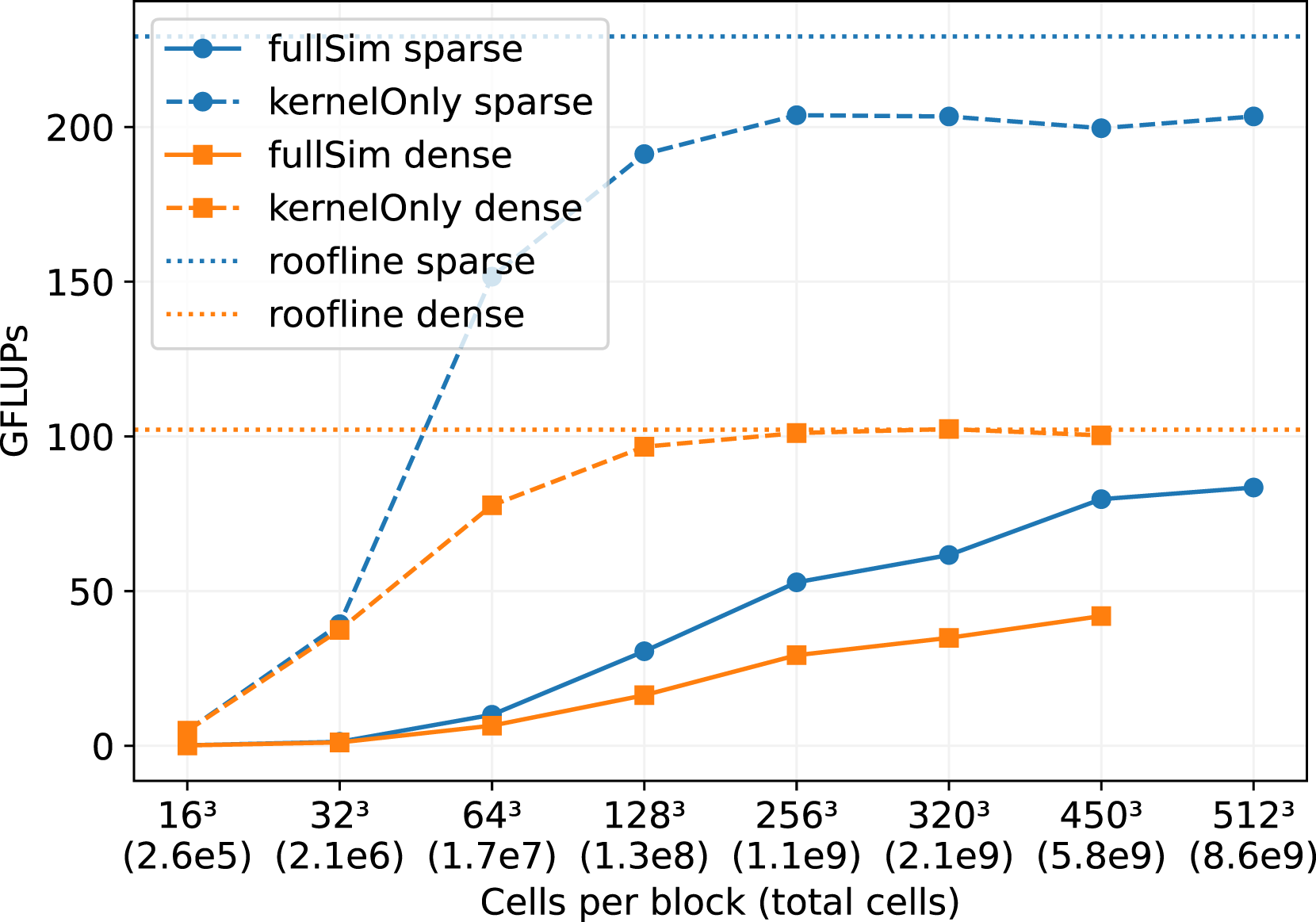waLBerla blocks is fixed to 64 while the cells per blocks increases, and therefore also the resolution and the number of total cells increases. The benchmark was executed on 64 NVIDIA A100 GPUs on JUWELS Booster with one block per GPU.

5.1.1. Kernel-only performance

We first focus on at the ”kernel-only” results in Figure 10, which only show the LBM kernel performance without handling boundaries or performing communication. These results give good insights in the raw performance improvements that we achieved by implementing the sparse data structure, because the performance of the full simulation may be dominated by communication or boundary handling routines. We observe, that for block sizes below 64³, the GPU utilization is too low to achieve good performance. Both, the sparse and the dense kernel saturate at a block size of 256³. Further, we note that the performance of the sparse data structure is approximately two times higher than for the dense structure. This also fits quite well to the results in Figure 3 for a porosity of ϕ ∼ 0.35. The sparse kernel-only performance does not quite reach the theoretical bandwidth limit. This could be caused by some in-balances, since the porosity varies between the blocks, from a minimum of 0.337816 to a maximum of 0.392441. This means, that some blocks, and therefore processes, have more workload in terms of cells. We measure the performance at the end of the simulation run, when all processes finished their work, so the performance is determined by the slowest processor. The performance of the dense kernel on the other side is not affected by the porosity differences, and therefore performs exactly the same work on every MPI process and thus does not suffer from load in-balance issues.

5.1.2. Full-simulation performance

When running the full simulation including boundary handling and communication routines, the overall performance shrinks by at least 50% for both data structures compared to the kernel-only performance. For sparse simulations, the boundary handling has only a small effect on the performance, as the boundary conditions for the particles are implicitly handled by the streaming step (see section about sparse boundary handling). So the main factor is the communication of ghost layer cells between the MPI processes. This communication overhead can be optimized, for example by communication hiding as discussed before, but it can not be avoided completely.

For the full-simulation results in Figure 10, we again observe low performance for small block sizes, which can be explained by the low utilization of GPUs. However, this time, there is no saturation for a block size of 256³ because a more extensive block size results in better communication hiding when the ratio between computational work and communication improves in favor of computational work. For the dense structure, it was not possible to perform simulations with a block size of 512³, as the memory consumption exceeded the 40 GB of the GPU RAM of a single A100. For the sparse structure, this is not a problem, as for a porosity of 0.356,663 we save around 50% of memory compared to the dense structure.

For this application, we significantly benefit from the sparse data structure, as it achieves a performance increase of $\sim 90 %$ compared to the dense one for a block size of 450³. For a block size of 512³, which results in a cell resolution of 4.8828∗10⁻⁵m and 8.6∗10⁹ total cells, it achieves an overall performance of 203.408 GFLUPs for the kernel-only call and 83.475 GFLUPs for the full-simulation run. Further, as shown in Figure 4, for a domain with an average porosity of $\sim 0.35$ , we are able to save around 50% of memory consumption by utilizing the sparse data structure.

5.3. Free flow over river bed

The second application is the simulation of a free flow over a river bed similar to Kemmler et al. (2023) or Fattahi et al. (2016). In Figure 11, the bottom part of the domain consists of the same porous medium/particle bed as the first application in Figure 9, with the same average porosity of about $\sim 0.35$ . The upper part of the domain is a free flow only, so 100% fluid cells in this part of the domain. The average porosity of the domain is $\sim 0.68$ .

Figure 11.

Free Flow over a particle bed. The porosity of the blocks in the particle bed on the bottom (blue blocks) have a porosity of about 0.35, while the upper blocks (red blocks) consists of fluid cells only.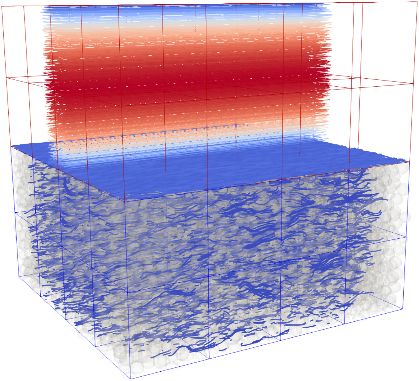

This application is suitable for utilizing the hybrid data structure. As already indicated in Figure 11, the blocks in the upper part of the domain should hold their data in a dense structure (red blocks). In contrast, the blocks in the porous part of the domain should be stored with a sparse data structure (blue blocks). The framework includes the functionality to select the appropriate data structure for each block, the user only has to specify an appropriate porosity threshold.

In Figure 12, a comparison of the sparse, the dense and the hybrid data structure is shown. The simulations are again executed on the JUWELS Booster GPU cluster, with a fixed number of NVIDIA A100 GPUs and one MPI process per GPU. The performance of the raw LBM kernel (kernel-only) is plotted, as well as the entire simulation run, including communication between the MPI processes. We fixed the number of GPUs to 64 as well as the problem size to 10⁹ cells and only vary the cells per block, resulting in a high number of blocks for small cells per block and one block per GPU for the largest block size of 256³ cells.

Figure 12.

Comparison of the sparse, dense and hybrid data structure for the free flow over a particle bed in Figure 11 on 64 NVIDIA A100 GPUs on Juwels Booster. The problem size is fixed to 1.07∗10⁹ cells, while the number of cells per block and therefore also the number of blocks vary. The LBM kernel-only performance is shown as well as the performance of the whole simulation including boundary handling and communication between MPI processes.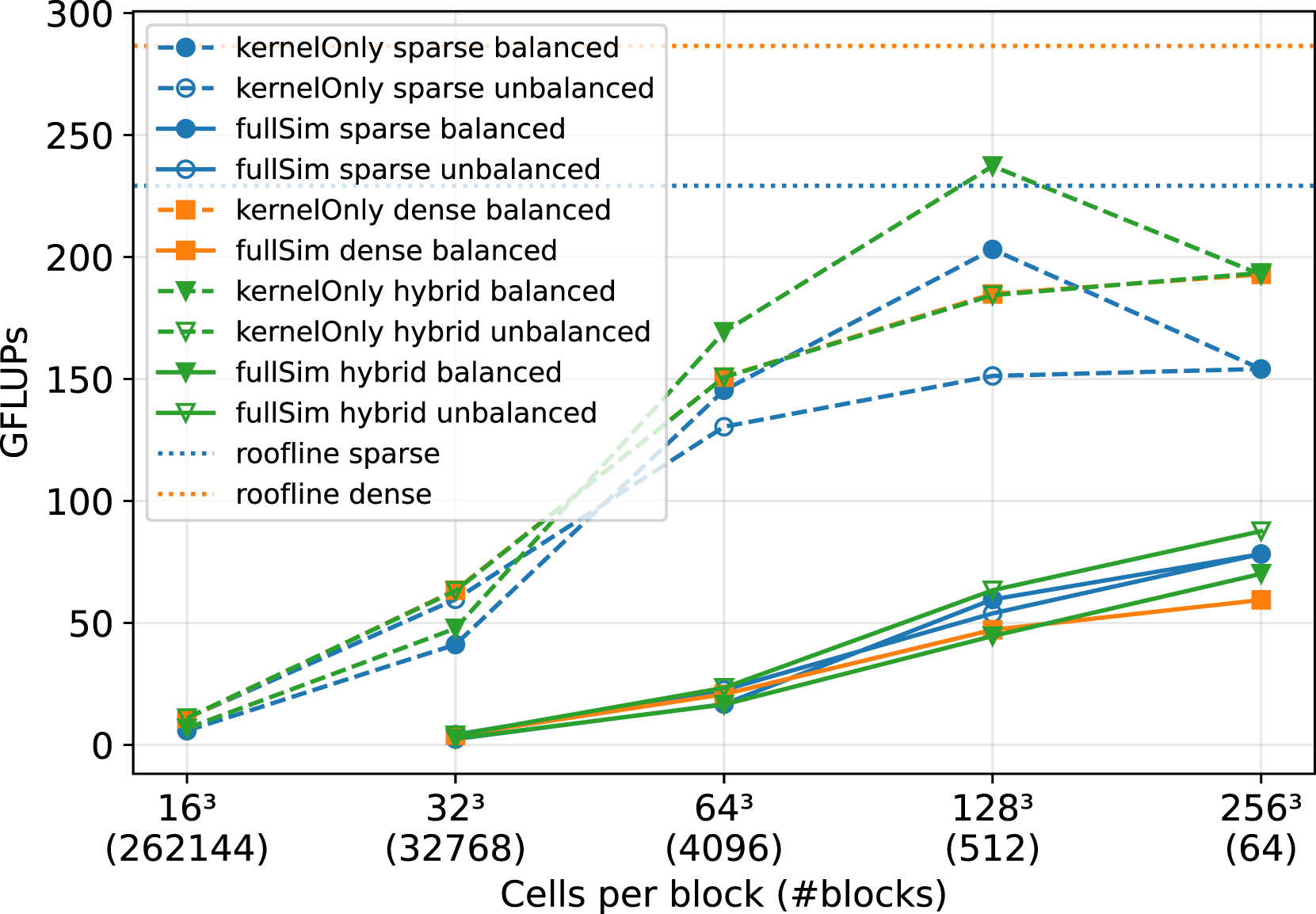

Evaluating the raw kernel performance first, we again observe that a more significant number of cells per block leads to a better utilization of the GPU.

Load-balancing issues can emerge when using a sparse or a hybrid data structure with multiple blocks per GPU. This is because the block partitioning of a domain can lead to a wide span of porosity values on the blocks. When decomposing the river bed simulation in Figure 11 with sparse blocks only, this results in half of the blocks yielding a porosity of 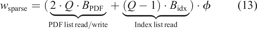$\sim 0.35$ and the other half yielding a porosity of 1.0. One can calculate the workload of a sparse waLBerla block on a GPU similar to the number of memory accesses in Table 2 with

w_{sparse} = (\underset{PDF list read/write}{\underset{⏟}{2 \cdot Q \cdot B_{PDF}}} + \underset{Index list read}{\underset{⏟}{(Q - 1) \cdot B_{idx}}}) \cdot ϕ

(13)

with Q as the stencil size and ϕ as the porosity.

The workload for the dense block on a GPU is

w_{dense} = \underset{PDF field read/write}{\underset{⏟}{2 \cdot Q \cdot B_{PDF}}},

(14)

which is not depending on the porosity of the block.

For the simulation run with sparse data blocks only, the workload of the blocks differs significantly depending on their porosity. Therefore, we employ a load-balancing algorithm to balance the blocks over the MPI processes to reach a better workload distribution. We used a space-filling-Hilbert-curve approach, as described in Schornbaum and Rüde (2018).

5.3.1. Kernel-only performance

In Figure 12, we observe that the load-balancing works well for the sparse kernel-only runs. Especially for the block sizes of 64³ and 128³, the load-balancing seems to reduce the workload unbalance significantly and, therefore, increases the performance. For 256³ cells per block, there is only one block per GPU, so no load-balancing is possible in this case.

No load balancing is necessary for the dense data structure, as every block has the same workload. We see that the kernel-only runs of the dense data structure outperform the unbalanced sparse runs. This is because the sparse data structure is slower than the dense structure on the blocks with a porosity of 1.0 (see again Figure 3), and all MPI processes must wait for the processes holding these blocks. However, when balancing the workload for the sparse kernels, at least for a block size of 128³, we can achieve a higher performance than the dense kernels.

The kernel-only runs for the hybrid data structure without load balancing closely follow the results of the dense kernels in Figure 12. Without load balancing, the low performance of the dense blocks in the porous region heavily dominates the runtime. However, here we can balance the workload to achieve better results. So for the kernel-only runs, using the workload-balanced hybrid data outperforms the other kernels for all block sizes. The only exception is for 256³ cells per block. There no load-balancing is possible, because there is only one block per GPU.

5.3.2. Full-simulation performance

Comparable to the particle bed, the performance of the full-simulation results in Figure 12 is again heavily trimmed by the communication routines, which is not avoidable. For all data structures, the performance increases with increasing block sizes, as the number of blocks and therefore the necessary communication decreases.

Overall, the sparse data structure performs superior to the dense one on the block sizes of 128³ and 256³ cells per block. For the hybrid structure, we observe unexpected behavior. Here, the load-balanced simulation performs worse than the sparse simulations, while the unbalanced hybrid simulation reaches the highest MFLUPs values of all tested data structures. In Table 3, the workload per MPI process of the simulation with the hybrid data structure for 128³ cells per block is presented. We observe that the standard deviation of the average workload is significantly lower than for the unbalanced execution. Still, the performance of the balanced run is worse for the full-simulation. Here we observe that the load-balancing algorithm successfully distributes the workload over the MPI processes but it reduces the spacial locality of the blocks with respect to each other. Therefore, the communication is more expensive.

Table 3.

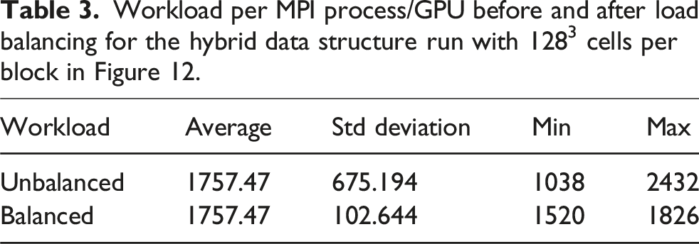
Workload per MPI process/GPU before and after load balancing for the hybrid data structure run with 128³ cells per block in Figure 12.

Workload	Average	Std deviation	Min	Max
Unbalanced	1757.47	675.194	1038	2432
Balanced	1757.47	102.644	1520	1826

Nevertheless, for a complex domain setup such as a free flow over a riverbed, we also manage to improve the application’s performance by utilizing the sparse or the hybrid data structure. Additionally, we note the reduced memory consumption as presented in Figure 4. Overall, when half of the domain consists of a porous medium, such as in Figure 11, we save about 25% of memory with the hybrid data structure.

5.4. Coronary artery

Finally, we present performance results for the flow in a coronary artery. This is a topic of high interest in medical engineering and has been studied, for example, in Axner et al. (2009), Afrouzi et al. (2020), Bernaschi et al. (2010) and Godenschwager et al. (2013). The flow in a coronary artery results in a complex and highly sparse domain. An example setup for this application is shown in Figure 13. While the whole domain would consist of a very high number of blocks, we can discard all blocks that do not contain fluid cells. Still, the remaining blocks have a very low porosity. Of course, when lowering the size of the block, the block structure would converge better to the geometry and result in higher block porosities. However, small block sizes also lead to under-utilization of GPUs, as already shown in Figure 10.

Figure 13.

Domain partitioning of a coronary artery with 1.2 ⋅ 10⁸ fluid cells, 531 blocks and 128³ cells per block.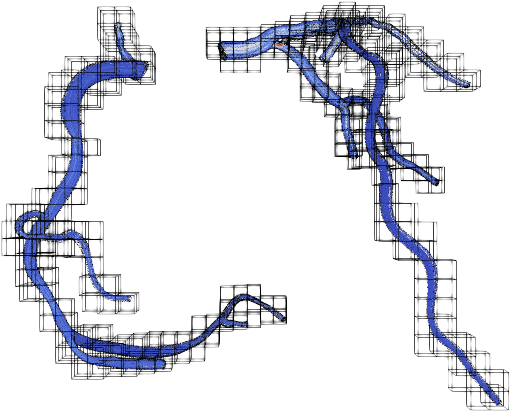

In Figure 14, we compare the performance of the sparse and the dense data structure on JUWELS Booster. We fixed the number of NVIDIA A100 GPUs to 60 and the problem size to 1.2 ⋅ 10⁸ fluid cells while varying the block size and, therefore, also the number of blocks.

Figure 14.

Comparison of the sparse and the dense data structure for the artery flow in Figure 13 on 60 NVIDIA A100 GPUs on JUWELS Booster. The problem size is fixed to a number of 1.2 ⋅ 10⁸ fluid cells, while the block size and therefore also the number of blocks varies.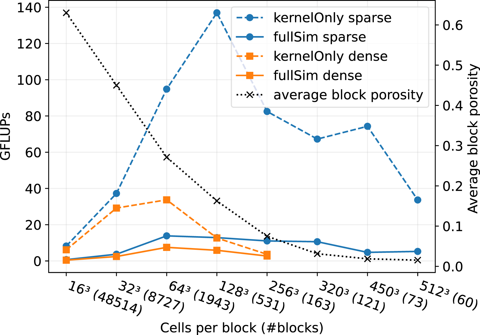

5.5. Kernel-only performance

Again, we observe the behavior of a small block size, which results in low performance for the kernel-only runs of the sparse data structure. We experience that increasing the block size up to 128³ cells per block leads to higher performance of the raw sparse LBM kernel. For block sizes larger than 128³, the porosity drops below ϕ < 0.1. We observe in Figure 3 that the sparse LBM performance starts to deteriorate for a porosity smaller than 0.1. Therefore, for block sizes larger 128³, the performance of the sparse kernel in Figure 14 shrinks because of the low block porosities. The sweet spot between large block sizes for good GPU utilization and a porosity greater than 0.1 for good kernel performance is a block size of 128³ cells per block for this setup.

5.5.1. Full-simulation performance

The performance for the sparse full simulations is relatively stable for moderate block sizes. This is because the performance is heavily dominated by communication, which is especially high in this application because of the high number of blocks per MPI process.

Nevertheless, the sparse data structure shows significantly higher performance than the dense data structure for all block sizes. This is true for the kernel-only runs and the full simulation runs. For a block size of 128³ cells, we achieve a speed-up of about 11 for the kernel-only run and still a speed up of 2 for the full simulation.

5.5.2. Memory consumption

Also remarkable is the amount of memory we can save for the artery setup. So when choosing a block size of 128³ cells per block to reach maximum raw performance; then, we end up with an average block porosity of ϕ ∼ 0.16. This means that according to Figure 4, we save about 75% of memory when using the sparse instead of the dense data structure. We were not able to acquire results for the dense structure for block sizes greater than 256³ because the NVIDIA A100 RAM ran out of memory.

6. Discussion

Parts of this work are comparable to Martin et al. (2023). In this article, the framework HARVEY is ported to different programming models such as CUDA, HIP, SYCL and Kokkos. The authors compare the performance on different hardware, among others also on NVIDIA A100 and AMD MI250X GPUs. HARVEY is a LBM based CFD software with a focus on simulations of blood flow in patient-derived aortas, also utilizing the indirect addressing approach.

Martin et al. (2023) measure the performance of HARVEY and a proxy app for NVIDIA A100 GPUs on the HPC System Polaris³. Their proxy app is used to show the maximum achievable performance for simple test cases. Their results of the proxy app for an empty channel flow on one node (4 NVIDIA A100 GPUs) reaches around 12,000 MLUPS, equivalent to 3000 MLUPS per A100 GPU. This is close to what we achieve, as shown in Figure 7 for the communication-hiding cases. The actual HARVEY framework performs slightly worse for the same empty channel with around 2250 MLUPS per GPU. On the maximum scaling size of 1024 NVIDIA A100 GPUs, the proxy-app reaches around 10⁴ MLUPS, equivalent to 976 MLUPS per GPU. The HARVEY framework achieves around 6∗10⁴ MLUPS, equivalent to 585 MLUPS per A100 GPU. In Figure 7 waLBerla achieves 2500 MLUPS per GPU on 1024 NVIDIA A100 GPUs. We conclude that the scaling efficiency of waLBerla seems to be superior. The results may not be fully comparable, as the team of Martin et al. (2023) performs a piece-wise strong-scaling, while we show the weak scaling of our software. Further, they operated on a different HPC cluster, so especially the scaling performance can depend significantly on the configuration of the HPC system.

When comparing the results for the artery geometry with a resolution of 55 μm, HARVEY achieves around 4∗10⁴ MLUPS for 64 A100 GPUs, so 625 MLUPS per GPU. In Figure 14 waLBerla was able to achieve 1374 MLUPS per GPU for the kernel-only runs, but only 230 MLUPS for the full simulation performance. Of course, the underlying geometry of the artery is different, so again the results may not be fully comparable. Nevertheless, there is still room to optimize the waLBerla framework in terms of load-balancing and communication-efficiency, especially for cases with multiple blocks per GPU.

Further, Martin et al. (2023) show comparable results on the AMD MI250X GPUs, which were tested on the Frontier⁴ HPC system. We compare the results for 4 GCDs. The proxy app of shows around 2250 MLUPS per GCD, while waLBerla shows 2100 MLUPS per GCD (see Figure 8). So also the team of Martin et al. (2023) confirm, that LBM algorithms are not able to achieve more than 60% of the maximum theoretical performance of the AMD MI250X GPUs. For 1024 CDGs, the proxy app shows a performance of around 10⁶ MLUPS, so 976 MLUPS per CDG. waLBerla was able to achieve 1500 MLUPS per GCD on the same number of GCDs, so it shows a slightly better scaling efficiency. Again, the results are not fully comparable, as we compare a weak scaling with a piece-wise strong-scaling and also run on different systems.

Also comparable are the results from Zacharoudiou et al. (2023-01). The authors conducted blood flow simulations with their LBM framework HemeLB on various HPC systems including JUWELS Booster. They were able to achieve a performance of around 200 MLUPS per GPU on the NVIDIA A100 GPUs of JUWELS Booster with a comparable number of cells per GPU $(\sim 1 0^{7})$ and a comparable artery geometry. This performance is quite close to the 230 MLUPS per GPU we achieved for the full simulation run in Figure 14.

7. Conclusion

In this article, we presented the benefit of sparse LBM kernels, especially when using accelerator cards. We presented the integration of the sparse data structure into lbmpy, to be capable of generating efficient compute kernels for various architectures. We compared the sparse and the dense data structure on a single GPU and found that for a domain porosity of $< 0.8$ , the sparse data structure outperforms the dense data structure in terms of performance and memory consumption.

The sparse kernels show excellent performance for the pull streaming pattern for various collision operators such as single-/two-/multi-relaxation times, central moments, or cumulants on a single GPU. We managed to further increase the performance by $\sim 7.5 %$ and reduce the memory consumption by 36.5% by utilizing an AA streaming pattern on GPUs. We were also able to show a scaling efficiency of the sparse data structure of over 82% on the JUWELS Booster and LUMI-G HPC system for 1024 and 4096 GPUs, respectively.

We proposed a novel hybrid data structure, that is able to flexibly switch between the sparse and the dense approach, depending on which subdomains are handled more efficiently with the corresponding data structure.

We set up a porous media flow simulation and achieved a speed-up of 1.9 and reduced the memory consumption by 50%. For an artery blood flow simulation, we gained a speed-up of 2 dependent on the block sizes and achieved a decrease of memory consumption of about 75%. We experienced imbalances in the distribution of the work over the MPI processes when using the sparse data structures. To maximize the efficiency of the sparse LBM, we employed load balancing, but more research is needed to fully optimize the workload distribution while maintaining the spacial locality of the neighboring blocks on neighboring processes.

To further increase the flexibility of the code generation with lbmpy, future work is planned to support the emerging INTEL GPUs by having a SYCL⁵ back-end. As SYCL is available on most currently available systems, the code generation could used to generate optimized sparse LB kernels for all existing and upcoming hardware such as CPU, accelerator cards, or even exotic hardware such as Accelerated Processing Units (APUs) or Field Programmable Gate Arrays (FPGAs).

Footnotes

ORCID iDs

Philipp Suffa

Markus Holzer

Author contributions

P. Suffa: Conceptualization, Methodology, Software, Validation, Formal analysis, Investigation, Data Curation, Writing - Original Draft, Visualization, Project administration. M. Holzer: Conceptualization, Software, Writing - Review & Editing. H. Koestler: Resources, Writing - Review & Editing, Supervision, Funding acquisition. U. Ruede: Writing - Review & Editing, Supervision, Funding acquisition.

Funding

The authors disclosed receipt of the following financial support for the research, authorship, and/or publication of this article: This work was supported by the SCALABLE project (https://www.scalable-hpc.eu/). This project has received funding from the European High-Performance Computing Joint Undertaking (JU) under grant agreement No 956000. The JU receives support from the European Union’s Horizon 2020 research and innovation program and France, Germany, and the Czech Republic. The authors gratefully acknowledge the Gauss Centre for Supercomputing e.V. () for funding this project by providing computing time through the John von Neumann Institute for Computing (NIC) on the GCS Supercomputer JUWELS at Jülich Supercomputing Centre (JSC). We acknowledge the EuroHPC Joint Undertaking for awarding this project access to the EuroHPC supercomputer LUMI, hosted by CSC (Finland) and the LUMI consortium through a EuroHPC Regular Access call. The authors gratefully acknowledge the scientific support and HPC resources provided by the Erlangen National High Performance Computing Center (NHR@FAU) of the Friedrich-AlexanderUniversität Erlangen-Nürnberg (FAU).

Declaration of conflicting interests

The authors declared no potential conflicts of interest with respect to the research, authorship, and/or publication of this article.

Notes

Author biographies

Philipp Suffa is a PhD candidate at FAU. He studied Commputational Engineering and Computer Science at FAU and is one of the core developers of the WALBERLA HPC framework. His research interests focus on CFD with the Lattice Boltzmann Method, turbulent flow applications and software engineering for high performance computing.

Markus Holzer did his PhD at FAU and CERFACS. His Research interests focus on code generation for the Lattice Boltzmann Method and software engineering for high performance computing.

Harald Köstler got his Ph.D. in Computer Science in 2008 on variational models and parallel multigrid Methods in medical image processing. 2014, he finished his habilitation on Efficient Numerical Algorithms and Software Engineering for High-Performance Computing. Currently, he works at the Chair for System Simulation at the FAU. His research interests include software engineering concepts, especially using code generation for simulation software on HPC clusters, multigrid methods, and programming techniques for parallel hardware, especially GPUs. The application areas are computational fluid dynamics, rigid Body dynamics, and medical imaging.

Ulrich Rüde is a retired professor at FAU and is a consultant for CERFACS in Toulouse, France as well as a senior researcher at the Department of Applied Mathematics, VSB-Technical University of Ostrava, Czech Republic. He studied Mathematics and Computer Science at Technische Universität München (TUM) and the Florida State University. He holds a Ph.D. and Habilitation degrees from TUM. His research interest focuses on numerical simulation and high-end computing, particularly computational fluid dynamics, multilevel methods, and software engineering for high-performance computing. He is a Fellow of the Society of Industrial and Applied Mathematics.

References

Afrouzi

Ahmadian

Hosseini

, et al. (2020) Simulation of blood flow in arteries with aneurysm: Lattice boltzmann approach (LBM). Computer Methods and Programs in Biomedicine 187: 105312. https://doi.org/10.1016/j.cmpb.2019.105312

Alvarez

(2021) Juwels cluster and booster: exascale pathfinder with modular supercomputing architecture at juelich supercomputing centre. Journal of large-scale research facilities JLSRF 7: A183. https://doi.org/10.17815/jlsrf-7-183

Ambekar

Schwarzmeier

Rüde

, et al. (2023) Particle-resolved turbulent flow in a packed bed: RANS, LES, and DNS simulations. AIChE Journal 69(1): e17615. https://doi.org/10.1002/aic.17615

Axner

Hoekstra

Jeays

, et al. (2009) Simulations of time harmonic blood flow in the mesenteric artery: comparing finite element and lattice Boltzmann methods. BioMedical Engineering Online 8(1): 23. https://doi.org/10.1186/1475-925X-8-23

Bailey

Myre

Walsh

, et al. (2009) Accelerating lattice boltzmann fluid flow simulations using graphics processors. In: 2009 International Conference on Parallel Processing. IEEE, pp. 550–557. https://doi.org/10.1109/ICPP.2009.38

Bauer

Eibl

Godenschwager

, et al. (2020) Walberla: a block-structured high-performance framework for multiphysics simulations. Computers & Mathematics with Applications 81: 478–501. https://doi.org/10.1016/j.camwa.2020.01.007

Bauer

Köstler

Rüde

(2021) Lbmpy: automatic code generation for efficient parallel lattice Boltzmann methods. Journal of Computational Science 49: 101269. https://doi.org/10.1016/j.jocs.2020.101269

Bernaschi

Succi

Fyta

, et al. (2008) MUPHY: a parallel high performance MUlti PHYsics/Scale code. In: 2008 IEEE International Symposium on Parallel and Distributed Processing. IEEE, pp. 1–8. https://doi.org/10.1109/IPDPS.2008.4536464

Bernaschi

Fatica

Melchionna

, et al. (2010) A flexible high-performance Lattice Boltzmann GPU code for the simulations of fluid flows in complex geometries. Concurrency and Computation: Practice and Experience 22(1): 1–14. https://doi.org/10.1002/cpe.1466

10.

Brodtkorb

Hagen

Sætra

(2013) Graphics processing unit (GPU) programming strategies and trends in GPU computing. Journal of Parallel and Distributed Computing 73(1): 4–13. https://doi.org/10.1016/j.jpdc.2012.04.003

11.

Carver

Groen

Hetherington

, et al. (2012) Coalesced communication: a design pattern for complex parallel scientific. Software. https://doi.org/10.48550/arXiv.1210.4400

12.

Chen

Doolen

(1998) Lattice Boltzmann method for fluid flows. Annual Review of Fluid Mechanics 30(1): 329–364. https://doi.org/10.1146/annurev.fluid.30.1.329

13.

Dhumieres

Ginzburg

Krafczyk

, et al. (2002) Multiple-relaxation-time lattice boltzmann models in 3D. Philosophical Transactions of the Royal Society of London 360: 437–451. https://doi.org/10.1098/rsta.2001.0955

14.

Fattahi

Waluga

Wohlmuth

, et al. (2016) Large scale lattice Boltzmann simulation for the coupling of free and porous media flow. High Performance Computing in Science and Engineering 9611: 1–18. https://doi.org/10.1007/978-3-319-40361-8.1

15.

Geier

Schönherr

Pasquali

, et al. (2015) The cumulant lattice Boltzmann equation in three dimensions: theory and validation. Computers & Mathematics with Applications 70(4): 507–547. https://doi.org/10.1016/j.camwa.2015.05.001

16.

Ginzburg

(2005) Equilibrium-type and link-type lattice Boltzmann models for generic advection and anisotropic-dispersion equation. Advances in Water Resources 28(11): 1171–1195. https://doi.org/10.1016/j.advwatres.2005.03.004

17.

Godenschwager

Schornbaum

Bauer

, et al. (2013) A framework for hybrid parallel flow simulations with a trillion cells in complex geometries, In: Proceedings of the International Conference on High Performance Computing, Networking, Storage and Analysis, SC ’13. New York, NY, USA: Association for Computing Machinery, pp. 1–12. https://doi.org/10.1145/2503210.2503273

18.

Han

Cundall

(2013) LBM–DEM modeling of fluid–solid interaction in porous media. International Journal for Numerical and Analytical Methods in Geomechanics 37(10): 1391–1407. https://doi.org/10.1002/nag.2096

19.

Hasert

Masilamani

Zimny

, et al. (2014) Complex fluid simulations with the parallel tree-based Lattice Boltzmann solver Musubi. Journal of Computational Science 5(5): 784–794. https://doi.org/10.1016/j.jocs.2013.11.001

20.

Hennig

Holzer

Rüde

(2022) Advanced Automatic Code Generation for Multiple Relaxation-Time Lattice Boltzmann Methods. https://doi.org/10.48550/arXiv.2211.02435

21.

Hijma

Heldens

Sclocco

, et al. (2023) Optimization techniques for GPU programming. ACM Computing Surveys 55(11): 239:1–239. https://doi.org/10.1145/3570638

22.

Holzer

Mitchell

Leonardi

, et al. (2024) Development of a central-moment phase-field lattice Boltzmann model for thermocapillary flows: droplet capture and computational performance. Journal of Computational Physics 518: 113337. https://doi.org/10.1016/j.jcp.2024.113337

23.

Januszewski

Kostur

(2014) Sailfish: a flexible multi-gpu implementation of the lattice boltzmann method. Computer Physics Communications 185(9): 2350–2368. https://doi.org/10.1016/j.cpc.2014.04.018

24.

Kemmler

Schwarzmeier

Rettinger

, et al. (2023) Geometrically resolved simulation of upstream migrating antidune Formation and propagation. In: 40th IAHR World Congres. IAHR.

25.

Krause

Kummerländer

Avis

, et al. (2021) OpenLB—Open source lattice Boltzmann. Computers & Mathematics with Applications 81: 258–288. https://doi.org/10.1016/j.camwa.2020.04.033

26.

Krüger

Kusumaatmaja

Kuzmin

, et al. (2017) The Lattice Boltzmann Method. Springer International Publishing. https://doi.org/10.1007/978-3-319-44649-3

27.

Lai

Tian

, et al. (2020) Hybrid MPI and CUDA parallelization for CFD applications on Multi-GPU HPC Clusters. Scientific Programming 2020: e8862123–e88621215. https://doi.org/10.1155/2020/8862123

28.

Latt

Malaspinas

Kontaxakis

, et al. (2021) Palabos: parallel lattice Boltzmann Solver. Computers & Mathematics with Applications 81: 334–350. https://doi.org/10.1016/j.camwa.2020.03.022

29.

Lehmann

(2022) Esoteric pull and esoteric push: two simple In-Place streaming schemes for the lattice boltzmann method on GPUs. Computation 10(6): 92. https://doi.org/10.3390/computation10060092

30.

Lehmann

Krause

Amati

, et al. (2022) On the accuracy and performance of the lattice Boltzmann method with 64-bit, 32-bit and novel 16-bit number formats. Physical Review E 106(1): 015308. https://doi.org/10.1103/PhysRevE.106.015308

31.

Liu

Chu

, et al. (2023) Accelerating large-scale CFD simulations with lattice Boltzmann method on a 40-Million-Core sunway supercomputer. In: Proceedings of the 52nd International Conference on Parallel Processing. Salt Lake City UT USA: ACM, pp. 797–806. https://doi.org/10.1145/3605573.3605605

32.

Martin

Liu

Ladd

, et al. (2023) Performance evaluation of heterogeneous GPU programming frameworks for hemodynamic simulations Proceedings of the SC ’23 Workshops of the International Conference on High Performance Computing, Network, Storage, and Analysis. Denver CO USA: ACM, pp. 1126–1137. https://doi.org/10.1145/3624062.3624188

33.

Mattila

Puurtinen

Hyväluoma

, et al. (2016) A prospect for computing in porous materials research: very large fluid flow simulations. Journal of Computational Science 12: 62–76. https://doi.org/10.1016/j.jocs.2015.11.013

34.

Mazzeo

Coveney

(2008) HemeLB: a high performance parallel lattice-Boltzmann code for large scale fluid flow in complex geometries. Computer Physics Communications 178(12): 894–914. https://doi.org/10.1016/j.cpc.2008.02.013

35.

Pan

Prins

Miller

(2004) A high-performance lattice Boltzmann implementation to model flow in porous media. Computer Physics Communications 158(2): 89–105. https://doi.org/10.1016/j.cpc.2003.12.003

36.

Pearson

(2023) Interconnect Bandwidth Heterogeneity on AMD MI250x and Infinity Fabric. https://doi.org/10.48550/arXiv.2302.14827

37.

Qian

D’Humières

Lallemand

(1992) Lattice BGK models for navier-stokes equation. Europhysics Letters 17(6): 479–484. https://doi.org/10.1209/0295-5075/17/6/001

38.

Rak

(2024) Parallel programming in the hybrid model on the HPC clusters. In: Malhotra

Sumalatha

Yassin

SMW

, et al. (eds) High Performance Computing, Smart Devices and Networks. Singapore: Springer Nature, pp. 207–219. https://doi.org/10.1007/978-981-99-6690-5...15

39.

Randles

Kale

Hammond

, et al. (2013) Performance analysis of the lattice Boltzmann model beyond navier-stokes. In: 2013 IEEE 27th International Symposium on Parallel and Distributed Processing. Cambridge, MA, USA: IEEE, pp. 1063–1074. https://doi.org/10.1109/IPDPS.2013.109

40.

Randles

Draeger

Oppelstrup

, et al. (2015) Massively parallel models of the human circulatory system. In: Proceedings of the International Conference for High Performance Computing, Networking, Storage and Analysis, SC ’15. New York, NY, USA: Association for Computing Machinery, pp. 1–11. https://doi.org/10.1145/2807591.2807676

41.

Rettinger

Rüde

(2018) A coupled lattice Boltzmann method and discrete element method for discrete particle simulations of particulate flows. Computers & Fluids 172: 706–719. https://doi.org/10.1016/j.compfluid.2018.01.023

42.

Schornbaum

Rüde

(2016) Massively parallel algorithms for the lattice boltzmann method on non-uniform grids. SIAM Journal on Scientific Computing 38(2): C96–C126. https://doi.org/10.1137/15M1035240

43.

Schornbaum

Rüde

(2018) Extreme-scale block-structured adaptive mesh refinement. SIAM Journal on Scientific Computing 40(3): C358–C387. https://doi.org/10.1137/17M1128411

44.

Shealy

Yousefi

Srinath

, et al. (2021) GPU acceleration of the HemeLB code for lattice boltzmann simulations in sparse complex geometries. IEEE Access 9: 61224–61236. https://doi.org/10.1109/ACCESS.2021.3073667

45.

Siefert

Pearson

Olivier

, et al. (2023) Latency and bandwidth microbenchmarks of US department of energy systems in the June 2023 top 500 list. In: Proceedings of the SC ’23 Workshops of the International Conference on High Performance Computing, Network, Storage, and Analysis. Denver CO USA: ACM, pp. 1298–1305. https://doi.org/10.1145/3624062.3624203

46.

Spinelli

Horstmann

Masilamani

, et al. (2023) HPC performance study of different collision models using the Lattice Boltzmann solver Musubi. Computers & Fluids 255: 105833. https://doi.org/10.1016/j.compfluid.2023.105833

47.

Vidal

Roy

Bertrand

(2010) On improving the performance of large parallel lattice Boltzmann flow simulations in heterogeneous porous media. Computers & Fluids 39(2): 324–337. https://doi.org/10.1016/j.compfluid.2009.09.011

48.

Wang

Zhang

Bengough

, et al. (2005) Domain-decomposition method for parallel lattice Boltzmann simulation of incompressible flow in porous media. Physical Review E 72(1): 016706. https://doi.org/10.1103/PhysRevE.72.016706

49.

Watanabe

(2022) Performance evaluation of lattice Boltzmann method for fluid simulation on A64FX processor and supercomputer fugaku. In: International Conference on High Performance Computing in Asia-Pacific Region. Virtual Event Japan: ACM, pp. 1–9. https://doi.org/10.1145/3492805.3492811

50.

Wellein

Zeiser

Hager

, et al. (2006) On the single processor performance of simple lattice Boltzmann kernels. Computers & Fluids 35(8-9): 910–919. https://doi.org/10.1016/j.compfluid.2005.02.008

51.

Wittmann

Zeiser

Hager

, et al. (2013) Comparison of different propagation steps for lattice Boltzmann methods. Computers & Mathematics with Applications 65(6): 924–935. https://doi.org/10.1016/j.camwa.2012.05.002

52.

Yang

Chen

, et al. (2023) Implementation of a direct-addressing based lattice Boltzmann GPU solver for multiphase flow in porous media. Computer Physics Communications 291: 108828. https://doi.org/10.1016/j.cpc.2023.108828

53.

Zacharoudiou

McCullough

Coveney

(2023) Development and performance of a HemeLB GPU code for human-scale blood flow simulation. Computer Physics Communications 282: 108548. https://doi.org/10.1016/j.cpc.2022.108548

54.

Zeiser

Hager

Wellein

(2009) Benchmark analysis and application results for lattice boltzmann simulations on NEC SX vector and intel nehalem systems. Parallel Processing Letters 19(04): 491–511. https://doi.org/10.1142/S0129626409000389

Architecture specific generation of large scale lattice Boltzmann methods for sparse complex geometries

Abstract

Keywords

1. Introduction

2. Lattice Boltzmann method

3. Data structures in waLBerla

3.1. Sparse data structure

3.2. Sparse boundary conditions

3.3. Sparse communication

3.4. Code generation for sparse kernels

3.4.1. Single node performance

3.5. Hybrid data structure

4. Optimizations to sparse LBM

4.1. In-place streaming: AA pattern

4.1.1. Benchmarking results

4.2. Communication hiding

4.2.1. Communication hiding for sparse data structures

4.2.2. Scaling results

5. Applications

5.1. Flow through porous media

5.1.1. Kernel-only performance

5.1.2. Full-simulation performance

5.3. Free flow over river bed

5.3.1. Kernel-only performance

5.3.2. Full-simulation performance

5.4. Coronary artery

5.5. Kernel-only performance

5.5.1. Full-simulation performance

5.5.2. Memory consumption

6. Discussion

7. Conclusion

Footnotes

ORCID iDs

Author contributions

Funding

Declaration of conflicting interests

Notes

Author biographies

References