Sage Journals: Discover world-class research

Abstract

The direct solution of batches of band linear systems in parallel is important for many applications. In this paper, we elaborate on three new GPU algorithms for the data-parallel direct solution of linear system batches, sharing a band structure. We develop algorithms for three matrix types: tridiagonal, small bandwidth, and wide bandwidth. We exploit the band structure of the matrix, and store it in an efficient fashion (LAPACK band matrix format) and ensure that the SIMD parallelism of the GPUs are maximized. We develop a panel-based factorization for wide-band matrices to ensure coalesced access (with column-major storage) while minimizing main memory traffic. For the tridiagonal solvers, to ensure a high level of concurrency, we adapt a divide-and-conquer approach and utilize co-operative group functionality to efficiently communicate between compute units (in registers) on GPUs. We implement these algorithms for NVIDIA GPUs and study the performance for varying matrix sizes (16 to 1024) and across a range of batch items (upto 1 × 10⁶). We compare the performance of our implementations with the corresponding optimized vendor implementations (cuSPARSE and MKL), with the state-of-the-art GPU library MAGMA, and with the optimized LAPACK implementation provided by Intel MKL on Intel Skylake CPUs. We also showcase the effectiveness of our batched band solvers for matrices originating from XGC, a gyrokinetic Particle-In-Cell (PIC) application optimized for modeling the edge region plasma within a plasma physics application. We show that our implementations are on average ∼ 2× (for batched banded solvers, compared to MAGMA and MKL) to ∼ 3× (for batched tridiagonal solvers, compared to cuSPARSE) faster than the state-of-the-art and the vendor provided implementations.

Keywords

batched algorithms band linear systems GPU computing direct solvers LU factorization partial pivoting

1. Introduction

Many computational science applications such as plasma physics and combustion simulations use Ordinary Differential Equations (ODEs) for modeling the physics and the chemical processes in a grid of cells covering the simulation domain. The solution of the ODEs for the distinct cells results in many linear systems of small size that all share the same sparsity pattern. Often, the discretization is based on finite difference schemes, based on stencils of varying width. The stencil width on a grid defines the band-structure of the assembled matrix. When multiple independent quantities need to be computed on the same grid, a finite difference discretization leads to the assembled matrices sharing a sparsity pattern (with a band structure). To evolve the physics in space-time (Hindmarsh (2002)), a non-linear solver is required. For robustness and stability, implicit methods are usually preferred, and a linearization step necessitates the solution of a sequence of linear systems.

For applications that need to solve for non-coupled variables such as concentration of chemical species, the linear systems for the distinct cells are independent. Therefore, in each non-linear solve, there is a need for solver functionality that can efficiently handle a large number of (relatively small) independent linear systems. For the efficient solution of these independent linear systems, batched methods have been developed (Dongarra et al. (2016)).

Batched methods are well-suited for the hierarchical parallelism provided by many-core architectures such as GPUs. Mapping the independent linear system solutions to a coarser level enables synchronization-free computing, while the finer level of parallelism can still be utilized to accelerate the solution of the individual linear systems (Nayak (2023)).

Direct solvers for linear systems consist of two steps: A factorization-step such as LU factorization, that factorizes the matrix into upper and lower triangular factors (A = LU), and a solve step, which involves two triangular solves. For numerical stability, partial pivoting is usually necessary (Davis (2006)), which involves exchanging the rows of the matrix to ensure that the diagonal is not close to zero. Band matrices have a uniform sparsity pattern. We can therefore use a special storage format (based on LAPACK (Blackford and Dongarra (1991))), with only minimal additional storage required for fill-in due to partial pivoting.

With GPUs providing most of the computing power in the latest supercomputers, it is important to deploy algorithms that harness the massive parallelism provided by these architectures. Maximizing performance on the GPU can be challenging due to its massive fine-grained level of parallelism. Batched methods can take advantage of this massive fine-grained parallelism due to their embarrassingly parallel nature, but ensuring efficient mapping of data to the GPU is still challenging. Efficient solution of batched band matrices requires the implementation to ensure that within the fine-grained level, parallel workers have a balanced workload. Additionally, maximizing the cache utilization with efficient storage formats and access patterns for different sub-classes of band matrices (narrow bands, wide bands, tridiagonal etc.) is non-trivial (Abdelfattah et al. (2023)).

In this paper, we showcase our batched band solver algorithms, and their high performance implementations for arbitrary band sizes, and specializations for wide bands and tridiagonal matrices. The novel contributions of this paper are listed below:

(1) General batched band matrix solver algorithms for GPUs that outperform existing state-of-the-art CPU and GPU solvers, with a column-based LU factorization and fused triangular solves.

(2) A new variant of a blocked band solver algorithm that enables the efficient solution for wide bandwidth matrices, with adaptable panel sizes to maximize cache utilization and enable coalesced memory accesses.

(3) A batched tridiagonal solver algorithm that outperforms the vendor libraries, using a divide-and-conquer approach to maximize concurrency.

(4) A detailed performance evaluation of the GPU band solvers for randomly generated matrices and an analysis investigating the performance impact of partial pivoting. Additionally, we consider matrices originating from a plasma physics application, XGC, to showcase the performance of our batched band solver in real-world applications.

In Section 2, we provide a background of band matrices, their storage formats and on direct solvers, including their relevance in scientific computing applications. We consider some related work in Section 3. In Section 4, we provide details of our band and tridiagonal solver algorithms, including implementation and optimization details that enable efficient computation on GPUs. We evaluate the performance of our band solvers and benchmark them against state-of-the-art band solvers in Section 5. We conclude with a brief summary in Section 6.

2. Background

Direct methods for the solution of linear systems compute the solution via a fixed and pre-defined sequence of operations. Direct solvers typically factorize the coefficient matrix in the first step and then solve the linear system with forward and backward substitutions. For a general matrix of size n, the factorization step has a computational cost of $O (n^{3})$ , which makes the approach expensive and thus unattractive for large problems. Iterative methods that compute a sequence of solution approximations with increasing accuracy are thus often preferred. These methods have a complexity of $O (k \cdot n n z)$ (where nnz is the number of nonzeros, and k is the number of iterative steps performed), which for large sparse problems is cheaper than $O (n^{3})$ . However, direct solvers are still attractive if the linear system is of small size, ill-conditioned, or if the factorized matrix can be re-used (e.g. when solving with multiple right hand sides). The most common general direct solver is the LU factorization combined with the triangular solves (Duff et al. (2017)).

Algorithms for the factorization and subsequent solution can account for the sparsity pattern and symmetry of the matrix. While for small matrices, using a dense storage format is acceptable, storing large matrices in the dense format can be inefficient or even impossible if the memory requirements exceed the hardware resources. Efficient algorithms have been developed for these cases that handle the coefficient matrix and the factorization in sparse matrix formats such as CSR (Duff et al. (2017); Li and Demmel (2003)). When using sparse data formats, the factorization step is typically split into two stages, a symbolic phase where the row dependencies and fill-in are determined, and a numeric phase where the actual factorization and the numeric values are computed.

The sparsity pattern of the generated matrix depends on the application. Many applications require the solution of linear systems whose matrices have a band structure, for example, those that arise from a stencil discretization. Band matrices are characterized by two main parameters: the lower bandwidth, β_L, and the upper bandwidth, β_U, as shown in Figure 1 with (β_L, β_U) = (3, 1).

Figure 1.

Band matrix 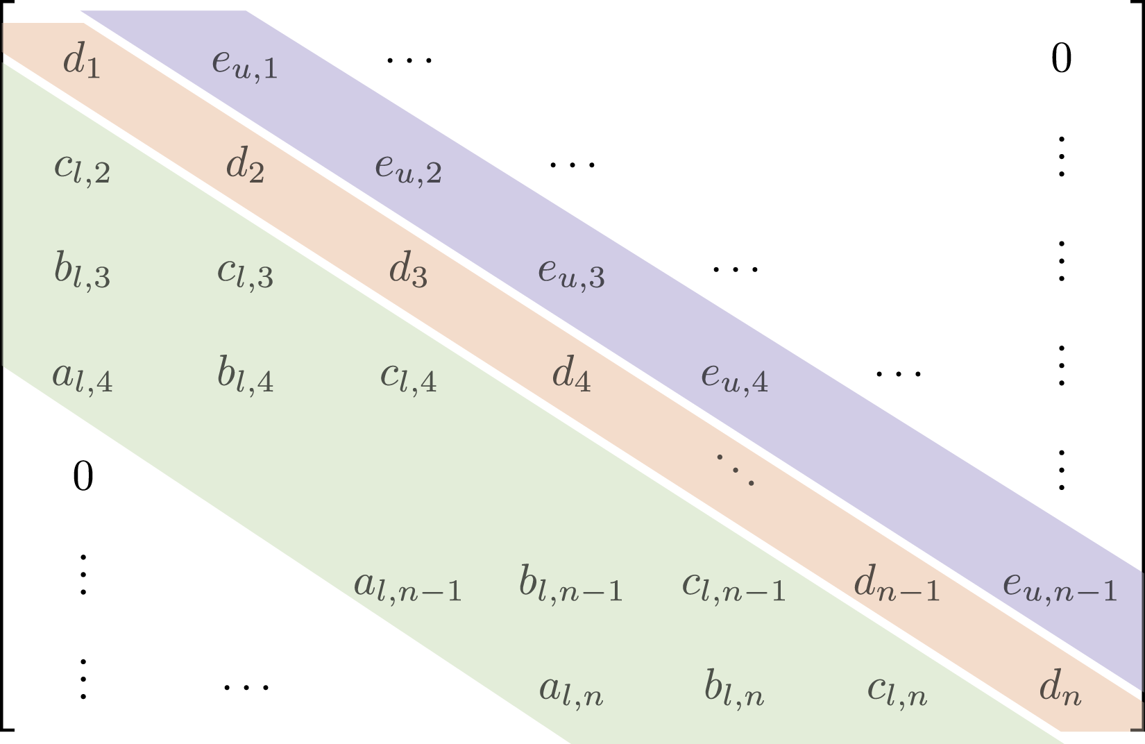$(R^{n \times n})$ with β_L = 3, β_U = 1.

2.1. Ginkgo

Ginkgo is a high-performance numerical linear algebra library that implements efficient and performance portable linear solvers and preconditioners (Anzt et al. (2022)) with support for various hardware backends such as NVIDIA, AMD and Intel GPUs. Ginkgo has also been integrated into different applications such as MFEM, deal.ii, NekRS, SUNDIALS, XGC, enabling these applications to take advantage of the solvers and preconditioners implemented in Ginkgo.

Batched iterative solvers and preconditioners have been added recently to accelerate science applications such as combustion simulations (Aggarwal et al. (2021)) and plasma physics (Kashi et al. (2023)).

2.2. Batched band matrix storage format

Unlike general sparse matrices, the fill-in for band-structure matrices is limited to within the band if no pivoting is used, and the fill-in with partial pivoting is also well-defined, with given lower and upper bandwidths. Storing these band matrices in a tailored format and using their structure to compute the factorization can be advantageous. LAPACK (Anderson (1999)) introduced an efficient storage format for band-structure matrices and a customized solver operating on the band matrix storage format in the LU factorization and the subsequent triangular solves. We visualize the band matrix storage format in Figure 2. As partial pivoting is necessary to ensure stability for a general linear system solver, the storage format allocates additional memory for possible fill-in during the factorization. In Figure 2, we see these locations marked by “+”. The extra padding (elements only stored to ensure uniform strided accesses) is marked with “∗”. The total number of bands stored, each of size n, is equal to β_st = 2β_L + β_U + 1. This includes the extra storage required for possible fill-in introduced by pivoting.

Figure 2.

Band storage 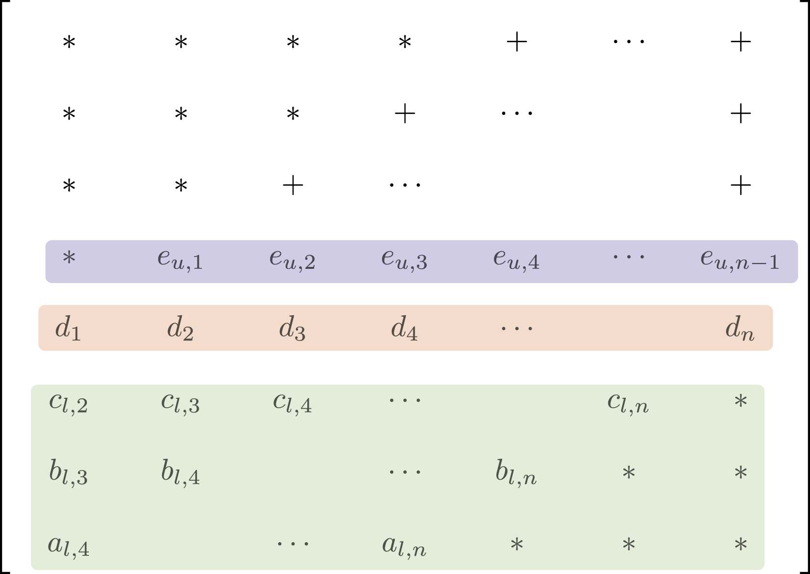$(R^{β_{s t} \times n})$ : Number of elements stored = β_st × n.

2.3. Batched direct solves for band matrices

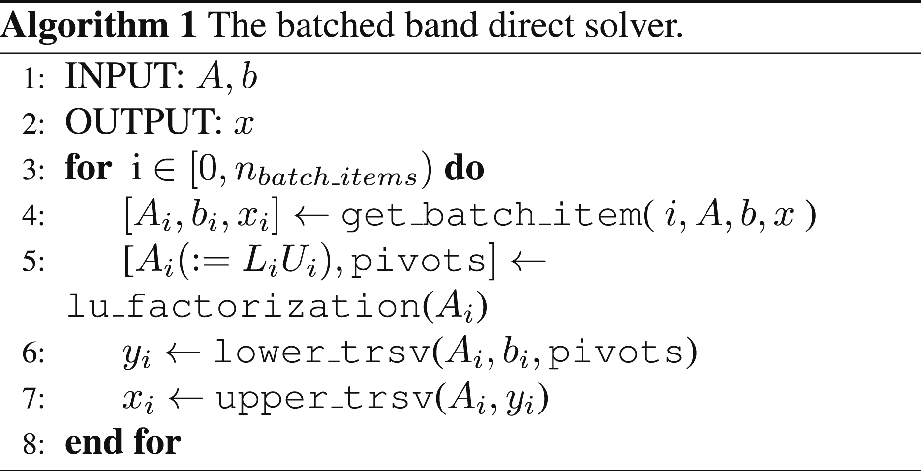
With the band matrix stored as shown in Figure 2, the batched band direct solver consists of two steps: An LU factorization that decomposes a band matrix of the batch into triangular factors, and the subsequent triangular solves using the generated triangular band factors. The batched band direct solver is shown in Algorithm 1.

3. Related work

There have been efforts in developing algorithms for data-parallel basic linear algebra functionality (BLAS) and advanced solver algorithms (LAPACK). The data-parallel versions of the functionality are generally called “batched” to indicate the data-parallel processing of a batch of linear algebra objects. A batched BLAS interface has also been recently proposed (Dongarra et al. (2016; 2017)) to standardize the interface to batched basic linear algebra functionality across hardware architectures and software stacks. This standardization effort for batched functionality has also been expanded to LAPACK, providing direct solvers for dense linear systems (Abdelfattah et al. (2021)).

In terms of batched direct solvers for sparse problems, there has been some work on tridiagonal and penta-diagonal systems (Valero-Lara et al. (2018); Carroll et al. (2021); Gloster et al. (2019)), and the NVIDIA cuSPARSE library provides the gtsv2StridedBatch routine based on variants of cyclic reduction for solution of batched tridiagonal matrices.

These methods aim to solve tridiagonal and penta-diagonal systems and rely on Thomas’ algorithm or cyclic reduction (Valero-Lara et al. (2018)). These implementations are not fine-grain parallel, but each GPU thread solves an entire linear system. The performance benefits, therefore, primarily come from storing the problem data in an interleaved fashion to enable coalesced data access. Coalesced accesses ensure concurrent threads can compute efficiently in a SIMD (single instruction multiple data) fashion, improving throughput. This is suitable for GPUs whose threads have limited co-operative functionality. For modern GPUs, utilizing the co-operative functionality between threads in addition to the SIMD functionality is necessary to provide better performance (NVIDIA (2020)).

In the context of the Human Brain Project (Valero-Lara et al. (2017)), methods similar to cuThomasBatch (Valero-Lara et al. (2018)) have been developed to accelerate the solution of batched Hines systems on NVIDIA GPUs. There also exists some work on the efficient solution of batched penta-diagonal systems (Gloster et al. (2019); Carroll et al. (2021)), however, in these attempts, the factorization step is performed on the CPU, necessitating data transfer for the triangular solves, which are performed on the GPU. Within a non-batched setting, GPU-based tridiagonal solvers have also received some attention (Klein and Strzodka (2021); Pérez Diéguez et al. (2018)).

The development of direct solvers for band matrices with an arbitrary number of sub- and super- diagonals, (β_L, β_U) has received very little attention due to the challenging nature of its implementation. The only implementation that performs a GPU-resident factorization and solve for band matrices that the authors could find at the time of writing this paper is the implementation available in the MAGMA library (Abdelfattah et al. (2023)). For the CPU, LAPACK provides efficient routines (xgbsv) (Blackford and Dongarra (1991)) that can be launched in a data-parallel fashion by launching a solver routine on each of the CPU cores and each solver instance solving a subset of the linear systems in the batch. Additionally to the high-level parallelization across the systems in the batch, vendor implementations of LAPACK such as Intel MKL (Intel (2023)) may use SIMD vectorization to harness the available parallelism within a single CPU core for increasing the performance of the solver instances launched on the distinct cores.

4. Batched band solvers in Ginkgo

In this paper, we extend the batched solver functionality in Ginkgo with GPU-resident batched band solvers for arbitrary band sizes, and specializations for wide bands and tridiagonal matrices.

Ginkgo employs the standard LAPACK band matrix format shown in Figure 2. To ensure coalesced access, Ginkgo stores the matrix band arrays in a column-major format without interleaving the elements of different matrices. This has proven to be efficient for both GPU and CPU implementations of band solvers (Abdelfattah et al. (2023)).

As our focus is on small problems and the goal is to solve thousands to hundreds of thousands of small problems in parallel, we map one linear system solve (factorization + triangular solves) to one workgroup (thread block) of the GPU. As workgroups have no data dependencies, this allows for the parallel and independent processing of the problems, and global memory reads and writes are conflict-free, thereby reducing the global memory contention.

Due to the reduced amount of parallelism available in the band solver, large work-group sizes would lead to warp-stalling (A warp is similar to a SIMD unit in CUDA, consisting of 32 threads that execute the same instruction). We therefore tune our workgroup sizes based on the problem size and the matrix bandwidth. An additional advantage of small workgroup sizes is that more batch items can be processed concurrently, allowing for higher throughput.

For the efficient solution of batched band linear systems, we perform the triangular solves for each system immediately after the factorization. i.e., once a band matrix is loaded into the multiprocessor memory, we first perform in-place factorization and then the forward and backward triangular solves in shared memory without writing intermediate results to the GPU main memory. While this requires consolidating both functionalities into a single GPU kernel it radically reduces the main memory access. In the end, we launch a single kernel handling the solution of all linear systems in the batch.

Next, we provide more details on our generic band solver implementation. Afterward, we present the implementations tailored towards matrix batches with wide bands and batches composed of tridiagonal matrices.

4.1. Batched LU factorization for band matrices

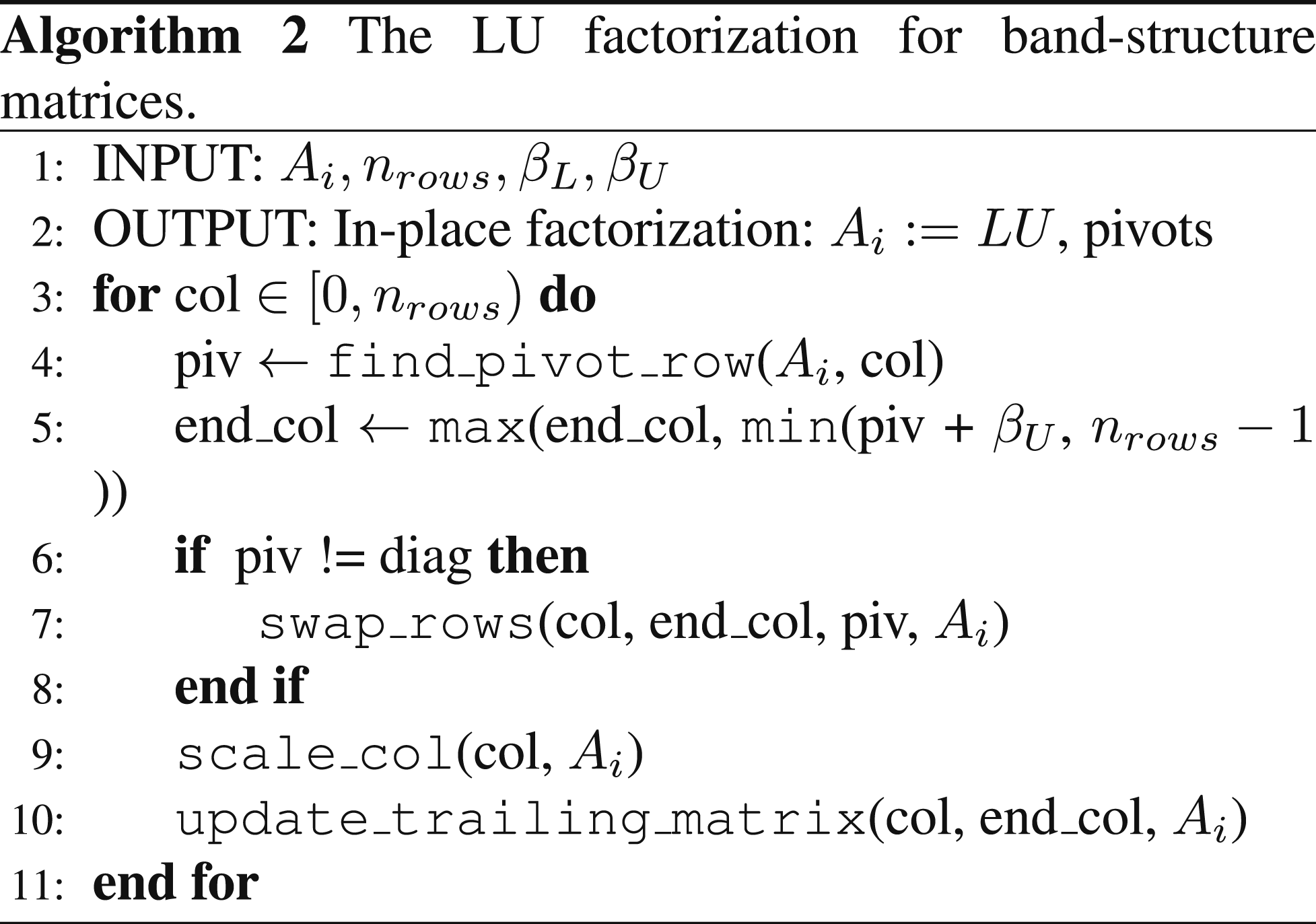
The LU factorization of a band matrix batch is shown in Algorithm 2. For each batch item, we process each column individually. First, we identify the pivot and process the row swaps. We then proceed by scaling the columns and finish by updating the trailing matrix. After completion, we have an in-place factorization of the input band-matrix. We note that as a result of the storage scheme shown in Figure 2, we do not need to perform a structural analysis or allocate additional memory to account for fill-in.

Templating each kernel on a compile-time subwarp size, we can maximize SIMD parallelism and ensure that accesses to the band matrix are coalesced.

4.2. Batched triangular solves

After computing a factorization, we need to perform two triangular solves.

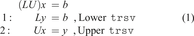
\begin{aligned} (L U) x & = b \\ 1 : L y & = b, Lower t r s v \\ 2 : U x & = y, Upper t r s v \end{aligned}

(1)

With partial pivoting (only row interchanges), the lower triangular solver uses the pivoting array computed in the factorization step, while pivoting is not required for the upper triangular solve.

Both triangular solves are processed row-by-row: the upper triangular solve uses backward substitution, and the lower triangular solve uses forward substitution.

4.3. Efficient solution of wide-band matrices

For matrices with small to medium bandwidths ((β_L + β_U) < 32, with all elements of a row fitting inside a warp), processing each column is efficient, as it enables coalesced access when performing the scaling and the trailing matrix updates. For matrices with a wide band, due to the larger number of elements that need to be updated in each row, performing a blocked factorization and processing ϕ columns at once, where ϕ is the panel size, can be advantageous.

For wide-band matrices, processing more columns in a paneled fashion provides better overall concurrency as a result of reduced stalls for executing warps. In this case, the dependencies restricted to within one warp, thereby removing the need for cross-warp synchronizations. If we were to process one column per thread, then we would need more than one warp per row ( $>$ 32 elements per row), creating dependencies between warps, leading to more warp stalls, thereby reducing the overall GPU utilization.

A schematic of our panel-based factorization is shown in Figure 3 for a panel size of 2. We partition the matrix into block-diagonal $(A_{00} \in R^{ϕ \times ϕ})$ , trailing row block $([A_{01} A_{02}] \in R^{ϕ \times (ϕ_{1 j} + ϕ_{2 j})})$ , trailing column block $([\begin{matrix} A_{10} \\ A_{20} \end{matrix}] \in R^{(ϕ_{1 k} + ϕ_{2 k}) \times ϕ})$ and a trailing block-diagonal block $([\begin{matrix} A_{11} & A_{12} \\ A_{21} & A_{22} \end{matrix}] \in R^{(ϕ_{1 k} + ϕ_{2 k}) \times (ϕ_{1 j} + ϕ_{2 j})})$ as shown in equation (2), with ϕ_1k, ϕ_2k, ϕ_1j, ϕ_2j as defined in Algorithm 3 (the trailing size of the blocks).

A = [\begin{matrix} A_{00} & A_{01} & A_{02} \\ A_{10} & A_{11} & A_{12} \\ A_{20} & A_{21} & A_{22} \end{matrix}]

(2)

Figure 3.

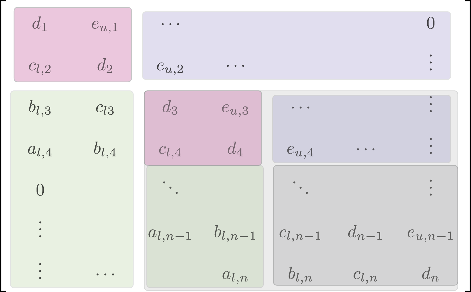
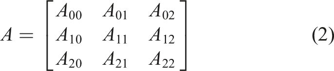
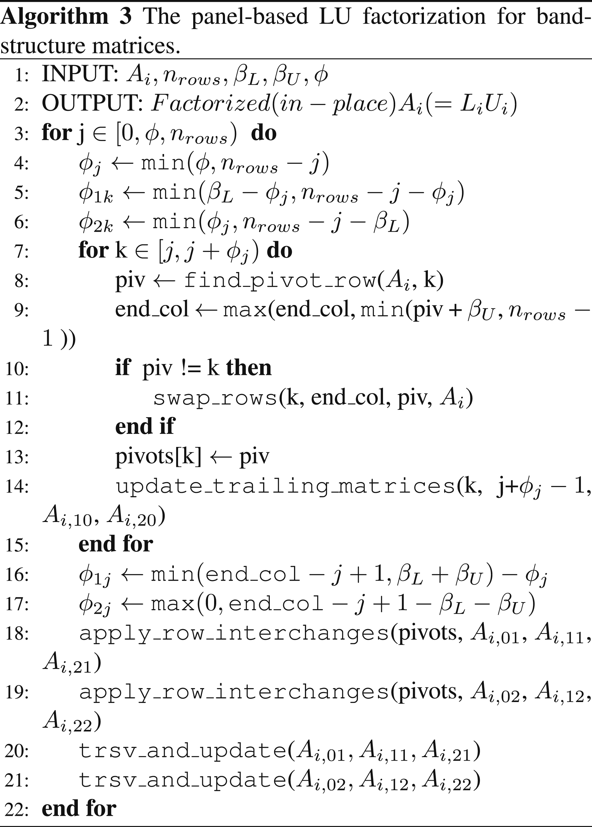
Panel factorization for band matrix ( $\in R^{n_{rows} \times n_{rows}}$ ) with β_L = 3, β_U = 1, ϕ = 2.

The panel LU factorization algorithm, shown in Algorithm 3, proceeds by first factorizing the column panel $[\begin{matrix} A_{00} \\ A_{10} \\ A_{20} \end{matrix}]$ . We compute the row pivots, and update the trailing block columns A₁₀ and A₂₀. Using the computed pivots, we apply the necessary row interchanges in a block-column fashion. Using a trsm and trailing column update, we update the block columns for A₀₁ and A₀₂.

We proceed in this fashion recursively for the trailing block diagonal matrix until the entire matrix has been factorized. As the factors replace the original matrix in memory, we consider it an in-place factorization.

To ensure coalesced accesses when processing ϕ columns at a time, we utilize a workspace array to copy the matrix blocks that tend to have non-coalesced accesses, namely A₀₂ and A₂₀. We omit this implementation detail from Algorithm 3 for simplicity.

4.4. Efficient solution of tridiagonal matrices

Tridiagonal matrices are a special case of band matrices with (β_L, β_U) = (1, 1). For these systems, it is not necessary to compute an LU factorization, but we can directly use the Thomas algorithm to solve the linear system (Valero-Lara et al. (2018)). A recursive divide-and-conquer approach allows for a high level of concurrency (Wang and Mou (1991)). We use this approach for the batched tridiagonal solver and show that our implementation is faster than both the vendor-provided tridiagonal solver implementation and the general band solver implementation.

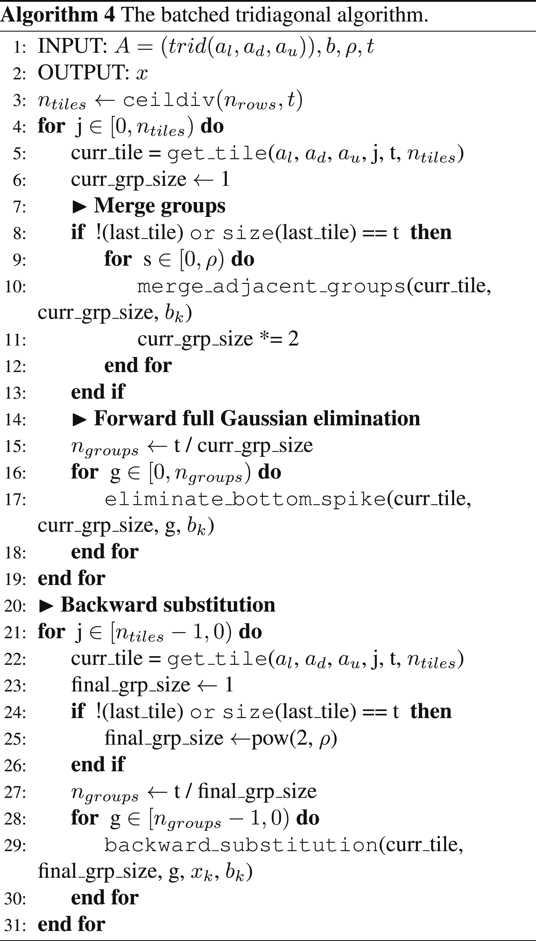
The algorithm we use (shown in Algorithm 4) is a variant of the standard parallel Gaussian Elimination (GE) for tridiagonal matrices (Wang and Mou (1991)). The idea is to first merge adjacent rows into groups, with a partial GE, removing dependencies between the adjacent groups. We then obtain groups that can be eliminated in parallel with a full GE step. Once all groups have been eliminated with a forward GE, we can perform a backward substitution to obtain the final solution. A schematic of this process is shown in Figure 4 for ρ = 2 where ρ is the number of merge steps that is performed on the initial matrix and for a tile size, t = 16.

Figure 4.

Divide and conquer parallel Gauss-Elimination algorithm for tridiagonal matrices with number of merge steps, ρ = 2 and tile size, t = 16. (a) Initial matrix (b) Merge groups (c) Eliminate group 1 (d) Eliminate group 2 (e) All groups eliminated (f) Final solution.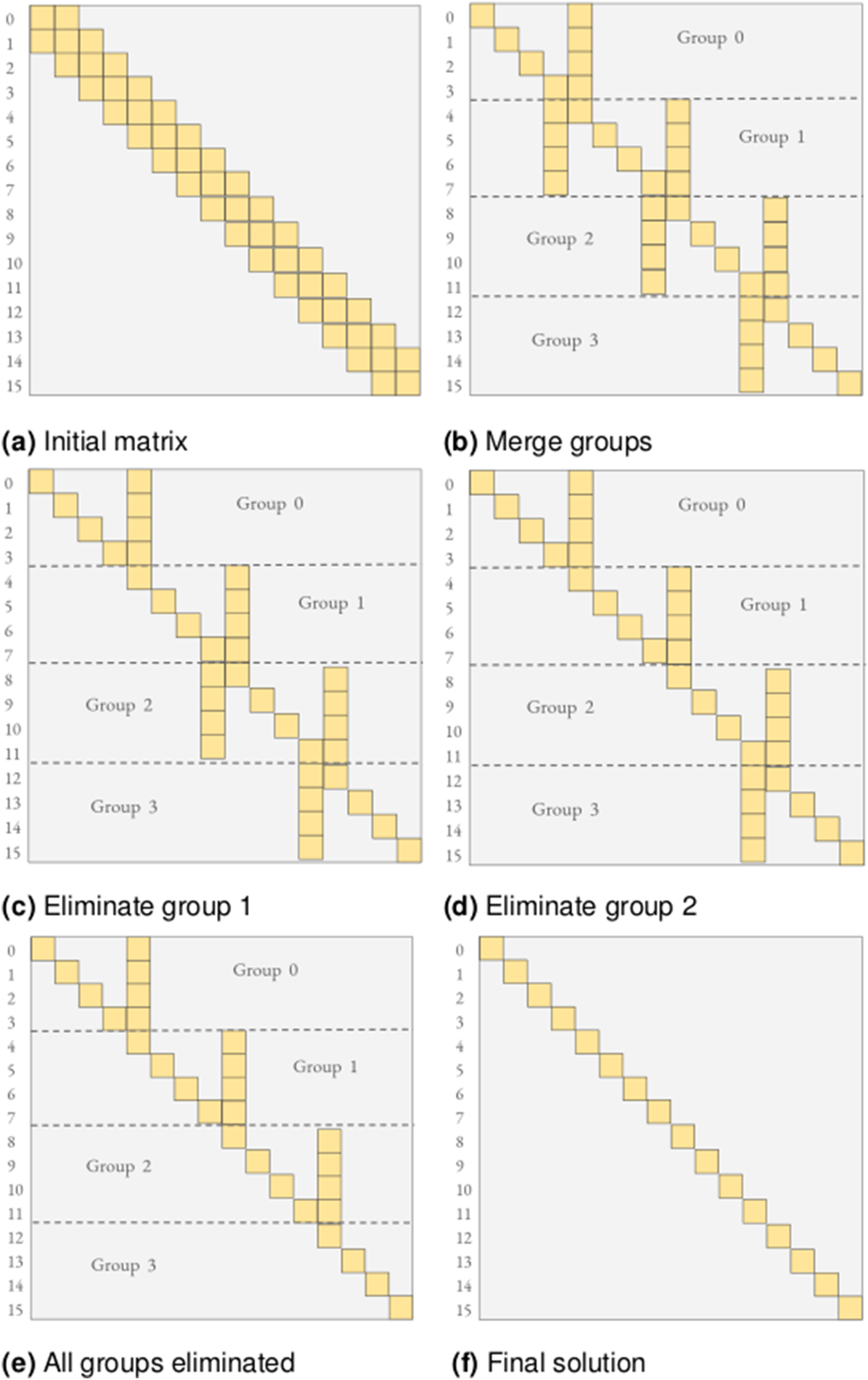

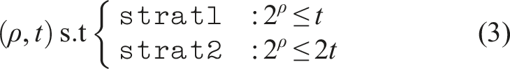
To optimize performance, we expose two control knobs to the user. The tile size, t, defines the size of the matrix tile to be handled by each subwarp, and the number of merge steps, ρ, defines the total number of groups that are created and forward-eliminated in parallel. Additionally, the user can choose one of two strategies: Each thread in a subwarp handles one row of the matrix (strat1), or each thread in a subwarp handles 2 rows of the matrix (strat2). Therefore, we can obtain (ρ, t) from the constraints:

(ρ, t) s.t \{\begin{cases} s t r a t 1 & : 2^{ρ} \leq t \\ s t r a t 2 & : 2^{ρ} \leq 2 t \end{cases}

(3)

To simplify usage, we also provide a strategy, auto, that automatically sets (ρ, t) depending on the number of rows, n_rows, as that forms the central aspect when choosing (ρ, t). A higher value of ρ implies more concurrency available in the forward-elimination step as the partial GE creates more merge groups: ρ = 2 creates 2² number of groups after the partial GE step. Increasing the value of ρ also increases the cost of the partial GE step as more rows need to be eliminated. The tile size t determines the maximum size of the matrix tile on which the second elimination step can be performed. The maximum tile size is set to 32 (the warp size) to enable use of the efficient warp-level communication functions. For matrices which are larger (n_rows > 32), we set the tile size to 32, and calculate ρ such that the condition in equation (3) is satisfied.

As the choice of ρ defines the subwarp size to be used, and the value of ρ depends on the problem size (n_rows), we instantiate kernels for all major subwarp sizes (1, 2, 4, 8, 16, 32: powers of 2, upto the warp size of 32) during compile time. The optimal subwarp size is selected at runtime, depending on the problem size (n_rows). As each subwarp handles one matrix tile of size t, we can utilize co-operative group functionality such as warp-shuffles and broadcasts (Tsai et al. (2021)) for efficient in-register and local memory operations (involved in the GE steps), which reduces the overall global memory traffic.

5. Benchmarking and performance evaluation

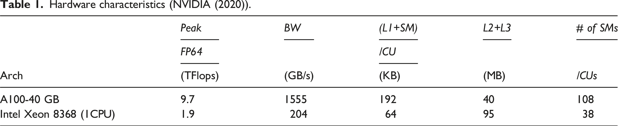
We use the HoreKa¹ supercomputer for the performance evaluation of our batched band solvers. It consists of 4 NVIDIA A100 GPUs per node and 2 sockets of Intel Xeon Platinum (Icelake) CPUs with a total of 76 CPU cores per node. The relevant hardware characteristics are shown in Table 1.

Table 1.

Hardware characteristics (NVIDIA (2020)).

Arch	Peak	BW	(L1+SM)	L2+L3	# of SMs
	FP64		/CU		/CUs
	(TFlops)	(GB/s)	(KB)	(MB)	/CUs
A100-40 GB	9.7	1555	192	40	108
Intel Xeon 8368 (1CPU)	1.9	204	64	95	38

5.1. Dataset and evaluation metrics

Our dataset consists of artificially generated band matrices with random values (from a normal distribution) that are different along three main characteristics: the lower bandwidth β_L, the upper bandwidth β_U, and the diagonal dominance. For each of the experiments², we run 2 warmup iterations to minimize the effects of startup artifacts such as library and symbol loading, data transfer, etc., and gather average timings over 5 kernel executions. We verified (post-solve) that all variants of the solvers (our solvers and the ones compared with) converged to machine precision (10⁻¹⁶).

To ensure a fair comparison of the solvers, we exclude the setup and analysis timings and only report the timings for the solution process (factorization and solve).

We present the performance of Ginkgo’s batched solvers on one A100 GPU with CUDA 11.8. For comparison with the CPU-based banded solvers, we use the LAPACK implementation from Intel MKL 2022.0.2 with the Intel C/C++ compiler 2021.5, and parallelize over all the available CPU cores (the full CPU node, 76 cores) using OpenMP. Additionally, we compare our performance with MAGMA (Dongarra et al. (2014)), a state-of-the-art software that implements both batched and non-batched BLAS and LAPACK routines for GPUs.

We use MAGMA’s asynchronous batched strided interface. As mentioned previously, we do not include the timings for allocation and deallocation of MAGMA’s workspace. Both the MAGMA and MKL interfaces perform an in-place factorization, while Ginkgo’s factorization ensures the immutability of the input matrix and copies the band matrix into a workspace before each solve. The time needed for this explicit copy is included in Ginkgo’s overall runtime.

The number of batch items in the experiments varies with the number of nonzeros in each of the batch items. To minimize effects of the CUDA runtime, we set the number of batch items to a sufficiently high enough count that fills the GPU memory and is reflective of the application use-case.

5.2. Batched band solvers on GPUs

We first present the performance of Ginkgo’s batched band solvers for two sets of matrix band sizes, (β_L, β_U) = (2, 3) and (β_L, β_U) = (15, 5), representing matrices with narrow and medium band sizes. Figure 5 shows the time to solution for the three batched band solvers: The CPU-based solver using Intel MKL, Ginkgo’s batched band solver, and MAGMA’s batched band solver (Abdelfattah et al. (2023)), for matrix sizes ranging from (32 × 32) to (1024 × 1024) for a total of 10⁴ linear systems. Both Ginkgo’s and MAGMA’s GPU batched band solvers outperform the batched CPU band solver. The MAGMA implementation is dependent on the amount of shared memory available on the GPU and explicitly performs the factorization and the solve after copying the band arrays to the GPU shared memory. Therefore, we observe the jump in timings at a matrix size of (128 × 128) where the shared memory capacity is exceeded and only part of the work vectors can be stored in shared memory. We do not observe this behavior for Ginkgo’s implementation because it caches only the pivot vector in shared memory but keeps the band array in global memory. This strategy allows for increasing the occupancy of the GPU, allowing the CUDA runtime to utilize the caches efficiently, based on the thread block sizes.

Figure 5.

Ginkgo band solver runtime (in seconds) with increasing matrix size (n_rows) on a A100 GPU versus MKL + OpenMP on Intel Icelake (76 cores) and MAGMA (on A100 GPU), with 10⁴ batch items. For matrices with narrow bands (left), 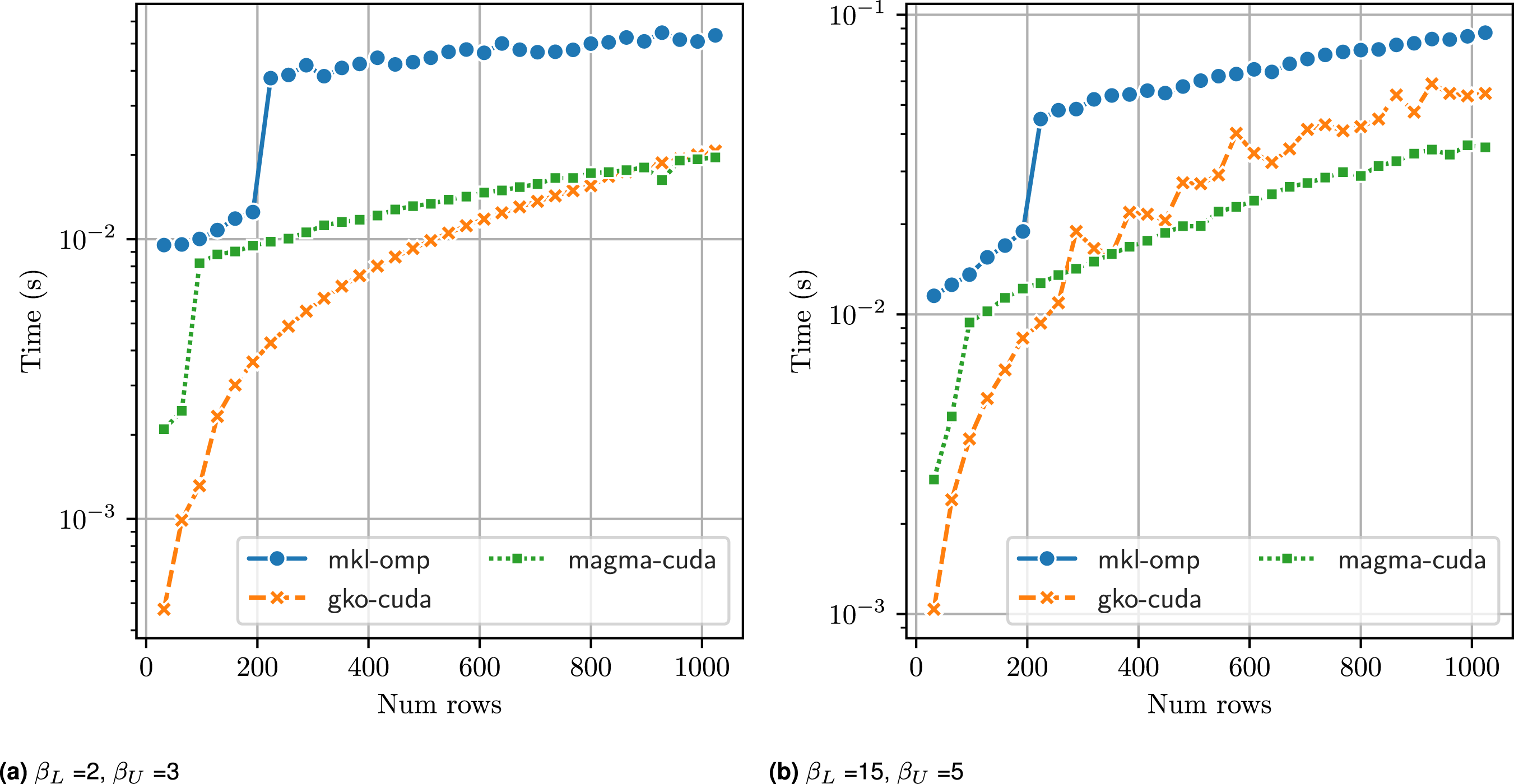Ginkgo performs better than MKL and MAGMA. For matrices with wider bands (right), Ginkgo is the best for sizes upto 256, but MAGMA performs the best for larger sizes. (a) β_L =2, β_U =3 (b) β_L =15, β_U =5.

Due to the limited amount of parallelism available in the band LU factorization, large thread block sizes are inefficient as they leave most warps unutilized. For the non-blocked factorization, Ginkgo’s solver uses only a single workgroup for each system in the batch. This allows leveraging the coarse-grained parallelism of the GPU, enabling better scaling when solving batches with large cardinality. This comes at the cost of lower performance for large problems as seen in Figure 5(a), where more data needs to be fetched from global memory.

Increasing the sizes of the bands of the matrices, as shown in Figure 5(b), with (β_L, β_U) = (15, 5), we see a similar behavior: MAGMA’s batched band solvers perform the best, particularly for matrix sizes larger than (256 × 256). There, in addition to increased shared memory usage, it is beneficial to increase the amount of fine-grained parallelism available.

Figure 6 shows the solver runtime for Ginkgo’s batched band solver in comparison to Intel’s MKL LAPACK band solver parallelized with OpenMP. We see that the GPU based solvers are more efficient for small batch sizes, and hence have a higher relative speedup. The variance in the plot denotes the different linear system sizes (number of rows in the system matrix), with the solid line showing the median runtime over the different matrix sizes, ranging from (64 × 64) to (1024 × 1024).

Figure 6.

Runtime comparison of 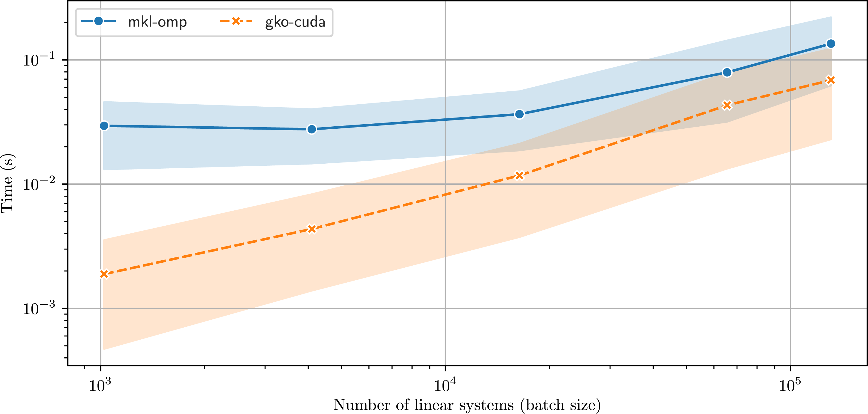Ginkgo band solver (on A100 GPU) and MKL + OMP on (Intel Skylake CPU, 76 cores) for different batch sizes with fixed matrix band widths, β_L = 2, β_U = 3. Ginkgo’s band solver performs better than the MKL solver for all different batch sizes.

5.3. Wide band matrix optimizations

In Figure 7, we run the batched band solvers for matrices with a large bandwidth, (β_L, β_U) = (32, 32). These wide bands can occur in applications such as the XGC plasma simulations (Ku et al. (2009)). As noted before, using a non-blocked version of the factorization does not allow for harnessing the parallelism available, and we see in Figure 7 that the non-blocked version on the GPU achieves lower performance than CPU-based MKL solver. With a blocked version, Ginkgo’s GPU solver outperforms both the MKL and MAGMA solver.

Figure 7.

Runtime comparison of 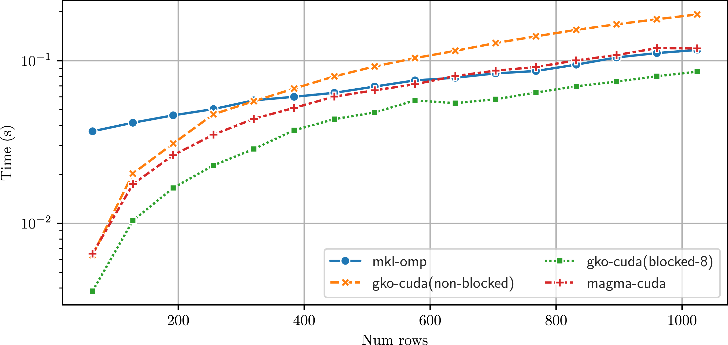Ginkgo’s block band solver (on a A100 GPU) for wide band matrices, β_L = 32, β_U = 32 with increasing matrix size (n_rows), with 5000 number of batch items, using a block size, ϕ = 8. The runtime of MAGMA (on a A100 GPU) is comparable to that of MKL (on 76 cores of Intel Skylake). Ginkgo’s non-blocked solver (which processes one column at once) is not efficient, but the blocked-solver, using a block size of (8 × 8) performs better than both MKL and MAGMA for all matrix sizes.

5.4. Tridiagonal matrix optimizations

A pathological case for the band solvers is a tridiagonal matrix. With only one sub- and super- diagonal, it does not offer enough parallelism to be solved with a general band solver algorithm like in LAPACK. We therefore implement a specialized tridiagonal solver as explained in Section 4, based on the parallel divide-and-conquer approach (Wang and Mou (1991)). Figure 8(a) shows the runtimes of Ginkgo’s batched tridiagonal solver compared with both cuSPARSE’s batched tridiagonal solver, and with Ginkgo’s generic band solver, setting (β_L, β_U) = (1, 1).

Figure 8.

Runtime (in seconds) of 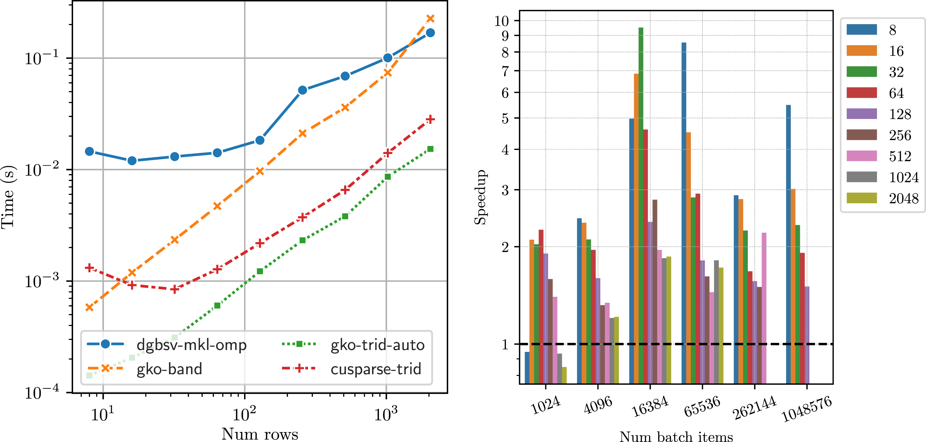Ginkgo’s tridiagonal solver on a A100 GPU versus MKL + OpenMP on Intel Icelake (76 cores) and cuSPARSE (on A100 GPU), with increasing matrix sizes and 65,536 batch items (left, (a)), and speedup versus cuSPARSE for different batch sizes and different matrix sizes (right, (b)). The tridiagonal solvers perform significantly better than the generic band solvers of MKL. Ginkgo’s tridiagonal solvers are also faster than cuSPARSE’s batched tridiagonal solvers.

Ginkgo automatically selects the best parameters (tile size, t and number of merge steps, ρ) for the tridiagonal solver based on the number of rows of the matrix to maximize the available parallelism on the GPU. We see that there is a significant benefit in using a tailored tridiagonal solver rather than using the band solver for tridiagonal matrices, with the tridiagonal solver outperforming the GPU-based band solver by almost 10 × . The merge-tiling-based approach outperforms the cuSPARSE batched tridiagonal solver by 1.7× on average.

Figure 8(b) shows the speedup obtained by Ginkgo’s batched tridiagonal solver over cuSPARSE for different batch sizes. We note that for the cuSPARSE solver, we time only the solve phase and do not consider the analysis phase. We observe that the merge-based tiling approach is more efficient for large batch sizes due to the better latency hiding of the warp scheduler for these larger batch sizes. Additionally, for small problems, Ginkgo performs significantly better, for example with an average speedup of over 3× for a matrix size of (8 × 8). For larger problems, Ginkgo still outperforms the cuSPARSE solver with an average speedup of 1.5×. We note that the cuSPARSE solver exceeds the memory capacity of the NVIDIA A100 GPU for some matrix sizes, and these results are therefore not shown in the graph.

5.5. Effects of pivoting

To ensure the robustness of the LU factorization, pivoting is usually necessary. For almost all cases, partial pivoting (row interchanges) is sufficient to ensure the stability of the factorization (Duff et al. (2017)). The state-of-the-art banded solvers such as MKL and MAGMA also implement only partial pivoting.

While pivoting is necessarry for stability of the algorithm, it can adversely affect performance. Partial pivoting, for instance consists of row interchanges to ensure that the largest element in a row is the diagonal element. This can have adverse effects, particularly increasing cache misses between subsequent operations before and after pivoting. It is therefore of interest to understand the effect of pivoting on the algorithm runtime.

Our dataset consists of matrices with all elements sampled from a normal distribution with variance of 0.1. All band solver implementations are equipped with partial pivoting. In Figure 9(a), we consider four experiment runs of the band solver and measure the number of row interchanges in each of the batch items for two matrix sizes. We see that with a random matrix generation approach, with approximately equal elements sampled from a normal distribution, all batch items need to perform partial pivoting and the number of row interchanges across the batch items ranges from $(n_{rows} - \sqrt{n_{rows}} / 2)$ to n_rows, where n_rows denotes the number of rows in each matrix of the batch.

Figure 9.

Effect of pivoting on performance: (a) variation in number of row interchanges in a batch, (b) Comparing runtime (in seconds) of the band solvers (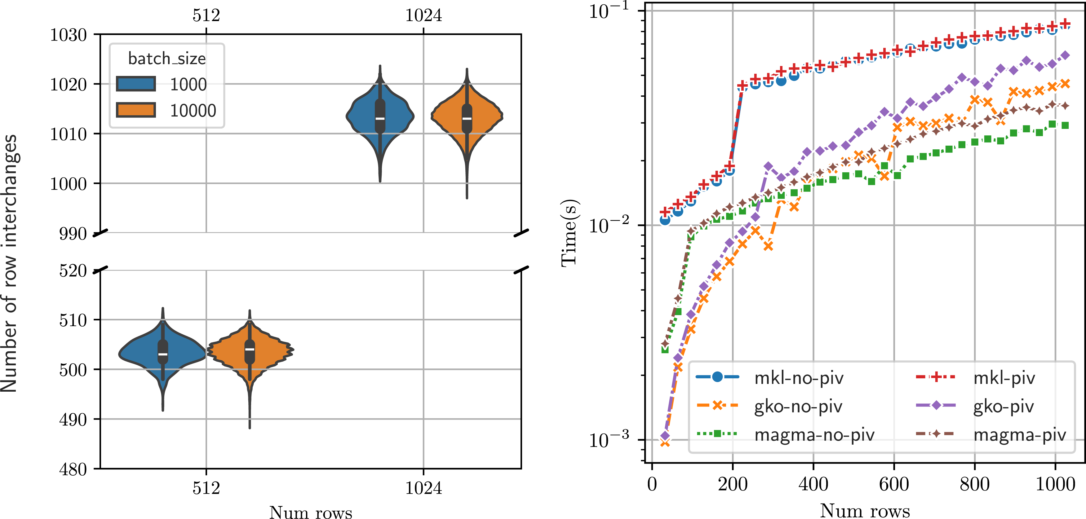Ginkgo, MAGMA and MKL) with and without pivoting, β_L = 15, β_U = 5, with 10⁴ batch items. The GPU solvers (Ginkgo and MAGMA) are affected more by the necessary pivoting than the CPU solver (MKL) due to the larger caches available on CPUs.

Figure 9(b) shows the runtime of the solvers with and without partial pivoting. To ensure that the band solvers do not apply row exchanges, we explicitly make the matrices strictly diagonally dominant by increasing the weight of the diagonal to be such that $| a_{j j} | > \sum_{i}^{n_{rows}} | a_{i j} |$ . For the CPU-based MKL solver, the runtime overhead of pivoting is small – which is expected, given the significantly larger and coherent caches (L2 and L3). The GPU solvers from MAGMA and Ginkgo both execute faster when no pivoting is necessary. Conversely, if pivoting is necessary, the communication across warps and induced synchronization introduces significant performance penalties. With partial pivoting, we also incur more cache misses, leading to more fetches from the main memory resulting in reduced performance for both MAGMA and Ginkgo solvers. Figure 10 shows the speedup of the solvers without pivoting over the ones that need pivoting for different matrix sizes. As expected, the benefits of omitting pivoting grow with the matrix size.

Figure 10.

Band solver speedup without pivoting (ratio of solver runtimes with and without pivoting), β_L = 15, β_U = 5, with 10⁴ batch items. The GPU solvers (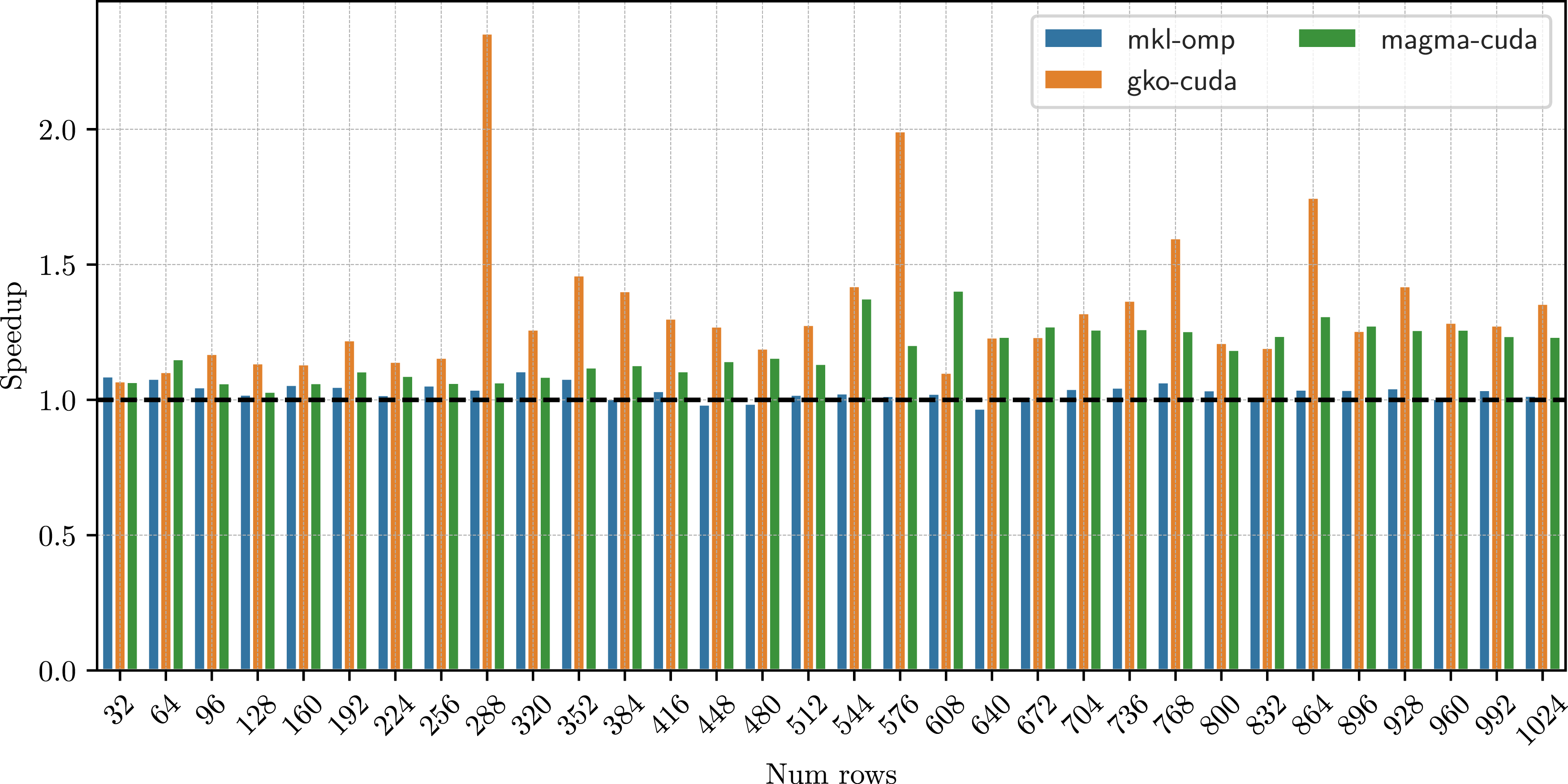Ginkgo and MAGMA) have a larger speedup when pivoting is not necessary. Larger matrix sizes have a more pronounced benefit when pivoting is not necessary.

We note that the code for the two experiments is identical. The only difference is in the input data: the matrices are generated such that pivoting is not necessary. Therefore, the end-user automatically gets improved performance when the matrix does not require any pivoting.

5.6. Linear systems from a plasma physics application

Finally, we study the performance of Ginkgo’s batched band solvers for matrices from the XGC plasma physics application. XGC (Hager et al. (2016)) is a 5D gyrokinetic particle-in-cell (PIC) application code that numerically simulates fusion plasma for realistic geometries, and has been optimized for boundary plasma. A nonlinear collision operator for the Coulomb collisions is required to accurately model edge plasma. Using a Fokker-Planck-Landau operator in the 2D guiding-center velocity space for multiple particle species, XGC employs a backward Euler time integrator to evolve the distribution functions for the multiple species in time.

Each time-step therefore requires multiple non-linear steps and each non-linear step requires multiple independent linear solves, giving us a batched linear system for each species. XGC currently uses the band solver from vendor-provided LAPACK, mapping one linear system to one CPU core using Kokkos (Carter Edwards et al. (2014)).

The size and characteristics of the band matrix are dependent on the velocity grid used. For example, using a velocity grid of size (31 × 32) gives a matrix of size (992 × 992). Additionally, if multiple species are involved, we need to solve a linear system for each of these species. For our purposes, we use a velocity grid of size (31 × 32) and two species: ions and electrons. The characteristics of our test matrices (obtained from the XGC application) are shown in Figure 11. We note that the matrix is derived from a 9-point stencil, therefore the upper and lower bandwidths are given by (β_L, β_U) = (33, 33), dictated by the number of points in the x-direction of the velocity grid. The matrix therefore has a moderately large bandwidth. The number of batch items varies with the number of species, and can depend on the available GPU memory. In a typical run of XGC (on A100-40 GB), it can vary from 256 to 1024. It is expected that for newer GPUs with larger memory capacities, this can be significantly larger.

Figure 11.

XGC example matrix characteristics for the two species, ion and electron (Kashi et al. (2022)). Both species have the same sparsity pattern, but values stored are different. The figure on the right shows the eigenvalues for one such system matrix, for the ion and the electron species. (a) Sparsity pattern (b) Eigenvalues.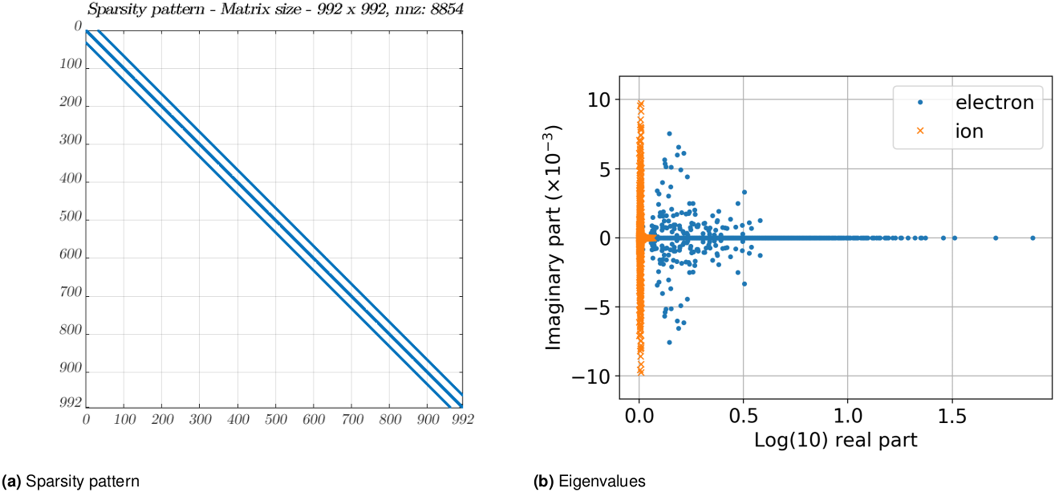

In Figure 12, we compare the performance of our batched band solvers with that of the state-of-the-art CPU-based band solver from MKL on Intel CPUs and with the GPU batched band solvers from MAGMA. Given the wide bandwidth of this matrix, we observe that the non-blocked strategy is inefficient and each subwarp gets assigned too much work, and hence it is slower than both the MKL version and MAGMA. Using a blocked version, with a panel size ϕ = 2, we can improve our performance significantly, outperforming MKL solver on average by 1.5 × . The matrix has lower and upper bandwidths of 33, and we observe that a panel size of 8 gives the best performance, providing a good balance between the amount of work assigned to each subwarp while providing enough parallelism to have enough concurrent warps resident on the compute unit. On average, with a panel size of 8, we get a speedup of 2.5× over the MKL solver. We did not observe any performance benefits beyond a panel size of 8.

Figure 12.

Performance of the batched band solvers with matrices and right hand sides from the plasma physics application, XGC. The left figure shows the runtime (in seconds) for the different batched band solvers for increasing batch sizes. As the matrices have a wide band (33), the blocked version of the 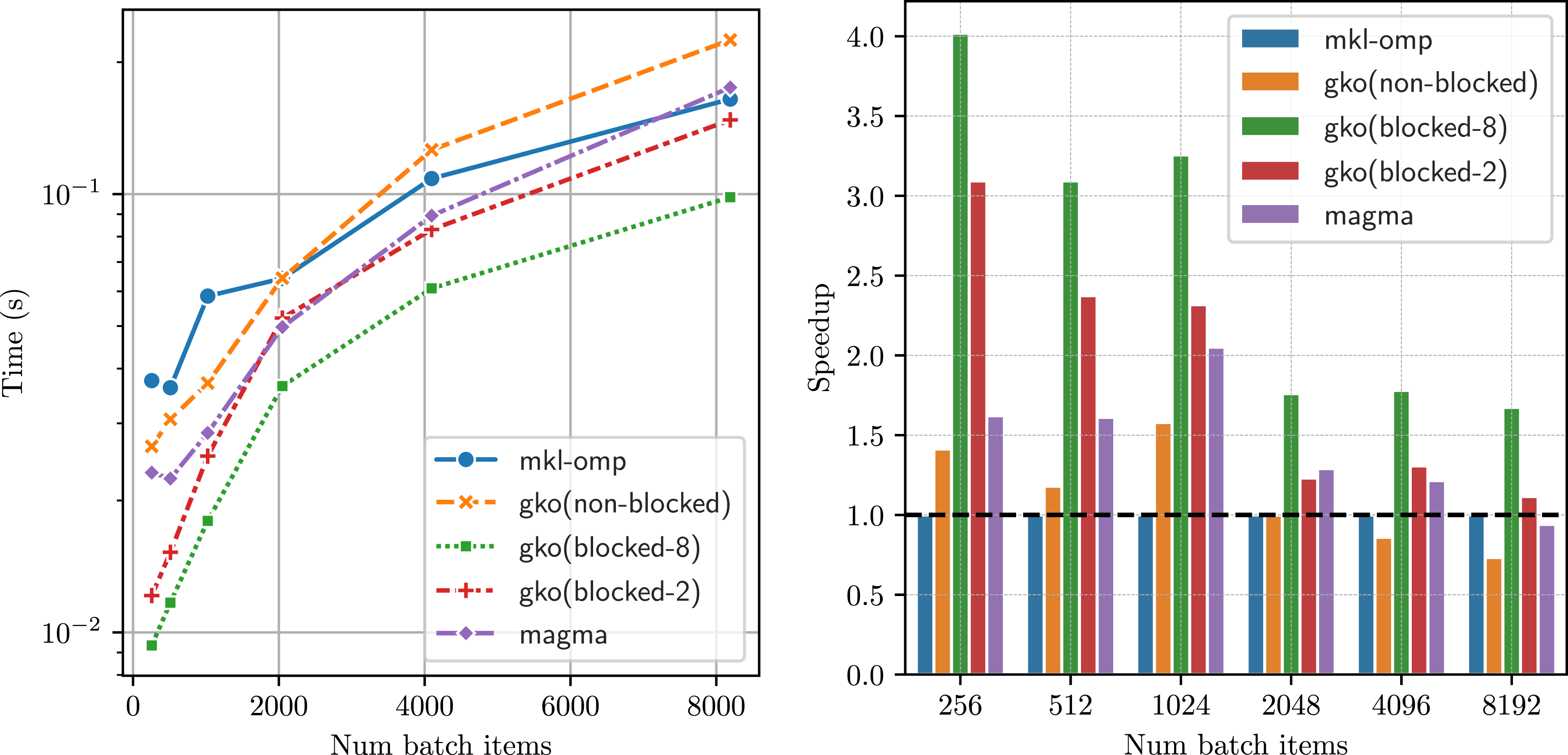Ginkgo band solver (with block size 8) performs the best. The figure on the right shows the speedup of the GPU solvers (Ginkgo and MAGMA) compared to the MKL band solver on the CPU.

6. Conclusion

In this paper, we have presented Ginkgo’s batched band solvers which are useful in many computational physics applications. Using a matrix storage scheme initially proposed in LAPACK, we designed two algorithms for the solution of batched band solvers. The first band solver is efficient for small bandwidth matrices. The second algorithm, a blocked version, uses a panel-based factorization to enable an efficient factorization for matrices with a wide band. We showcased the performance of our batched band solvers for randomly generated band matrices for different bandwidths, and demonstrated competitiveness with the state-of-the-art batched band solvers for CPU and GPU architectures. We included an analysis of the performance impact of partial pivoting, and showed that the GPU solvers can benefit from matrices that do not require partial pivoting.

The third algorithm we presented employed a divide-and-conquer approach for the solution of batched tridiagonal systems. This strategy proved to be significantly faster than implementations available in the software stack provided by hardware vendors.

Finally, we investigated the performance of the developed batched band solvers when applied to linear systems originating from the XGC plasma physics application. We demonstrated attractive runtime savings over the solvers available in MKL and the GPU library MAGMA.

Footnotes

Acknowledgements

We would like to thank Paul Lin and Dhruva Kulkarni from LBNL for providing us with the matrices from the plasma physics application, XGC. This research was supported by the Exascale Computing Project (17-SC-20-SC), a collaborative effort of the U.S. Department of Energy Office of Science and the National Nuclear Security Administration. This work was performed on the HoreKa supercomputer funded by the Ministry of Science, Research and the Arts Baden-Württemberg and by the Federal Ministry of Education and Research, Germany.

Declaration of conflicting interests

The author(s) declared no potential conflicts of interest with respect to the research, authorship, and/or publication of this article.

Funding

The author(s) disclosed receipt of the following financial support for the research, authorship, and/or publication of this article: Basic Energy Sciences (17-SC-20-SC), Bundesministerium für Bildung und Forschung.

ORCID iDs

Pratik Nayak

Hartwig Anzt

Notes

Author biographies

Pratik Nayak is a research scientist at Technical University of Munich. He obtained his PhD from Karlsruhe Institute of Technology in the Computer Science and Applied Mathematics. His research interests include numerical linear algebra, algorithms and data structures for large scale distributed computing, and sustainable software development. In his efforts to further sustainable software, he contributes to many open-source scientific software libraries and he is also a core developer of the Ginkgo linear algebra library.

Isha Aggarwal was a research assistant at Karlsruhe Institute of Technology, Germany. She is currently pursing MBA in the Paris area. She obtained her Bachelors in Computer Science from the Indian Institute of Information Technology, Sri City, India and worked as a researcher in HPC and numerical linear algebra for 1 year at KIT.

Hartwig Anzt is the Chair of Computational Mathematics at the TUM School of Computation, Information and Technology of the Technical University of Munich (TUM) Campus Heilbronn. He also holds a Research Associate Professor position at the Innovative Computing Lab (ICL) at the University of Tennessee (UTK). Hartwig Anzt holds a PhD in applied mathematics from the Karlsruhe Institute of Technology (KIT) and specializes in iterative methods and preconditioning techniques for the next generation hardware architectures. He also has a long track record of high-quality development. He is author of the MAGMA-sparse open source software package and managing lead of the Ginkgo math software library. Hartwig Anzt had served as a PI in the Software Technology (ST) pillar of the US Exascale Computing Project (ECP), including a coordinated effort aiming at integrating low-precision functionality into high-accuracy simulation codes. He also is a PI in the EuroHPC project MICROCARD. Hartwig Anzt serves as Editor for ACM TOPC and SIAM SISC. He also is elected program manager of the SIAM Activity Group on Supercomputing.

References

1.
Abdelfattah A Costa T Dongarra J , et al. (2021) A set of batched basic linear algebra subprograms and LAPACK routines. ACM Transactions on Mathematical Software 47(3): 21:1–21:23.

2.
Abdelfattah A Tomov S Luszczek P , et al. (2023) GPU-Based LU factorization and solve on batches of matrices with band structure. In: Proceedings of the SC ’23 Workshops of the International Conference on High Performance Computing, Network, Storage, and Analysis, SC-W ’23. New York, NY, USA: Association for Computing Machinery, 1670–1679. DOI: 10.1145/3624062.3624247.

3.
Aggarwal I Kashi A Nayak P , et al. (2021) Batched sparse iterative solvers for computational chemistry simulations on GPUs. In: 2021 12th Workshop on Latest Advances in Scalable Algorithms for Large-Scale Systems (ScalA). Piscataway: IEEE, 35–43.

4.
Anderson E (ed) (1999) LAPACK users’ guide. In: Software, Environments, Tools. 3rd edition edition. Philadelphia: Society for Industrial and Applied Mathematics.

5.
Anzt H Cojean T Flegar G , et al. (2022) Ginkgo: a modern linear operator algebra framework for high performance computing. ACM Transactions on Mathematical Software 48(1): 2:1–2:33.

6.
Blackford S Dongarra J (1991) LAPACK working note 41 installation guide for LAPACK.

7.
Carroll E Gloster A Bustamante MD , et al. (2021) A batched GPU methodology for numerical solutions of partial differential equations. arXiv:2107.05395 [physics].

8.
Carter Edwards H Trott CR Sunderland D (2014) Kokkos: enabling manycore performance portability through polymorphic memory access patterns. Journal of Parallel and Distributed Computing 74: 3202–3216. DOI: 10.1016/j.jpdc.2014.07.003.

9.
Davis TA (2006) Direct Methods for Sparse Linear Systems. Fundamentals of Algorithms. Philadelphia: Society for Industrial and Applied Mathematics. DOI: 10.1137/1.9780898718881.

10.
Dongarra J Gates M Haidar A , et al. (2014) Accelerating numerical dense linear algebra calculations with GPUs. In: Kindratenko V (ed) Numerical Computations with GPUs. Cham: Springer International Publishing, 3–28. DOI: 10.1007/978-3-319-06548-9_1.

11.
Dongarra J Duff I Gates M , et al. (2016) A Proposed API for Batched Basic Linear Algebra Subprograms. Manchester: The University of Manchester, Vol. 25. Technical Report 2016.

12.
Dongarra J Hammarling S Higham NJ , et al. (2017) The design and performance of batched BLAS on modern high-performance computing systems. Procedia Computer Science 108: 495–504. DOI: 10.1016/j.procs.2017.05.138.

13.
Duff I Erisman AM Reid JK (2017) Direct Methods for Sparse Matrices. 2nd edition. Oxford: Oxford University Press.

14.
Gloster A Ó Náraigh L Pang KE (2019) cuPentBatch—a batched pentadiagonal solver for NVIDIA GPUs. Computer Physics Communications 241: 113–121. DOI: 10.1016/j.cpc.2019.03.016.

15.
Hager R Yoon ES Ku S , et al. (2016) A fully non-linear multi-species Fokker–Planck–Landau collision operator for simulation of fusion plasma. Journal of Computational Physics 315: 644–660. DOI: 10.1016/j.jcp.2016.03.064.

16.
Hindmarsh AC (2002) SUNDIALS: suite of nonlinear/differential/algebraic equation solvers. Livermore, CA (United States): Lawrence Livermore National Lab. (LLNL). Technical Report UCRL-JC-149711. DOI: 10.1145/1089014.1089020.

17.
Intel (2023) oneAPI Math Kernel Library. Santa Clara: Intel Corporation.

18.
Kashi A Nayak P Kulkarni D , et al. (2022) Batched sparse iterative solvers on GPU for the collision operator for fusion plasma simulations. In: 2022 IEEE International Parallel and Distributed Processing Symposium (IPDPS). Piscataway: IEEE, 157–167. DOI: 10.1109/IPDPS53621.2022.00024.

19.
Kashi A Nayak P Kulkarni D , et al. (2023) Integrating batched sparse iterative solvers for the collision operator in fusion plasma simulations on GPUs. Journal of Parallel and Distributed Computing 178: 69–81. DOI: 10.1016/j.jpdc.2023.03.012.

20.
Klein C Strzodka R (2021) Tridiagonal GPU solver with scaled partial pivoting at maximum bandwidth. In: Proceedings of the 50th International Conference on Parallel Processing, ICPP ’21. New York, NY, USA: Association for Computing Machinery, 1–10. DOI: 10.1145/3472456.3472484.

21.
Ku S Chang CS Diamond PH (2009) Full-f gyrokinetic particle simulation of centrally heated global ITG turbulence from magnetic axis to edge pedestal top in a realistic tokamak geometry. Nuclear Fusion 49(11): 115021. DOI: 10.1088/0029-5515/49/11/115021.

22.
Li XS Demmel JW (2003) SuperLU_DIST: a scalable distributed-memory sparse direct solver for unsymmetric linear systems. ACM Transactions on Mathematical Software 29(2): 110–140. DOI: 10.1145/779359.779361.

23.
Nayak PV (2023) Synchronization-Free Algorithms for Exascale and Beyond : A Study of Asynchronous and Batched Iterative Methods. Karlsruhe: Karlsruhe Institute of Technology. DOI: 10.5445/IR/1000165437.

24.
Nayak P Aggarwal I Anzt H (2024) Reproducibility artifact for paper: efficient batched band solvers on GPUs. Zenodo. DOI: 10.5281/ZENODO.10871244.

25.
NVIDIA (2020) NVIDIA A100 Tensor Core GPU Architecture. Santa Clara: NVIDIA Corporation. Technical report.

26.
Pérez Diéguez A Amor López M Doallo Biempica R (2018) Solving multiple tridiagonal systems on a multi-GPU platform. In: 2018 26th Euromicro International Conference on Parallel, Distributed and Network-Based Processing (PDP). Piscataway: IEEE, 759–763. DOI: 10.1109/PDP2018.2018.00123.

27.
Tsai YM Cojean T Ribizel T , et al. (2021) Preparing Ginkgo for AMD GPUs – a testimonial on porting CUDA code to HIP. In: Balis B B Heras D Antonelli L , et al. (eds) Euro-Par 2020: Parallel Processing Workshops, Lecture Notes in Computer Science. Cham: Springer International Publishing, 109–121. DOI: 10.1007/978-3-030-71593-9_9.

28.
Valero-Lara P Martínez-Perez I Peña AJ , et al. (2017) cuHinesBatch: solving multiple Hines systems on GPUs human Brain Project. Procedia Computer Science 108: 566–575. DOI: 10.1016/j.procs.2017.05.145.

29.
Valero-Lara P Martínez-Pérez I Sirvent R , et al. (2018) cuThomasBatch and cuThomasVBatch, CUDA Routines to compute batch of tridiagonal systems on NVIDIA GPUs. Concurrency and Computation: Practice and Experience 30(24): e4909. DOI: 10.1002/cpe.4909.

30.
Wang X Mou Z (1991) A divide-and-conquer method of solving tridiagonal systems on hypercube massively parallel computers. In: Proceedings of the Third IEEE Symposium on Parallel and Distributed Processing. Piscataway: IEEE, 810–817. DOI: 10.1109/SPDP.1991.218237.

Efficient solution of batched band linear systems on GPUs