
Abstract
Reduction multigrids have recently shown good performance in hyperbolic problems without the need for Gauss-Seidel smoothers. When applied to the hyperbolic limit of the Boltzmann Transport Equation (BTE), these methods result in very close to
1. Introduction
The Boltzmann Transport Equation (BTE) considered in this work is the linear integro-differential equation that represents the transport and interaction of neutral particles (like neutrons and photons) within a media/material. Computing deterministic numerical solutions of the BTE is difficult, in part because in the limit of transparent media particles are transported across the domain; this is known as the “streaming” limit where the discretised system is hyperbolic. In the opposite limit, where interactions are very strong and the integral operator is dominant, the media scatters particles heavily in angle/energy (resulting in dense angle/energy blocks). Furthermore, in applications such as radiation transport in a nuclear reactor, the spatial dimension requires many elements (millions to billions) to build geometry-conforming meshes, with material properties varying in space/energy. Tens to hundreds of DOFs are typically applied in the angular dimension, with the energy dimension discretised with tens to hundreds of energy groups. Furthermore, the aforementioned dense angle/energy blocks in non-transparent problems result in the number of non-zeros in the discretised linear system growing non-linearly with angle refinement.
These difficulties challenge both discretisation and solver technologies, with the two intrinsically linked. The space/angle/energy discretisation must remain stable in the presence of both heavy streaming and discontinuities caused by large variations in material properties, while also being amenable to highly-parallel, low-memory iterative methods. Traditionally, there has only been one combination of discretisation and solver technologies that practically satisfies these constraints; in terms of discretisation in each dimension: Discontinuous Galerkin (DG) Finite Element Method (FEM) in space with upwinding on structured grids, Sn (or low-order DG FEM) in angle and multigroup (P0 DG FEM) in energy (Lewis and Miller, 1984). This results in a streaming/removal operator with independent energy/angle blocks, with each block having lower-triangular sparsity. A single iteration of a “sweep” (a matrix-free Gauss-Seidel in space/angle) can then exactly invert each independent energy/angle block. For problems which include scattering, a sweep is then used as part of a source iteration (a preconditioned Richardson method) with the scattering applied matrix-free. Furthermore there are optimal parallel decompositions on structured spatial grids which allow sweeps to scale out to millions of cores on the largest HPC systems (Adams et al., 2013; Baker and Koch, 1998).
Unfortunately, sweeps do not scale well in parallel on general unstructured spatial grids. As such, we have previously investigated discretisation and solver technologies different from that described above which do not rely on sweeps. In Dargaville et al. (2024a,b) we presented a preconditioning strategy that applies the scattering term matrix-free, but builds an assembled streaming/removal operator which we have to (approximately) invert. This takes more memory than an entirely matrix-free approach, but we are then free to use any method to invert the streaming/removal operator and can chose to forgo sweeps.
The key to this is the recent development of reduction multigrid methods which work well in hyperbolic problems without relying on block or lower-triangular sparsity in the way that sweeps do (Manteuffel et al., 2018, 2019; Manteuffel and Southworth, 2019). In Dargaville et al. (2024a) we developed a reduction multigrid known as approximate ideal restriction with GMRES polynomials (AIRG). We showed that using AIRG to invert an assembled streaming/removal operator resulted in very close to
Ensuring parallel scalability however is very important. Previous work on using reduction multigrids in parallel on the BTE is limited to that of Hanophy et al. (2020), who used the reduction multigrid known as local AIR (ℓAIR) and Neumann AIR (nAIR) implemented in hypre applied to the assembled streaming operator of a DG S n discretisation. When tested from p = 3 to p = 4096 cores on unstructured grids, the authors found the solve time weak scaled like log(P) f with f ≈ 1.31; this gives a weak scaling efficiency of 15%.
In this work we examine how AIRG performs in parallel when used to solve assembled streaming operators from the BTE (i.e., in the hyperbolic limit) on unstructured grids. In general, reduction multigrids used on hyperbolic problems feature operators and grid hierarchies which differ from those found in elliptic problems. We show that good performance relies on decreasing communication bottlenecks on lower grids, with strategies that can be applied with any reduction multigrid. We also introduce a highly parallel CF splitting algorithm designed to produce good quality
2. Discretisation
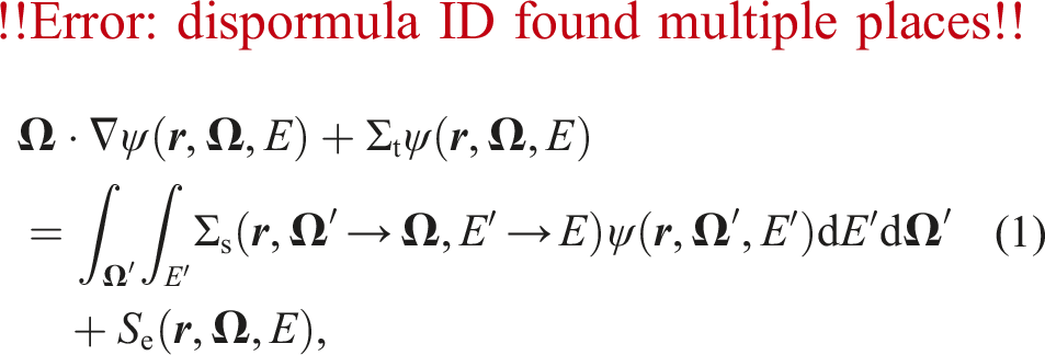
The first-order form of the time-independent BTE is given by
We give a summary of our sub-grid scale FEM discretisation below, for more details please see Hughes et al. (1998, 2006); Candy (2008); Buchan et al. (2010). A sub-grid scale discretisation decomposes the solution as
We replace 1. Solving for the stabilised continuous solution 2. Solving for the discontinuous correction 3. Combining the (interpolated) continuous solution and the discontinuous correction:
Steps 2 and 3 are trivial. For Step 1 in problems without scattering, we can build an assembled version of
3. Reduction multigrid
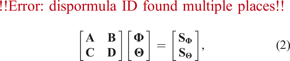
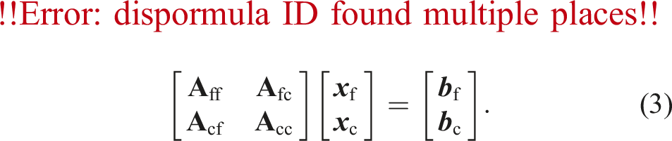
Reduction multigrids are formed with a coarse/fine (CF) splitting of the unknowns. If we consider a general linear system
Ideal prolongation and restriction operators are given by
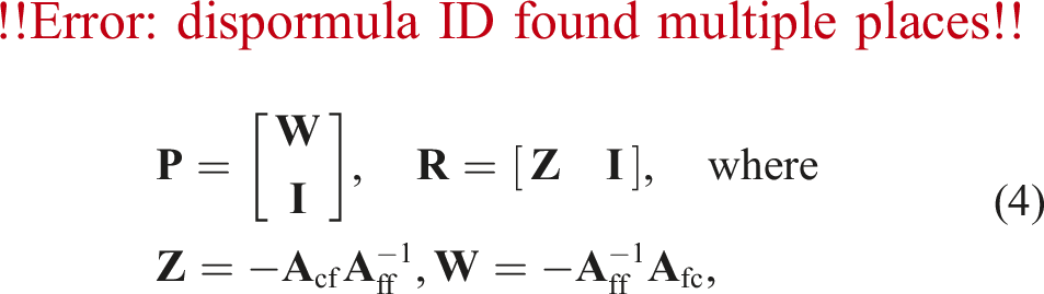
The approach we describe below computes an approximation,
3.1. AIRG
Approximate ideal restriction with GMRES polynomials (AIRG) uses fixed-order GMRES polynomials to compute
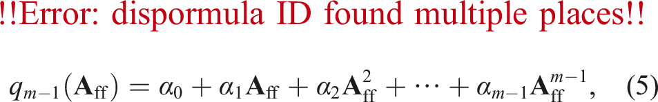
We found in Dargaville et al. (2024a) that low-order polynomials (m ≈ 3) were sufficient to give good results with our multigrid, and hence we can use a communication-avoiding algorithm (by orthogonalising the power-basis in a single step) to compute the coefficients. We then explicitly built an an assembled matrix representation of our polynomial, with a matrix-matrix product used to compute our approximate ideal operators. We also used this assembled matrix as our F-point smoother during the solve; the stationary polynomials could alternatively be applied matrix-free if desired. In this work we only use assembled versions of our polynomials.
In Dargaville et al. (2024a) we found this was a very effective approach for generating
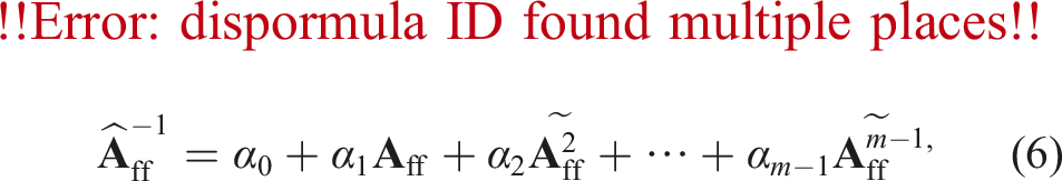
In this work we have instead written a fast method to compute the sum of fixed-sparsity powers of arbitrary order. We refer to enforcing the sparsity of
In summary, the setup of our AIRG multigrid requires on each level: 1. CF splitting 2. Extraction of required submatrices, for example, 3. Generation of a normally distributed rhs (with a Box-Muller transform), 4. m matvecs to compute the power basis, 5. QR decomposition of 6. Solution of the least-squares system 7. Calculation of matrix powers of 8. Building an assembled version of 9. Matrix-matrix product for the restrictor in (4), 10. Equivalent calculation for the prolongator or the generation of a classical one-point prolongator 11. Matrix-triple-product,
In the following section we describe the CF splitting algorithm that has been specifically tailored for parallel reduction multigrids.
4. CF splitting
Classical multigrid coarsening algorithms (e.g., Ruge-Stuben) rely on heuristics to produce CF splittings that result in good grid transfer operators and small, sparse coarse grids (see Alber and Olson (2007) for a review). Ruge-Stuben coarsening for example uses:
The heuristic
For AIRG, we only require that
MacLachlan and Saad (2007b,a) produced CF splitting algorithms specifically designed to give diagonally dominant
We take inspiration from those works and seek a highly parallel CF splitting algorithm that produces a diagonally dominant
Enforcing
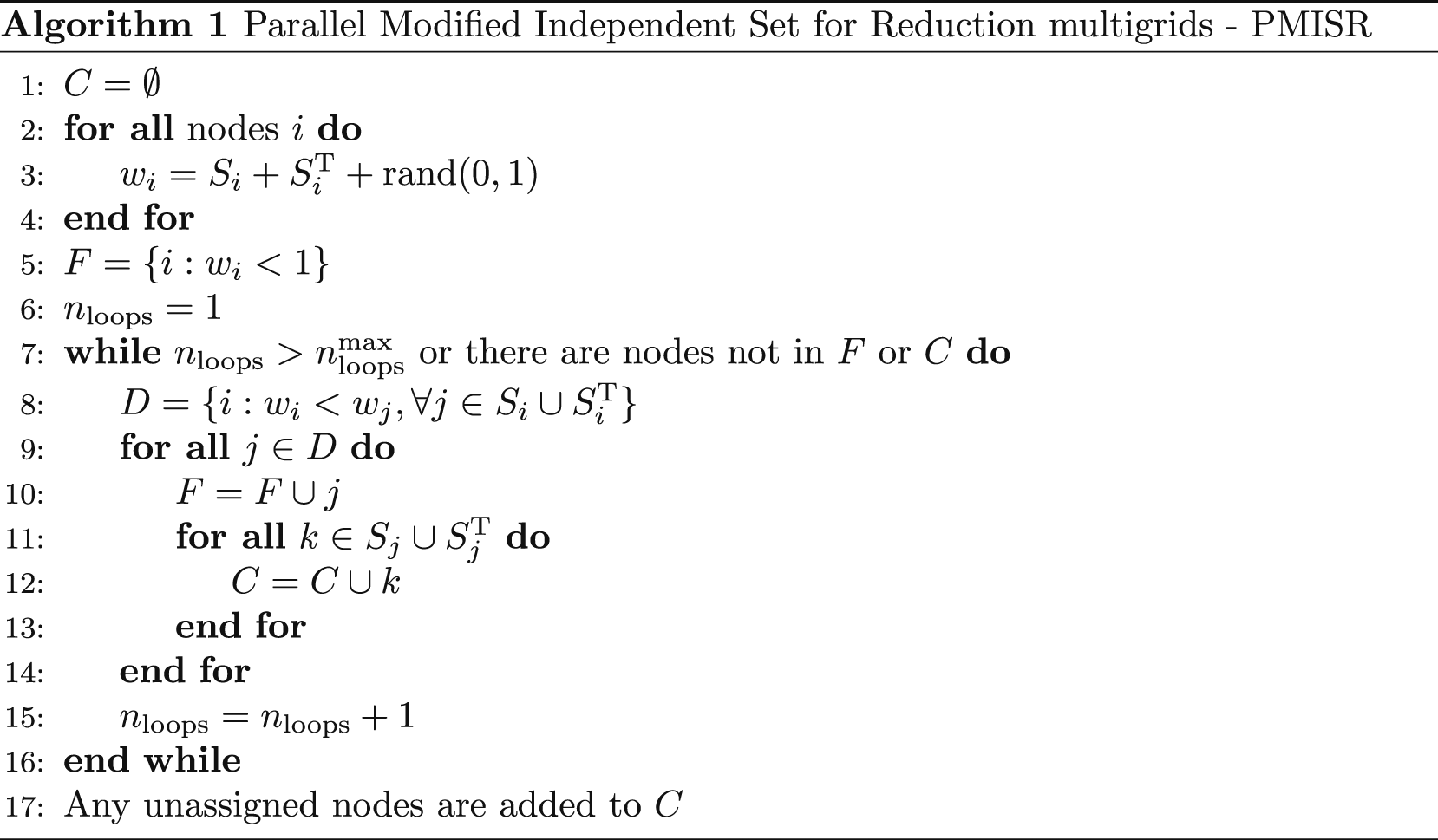
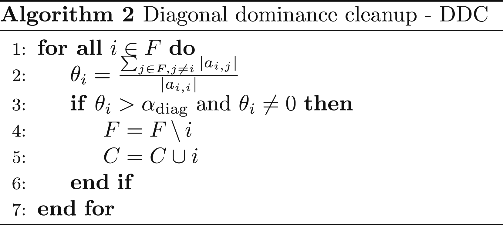
After a first pass with Algorithm 1, we perform a second pass with Algorithm 2 in order to weakly enforce
In summary, our CF splitting algorithm is one pass of PMISR followed by one pass of DDC. We have two parameters, α the strength parameter and αdiag the maximum row-wise diagonal dominance ratio. Choosing αdiag < 1.0 enforces strict diagonal dominance. We have found that rather than choosing αdiag directly, choosing αdiag such that a constant fraction of the least diagonally dominant F-points are converted to C-points performs well across a range of problems. The αdiag that gives this constant fraction can be calculated quickly by using the QuickSelect algorithm, or an approximate αdiag can be calculated by binning the diagonal dominance ratios and choosing the closest bin boundary. We use this approach with 1000 bins.
5. Results
To illustrate the performance of our CF splitting and AIRG, we show results from a streaming problem in 2D (zero scatter and absorption cross-sections). Our test problem is a 3 × 3 box, with an isotropic source of strength 1 in a box of size 0.2 × 0.2 in the centre of the domain. We apply vacuum conditions on the boundaries and discretise with unstructured triangles and ensure that the grids we use in any weak scaling studies are not semi-structured (e.g., we don’t refine coarse grids by splitting elements). We use uniform level 1 refinement in angle, with 1 angle per octant (similar to S2). Our matrix is therefore block diagonal, where each angle block is a stabilised CG discretisation of a time-independent advection equation, where the direction of the velocity is given by the angular direction. We do not exploit the block structure in this work; we apply the CF splitting and AIRG directly to the entire matrix.
In the results below, we apply AIRG as a solver with an undamped Richardson with a relative tolerance of 1 × 10⁻¹⁰ and zero initial guess. We solve
The code for AIRG and the PMISR DDC CF splitting is available in the open-source
5.1. Serial comparison
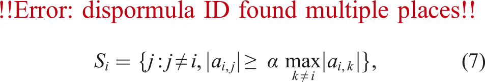
In this section we show the results from a single unstructured spatial mesh to give some insight into the behaviour of our CF splitting algorithm, before moving into parallel. We use the same parameters for AIRG as in Dargaville et al. (2024a); we should note, however, in this work that we use the SoC defined in (7) with absolute values, so our results are not identical even when using the same CF splitting algorithm. To approximate
Figure 1 shows a histogram of the diagonal dominance ratios for each row of Row-wise diagonal dominance of 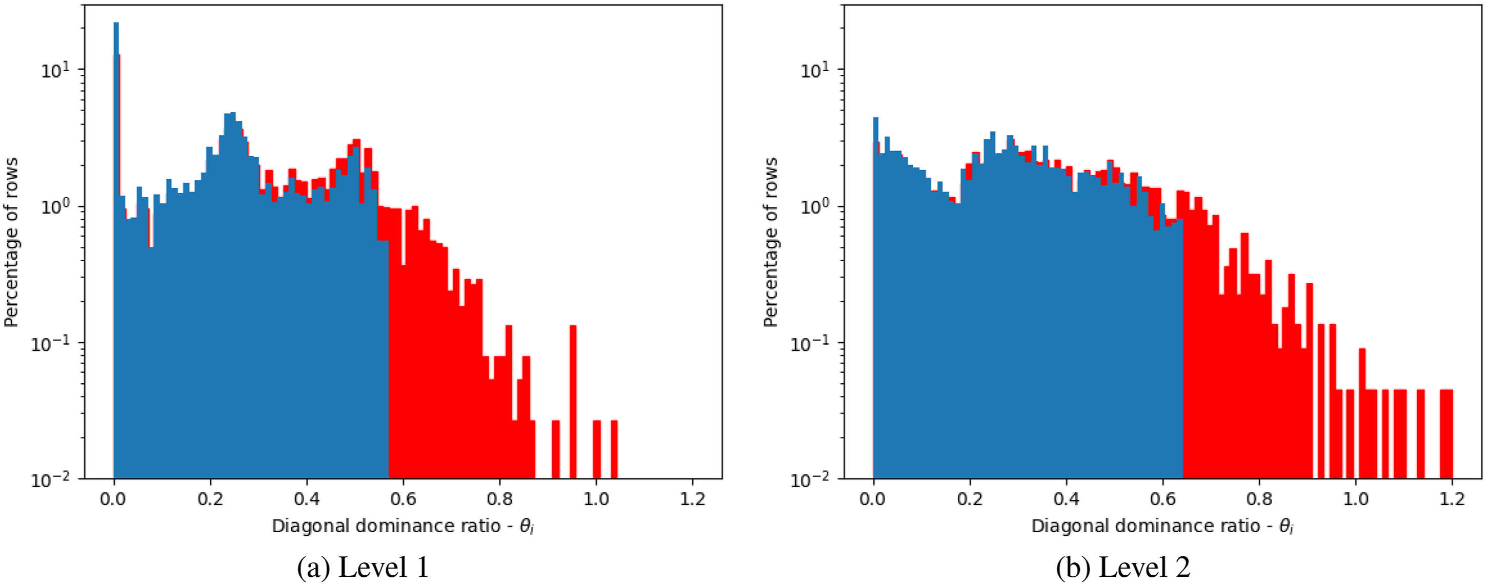
Figure 2 shows the resulting C and F points on the top grid, for two different angles. We can see in both Figures 2(a) and (b) that a semi-coarsening is produced, with the F-points aligned (roughly) perpendicular to the angular direction (i.e., the “flow”), as might be expected. Only weak off-diagonal entries should therefore be present in CF splitting produced by PMISR DDC on the top grid with strong tolerance 0.5 on an unstructured mesh with 2313 nodes. White squares are C-points, blue squares are F points. The red squares are C-points that were converted from F-points by the second pass with DDC with fraction of 10%. (a) Angle 1 - direction (1,1), (b) Angle 2 - direction (−1, 1).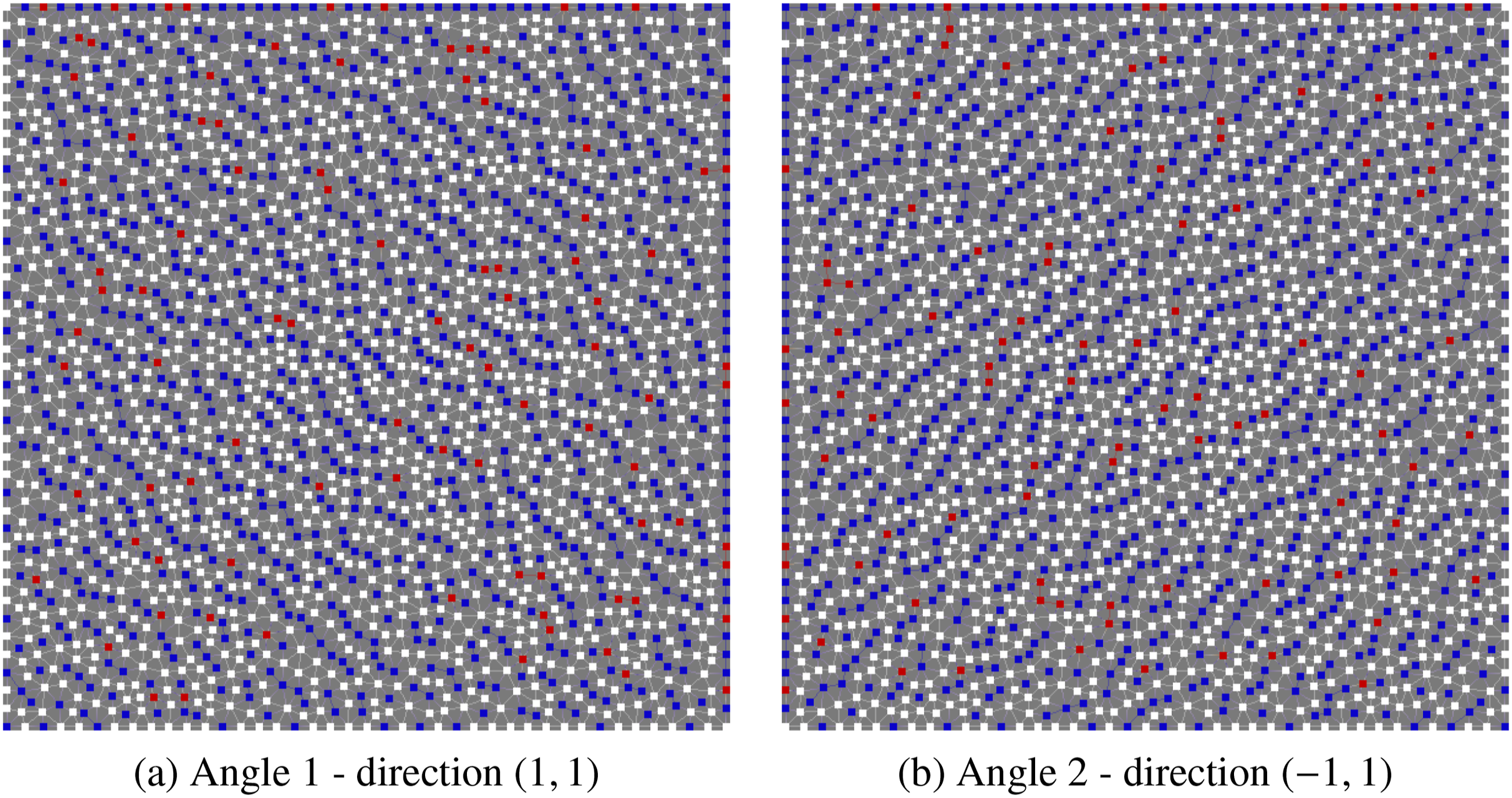
5.1.1. Strong tolerances
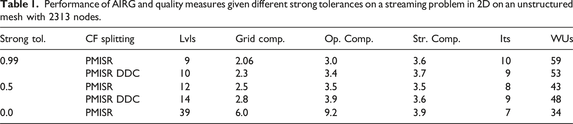
Performance of AIRG and quality measures given different strong tolerances on a streaming problem in 2D on an unstructured mesh with 2313 nodes.
We also measure the “storage complexity”, which reflects the relative storage required to perform a solve. With only up F-point smoothing we do not need to store the full matrix on each level once the next coarse matrix is produced in the setup, we only require 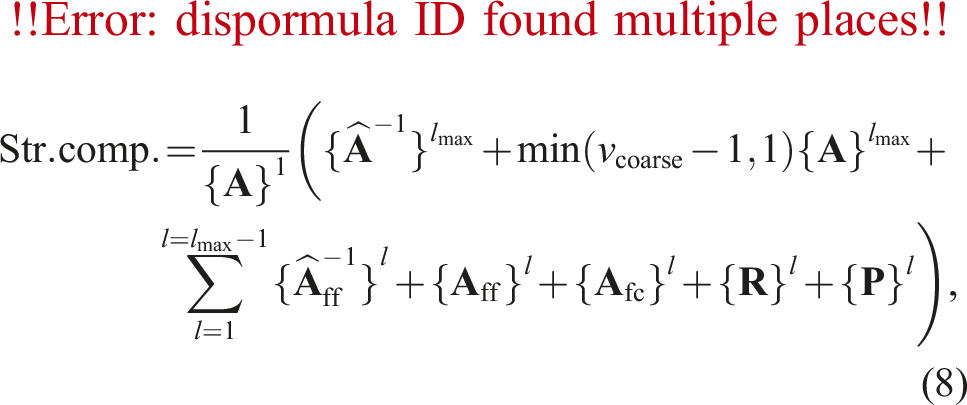
Table 1 shows that with a strong tolerance of 0.99 and one pass of PMISR, we achieve a grid complexity of 2.06. In advection problems (or a uniform angle discretisations of Boltzmann problems in the streaming limit), if we wish to avoid strong connections in CF splitting produced for angle 1 (direction (1,1)) by PMISR DDC on the top grid of an unstructured mesh with 2313 nodes. White squares are C-points, blue squares are F points. The red squares are C-points that were converted from F-points by the second pass with DDC with fraction of 10%. (a) Strong tolerance 0.99, (b) Strong tolerance 0.0.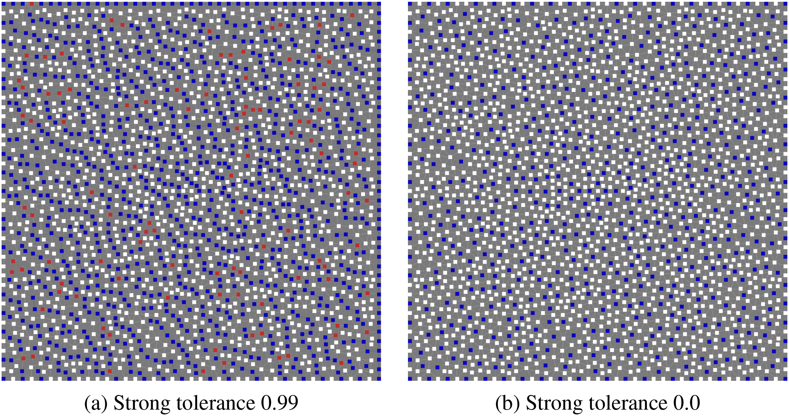
We can see that decreasing the strong tolerance to 0.5, either with or without a second pass of DDC, produces a slower coarsening but also results in less work units compared to a tolerance of 0.99. In this case, the second pass of DDC has increased the number of WUs compared to a single pass of PMISR. As might be expected, DDC can “cleanup” a poor CF splitting and improve convergence, but if the CF splitting is good a second pass of DDC will slow down the coarsening without much benefit. In both the 0.99 and 0.5 case, the operator complexity and storage complexity are very similar as might be expected.
Moving to the strong tolerance of 0.0, on the top grid this gives a maximal independent set in the connectivity of the spatial mesh for each angle, as the symmetrized strong connections with a strong tolerance of 0.0 is simply the adjacency graph of the matrix; see Figure 3(b). The benefit of producing an independent set in the adjacency graph of the matrix is that
We can see, however, that although the operator complexity is 9.2, this is not a good surrogate for the memory required during the solve, as the storage complexity is 3.9. This is only slightly higher than with the two other tolerances. We see that an independent set coarsening actually gives a method with the best convergence, with only 7 iterations and 34 WUs. We should note we only perform one up F-point smooth with a (diagonal) fixed-sparsity GMRES polynomial as
One of the benefits of an independent set CF splitting for Boltzmann transport problems is that with a uniform angle discretisation, the block structure in angle means that an independent set in the adjacency graph of the matrix is independent of angle (ignoring the boundary conditions). This allows even greater re-use of the CF splitting and symbolic matrix-matrix products than relying on angular symmetry as mentioned above (again dependent on drop tolerances/padded sparsity) and despite the greater number of levels this may lead to low setup times.
5.1.2. Serial comparison of CF splitting algorithms
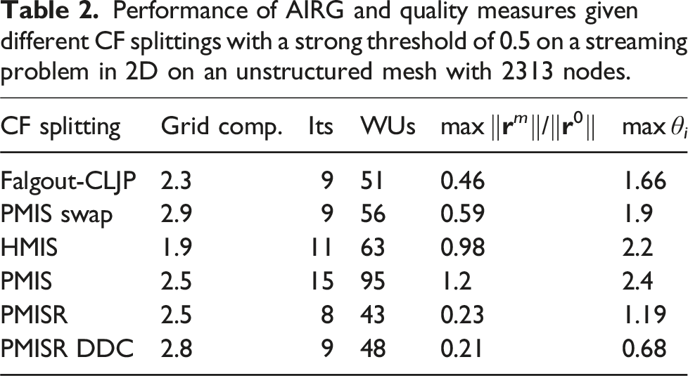
Performance of AIRG and quality measures given different CF splittings with a strong threshold of 0.5 on a streaming problem in 2D on an unstructured mesh with 2313 nodes.
In this section we also show the maximum diagonal dominance ratio θ
i
, for each row of
Condition number on each level given different CF splittings with a strong threshold of 0.5 on a streaming problem in 2D on an unstructured mesh with 2313 nodes.
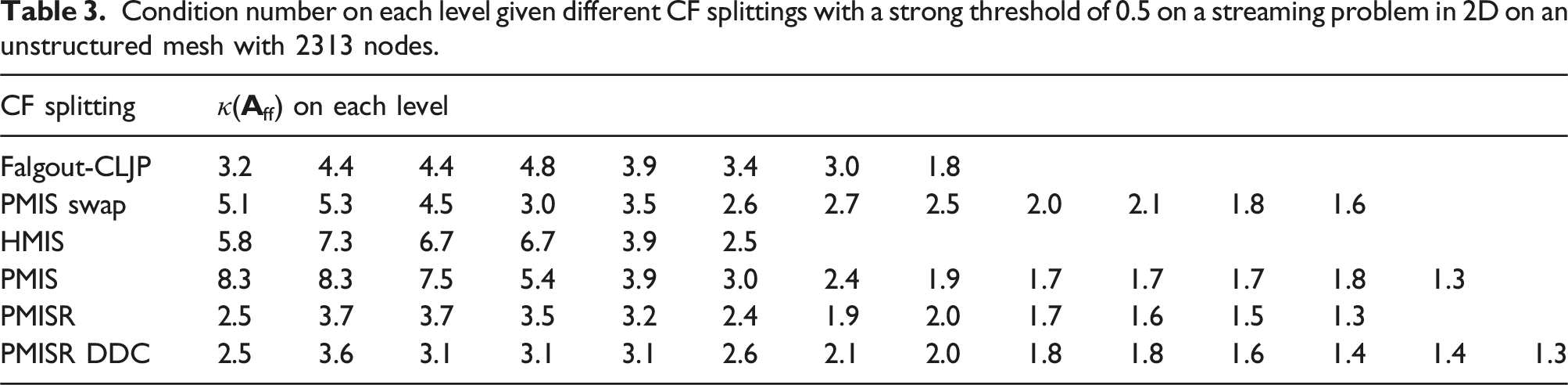
Furthermore Table 2 shows our PMISR CF splitting (without a second pass of DDC) performs the best out of all the CF splitting algorithms tested; the improved performance compared to PMIS swap shows that the two methods are not equivalent and hence it is worth ensuring each F-point has the smallest measure. The worst-case GMRES bound across the hierarchy with PMISR is roughly half that of the Falgout-CLJP method. We see that applying PMISR followed by a second pass of DDC with a 10% fraction almost halves the worst diagonal dominance ratio, while only slightly decreasing the worst-case GMRES bound. In practice our GMRES polynomials are very strong approximations and we find they are less sensitive to the diagonal dominance ratio than say a Jacobi method. Overall we find either PMISR or PMISR DDC produce the best CF splittings, with the lowest condition numbers, diagonal dominance ratios and worst-case GMRES bounds. On more refined spatial meshes, typically we find that PMISR DDC performs the best. We now move to parallel results.
5.2. Parallel results
We now investigate the parallel performance of our CF splitting algorithm and AIRG multigrid. We show strong and weak scaling results in parallel on ARCHER2, a HPE Cray EX supercomputer with 2 × AMD EPYC 7742 64-core processors per node (128 cores per node). All timing results are taken from compiling our code, PETSc 3.14 and hypre with “-O3” optimisation flag. Our goal in this section is to achieve the smallest solve time, as we can amortize the setup cost over many solves in multi-group Boltzmann problems. Given this, we searched the parameter space to try and find the best values for drop tolerances, strength of connections, etc, although more optimal values may be possible.
Both Algorithms 1 & 2 are very parallel and suitable for GPUs. We can introduce two further modifications to improve the parallel performance. In PMISR we avoid the reduction at each iteration which computes the global number of unassigned nodes in Line 7 of Algorithm 1. Instead we allow the specification of a maximum number of iterations with
In the results below, unless otherwise noted we use one pass of PMISR with a strong tolerance of 0.5 and
5.2.1. GMRES polynomial order
Time to compute and build assembled versions of GMRES polynomials across all levels on 8 nodes (1024 cores) of ARCHER2. The shaded rows represent fixed-sparsity GMRES polynomials (polynomial order
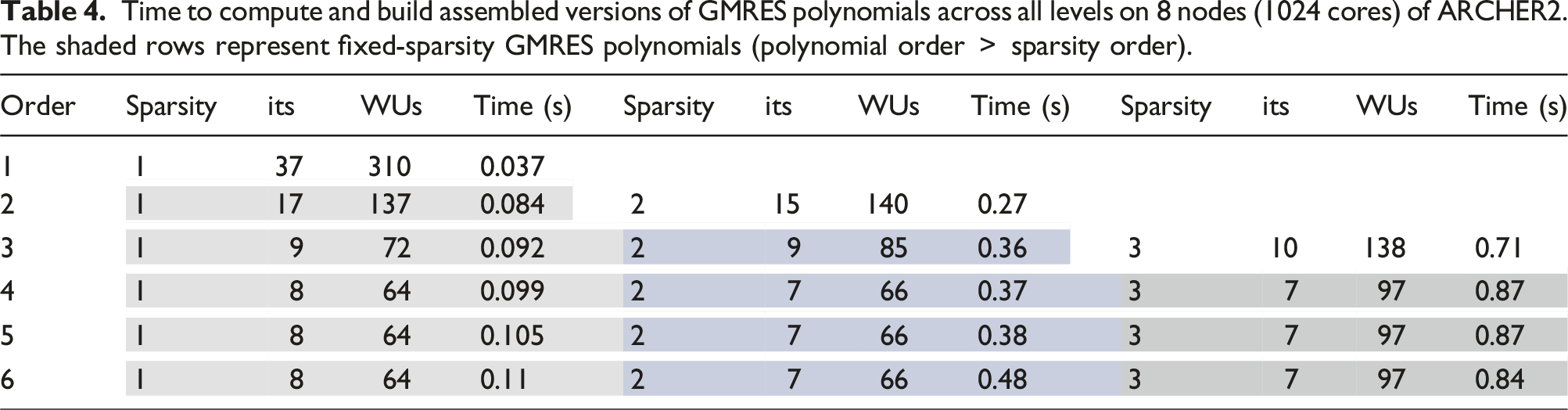
We can see that as expected, the higher the order of the GMRES polynomial used, the more expensive it is to setup, but the better the convergence in the resulting multigrid. Moving from first order to third decreases the iteration count from 37 to 10, but the cost increases by approximately 19×. Table 4 shows that the fixed-sparsity polynomials (i.e., sparsity
5.2.2. Optimisations for parallel multigrid
Before we investigate the strong and weak scaling, we first discuss commonly used methods to improve the performance of multigrid methods in parallel. May et al. (2016) discussed three main strategies, namely: truncating the multigrid hierarchy, allowing a subset of MPI ranks to have zero unknowns and agglomerating unknowns onto a new MPI communicator with fewer MPI ranks. These can be used with topology aware communication strategies in the matrix-vector and/or matrix-matrix products (Bhatele and Kale, 2008; Bienz et al., 2019, 2020) along with repartitioned coarse grids (Adams et al., 2004; Alef, 1991).
Increasingly non-local operators can change the balance of work to communication on the coarse grids, while the natural difference in coarsening rates on different ranks with unstructured grids can alter the load balance. Repartitioning can manage both these trends, while also either retaining or decreasing the number of active MPI ranks. The repartitioning can be simple (e.g., odd ranks send their data to even ranks) or mesh partitioning software like ParMETIS (Karypis and Kumar, 1995) can be used to balance the work and communication over any number of active ranks.
Figure 4 shows that without repartitioning, in a test with 18M elements and 9M CG nodes on 32 nodes of ARCHER2, our slow coarsening means we have around 30 levels in our hierarchy. We also see that the ratio of local to nonlocal work decreases as we coarsen, making our lower levels communication bound. We found this average ratio of local to nonlocal nnzs a good metric to trigger repartitioning; achieving good performance with this parameter is machine dependent. On ARCHER2 we use a value of 2. We chose to reduce the number of MPI ranks by half when we trigger repartitioning as this matches the expected coarsening rate of around 1/2 (in both 2D and 3D). Average ratio of local to non-local nnzs across active MPI ranks on each level on 32 nodes (4096 cores) of ARCHER2. Black is with no repartitioning,  is with simple repartitioning,
  is with ParMETIS repartitioning onto fewer ranks.
Figure 4 also shows a comparison between repartitioning with ParMETIS and a “simple” repartition where we simply halve the number of active MPI ranks (e.g., rank 1 sends all of its unknowns to rank 0, rank 3 to rank 2, etc.). We can see that both ways of repartitioning ensure a local to nonlocal ratio above two throughout the hierarchy. The “simple” repartitioning is triggered 10 times, giving lower grids on a single active MPI rank (hence the disappearance in Figure 4 after level 23 as the work is entirely local). The ParMETIS repartitioning, however, is only triggered 5 times, as the minimisation of the edge cuts gives a significant improvement in the communication stencil required and hence the average local to nonlocal ratio; this is particularly visible after the first repartition on level 6.
We could allow the repartitioning with ParMETIS to occur independently from the decrease in the number of active MPI ranks; for example, GAMG in PETSc allows the repartioning of every coarse grid, with the number of active MPI ranks only decreasing where necessary to ensure each local coarse grid has a set number of unknowns (the default is 50). We found combining these reduced the number of times we repartition, decreasing setup times without any large effect on solve times; on 32 nodes for example, we found repartioning every coarse level with ParMETIS and only decreasing the number of active ranks when the local to nonlocal nnzs ratio hit 2 actually increased our solve time by around 2%–5%. This is because of the extra communication introduced into the grid-transfer operators between levels when repartitioning has occurred.
We use an “interlaced” repartitioning as we find this performs best, for example, if our MPI rank numbering increases with the node number and the number of active MPI ranks is halved, each node has half the active number of ranks, rather than half the number of nodes being full. This also helps decrease the peak memory use on any given node. Furthermore, an interlaced repartition leaves idle cores on each node which allows the use of shared memory parallelism with OpenMP on lower levels. We experimented with this and found we could achieve good speedups in many aspects of the setup, particularly the assembly of the fixed-sparsity GMRES polynomials (Point 8 in Section 3.1). The matrix-matrix products used to form the restrictors and coarse matrices, however, did not see much speedup, as the use of drop tolerances in our hierarchy mean our matrices rarely become dense enough in the streaming limit; we found we required >30 nnzs per row to see good speedups. We did not explore the use of OpenMP parallelism during the solve on lower levels after repartioning, as it was difficult to implement the required non-busy MPI waits within the matrix-vector products used. We believe this would be worth exploring in the future, as the repartioning means the lower grid matrix-vector products potentially have enough local rows to see good speedups. We should note that none of the results in this paper use OpenMP in either the setup or the solve.
5.2.3. Timing results for parallel optimisations
Below we show results timing the solve and setup from the test problem in the previous section on 32 nodes. We examine a combination of the strategies listed above, namely no repartitioning, “simple” and ParMETIS repartitioning and the use of the node-aware matrix-vector and matrix-matrix products from the Raptor library (Bienz et al., 2020; Bienz and Olson, 2017). We compare the use of two different sparse matrix-vector (SpMV) routines used on every level as part of the smoothing, grid-transfer operators and coarse grid solve; namely the PETSc and the Raptor SpMVs. Similarly we tested using the PETSc, hypre and Raptor sparse matrix-matrix product (SpGEMMs) when computing the approximate ideal restrictor and the coarse grid matrices on every level. We found the hypre SpGEMM was more expensive than both the PETSc and Raptor SpGEMMs and hence we don’t show those results. The coarse grid matrix is computed with two SpGEMMs, that is,
Figure 5 shows timings for each component of our multigrid setup, as listed in Section 3.1. In this figure and the remainder of the paper, we split the cost of computing our approximate ideal restrictor into two parts: the cost of computing and assembling the GMRES polynomial (points 3–8 in Section 3.1) and the cost of the SpGEMM (point 9 in Section 3.1). Time taken for each component of the multigrid setup on each level on 32 nodes (4096 cores) of ARCHER2. The × is the CF splitting, the  is the prolongator, the
  is the GMRES polynomial, the + is the SpGEMM for the restrictor, the o is the SpGEMM for the coarse grid, the
  is the matrix extract and the
  is the repartitioning. (a) No repartition, PETSc SpMV & SpGEMM. Total setup: 42s, total solve: 0.26s. (b) No repartition, Raptor SpMV & SpGEMM. Total setup: 7.8s, total solve: 0.20s. (c) Simple repartition onto fewer ranks, PETSc SpMV & SpGEMM. Total setup: 15.1s, total solve: 0.33s. (d) ParMETIS Repartition onto fewer ranks. Raptor SpMV & SpGEMM. Total setup: 12.1s, total solve: 0.2s. (e) ParMETIS Repartition onto fewer ranks, PETSc SpMV & SpGEMM. Total setup: 13.0s, total solve: 0.086s.
We can see in Figure 5(a) that with no repartitioning, the SpGEMMs associated with our restrictor and the calculation of the coarse grid matrix are very expensive, particularly in the middle of the hierarchy where we are communication bound; the total setup time is 42 seconds, with the solve time 0.26 seconds. With no repartitioning, Figure 5(b) shows, however, that using the Raptor SpGEMM is significantly faster in the middle of the hierarchy. This gives a total setup time of 7.8s and a smaller solve time with the Raptor SpMVs of 0.2 seconds.
The simple repartitioning shown in Figure 5(c) also decreases the cost of the SpGEMMs significantly, while increasing the cost of computing both the GMRES polynomial and the CF splitting. This is because by increasing the local to non-local ratio, the simple repartitioning also increases the number of local rows and the cost of both the GMRES polynomial and CF splitting are closely tied to the local nnzs. We still find overall a significant decrease in setup time, at 15.1 seconds. The solve time, however, increases to 0.33 seconds. This is due to several effects: the increased number of local rows on active ranks after repartitioning, the increased communication required by the grid-transfer operators each time we hit a level that has been repartitioned (which happens 10 times with the simple repartitioning), along with the lack of optimisation of that communication.
The combination of repartitioning with ParMETIS and using Raptor gives a reduced setup cost, at 12.1s; this is largely due to (roughly) halving the time required by the SpGEMM for the restrictor, as the time to compute the coarse matrix was approximately the same. The biggest expense in the setup is now the repartioning with ParMETIS, taking a total of 8.9 seconds compared with 3.6 seconds with the simple method; the solve time is at 0.2s. Figure 5(e) shows that using ParMETIS repartioning but without Raptor, we have a slight increase in setup time at 13.0 seconds, but importantly the solve time has decreased to 0.086 seconds, which is the lowest value and 3× less than with no repartioning.
In order to further examine the impact of repartitioning and node-aware communication on the solve time, Figure 6 shows the time spent in F-point smoothing in the solve across the hierarchy; the time spent in SpMVs for the grid-transfer operators behaves similarly. We can see that without repartionining and using the PETSc SpMV, we have a significant increase in smooth time in the middle of the hierarchy, much like with the PETSc SpGEMMs discussed above. We can also see that the Raptor SpMV reduces this cost in the middle of the hierarchy; it is this effect that lead to the reduced solve time reported in Figure 5(b). Once repartitioning with ParMETIS has been enabled, however, we find that the Raptor SpMV can be more expensive on lower levels than the PETSc SpMV. We also compared the NAP-2 and NAP-3 communication options in Raptor but could not find settings that reduced the Raptor SpMV time below that of the PETSc SpMV when repartitioning was enabled. This is perhaps to be expected; node-aware communication is most beneficial when the communication volume is poorly optimised. Time spent in the F-point smooth on each level on 32 nodes (4096 cores) of ARCHER2. ● are with no repartitioning,  are with ParMETIS repartitioning onto fewer ranks. The solid lines are the PETSc SpMV, the dotted are the Raptor SpMV.
Hence we conclude that repartitioning with ParMETIS is crucial to the performance of both the solve and setup. In the setup of this test problem, we found that the Raptor SpGEMMs was sometimes the cheapest. If we chose not to repartition, using the Raptor SpGEMM significantly reduced the setup time, giving the lowest value. If we repartition with ParMETIS, however, the Raptor SpGEMM was cheaper for some levels/operators and not others. We also found this in other problems when strong/weak scaling; the Raptor SpGEMM ranged from twice to half the cost of the PETSc SpGEMM when ParMETIS repartitioning was used. In the solve, we find it is only worth using the Raptor SpMV if we have not repartitioned with ParMETIS; the lowest solve time comes from repartitioning with ParMETIS and using the PETSc SpMVs. Given this, we would only recommend using the node-aware SpMV and SpGEMM from the Raptor if the coarse grids have not been repartitioned onto fewer MPI ranks with an optimising library such as ParMETIS.
We can further improve the setup and solve time by truncating our multigrid hierarchy, but this requires a strong coarse solver. We found using an exact LU factorisation was far too expensive and resulted in poor scaling, in both the setup and solve phase. Instead we use our GMRES polynomials as an iterative coarse grid solver, truncating the hierarchy when the coarse grid has approximately 300k unknowns. We use three iterations of a 12th order GMRES polynomial with first order fixed sparsity. We also investigated using a 12th order GMRES polynomial applied matrix free (i.e., without first order fixed sparsity), but we found it faster to apply several iterations of the fixed-sparsity polynomial (at the cost of storing an assembled approximate inverse with fixed sparsity).
The GMRES polynomial is very cheap to setup when used a coarse grid solver. For the example in Figure 5(e), truncating to 14 levels results in a cumulative GMRES polynomial setup time of 0.14s on levels 1–13 with the coarse level setup on level 14 costing just 0.03s. In the remainder of this paper, unless otherwise noted we truncate our hierarchy and use a GMRES polynomial as the coarse grid solver, use the PETSc SpMV and SpGEMM and also repartition our coarse grids with ParMETIS and half the number of active MPI ranks when the local to non-local nnzs ratio hits 2.
5.2.4. Strong scaling
Strong scaling of AIRG with ParMETIS repartitioning onto fewer ranks and a truncated hierarchy (13 levels) on ARCHER2, on a test problem with 4.5 M elements and 2.3 M CG nodes and 4 angles. The solve takes 8 iterations with 64 WUs.
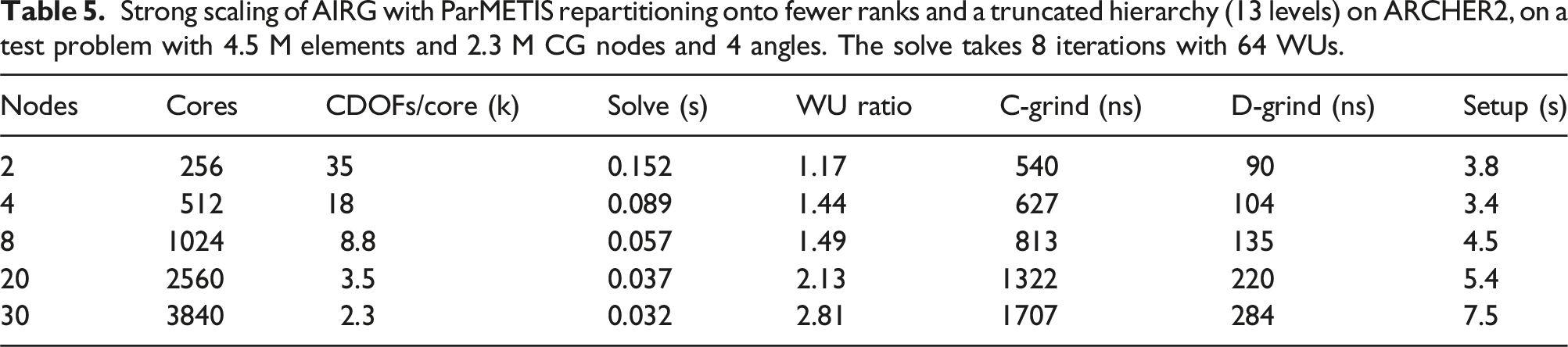
The “WU ratio” in Table 5 is the solve time divided by the WUs, scaled by the time to compute a top grid matvec. A value of 1 would indicate that the WUs in the solve perfectly predicts the observed solve time and hence there is no communication bottleneck on the lower grids. We can see that the WU ratio increases as we strong scale, up to 2.81 on 30 nodes. Similar to the setup, this is due to the increasing communication bottleneck on the lower grids. Again the repartitioning with ParMETIS helps keep this ratio low; without repartitioning on 30 nodes we have a WU ratio of 10.2.
Table 5 also includes two different ‘grind times”. This is the total solve time, divided by either the NCDOFs or the NDDOFs per core and divided by the iteration count. This gives the cost per V-cycle scaled by the number of continuous or discontinuous DOFs per core. In Dargaville et al. (2024a) we show good results from using a single V-cycle on the streaming/removal operator as a preconditioner in problems with scattering. Hence we show the grind times as they quantify the cost of a single V-cycle. We can see from the C-Grind time that our solve is most efficient with more unknowns per core. At approximately 35k CDOFs/core we require 540 ns per CDOF/core/V-cycle. If we compare this with the grind time of a structured grid DG-sweep code (which is the time required per DDOF/core/sweep), this seems expensive; high-performance structured grid DG-sweeps can achieve times as low as 30-100 ns. We should note, however, that the C-Grind time is that required to perform a V-cycle on a stabilised continuous discretisation, namely Step 1 in Section 2. Our discretisation is discontinuous, though it relies on computing the solution of a stabilised continuous problem first, with the further work required to then compute our discontinuous solution small and trivially parallelisable (Step 2 and 3 in Section 2).
Hence we also also compute the D-grind time, which shows the cost of solving our stabilised continuous problem but scaled by the number of discontinuous DOFs. This helps us make comparisons with DG-sweep codes; we achieve 90 ns per DDOF/core/V-cycle on an unstructured grid on ARCHER2. Of course a DG-sweep exactly inverts the streaming operator (ignoring the impact of cycles on unstructured grids), whereas the D-grind time is that for a single V-cycle, which only reduces the residual by roughly an order of magnitude. As we showed in Dargaville et al. (2024a), however, a single V-cycle is sufficient when the streaming/removal operator is used as a preconditioner. Using a single V-cycle as a preconditioner on the angular flux requires more memory in the solve when compared to the source iteration used in typical DG-sweep codes. When used with a stabilised continuous discretisation, however, the smaller number of DOFs helps reduce the required memory in the solve and results in grind times that are competitive with structured grid DG sweeps, even on unstructured grids.
5.2.5. Weak scaling
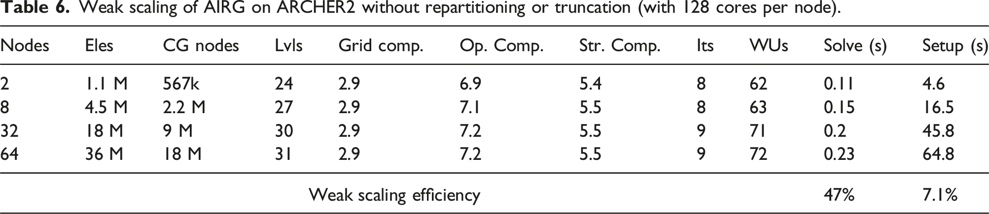
The previous section established that around 35k CDOFs per core with AIRG gives good performance. The mesh infrastructure we have built our implementation on has a strict limit on the number of elements we can use; in parallel this limits the weak scaling results we can show. Given this, we decided to decrease the number of DOFs per core in our weak scaling experiments. This is in an attempt to increase the communication bottlenecks which would happen naturally at higher core counts, despite mesh limitations preventing us from running with a higher number of cores. Hence in the experiments below we show results from only using around 8.8k CDOFs per core. Similarly, we only use 4 angles in our angular discretisation (uniform level 1 refinement) in order to reduce the amount of local work, again exposing communication bottlenecks.
Weak scaling of AIRG on ARCHER2 without repartitioning or truncation (with 128 cores per node).
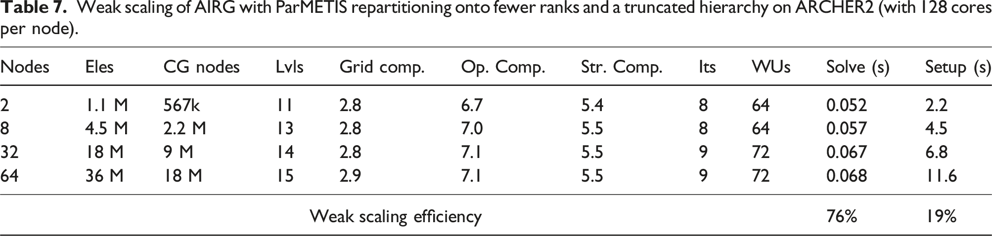
Weak scaling of AIRG with ParMETIS repartitioning onto fewer ranks and a truncated hierarchy on ARCHER2 (with 128 cores per node).
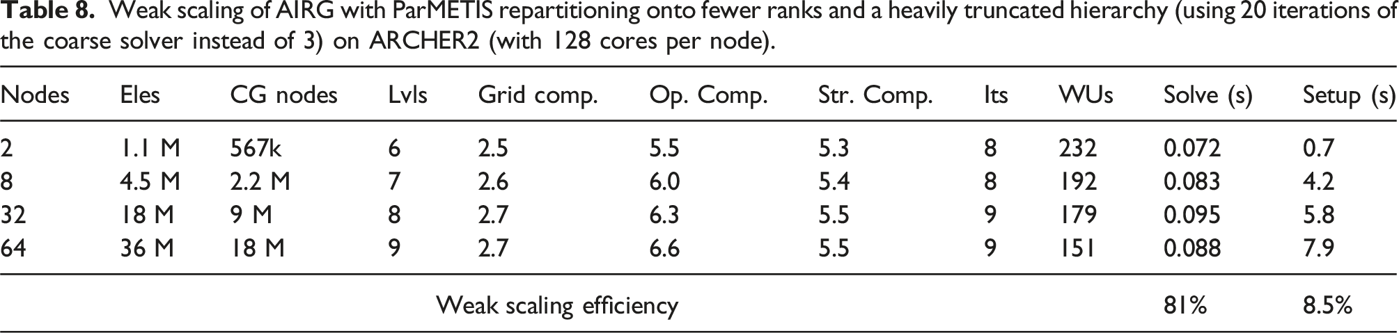
Weak scaling of AIRG with ParMETIS repartitioning onto fewer ranks and a heavily truncated hierarchy (using 20 iterations of the coarse solver instead of 3) on ARCHER2 (with 128 cores per node).
5.2.6. Weak scaling with strong tolerance 0.0
Weak scaling of AIRG with strong tolerance 0.0 with ParMETIS repartitioning onto fewer ranks and a truncated hierarchy on ARCHER2 (with 128 cores per node).
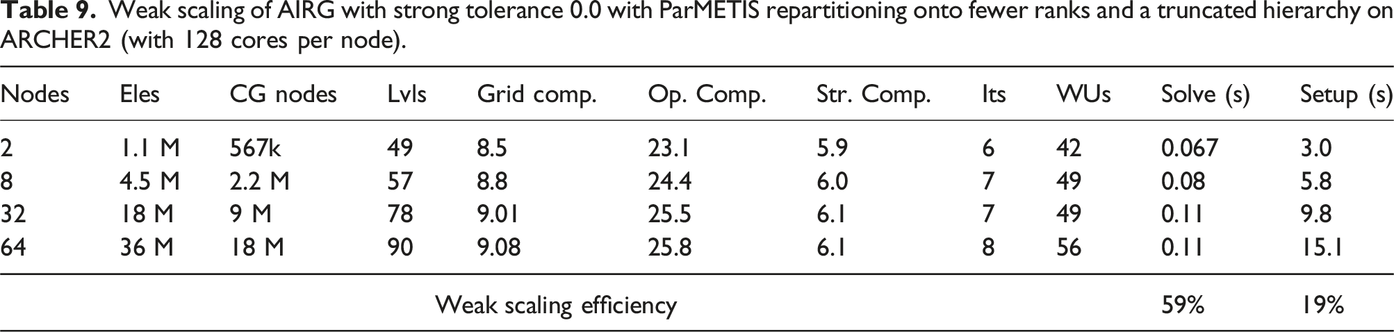
It is the combination of only F-point smoothing and the ParMETIS repartitioning that is responsible for such good performance despite the slow coarsening. The small number of F-points means only F-point smoothing is cheap and doesn’t require an expensive C-point residual or C-point smooth, giving a low number of WUs. Similarly the SpGEMMs required to compute the approximate ideal restrictor are very rectangular, with the SpGEMMs required to compute the coarse matrix benefiting from large identity blocks in
Using a strong tolerance of 0.0 and hence a diagonal
5.2.7. Parallel comparison of CF splitting algorithms
Similar to Section 5.1.2 we show a comparison between different CF splitting algorithms, but now in parallel. We compare weak scaling results for the hypre implementations of Falgout-CLJP, PMIS “swap” as defined in Section 5.1.2 and HMIS against PMISR and PMISR DDC with 10% local fraction. We don’t show results from PMIS as it performed very poorly. In all these tests we use a strong tolerance of 0.5.
Weak scaling of AIRG with different CF splitting algorithms with strong tolerance 0.5, no truncation and ParMETIS repartitioning onto fewer ranks on ARCHER2 (with 128 cores per node). The minimum times are shaded.
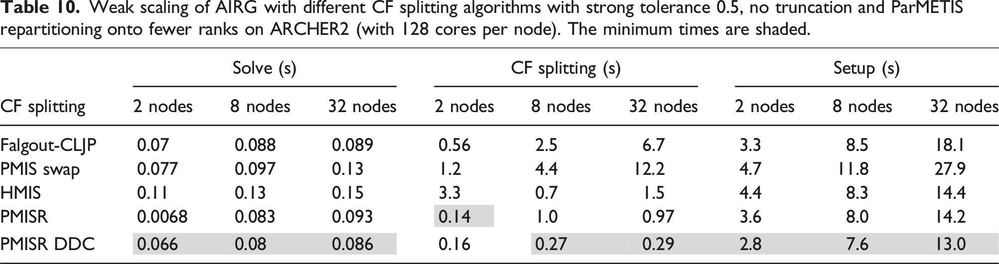
Of the hypre CF splitting algorithms, Table 10 shows that the Falgout-CLJP produces the best solve time, only 5% slower than that of PMISR DDC. The time required by PMISR DDC to compute the CF splitting, however, is much less; on 32 nodes it is 23× faster. This confirms that our PMISR DDC CF splitting algorithm is very performant in parallel and an excellent choice for use with reduction multigrids which require diagonally dominant
5.2.8. Weak scaling comparison with ℓAIR
To finish our weak scaling experiments, we compare our results with the hypre implementation of distance 2 ℓAIR. We tried to use parameters that gave the lowest solve time and best weak scaling in order to give a fair comparison with AIRG. We use 3 FCF-Jacobi up smooths, 5 damped Jacobi iterations as a coarse solver and a strong
hypre does not provide the ability to repartition coarse grids and hence the only technique we have to reduce the communication bottlenecks on lower grids in these hyperbolic problems is truncation. We attempted to use ℓAIR without truncating the hierarchy in order to compare against Table 6, but we found the setup was too expensive. Hence to begin, we truncated the hierarchy and used 12, 15, 18 and 21 levels, respectively. This resulted in 16 iterations in the solve and weak growth in the WUs with 316, 326, 331 and 333 WUs.
We should note it is difficult to compare the WUs between AIRG and the hypre implementation of ℓAIR as the cycle complexity output by hypre doesn’t include all the work associated with smoothing. In Dargaville et al. (2024a) we redefined the cycle complexity calculation in hypre to enable comparisons, but it is more difficult to deploy this modification on ARCHER2. As such, we only note the WUs for ℓAIR to make clear that the heavy growth in the solve time shown in Figure 7(a) is caused by communication bottlenecks, rather than growth in work. We can also see in Figure 7(a) that ℓAIR with truncation is more expensive in the solve than AIRG without truncation (or repartitioning); with 64 nodes AIRG is 1.8× faster. Comparison of weak scaling results for AIRG and  AIR on ARCHER2, from 2 nodes (256 cores) to 64 nodes (8196 cores) with 8.8k CDOFs/core. The solid
  is ℓAIR with a truncated hierarchy, the dotted
  is ℓAIR with a hevaily truncated hierarchy. The solid ● is AIRG with no truncation, the dashed ● is AIRG with ParMETIS repartitioning onto fewer ranks and a truncated hierarchy, the dotted ● is AIRG with ParMETIS repartitioning onto fewer ranks and a heavily truncated hierarchy. (a) Solve, (b) Setup.
The setup times for ℓAIR feature growth in the middle of the hierarchy, similar to that described in Section 5.2.2. With AIRG in the previous section, we found better performance from heavily truncated the hierarchy and increasing the number of iterations used in the coarse grid solve. Hence we investigated using 9, 10, 11 and 12 levels with 12 damped Jacobi iterations as a coarse solve with ℓAIR. Doing this introduced further growth in the iteration count, giving 18, 20, 21 and 21 iterations and 352, 398, 444 and 444 WUs. This resulted in a reduction of the solve times, despite the higher WUs, confirming the communication bottlenecks on the lower levels. We could not find a coarse grid solver that resulted in both flat iteration counts with this heavily truncated hierarchy and reasonable setup times in hypre. This helps show the strength of using a GMRES polynomial as a coarse grid solver in AIRG.
Figure 7(a) and (b) also show the results from Tables 7 and 8 which help demonstrate the impact of repartitioning with ParMETIS onto fewer ranks and truncation with AIRG. We see significantly lower setup and solve times. In particular, with a truncated hierarchy and ParMETIS repartitioning onto fewer ranks, the AIRG solve on 64 nodes is 5.9× faster than the ℓAIR implementation in hypre with a heavily truncated hierarchy.
6. Conclusions
In this work we examined the parallel scaling of the AIRG reduction multigrid when used to solve Boltzmann transport problems in the streaming limit on unstructured grids. The streaming limit gives a hyperbolic system and hence a semi-coarsening can be produced along the characteristics determined by the angular directions. This gives a coarsening rate of 1/2 (at best) and hence the multigrid hierarchy has many levels. Previously we found distance 2 approximate ideal interpolation gives good results in these problems (Dargaville et al., 2024a), although this long-range interpolation means our coarse grid matrices become increasingly non-local. These factors make the parallelisation of reduction multigrid for hyperbolic systems difficult.
To achieve good solve and setup times, we found it necessary to repartition our coarse grids onto fewer MPI ranks with ParMETIS and to truncate the multigrid hierarchy. We triggered the repartitioning when the local to non-local nnzs ratio decreased below a fixed threshold; on ARCHER2 we used a value of 2. We applied a GMRES polynomial as the coarse grid solve and found this was very cheap to setup, allowing heavy truncation without affecting the iteration count.
We introduced a two-pass CF splitting, denoted PMISR DDC, which was designed to give a diagonally dominant
When used with our sub-grid scale discretisation, strong scaling results on unstructured grids in 2D showed that using 35k CDOFs/core performed well in the solve with AIRG, though we found reductions in the wall time down to 2.3k CDOFs/core. Using 35k CDOFs/core, we found the grind time for a single V-cycle was as low as 90 ns per DDOF/core.
Our meshing software limited the weak scaling results we could show and hence we decided to decrease the CDOFs/core and use a low-order angular discretisation (i.e., very few DOFs/spatial node) in order to expose communication bottlenecks. When using 8.8k CDOFs/core, we found that the combination of our PMISR DDC CF splitting, ParMETIS repartitioning onto fewer ranks, truncating our multigrid hierarchy and using a GMRES polynomial as the coarse grid solver resulted in good weak scaling. Moving from 2 to 64 nodes, the iteration count increased from 8 to 9, with the number of work units increasing from 64 to 72. This gives a method that is very close to algorithmically scalable in the hyperbolic limit. The practical scaling in solve time we saw was very close to this ideal, with the time per iteration only increasing by 9.6%. This gave an overall weak scaling efficiency of 81% from 2 to 64 nodes on ARCHER2.
When compared to the ℓAIR implementation in hypre, we found that AIRG was faster and required less work units to solve. When we introduced ParMETIS repartitioning onto fewer ranks with AIRG and a truncated hierarchy, the solve time was 5.9× faster than with ℓAIR with heavy truncation. A large fraction of this speedup was due to the effect of repartitioning the coarse levels onto fewer MPI ranks, truncation of the hierarchy and the performant coarse grid solver. As such it could be worth introducing these techniques into the hypre implementation of ℓAIR. Typical elliptic multigrids can use aggressive coarsening to reduce the need for such techniques, but this is not available with reduction multigrids in hyperbolic systems, as the coarsening must be slow.
As with most algebraic multigrids, we found our setup time grew considerably. We observed a 5.2× increase in setup time from 2 to 64 nodes, though the overall time was less than the ℓAIR implementation in hypre. Again repartioning with ParMETIS was vital to ensuring the setup time remained low throughout the hierarchy. We also investigated using the node-aware matrix-vector and matrix-matrix products in the Raptor library. We found if no repartioning was performed the node-aware routines helped reduced the setup time considerably (while also decreasing the solve time), but if repartioning with ParMETIS onto fewer ranks was enabled it was often not worth using the node-aware routines.
The results from this paper show that it is now possible to achieve good weak scaling and fast solves for hyperbolic Boltzmann transport problems on unstructured grids, without the use of DG discretisations and sweeps. This allows different discretisation and solution methods to be used practically in transport at scale. The weak scaling results were generated with very few DOFs/core, which suggests that good scaling should be possible at higher core counts. Furthermore, the PMISR DDC CF splitting, matrix-vector and matrix-matrix products used are all well suited for use on GPUs. Many aspects of the (expensive) setup can also be re-used in Boltzmann problems, as typically we perform many solves in multi-group and/or eigenvalue problems. Future work will combine the use of our PMSIR DDC CF splitting and AIRG with the additive preconditioning method described in Dargaville et al. (2024a) in order to examine a parallel sweep-free method for solving Boltzmann problems with scattering.
Footnotes
Declaration of Conflicting Interests
The author(s) declared no potential conflicts of interest with respect to the research, authorship, and/or publication of this article.
Funding
The author(s) disclosed receipt of the following financial support for the research, authorship, and/or publication of this article: This work was supported by the Engineering and Physical Sciences Research Council; EP/T000414/1.
Note
Steven Dargaville is a researcher at Imperial College London, who works on building mathematical models and numerical methods for problems in the energy sector. This includes discretisation and iterative methods for Boltzmann problems that use current and emerging HPC platforms efficiently.
Richard Smedley-Stevenson is a Distinguished Scientist at AWE Nuclear Security Technologies which maintains the UK's nuclear deterrent capability and provides nuclear security advice to the UK government. He has over 35 years of experience at AWE developing physics simulation computer codes on high performance parallel computers, focussing on neutral particle transport models. He previously held a visiting professor position in the Applied Modelling and Computation Group (AMCG) at Imperial College London.
Paul Smith is the Technical Director of Amentum's ANSWERS Software Service which develops software for reactor physics, criticality, shielding and dosimetry applications. He has over 40 years experience in the nuclear industry. He is also a visiting professor in the Applied Modelling and Computation Group (AMCG) at Imperial College London and in the Nuclear Futures Institute at Bangor University.
Christopher Pain is a Professor in the department of Earth Science and Engineering at Imperial College London (ICL), UK. He is also head of the Applied Computation and Modelling Group (AMCG), which is the largest department research group at ICL and comprises of about 70 research active scientists. AMCG specialises in the development and application of innovative and world leading modelling techniques for earth, engineering and biomedical sciences. The group has core research interests in numerical methods for ocean, atmosphere and climate systems, engineering fluids including multiphase flows, neutral particle radiation transport, coupled fluids-solids modellingwith discrete element methods, turbulence modelling, inversion methods, imaging, and impact cratering.