Sage Journals: Discover world-class research

Abstract

We present a high-performance implementation of Seismic Redatuming by Inversion (SRI), which combines algebraic compression with mixed-precision (MP) computations. Seismic redatuming entails the repositioning of seismic data recorded at the surface of the Earth to a subsurface level closer to where reflections have originated. Marchenko-based redatuming is the best-in-class SRI method from a theoretical point of view because it can accurately handle full seismic wavefields with minimal data pre-processing. However, it requires intensive data movement, a large memory footprint, and extensive computations due to the need for manipulating large, formally dense, complex-valued frequency matrices in the bandwidth of the recorded seismic data. More precisely, at the heart of Marchenko modeling operator lies a Multi-Dimensional Convolution (MDC) operator, which requires the application of repeated complex-valued Matrix-Vector Multiplications (MVMs) with chosen set of seismic frequency matrices. SRI is deemed to be too time-consuming for realistic domain sizes and therefore industrially impractical. To alleviate these computational bottlenecks, we first improve the memory footprint of the MDC operator by using Tile Low-Rank Matrix-Vector Multiplications (TLR-MVMs); this exploits the low-rank nature of seismic recordings in the frequency domain, used as the kernel of the MDC modeling operator. MP computations are further introduced to increase the arithmetic intensity of the operators. We validate the numerical robustness of our synergistic approach on a benchmark 3D synthetic seismic dataset and demonstrate its use on various hardware architectures. We develop several FP32/FP16/INT8 MP TLR-MVM implementations with a limited and controllable impact on the overall accuracy of application. We achieve up to 63X memory footprint reduction and 12.5X performance speedup against the traditional dense MVM kernel on a single NVIDIA A100 GPU. Moreover, linear scalability is attained when deploying our implementation on eight A100 GPUs. Our implementations of the MDC operator integrate with the open-source PyLops framework for large-scale, matrix-free inverse problems.

Keywords

Mixed precision tile low-rank matrix-vector multiplication seismic redatuming

1. Introduction

Geophysical methods such as reflection seismology play a key role in the process of characterizing the Earth’s subsurface. In the past decades, these methods have been key enablers in the discovery and production of natural reserves (i.e., coal, oil, and gas). Nowadays, they are becoming valuable in the transition to a low-carbon future enabled by geothermal energy and carbon capture/storage, as recommended by the G20 report on reaching net-zero emissions IMF (2021). In recent years, very powerful inversion-based seismic processing algorithms have been developed by numerous researchers. Although they outperform the industry standard algorithms in terms of quality, their application to 3D field datasets remains a challenge, mostly due to the extreme computing requirements that these methods carry in terms of memory footprint and algorithmic complexity.

In particular, a novel family of methods has emerged under the name of Marchenko redatuming (Broggini et al., 2012); (Wapenaar et al., 2014); (Ravasi et al., 2016). Seismic redatuming consists of repositioning seismic data recorded at the surface of the Earth to a subsurface level closer to where reflections have originated. Marchenko-based redatuming can achieve such an objective using the full seismic wavefield with minimal pre-processing; however, this comes at the cost of intensive data movement, a large memory footprint, and extensive computations due to the need for manipulating large, dense matrices for a significant number of temporal frequencies. This stems from the fact that at the heart of the Marchenko modeling operator lies a Multi-Dimensional Convolution (MDC) operation, which necessitates performing repeated Matrix-Vector Multiplications (MVMs) with different seismic frequency matrices. As this operator corresponds to the most time-consuming aspect of the redatuming method presented in this work, and similar algorithms present in the geophysical (Van Groenestijn and Verschuur, 2009); (Amundsen, 2001); (Lopez and Verschuur, 2015) and ultrasound (Li et al., 2021) processing arsenals also rely on this operator, the development of faster and less memory demanding engines is of great interest to the scientific community.

In this work, we democratize Seismic Redatuming by Inversion (SRI) in the context of the Marchenko equations. We first propose to apply algebraic compression on the seismic frequency matrices to reduce their memory footprint; this in turn lowers the time to solution of the MDC operator using Tile Low-Rank (TLR) matrix approximations for the subsequent MVM operations. More precisely, TLR compression performs a singular value decomposition for each tile of the matrix of interest and retains only the most significant information up to an application-appropriate accuracy threshold. Whilst compressing the original seismic frequency matrices provides a significant size reduction, we show that this can be further reduced by applying a distance-aware matrix reordering technique prior to compression. Using Hilbert space-filling curves, we agglomerate nearby sources (and receivers), which correspond to the rows and columns of each frequency matrix, before tiling and compression, and eventually engender a better compression rate. Next, we introduce a novel Mixed-Precision (MP) algorithm to further increase the arithmetic intensity of Tile Low-Rank Matrix-Vector Multiplications (TLR-MVMs) by accumulating in high precision, while loading/storing data in low precision into/from registers. This improves the overall throughput of SRI. This combination of MP with TLR-MVMs is the critical synergism of our approach to SRI. It has also recently been employed on covariance matrices in a geospatial statistics application Gordon Bell Finalist paper (Cao et al., 2022).

The numerical robustness of the proposed approach is tested on a non-proprietary benchmark synthetic seismic dataset that is designed to be realistic both in terms of data size as well as field-related mathematical properties. Similarly, the portability of our implementation is showcased by deploying it on several hardware architectures, for example, Intel x86, ARM A64FX, NEC Vector Engine, and AMD and NVIDIA GPU systems, in each case leveraging the most appropriate technologies (e.g., instruction sets, High-Bandwidth Memory (HBM), SIMD, and core packaging) as well as different software stacks and programming models (e.g., MPI, OpenMP, and CUDA). We demonstrate its portability and numerical robustness. In particular, we develop several FP32/FP16/INT8 MP TLR-MVM code variants and remain within the SRI numerical error budget. We achieve up to 63X memory footprint reduction and 12.5X performance speedup against the traditional dense MVM the kernel on a single NVIDIA A100 GPU. We attain linear performance scalability as we increase to eight A100 GPUs. Finally, we integrate our implementation within the open-source PyLops framework for large-scale matrix-free optimization (Ravasi and Vasconcelos, 2020), by breaching traditional interfaces to support large-scale, matrix-free inverse problems and facilitate its adoption by domain scientists.

The rest of the article is organized as follows. Section 2 presents related work, and our main contributions are listed in Section 3. We describe the challenges and opportunities when implementing the Marchenko-based SRI in Section 4. Section 5 recalls the algebraic compression used in the TLR-MVM kernel, discusses the impact of matrix reordering, and explains the TLR-MVM integration in the SRI workflow. We introduce our MP algorithms for TLR-MVM in Section 6 and provide implementation details in Section 7. Section 8 assesses the numerical robustness of the full SRI process. Section 9 outlines the performance results of our MP TLR-MVM implementation on various systems in terms of time and bandwidth and we provide some concluding remarks in Section 10.

2. Related work

When it comes to addressing issues related to memory footprint and algorithmic complexity, the current trends in scientific computing lie along two complementary axes: algebraic compression and mixed precision.

Algebraic compression in the form of hierarchical matrices ( $H$ -matrices) (Goreinov et al., 1997); (Hackbusch, 1999) is an active area of research. It exploits data sparsity inherently present in many scientific applications (Börm et al., 2003) by using hierarchical low-rank matrix approximations (Corona et al., 2015); (Rouet et al., 2016); (Aminfar et al., 2016); (Ambikasaran et al., 2015); (Börm, 2010); (Kriemann, 2013). Tile Low-Rank (TLR) matrix approximation (Amestoy et al., 2015); (Akbudak et al., 2017) simplifies the representative structure of the compressed data, making it amenable to supporting complex matrix operations on challenging hardware environments (Charara et al., 2018); (Keyes et al., 2020). TLR is therefore an excellent compromise between mathematical optimality and implementation complexity and has lately managed to penetrate a wide range of large-scale scientific applications (Abdulah et al., 2018); (Al-Harthi et al., 2020); (Cao et al., 2020); (Ltaief et al., 2021); (Hong et al., 2021); (Cao et al., 2021); Alomairy et al. (2022), including geophysical processing (Hong et al., 2021); (Ltaief et al., 2023b,a). Compression capabilities of $H$ -matrices in the context of seismic have been also reported in Jumah and Herrmann (2012).

Mixed Precision (MP) has become popular with the advent of special hardware support for accelerating AI workloads. Traditional HPC applications (Joubert et al., 2018); (Doucet et al., 2019); (Abdelfattah et al., 2021); (Abdulah et al., 2022); (Flegar et al., 2021); (Higham and Mary, 2022) may likewise take advantage of low-precision formats and computations, which may result in trading off accuracy for memory footprint and performance, while mitigating the overheads of data motion. An example in the geophysical domain is represented by Fabien-Ouellet (2020), where the elastic wave equation is successfully solved in half-precision floating-point arithmetic on GPUs.

As far as the application is concerned, state-of-the-art (SOTA) algorithms for redatuming of large-scale seismic data rely on the application of the adjoint of the MDC operator. As such, prior literature for 3D applications has mostly focused on the efficient implementation of the adjoint of the operator (Dragoset et al., 2010). This becomes problematic when we are interested in employing the MDC operator in inversion-based frameworks that require access to the forward as well, and repeated application of both operators. To this end, Ravasi and Vasconcelos (2021) recently reviewed the challenges associated with such a scenario and proposed a CPU-based distributed implementation that reduces the I/O burden of prior implementations and can perform equally well for both the forward and adjoint. Alternatively, Brackenhoff et al. (2021) proposed to use compression techniques, such as the ZFP algorithm (Lindstrom, 2014), to reduce the size of the kernel operator. However, such an approach does not allow matrix-vector operations to be directly applied using the compressed matrix without the need for decompression.

Inspired by the implementation of the MDC operator in Ravasi and Vasconcelos (2021) and early success in the integration of TLR compression (Hong et al., 2021); (MP Fabien-Ouellet, 2020) into seismic redatuming in frequency domain and seismic modeling in time domain, respectively, we propose here a synergism of these approaches. We tackle the challenges of large memory footprint and high algorithmic complexity using TLR, while achieving higher arithmetic intensity (flops per byte), thanks to MP. Our MP TLR-MVM implementation renders SRI competitive with industry standard methods from a computational point of view, and therefore attractive in practice. Related work (Ravasi et al., 2022) has recently shown the versatility of our approach and its applicability to other geophysical problems. However, whilst Ravasi et al. (2022) are mostly concerned with the geophysical aspects of the problem, our article focuses on detailing the implementation of our synergistic MP TLR-MVM approach as well as providing an extensive suite of performance benchmarks.

3. Contributions

Our research contributions are four-fold:

• We evaluate a distance-aware reordering of the rows and columns of the frequency matrices of seismic data based on their source and receiver acquisition layouts. This is shown to greatly enhance block-wise data sparsity.

• We develop new numerical kernels to support mixed-precision, complex-valued computations within the TLR-MVM algorithm.

• We embed our novel MP TLR-MVMs implementation into a scientific framework for large-scale inverse problems and use it to solve the SRI problem. Numerical results on a benchmark synthetic dataset highlight the limited impact of our solution on the accuracy of the retrieved seismic wavefields.

• We demonstrate the portability of our MP TLR-MVM code, by deploying it onto the five different architectures, that is, Intel, AMD, ARM, NEC, and NVIDIA that span the space of contemporary HPC offerings.

• We open-sourced the software at TLR-MDC.

4. Marchenko-based SRI

Since the last decade, the seismic processing community is experiencing a radical shift from adjoint-based to inversion-based algorithms. Marchenko-based redatuming methods (Broggini et al., 2012); (Wapenaar et al., 2014); (Ravasi et al., 2016), which fall into this second category, have emerged and proved to be very attractive from a theoretical point of view. They, in fact, allow accurate redatuming of full-wavefield seismic data including any type, and order multiple arrivals with minimal pre-processing. This is however achieved at the cost of solving an inverse problem that can be expressed in a compact matrix-vector notation (Van der Neut et al., 2015).

[\begin{array}{c} Θ R f_{d}^{+} \\ 0 \end{array}] = [\begin{array}{c} I & - Θ R \\ - Θ R^{*} & I \end{array}] [\begin{array}{l} f^{-} \\ f_{m}^{+} \end{array}] .

(1)

Here R and R* are discretized integral operators of convolution and correlation type, Θ is a Boolean matrix representing a time-space window, I is the identity operator, f⁻ and

f_{m}^{+}

are the up-going and the coda of the down-going focusing functions that we wish to invert for, and

f_{d}^{+}

is the direct component of the down-going focusing function that can be obtained by numerical modeling in a reference velocity medium. The total down-going focusing function is then simply obtained as

f^{+} = f_{d}^{+} + f_{m}^{+}

. Once focusing functions are retrieved, the up- and down-going Green’s functions g⁻ and g⁺ are computed by the following multiplication

[\begin{array}{l} - g^{-} \\ g^{+ *} \end{array}] = [\begin{array}{l} I & - R \\ - R^{*} & I \end{array}] [\begin{array}{l} f^{-} \\ f^{+} \end{array}],

(2)

and the total Green’s function can be simply obtained by summing its two constituents: g = g⁻ + g⁺. Note that in practice, these systems of equations are never formed explicitly, instead, matrix-free methods are used to evaluate matrix-vector products in equations (1) and (2). More specifically, iterative solvers such as conjugate gradient least-squares (CGLS) or LSQR are usually employed to solve equation (1) (see, for example, Ravasi and Vasconcelos (2021)). In order to do so, the integral operators R and R* and their respective adjoints must be evaluated. The convolutional operator can be explicitly expressed as follows

y (t, x_{S}, x_{F}) = F^{- 1} (\int_{δ D} R (ω, x_{R}, x_{S}) F (x (t, x_{R}, x_{F})) d x_{R}),

(3)

whilst the correlational operator simply utilizes the complex conjugate of the complex-valued R(ω, x_B, x_R); this represents the frequency-space domain seismic data and is created by applying the Fourier transform along the time axis of the physically recorded seismic data R(t, x_R, x_S). Similarly, the adjoint of the convolutional operator can be written as

x (t, x_{R}, x_{F}) = F^{- 1} (\int_{δ D} R^{*} (ω, x_{R}, x_{S}) F (y (t, x_{S}, x_{F})) d x_{S}),

(4)

whilst the adjoint of the correlational operator simply uses the original R(ω, x_R, x_S). Here

F

and

F^{- 1}

represent the forward and inverse Fourier transforms, ω is the angular frequency, and x_F, x_R, and x_S identify the spatial locations of the subsurface focus point, surface receivers, and surface sources, respectively, where the latter two span the integration domain

δ D

. Once discretized, the integrals in equations (3) and (4) translate into batches of MVMs. At this point, we note that our redatuming application calls for the evaluation of the following four batch MVM operations:

R \tilde{x}

(standard MVM),

R^{*} \tilde{x}

(conjugate MVM),

R^{T} \tilde{x}

(transpose MVM), and

R^{H} \tilde{x}

(conjugate transpose MVM), where

\tilde{x}

is the Fourier transformed input vector. Besides the large memory footprint required to store all frequency matrices in single complex precision arithmetic, the most time-consuming operations in SRI is represented by the batches of MVMs, which account for the majority of the overall time to solution.

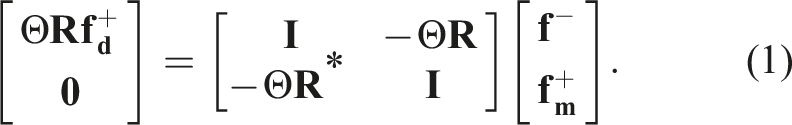
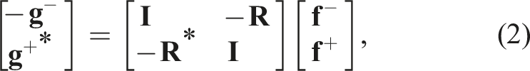
To conclude this section, we briefly summarize how the SRI application works in practice. The overall redatuming process is mostly composed of two phases:

• Pre-processing: TLR compression is applied to each frequency matrix of the seismic dataset. This process is embarrassingly parallel at the frequency level, and it is performed only once upfront with a limited overhead compared to the overall SRI.

• Redatuming: this process entails the repeated solution of the system of equations (1) for a regular grid of subsurface points at a certain depth of interest. The estimated Green’s functions [equation (2)] can be subsequently used to image the portion of the subsurface below the chosen target level. In practical applications, the number of subsurface points can be in the range of one to 10,000.

5. Powering SRI using TLR-MVM

5.1. TLR data compression format

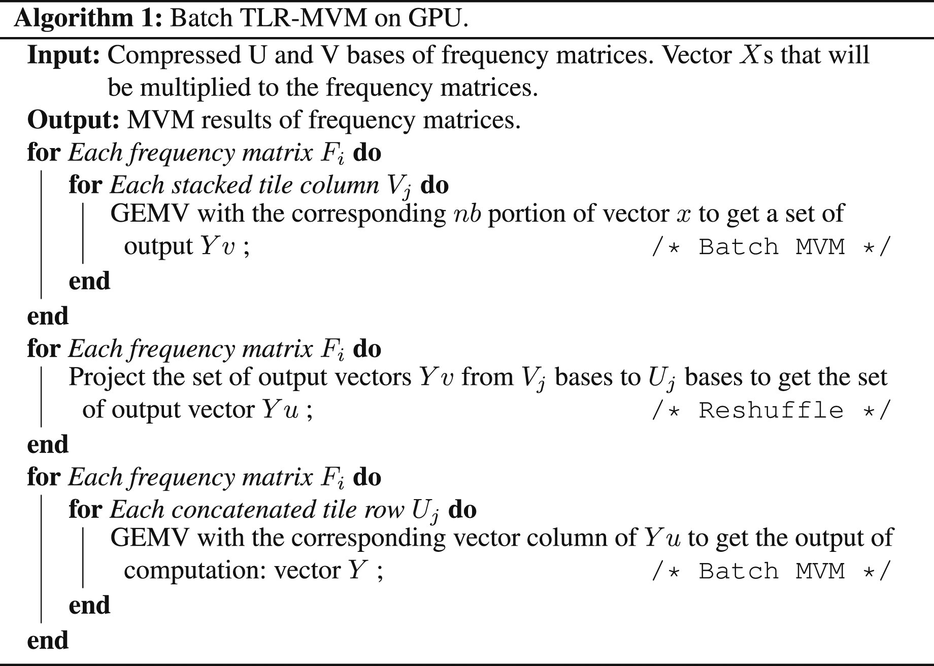
Tile Low-Rank (TLR) matrix approximation (Amestoy et al., 2015); (Akbudak et al., 2017) is a technique that decomposes a dense matrix into tiles (in this article, of equal size) and then performs a singular value decomposition (or some other low-rank decomposition) on each tile. The TLR algebraic compression is done once upfront before starting the SRI workflow. Two orthogonal bases U and V are generated per tile with a rank k that corresponds to the k most significant singular values and their associated singular vectors. The ranks may be different for each tile, which may create load imbalance situations within a batch of TLR-MVMs. The bases are stacked in two groups of left or right bases, respectively, to enhance contiguous memory access in each batched phase to follow. The procedure is then split into three successive phases to perform TLR-MVM for each frequency matrix: (1) the input vector $\tilde{x}$ is multiplied by the U bases via batch MVM with variable sizes due to different ranks k, (2) the output matrix from the previous phase is projected into the V bases via memory shuffle operations, and (3) the V bases are applied to the output from the previous phase using a batch of MVM with variable sizes, again, due to different ranks k. These three phases are described in detail in Ltaief et al. (2021) (Section 4). The algorithm for batch TLR-MVM is schematically described in Figure 1. The overall compression rate turns out to be sensitive to the source-receiver ordering, as explained in the next subsection.

Figure 1.

Memory layout for Phase 1 and Phase 3 of the standard and transpose TLR-MVM. “Nb” is the block size of the tiles and “LD” is the leading dimension of the matrix.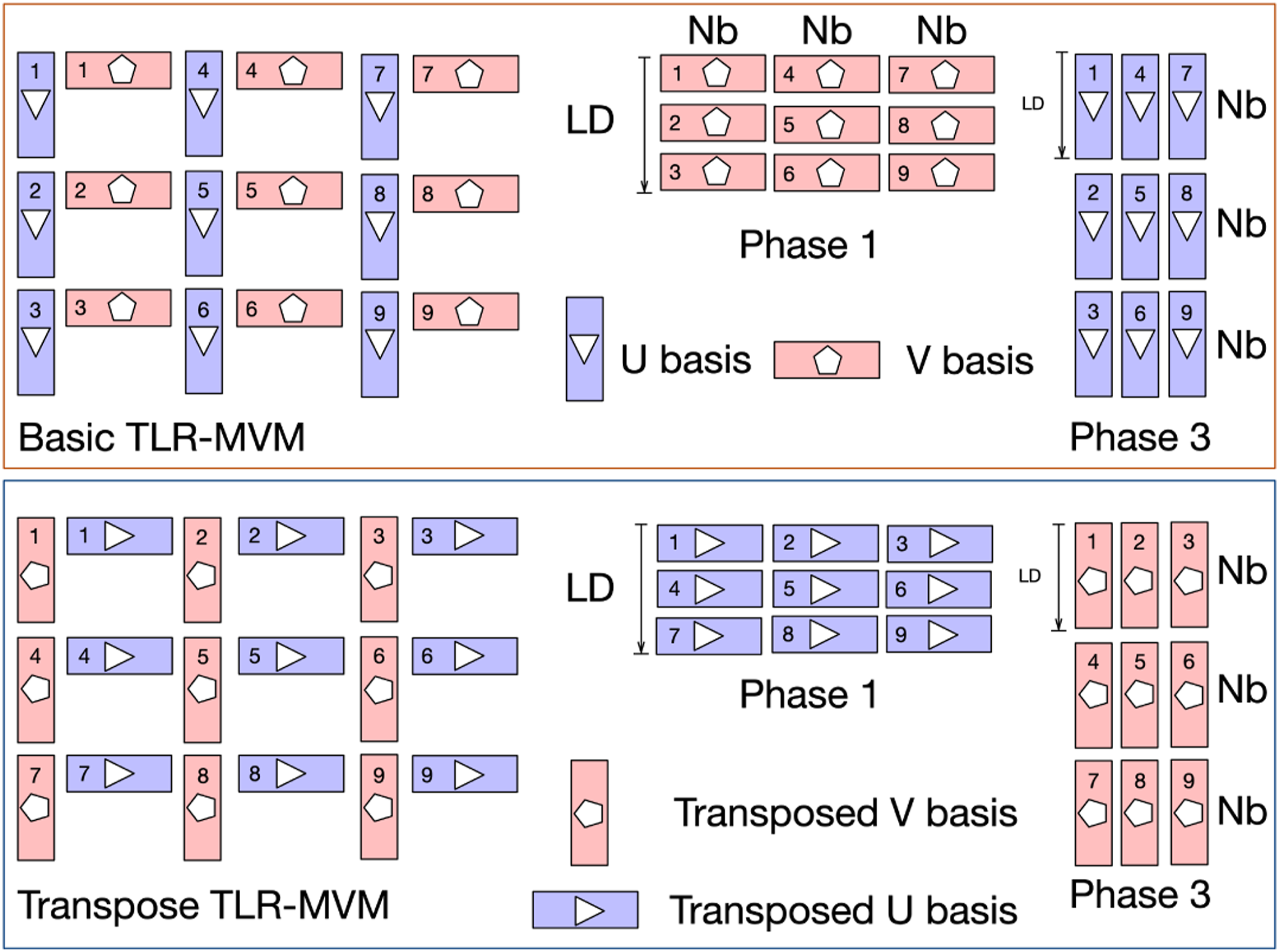

Algorithm 1 describes the batch TLR-MVM approach. Note that there are two nested levels of batching in the algorithm. For each frequency matrix, we perform a matrix-vector multiplication. This represents the first level of batching, which is referred to as batch TLR-MVM. In the first and third phases of TLR-MVM, we replace then the dense MVM kernel and rely on a batch MVM kernel with a variable problem size. This constitutes the second level of batching, known as batch MVM. We will further explain how we implement mixed-precision kernels and utilize the CUDA stream and CUDA graph to accelerate computations in the implementation section.

5.2. Impact of matrix reordering

A seismic reflection response, used here as the kernel of the MDC operator, can be conceptually visualized as a three-dimensional tensor of size N_f × N_s × N_r, where N_f frequency matrices are arranged along the slowest axis, each of them composed of N_s sources (i.e., rows) and N_r receivers (i.e., columns). When performing MDC with such dense frequency matrices, the arrangement of sources (along the rows of each matrix) and receivers (along with the columns of each matrix) is in principle arbitrary as long as it is consistent with that of the input $\tilde{x}$ . The arrangement is, however, important within the context of TLR compression as it may lead to better or worse block compressibility. A variety of reordering strategies that aim at reducing the overall distance between sources (and receivers) within the same tile have been investigated. We display a single frequency matrix (f = 33 Hz) in Figure 2(a) and 2(b), obtained with the original and distance-aware matrix reordering methods shown in Figure 2(c) and 2(d), respectively. We consider this matrix as representative of general trend in the dataset since its total rank summation falls in the interval between the median and third quartile of the whole stack of frequency matrices. Based on Hilbert space-filling curves, the distance-aware reordering permits to the cluster of the highest interactions between nearby sources-receivers mostly around the matrix diagonal and avoids a diffusive pattern, as seen for the naive ordering. Hilbert reordering provides the best compression rate by better leveraging the data sparsity of the frequency matrices. Space-filling Morton (or “Z”) curves have also been considered and are not as effective.

Figure 2.

Single frequency matrix (f = 33 Hz) with default (left) and Hilbert space-filling (right) matrix reordering techniques.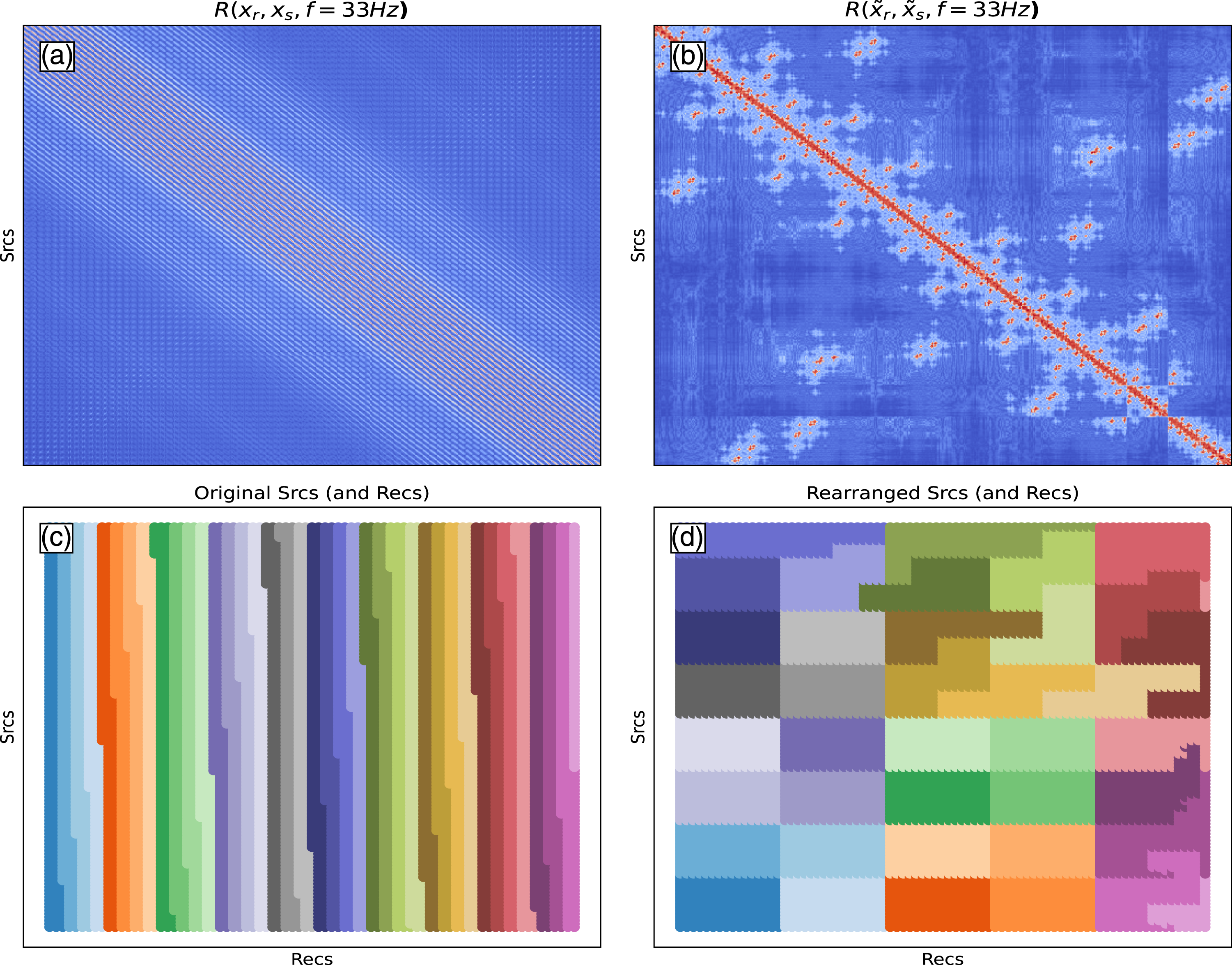

5.3. Impact on SRI computational stages

Whilst in Hong et al. (2021), we focused only on the implementation of the forward batch MVM operation; here, we cover the entire SRI workflow where an iterative solver is used to solve the Marchenko equations. This requires the application of four batch MVM operations as explained in Section 4. We can proceed with the standard TLR-MVM for Rx. For the conjugate TLR-MVM R*x, we can simply apply R to x* and then conjugate the output. Indeed, the conjugate of the product of two numbers is the product of the conjugates and the conjugate of the sum of two numbers is the sum of their conjugates; therefore, element-by-element, the conjugate of ${(R (x^{*}))}^{*}$ is R*x. Using similar reasoning, the conjugate transpose of R^Hy is ${((R^{T}) y^{*})}^{*}$ . In other words, we do not need to explicitly form the conjugate transpose R^H, rather we can simply apply the transpose R^T, which also covers the last operation. In summary, we need to store only R and access it in two different ways, that is, standard and transpose, as illustrated in Figure 1 with a 3x3 tile frequency matrix. The U and V bases can be safely swapped but accessed with a different data layout (from row-major to column-major). By conjugating only the vector and not the compressed matrix generated from the dense R, we do not require any data storage beyond what is required for the original TLR-MVM.

6. Mixed-precision TLR-MVM computations

While TLR-MVM significantly reduces the memory footprint and the overall algorithmic complexity of the MDC operator, it does not improve its arithmetic intensity (determined by the flops/bytes ratio). In fact, its mathematical efficiency reduces its performance efficiency while improving its execution time. Thus, we add the support for mixed-precision computations in TLR-MVM in order to increase the arithmetic intensity by performing the same number of flops but on less data transferred from/to registers. While vendors support lower precision in hardware and/or software, they may not provide all matrix kernels. In particular, given the single complex precision arithmetic required by SRI, the standard batch MVM kernel within TLR-MVM is not supported by any vendor for such data types. Therefore, we decouple the real and imaginary parts of each element of the U/V bases and create our own data type for the half-complex precision composed of two FP16 elements. Moreover, our TLR-MVM implementation is translated from batch MVM into batch tall and skinny matrix-matrix multiplications. While this can be helpful on some architectures, it may still be inefficient on massively parallel devices due to low hardware occupancy. This may require the development of new kernels optimized for memory accesses. Moreover, our approach does not employ casting or scaling/unscaling mechanisms only, as in Fabien-Ouellet (2020), nor computing/storing in higher/lower precision only, as in Flegar et al. (2021). Our approach combines casting and/or scaling/unscaling mechanisms with the high-precision accumulation of the MVM transient results. We actually adopt a similar approach to those of vendor numerical libraries that support, for instance, MP matrix-matrix multiplication kernels (mostly for AI workloads) using operands in FP16 while the operation is done in FP32. All in all, we provide two MP implementations for the TLR-MVM: the first one mixes FP16/FP32, while the second one manipulates INT8/INT32/FP16/FP32, as explained in the next section.

7. Implementation details

In this section, we first recall the original implementation of TLR-MVM (Hong et al., 2021) and provide new details necessary to extend its portability to a wider number of vendor architectures. We then discuss mixed precisions for TLR-MVM and introduce new kernels to support this effort.

7.1. Extending TLR-MVM portability to other systems

In Hong et al. (2021), we implement TLR-MVM in C++ on NEC SX-Aurora TSUBASA vector engine using a standard MPI + OpenMP programming model. A load balancing technique is further introduced to reduce idle times encountered when simultaneously processing all seismic frequency matrices in single complex precision arithmetics. Since the single complex datatype for MVM (i.e., CGEMV) is widely supported by vendor numerical libraries, we propose to further extend TLR-MVM to a wider family of systems, including x86, ARM, and GPU. For x86 and ARM, MPI + OpenMP is also natively supported and portability is attained with modest effort. However, in order to attain maximum performance, the MPI processes and their corresponding OpenMP threads must be mapped carefully into the underlying core/socket packaging. For the GPU implementation (NVIDIA studied herein), MPI remains as the bridge to communicate across GPUs, while the CUDA software ecosystem is used inside the GPU. In particular, we rely on streams to launch the batch MVMs with variable sizes and monitor the data dependencies inside the TLR-MVM computation. These streams are then captured by the CUDA Graph framework for asynchronous execution while reducing the kernel launch overheads observed when operating on small data structures. Figure 3 shows the DAG of TLR-MVM when processing a single frequency matrix with 20 streams. Phases 1 and 3 are embarrassingly parallel and can benefit the most from streams. Since SRI involves many frequency matrices, we merge each phase of TLR-MVM across all frequency matrices to further expose parallelism, reduce CUDA Graph overheads, and increase hardware occupancy. This is also explained in Algorithm 1. Inspired by the merge phase strategy in Hong et al. (2021), we build a single DAG to launch massive operations on all frequency matrices at the same time. We execute Phase 1 of all frequency matrices in a round-robin fashion and synchronize for Phase 2. We then execute Phase 3 for all frequency matrices again in a round-robin fashion until all MVM tasks (i.e., CGEMV) are completed.

Figure 3.

CUDA graph of a single TLR-MVM with 20 streams.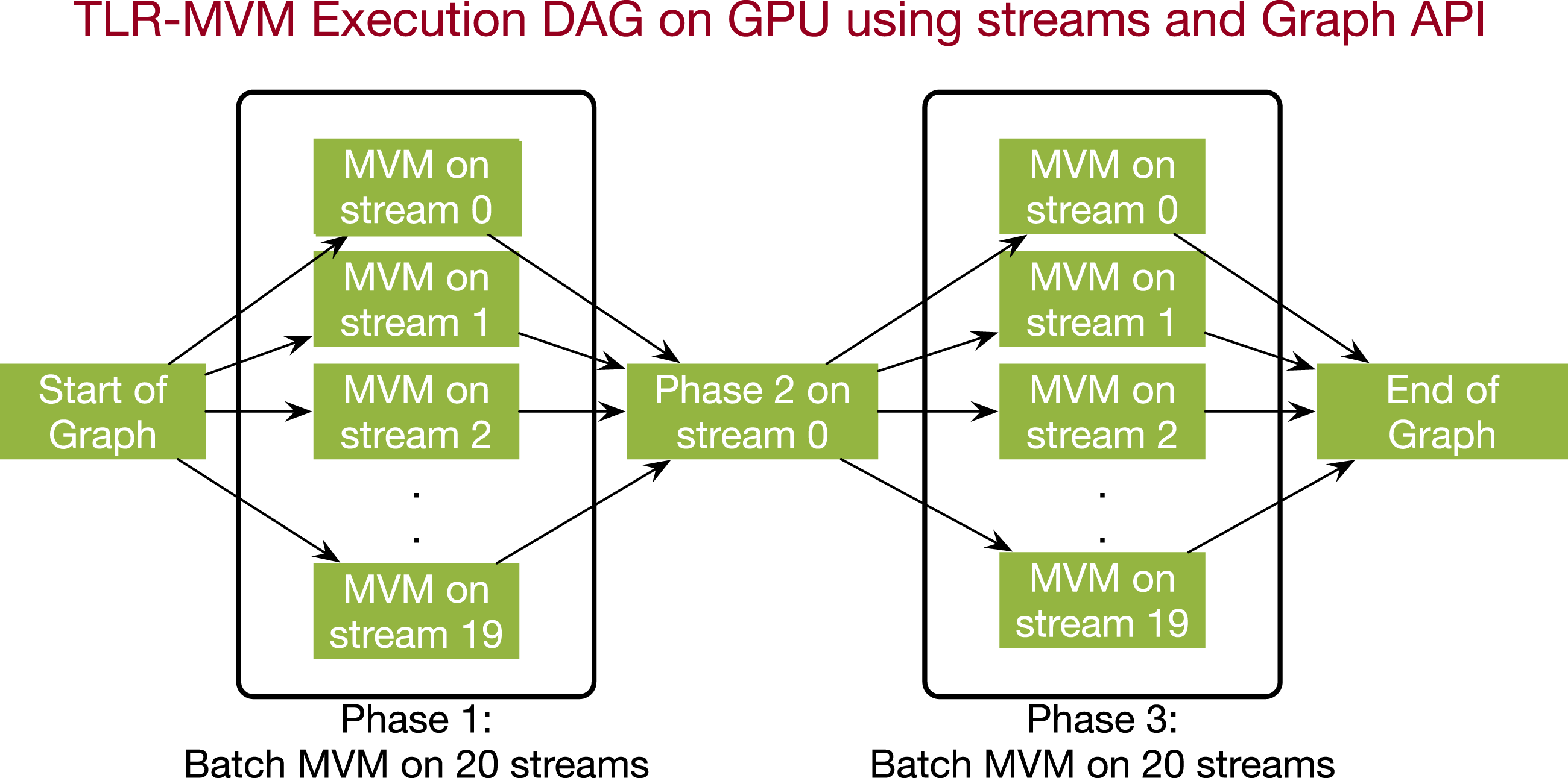

7.2. Mixed-precision TLR-MVM

We here introduce the implementation of two mixed-precision (MP) kernels for our TLR-MVM code: FP16/FP32 and INT8/INT32/FP16/FP32.

7.2.1. Hardware/software limitations for mixed precisions

Unfortunately, not all vendors provide hardware and/or software support for MP involving half-complex arithmetic. We have therefore three choices depending on the level of support. If FP16/INT8 datatypes are not supported, we cannot deploy our kernels on the system. If these two data types are supported, we need at least to have access to numerical libraries with MVM BLAS functionalities that provide FP16/INT8 interfaces. In our experience, the GEMM BLAS function is usually the one enriched with support for such data types. However, replacing our memory-bound MVM kernel with the GEMM kernel operating on a single vector may represent a suboptimal choice. In fact, whilst it may provide portability, it may affect performance. The third option is to design a new kernel that not only fully supports FP16/INT8 datatypes but also performs the MVM operation with memory-aware optimizations to reduce latency overheads. In this article, we introduce new CUDA kernels for the latter, as explained in the next section.

7.2.2. MP TLR-MVM using FP16/FP32

In this section, we discuss the design of our FP16/FP32 MVM kernel, which is the main building block of MP TLR-MVM using FP16/FP32. To begin with, a new struct that contains two half numbers is defined as the FP16 complex data type. We carry on the implementation using this new data type. The input U/V bases of the matrix R are assumed to be in FP16.

7.2.2.1. Vectorized global memory access

We set block size to 128 and each warp (32 CUDA cores) handles every four rows/columns of the MVM kernel when manipulating the input U/V bases. We choose a block size of 128 threads for two reasons. The first is that block sizes should be a multiple of 32 since each warp is in charge of many rows and we want to maintain fine granularity. Each warp processes 4 rows (MP FP16 TLR-MVM)/8 rows (MP IN8 TLR-MVM) per iteration. This means that each block processes 16/32 rows at a time. A coarser block size of 256/512 may also be acceptable although it may eventually reduce the hardware occupancy. The second is to get coalesced memory access for both input U/V bases and input vector. We use 128-bit loads and stores as much as possible. Since each element of the U/V bases is two half numbers (32 bits), we need four half-complex numbers stored contiguously to trigger 128-bit loads and stores. Since U/V bases are column-major, this means one thread needs to access four rows/columns at a time. For instance, for Phase 1, each thread loads four elements from the vector, once at a time, which means the threads also need to access the four columns of matrix U bases. To ensure the vectorized access, we cast the input pointer to float4 and reinterpret_cast is used. Figure 4 shows the design of how we assign the entries of U/V bases to different CUDA cores.

Figure 4.

Vectorized access and CUDA block layout for FP16 complex MVM kernel.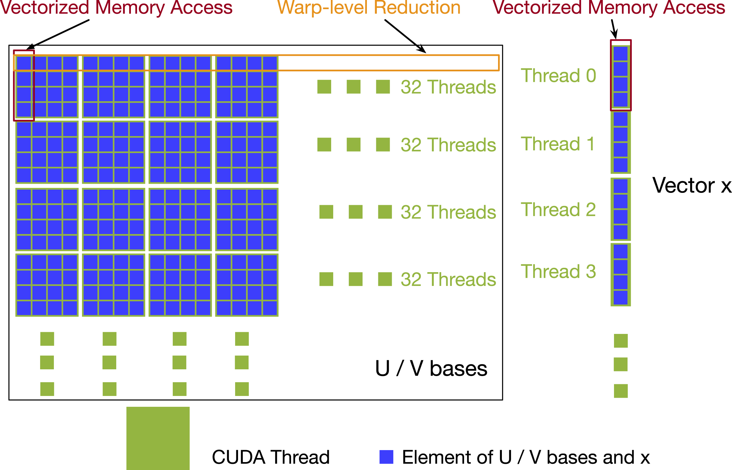

7.2.2.2. Warp-level reduction

We use warp-level reduction for row reduction. After looping through the rows, the CUDA cores inside the same warp use __shfl_down._sync to exchange the partial reduction results. After the operation, the first thread inside the warp will have final results. We again cast the four cuComplex numbers as float4 to maximize occupancy. Since BF16 is also supported on CUDA, we also provide BF16/FP32 MP TLR-MVM following the same optimizations described in this section.

7.2.3. MP TLR-MVM using INT8/INT32/FP16/FP32

We extend the vectorization and reduction optimizations for MP-TLR-MVM to support even lower precisions. The input U/V bases of R are assumed now to be in INT8 precision. However, as the original seismic data may not fall in the range of INT8, for example, [-128,127], we downscale the real/imaginary part of each U/V base separately into INT8 precision using their maximum absolute value. In this way, we can preserve the information in the matrix as well as execute the MVMs in INT8 for TLR-MVM with limited precision loss. We now define a struct that contains two int8_t as INT8 Complex data type. In the same manner, we operate on 16 INT8 datatypes together to use 128-bit loads and store as much as possible. We access the V bases of R in the same manner, following Figure 4. We can launch Phase 2 with memory shuffling. We scale only at the end of Phase 2 by taking all FP16 entries and converting them to INT8. We can then launch Phase 3 where we read the U bases of R in INT8 and multiply them against the INT8 results coming from Phase 2. In the end, we remark that our code for supporting INT8 entries for U/V bases is required to operate on four different precisions. Figure 5 shows workflow of FP32 TLR-MVM and MP INT8 TLR-MVM.

Figure 5.

Workflows of FP32 and MP INT8 TLR-MVMs.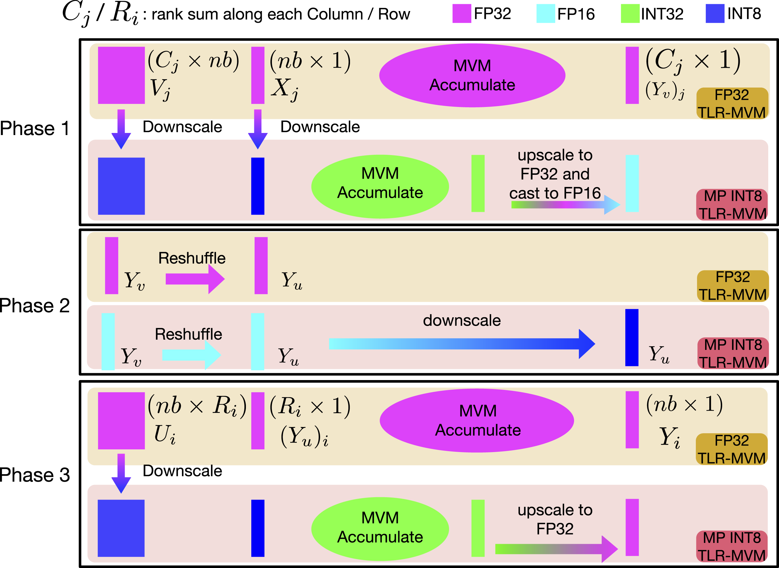

8. Numerical accuracy

In this section, the proposed TLR-MVM implementation is applied to the same synthetic geological model used in Ravasi and Vasconcelos (2021); Hong et al. (2021). The choice of this dataset is motivated by the fact that extensive numerical analysis has been previously performed with respect to the capabilities of SRI in 3D scenarios. Our focus here is orthogonal, in that we want to assess the potential impact of TLR and MP on the quality of the solution. The model extends over an area of 1.8 km × 1.2 km x 1 km and comprises several horizontally stacked layers and a syncline-like structure in the overburden, which leads to the generation of complex scattering events in the recorded seismic dataset. The seismic dataset is created using a finite-difference acoustic modeling code from a regular grid of 9801 co-located sources and receivers. The collection of shot gathers is stored in FP32 precision for a total size of 230 GigaBytes (GB). The dataset is further converted to the frequency domain as required by MDC operators, and only the first 150 frequency components (0 < f < 50 Hz) are retained for further computations (note that this is not a hard constraint of our application and a larger bandwidth could be selected). The kernel R becomes therefore a complex-valued, three-dimensional tensor of size 150 × 9801 × 9801, whose real and imaginary components are stored in FP32 format for a total size of 115 GB. Finally, all of the numerical results presented below will be shown for a single focusing point in the subsurface at location x_F = (580, 620, 650)m. We refer the reader to Ravasi and Vasconcelos (2021) for more details on the dataset itself.

In the following, we wish to study the impact of our implementation of the MDC operator on the overall accuracy of the SRI application. The wavefields obtained by inverting the system of equations (1) are compared for different choices of floating-point precisions used to store the bases of the TLR compressed R kernel. The Signal-to-Noise Ratio (SNR) measurement, SNR = 20* log₁₀‖x_true‖₂/‖x_true − x_approx‖₂, is used quantify the error resulting from the different algebraic and numerical approximations introduced in this article. For all of the examples, x_true corresponds to the true wavefield computed numerically in the true model using the same finite-difference acoustic modeling code used to create R kernel, whilst x_est refers to the estimated wavefields using any of the approximations discussed in this article. Note that the true solution is obviously not available in real-life applications when we cannot access the exact subsurface models.

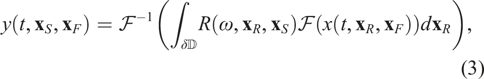
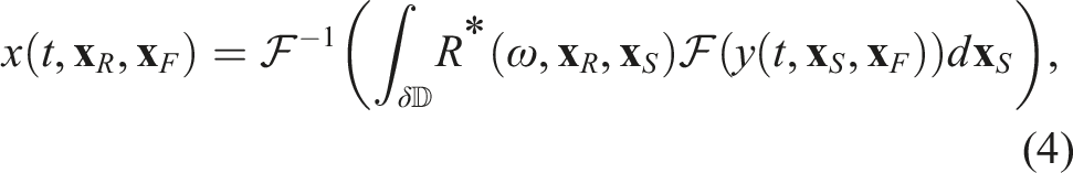
To begin with, let us briefly discuss how each of the frequency matrices used to perform the forward and adjoint operations in equations (3) and (4) are formed and how they relate to the physical seismic acquisition geometry. A schematic representation of a seismic acquisition geometry is displayed in panel (a) of Figure 6 alongside a single frequency matrix of the kernel R (panel (b) of Figure 6). As commonly done in geophysical processing, the data recorded from sources to receivers along lines L_i is organized such that sources and receivers correspond to rows and columns in the matrix, respectively. The overall matrix can be therefore be interpreted as a stack of smaller matrices where each of these submatrices contains sources from line L_i and receivers from line L_j. Note that the choice of the tile size for the TLR compression algorithm can, but does not need to, follow the structure of these “geographical” blocks. Given this arrangement of the kernel matrix, a possible approach is to divide the entire matrix into two bands: tiles inside the inner band are compressed as usual and stored in FP32 precision, whilst tiles in the two outer bands are discarded (i.e., set to zero). By doing so, we are implicitly assuming that contributions to the integrals in the equations (3) and (4) from receiver lines away from the source of interest have less impact on the overall modeling (or inversion) outputs than those from nearby receivers. Although this may seem like a reasonable argument to make, panels (c) and (d) in Figure 6 show that this is not the case: both the far away and nearby receivers are in fact required in order to fully construct the seismic events when applying the forward modeling operator. More specifically, events in the reflection data [thick rays in panels (c) and (d)] that experience a bounce with a subsurface reflector below the focus point generally require far away receivers (e.g., $x_{R}^{1}$ ) past the focusing point x_F to be captured, whilst those that have a shallow bounce require nearby receivers (e.g., $x_{R}^{2}$ ). Based on these physical arguments, we will see that only in the case we are interested to keep high accuracy in the reconstruction of events at a small offset (i.e., a small distance between the horizontal location of the focusing point and a given receiver) whilst accepting a large degree of error for those at far offset, does zeroing out the off-diagonal tiles represent an acceptable trade-off between accuracy and computational cost. In general, as we are interested in recovering both near and far offset events, the zero-out approach is not appropriate and should be avoided. We have however decided to include it here as a matter of comparison to smarter approaches that reduce the memory footprint of the MDC operator by carefully reordering the rows and columns of the seismic frequency matrices and lowering their overall precision.

Figure 6.

(a) Acquisition geometry, where sources/receivers are distributed along N black lines L₁, L₂, …, L_N. Red stars and blue triangles refer to sources/receivers used in the panels below. A single black dot indicates the focusing point. (b) Single frequency matrix of the kernel R with blocks corresponding to some of the acquisition lines. (c)–(d) Subsurface cross-sections along the thin dashed line in panel (a) with raypaths corresponding to events to be constructed by the forward modeling operator in equation (3). Such schematic diagrams show that some of the physical events are created using nearby pairs of sources and receivers [panel (d)], whilst others require pairs of far away sources/receivers [panel (c)].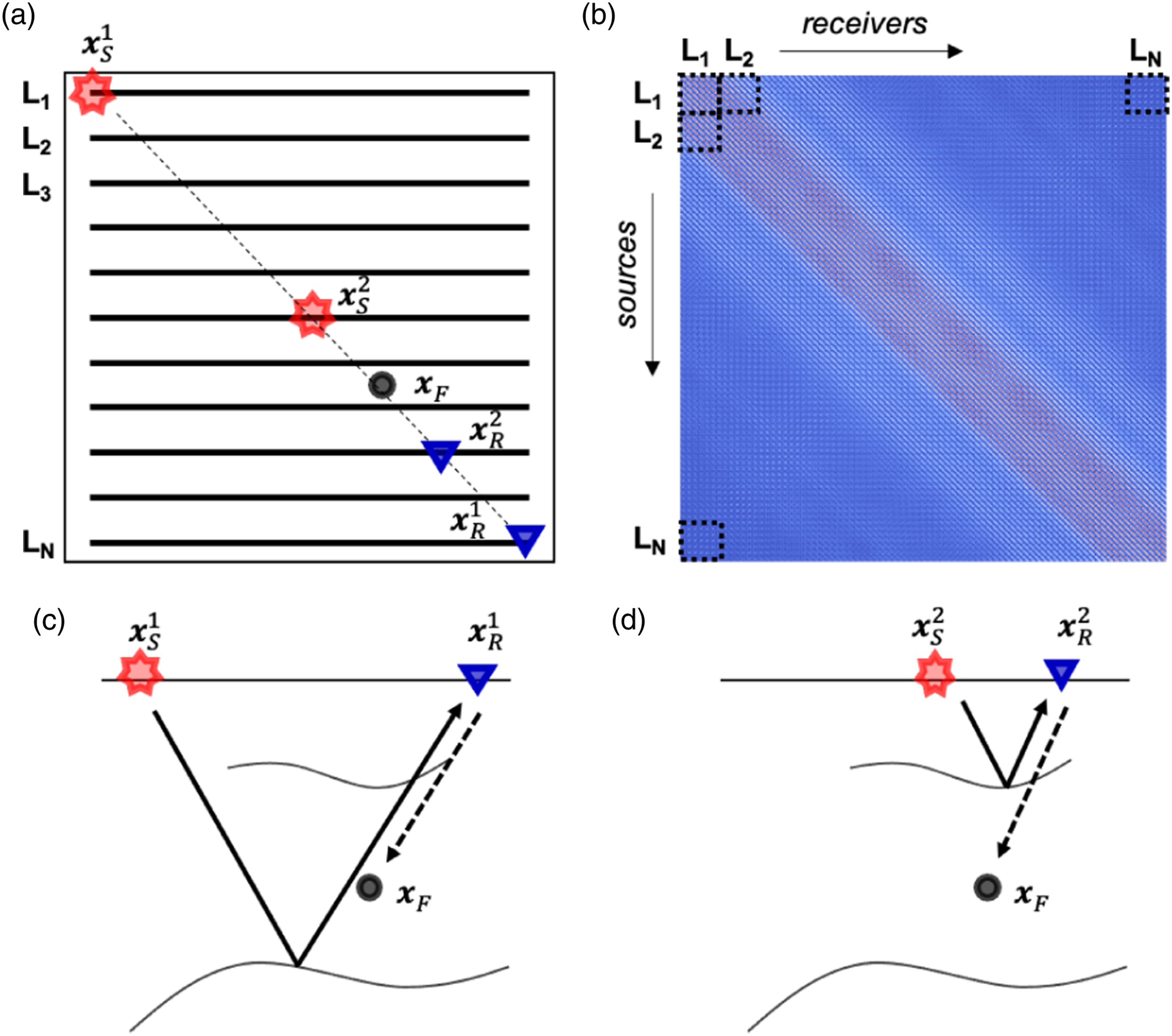

Figure 7 presents a comparison of a variety of inversion results (i.e., the final total Green’s function g) along eight different receiver lines, as shown in the insert. In all cases, TLR compression is performed using the following parameters: tile-size nb = 256 and accuracy ϵ = 0.001—for a more in-depth analysis on the choice of the parameters nb and ϵ and their impact on the quality of the solution we refer the reader to Hong et al. (2021).

Figure 7.

Wavefields obtained by applying the entire inversion [equations (1) and (2)] using TLR compressed R kernel and different precisions. (a) FP32, (b) FP16, (c) INT8 (d), (e), and (f) corresponding errors with normal ordering. (g), (h), and (i) corresponding errors with Hilbert ordering. (l) SNR for all of the precisions discussed in the main text.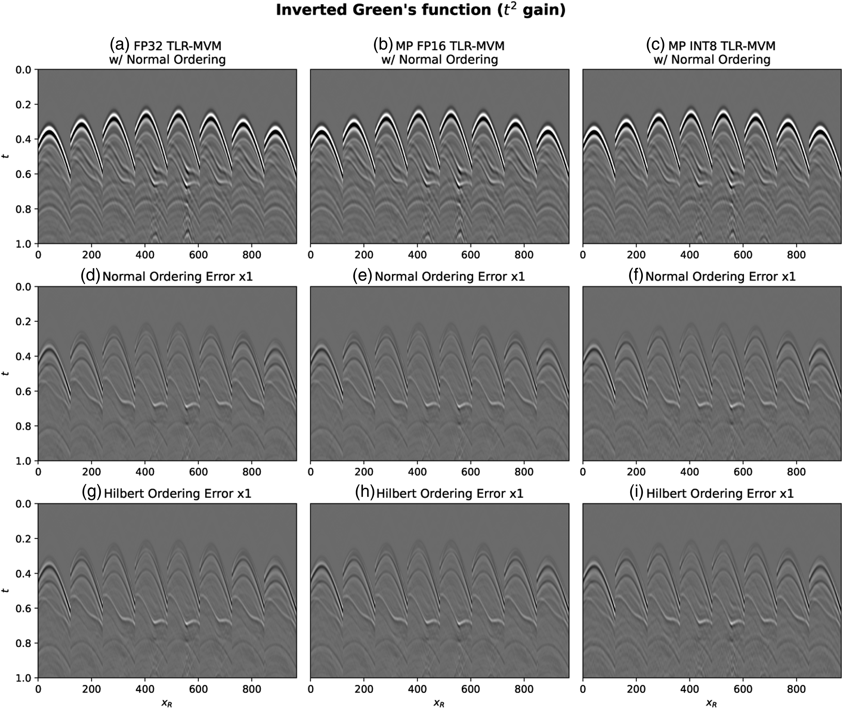

Panel (a) presents the wavefield obtained using TLR compression on the normal ordering kernel and FP32 precision. This result is equivalent to that previously presented in Hong et al. (2021), which has been shown to be nearly identical to that obtained by a classical implementation of the MDC operator that uses a dense, FP32 kernel R.

Panel (d) displays the error of the estimated wavefield with respect to the true solution. Two key observations can be made at this point: i) the solution of equation (1) inevitably introduces an error due to the fact that we are discretizing and truncating a spatial integral [equations (3) and (4)]—we will call this theoretical error as it arises independently of the algorithmic choices made in the implementation of the MDC operator; ii) as shown in panel (l), the SNR of the solution obtained using TLR compression is nearly identical to that obtained by using the dense kernel as previously discussed in Hong et al. (2021). This gives us confidence that TLR compression is suitable for the SRI application.

Finally, panel (g) displays the error associated with the scenario where the frequency matrices of the kernel R are re-arranged using Hilbert sorting prior to compression. These results highlight the importance of Hilbert sorting, as it not only lowers the overall size of the dataset to be stored and used for computations as we will discuss later in more detail (see Figure 5), but it does so without compromising the quality of the inversion product.

Next, we start to lower the precision used to represent the real and imaginary parts of all of the U and V bases of the kernel matrices. More precisely, FP16 and INT8 are used to produce the wavefields in panels (b) and (c), respectively. Once again, when looking at the corresponding error panels both with original and Hilbert ordering [namely, panels (e–f) and (h–i)], we can conclude that the entire inversion can be safely carried out using lower precision arithmetic both for storage and computations. This is also confirmed by the computed SNRs shown in panel (l), which are nearly identical for the dense, FP32, and FP16 cases and just slightly smaller for the INT8 case. Figure 8 plots the SNR for all the methods presented in this article. The SNR of BF16 is very close to that of FP16. The difference between corresponding SNR on both Hilbert ordering and normal ordering is less than 0.01.

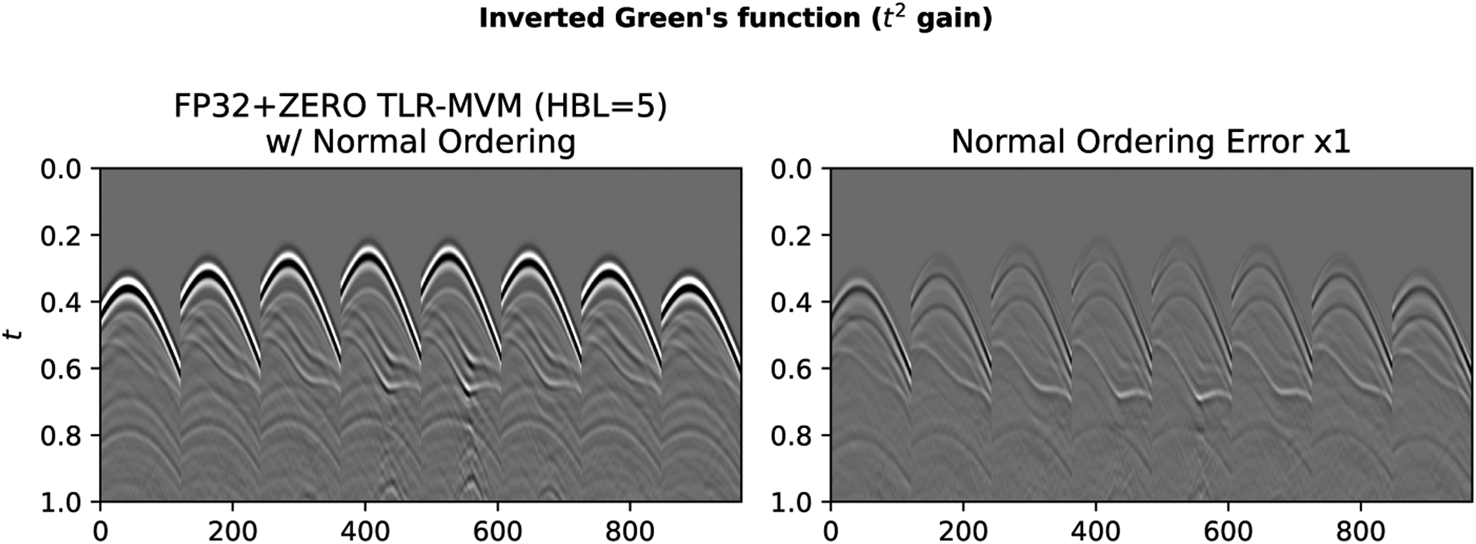
For the sake of comparison and for a sanity check, we also consider the FP32+ZERO with normal ordering strategy where FP32 precision is used for all the tiles in the inner band whilst tiles in the two outer bands are zeroed out. The results are presented in Figure 9. Here, the size of the inner band is defined via the Half Band Length (HBF) parameter. The figure displays the estimated wavefield for HBF = 5 meaning that the inner band is composed of 5 tiles around the main diagonal, whilst the rest of the tiles constitutes the outer band. In FP32+ZERO with normal ordering case, the error clearly increases. More importantly, when looking at the SNR panel, we can conclude that the FP32+ZERO with normal ordering strategy is not appealing in when choosing a HBF = 5 that leads to comparative data size to the INT8 case, the SNR is about 3 dB lower than that of the INT8 case. Even though these off-diagonal tiles may contain low contributions, they simply cannot be ignored. We also present FP32+ZERO with Hilbert ordering strategy in SNR panel for comparison.

Figure 8.

SNR of all the TLR-MVM variants discussed in the main text.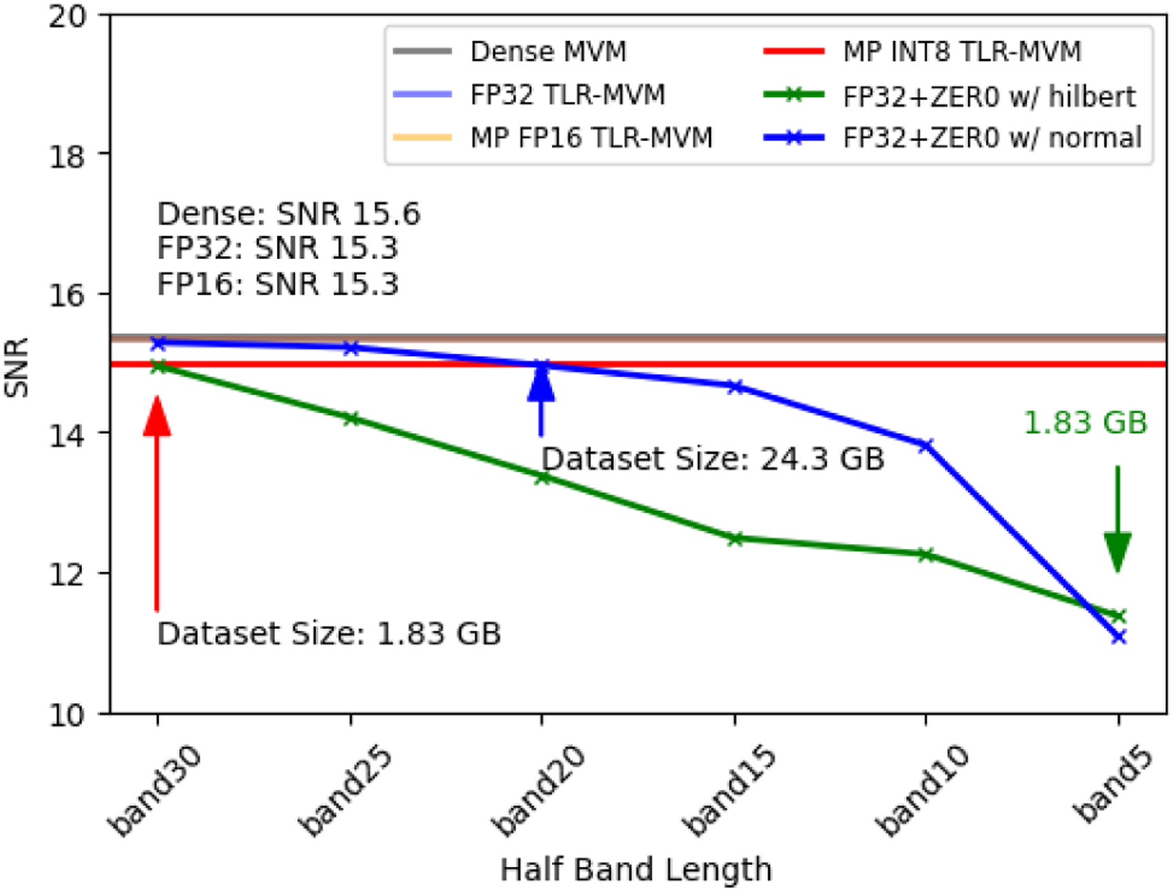

Figure 9.

Wavefields obtained by applying the entire inversion [equations (1) and (2)] using FP32 TLR-MVM in the diagonal blocks and zero in the off-diagonal blocks.

Finally, to further assess the INT8 and FP32+ZERO strategies, a single trace comparison for receivers 1000 and 4000 is shown in Figure 10. An amplitude gain of t² is applied to all traces. Once again, we can observe a good match between the estimate from the INT8 strategy (blue trace) and the original dense-based approach (red line). Similarly, both of them match pretty well the ground truth solution (black lines) apart from small discrepancies. On the other hand, the trace obtained using the FP32+ZERO deviates from the true solution, especially for receiver 1000, which corresponds to the far offset case.

To conclude, we wish to remark that the wavefields shown in Figures 7 and 8 are obtained by solving equation (1), followed by the evaluation of equation (2). Noting that two integral operators must be evaluated in each forward pass of the Marchenko equations (and two in each adjoint pass), the kernel is applied 42 times to obtain the Green’s function when solving the system of equations with 10 iterations of CGLS. This may raise some concern as to whether the solver is sensitive to the accumulation of small approximation errors due to the TLR compressed kernel (especially when compression is used alongside lower precision, e.g., FP16 or INT8). However, our numerical results show the reconstructed Green’s functions with different choices of precision are indistinguishable from the one obtained using FP32 precision (Figure 7(a)).

9. Performance analysis

9.1. Environment settings

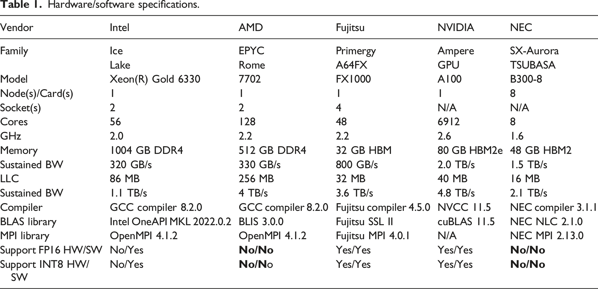
Our numerical experiments are carried out on five architectures, that is, Intel Ice Lake (codenamed ICX), AMD Epyc Rome (Rome), Fujitsu A64FX (A64FX), NEC SX-Aurora TSUBASA (Aurora), and NVIDIA A100 GPU (A100). A detailed hardware and software description is provided in Table 1. We report performance from the median obtained out of 5000 runs. We focus first on the TLR-MVM performance on A100 before extending results to other platforms.

Table 1.

Hardware/software specifications.

Vendor	Intel	AMD	Fujitsu	NVIDIA	NEC
Family	Ice	EPYC	Primergy	Ampere	SX-Aurora
	Lake	Rome	A64FX	GPU	TSUBASA
Model	Xeon(R) Gold 6330	7702	FX1000	A100	B300-8
Node(s)/Card(s)	1	1	1	1	8
Socket(s)	2	2	4	N/A	N/A
Cores	56	128	48	6912	8
GHz	2.0	2.2	2.2	2.6	1.6
Memory	1004 GB DDR4	512 GB DDR4	32 GB HBM	80 GB HBM2e	48 GB HBM2
Sustained BW	320 GB/s	330 GB/s	800 GB/s	2.0 TB/s	1.5 TB/s
LLC	86 MB	256 MB	32 MB	40 MB	16 MB
Sustained BW	1.1 TB/s	4 TB/s	3.6 TB/s	4.8 TB/s	2.1 TB/s
Compiler	GCC compiler 8.2.0	GCC compiler 8.2.0	Fujitsu compiler 4.5.0	NVCC 11.5	NEC compiler 3.1.1
BLAS library	Intel OneAPI MKL 2022.0.2	BLIS 3.0.0	Fujitsu SSL II	cuBLAS 11.5	NEC NLC 2.1.0
MPI library	OpenMPI 4.1.2	OpenMPI 4.1.2	Fujitsu MPI 4.0.1	N/A	NEC MPI 2.13.0
Support FP16 HW/SW	No/Yes	No/No	Yes/Yes	Yes/Yes	No/No
Support INT8 HW/SW	No/Yes	No/No	Yes/Yes	Yes/Yes	No/No

9.2. Performance impact of GPU streams on TLR-MVM

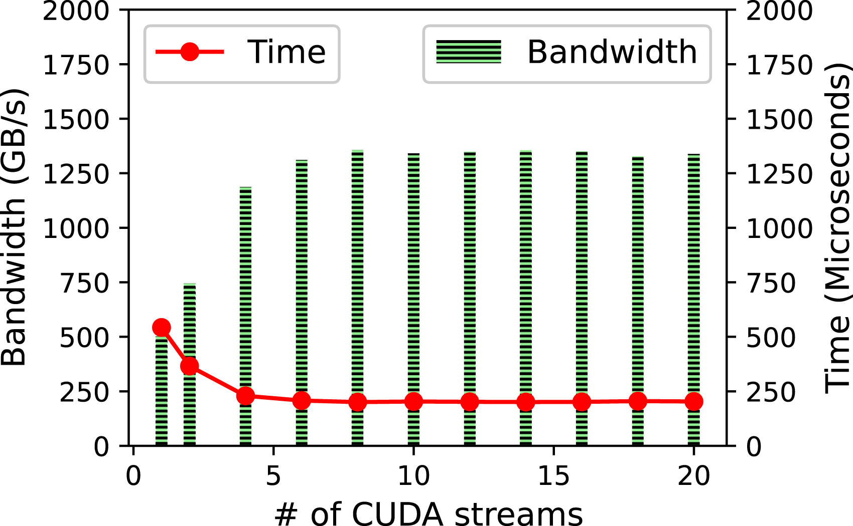
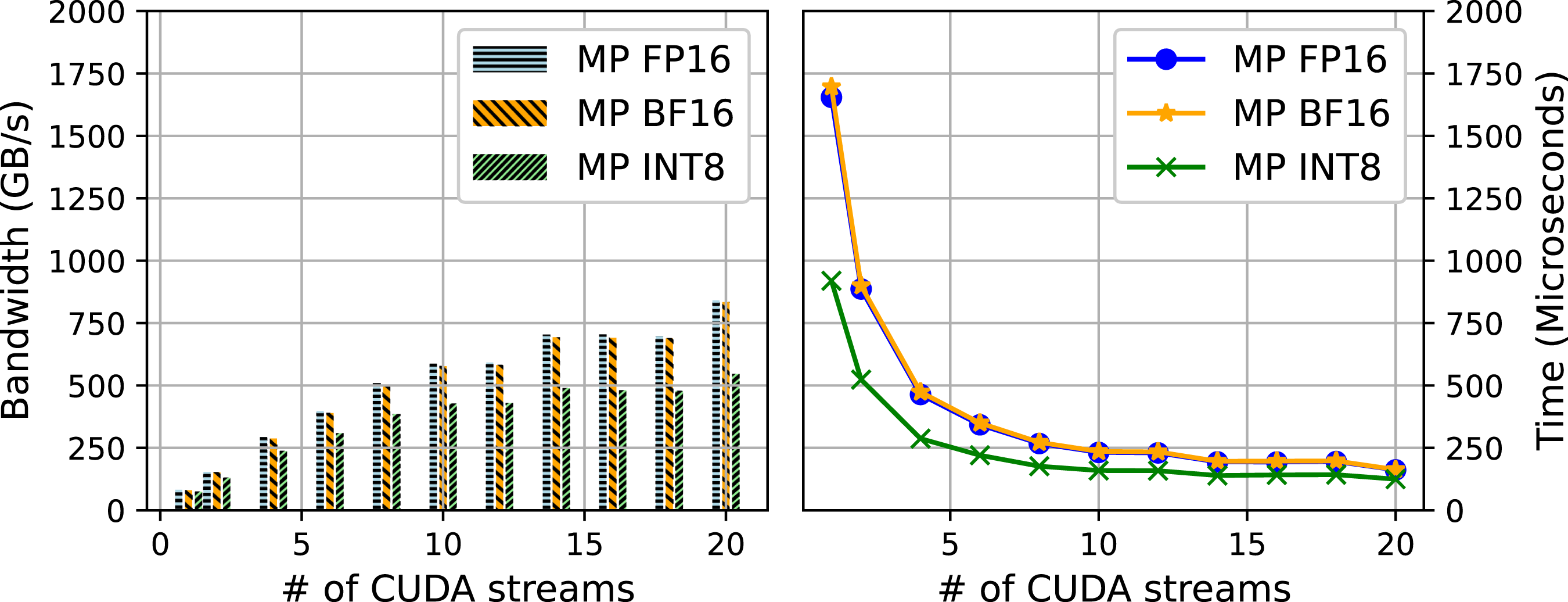
We first study the impact of the number of CUDA streams on the TLR-MVM performance. We use a single frequency matrix f = 33 Hz as a proxy of the overall frequency matrices. Figure 11 displays the bandwidth and time to solution of FP32 TLR-MVM using A100 as function of CUDA streams. The number of streams has a direct impact on the level of concurrency, as described in Figure 3. The bandwidth starts saturating at around eight streams for FP32 TLR-MVM (70% of the sustained bandwidth), reaching up to 2.5X speedup compared to single-stream execution. Figure 12 shows similar performance impact on TLR-MVM when using mixed precisions FP16/FP32 (i.e., MP FP16), BF16/FP32 (i.e., MP BF16), and INT8/INT32/FP16/FP32 (i.e., MP INT8). The bandwidth of MP FP16, MP BF16, and MP INT8 keep improving as we increase the number of streams. This is an indication that there is room to further maximize hardware occupancy, especially when operating on smaller data structures than pure FP32 TLR-MVM. At 20 streams, MP INT8 TLR-MVM eventually runs faster than MP FP16/MP BF16 TLR-MVM, which in turn runs faster than FP32 TLR-MVM, thanks to a higher arithmetic intensity. There is no significant difference between MP FP16/MP BF16 in terms of performance, reaching the same conclusion as for the accuracy assessment in Section 8.

Figure 10.

Trace comparisons of receivers 1000 (left)/4000 (right) for the full wavefield with a t² amplitude gain.

Figure 11.

Performance results of #streams on TLR-MVM using one NVIDIA A100.

Figure 12.

Performance results of #streams on TLR-MVM using one NVIDIA A100.

Figure 13.

Time breakdown of 150 TLR + MP-MVMs on A100.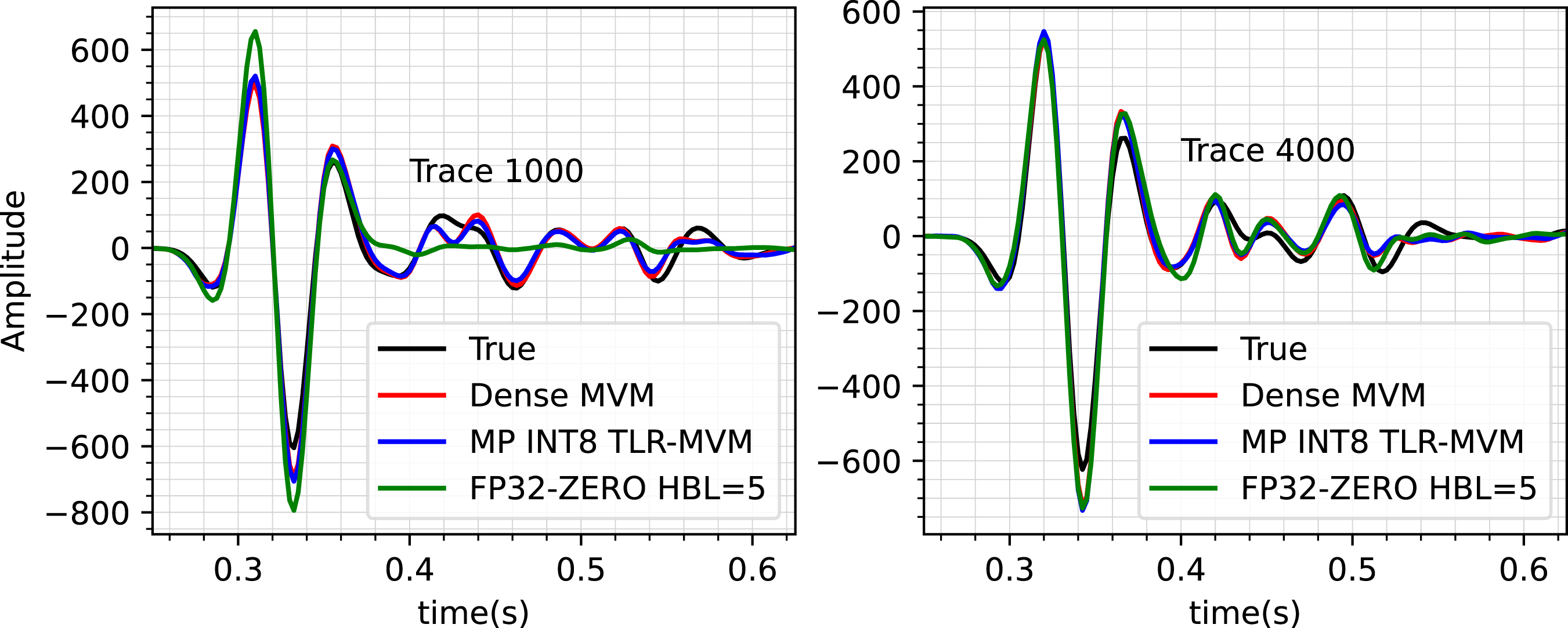

9.3. Impact of matrix reordering and MP on TLR-MVM

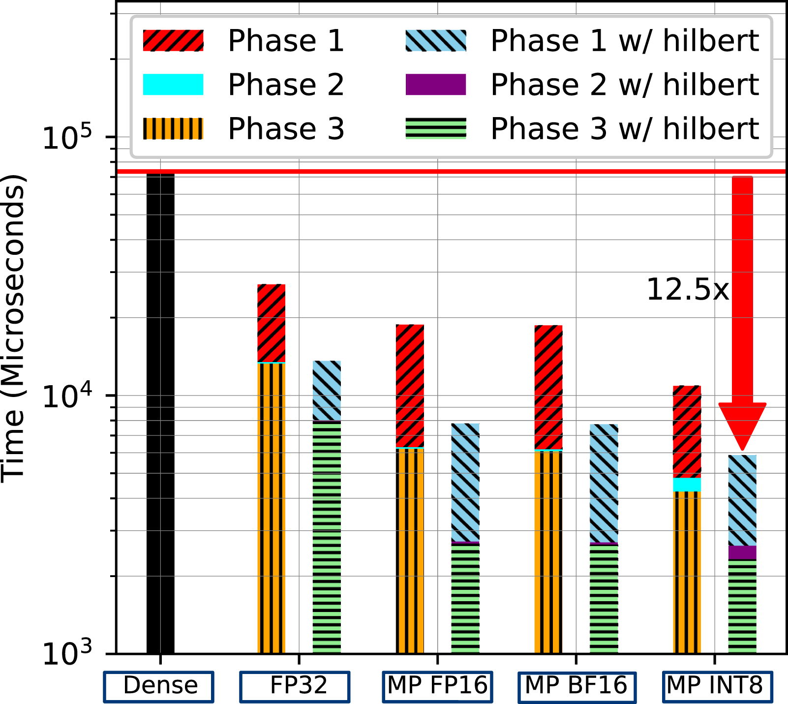
We now assess the performance of matrix reordering with various mixed-precision computations on the TLR-MVM algorithm executed with all the 150 frequency matrices of the seismic dataset. Figure 13 compares them against dense MVM and the reference pure FP32 TLR-MVM implementation using A100. First, it is important to mention that not all of the dense matrices fit in the A100 memory (115 GB $>$ 80 GB), so for the dense MVM, we simply multiply a single MVM time to solution by 150. However, thanks to algebraic compression and matrix reordering, all matrices in FP32 TLR-MVM can fit into the memory of a single A100. Now, looking at the MP variants of TLR-MVM, we see that FP16 or BF16 TLR-MVM perform similarly. Moreover, Phase 3 takes more time than Phase 1 due to the shape of the stacked U (short and wide) and V (tall and skinny) matrices during batch MVMs, respectively. Indeed, the former requires reduction steps while the latter is embarrassingly parallel, during a single MVM. When we activate the INT8 MP variant of TLR-MVM (that in fact requires four precisions, as explained in Section 7.2.3), we get additional performance improvement and reach up to 12.5X speedup compared to dense MVM. Phase 2 takes more time in this MP variant due to the additional scaling operation.

Figure 14 highlights the incremental impact of matrix reordering on the memory footprint of TLR-MVM. TLR-MVM achieves 4X/17X memory footprint reductions against dense MVM with normal and Hilbert matrix reordering, respectively. When MP INT8 variant is enabled, this ultimately translates into a 63X reduction in memory footprint compared its dense counterpart.

Figure 14.

Memory footprint.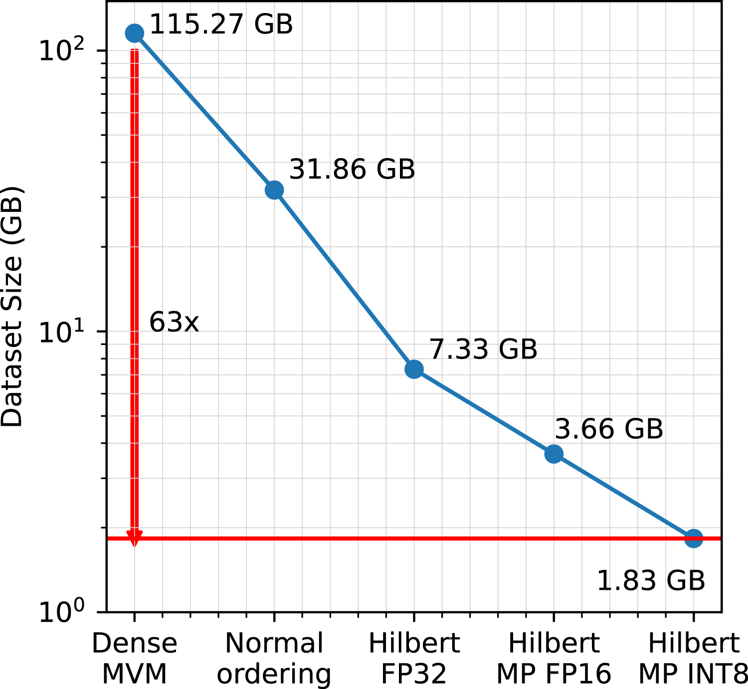

9.4. Performance scalability and roofline of MP TLR-MVM

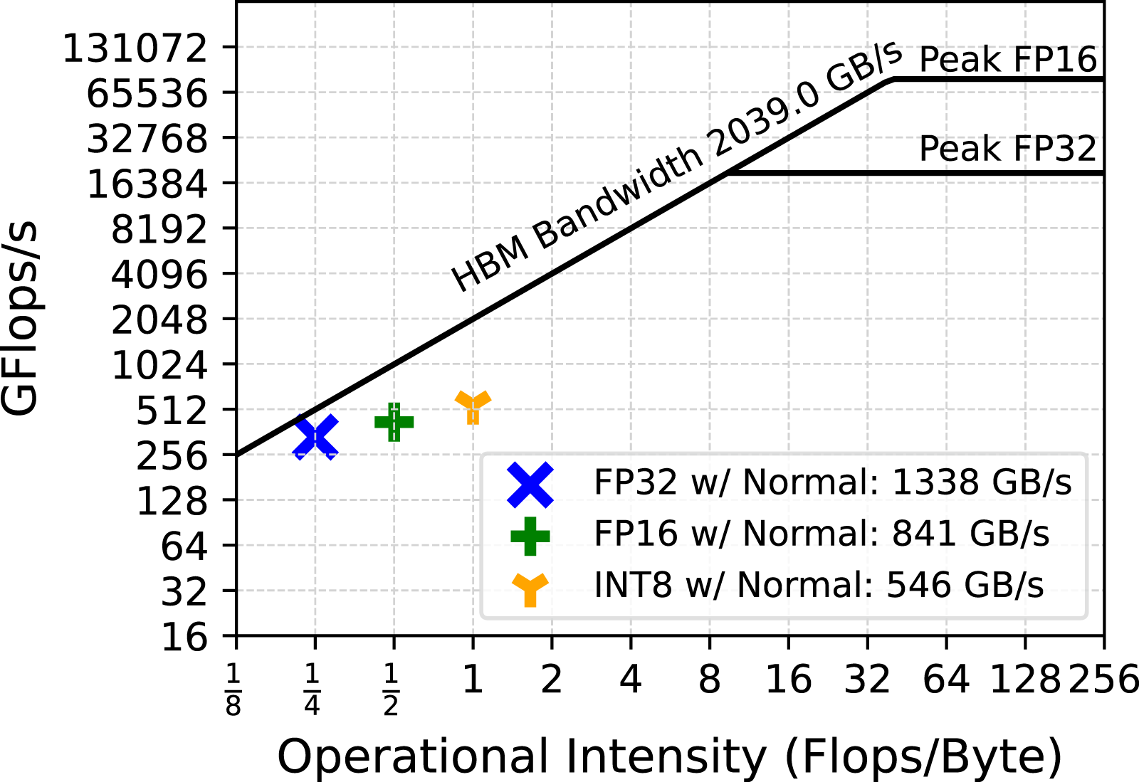
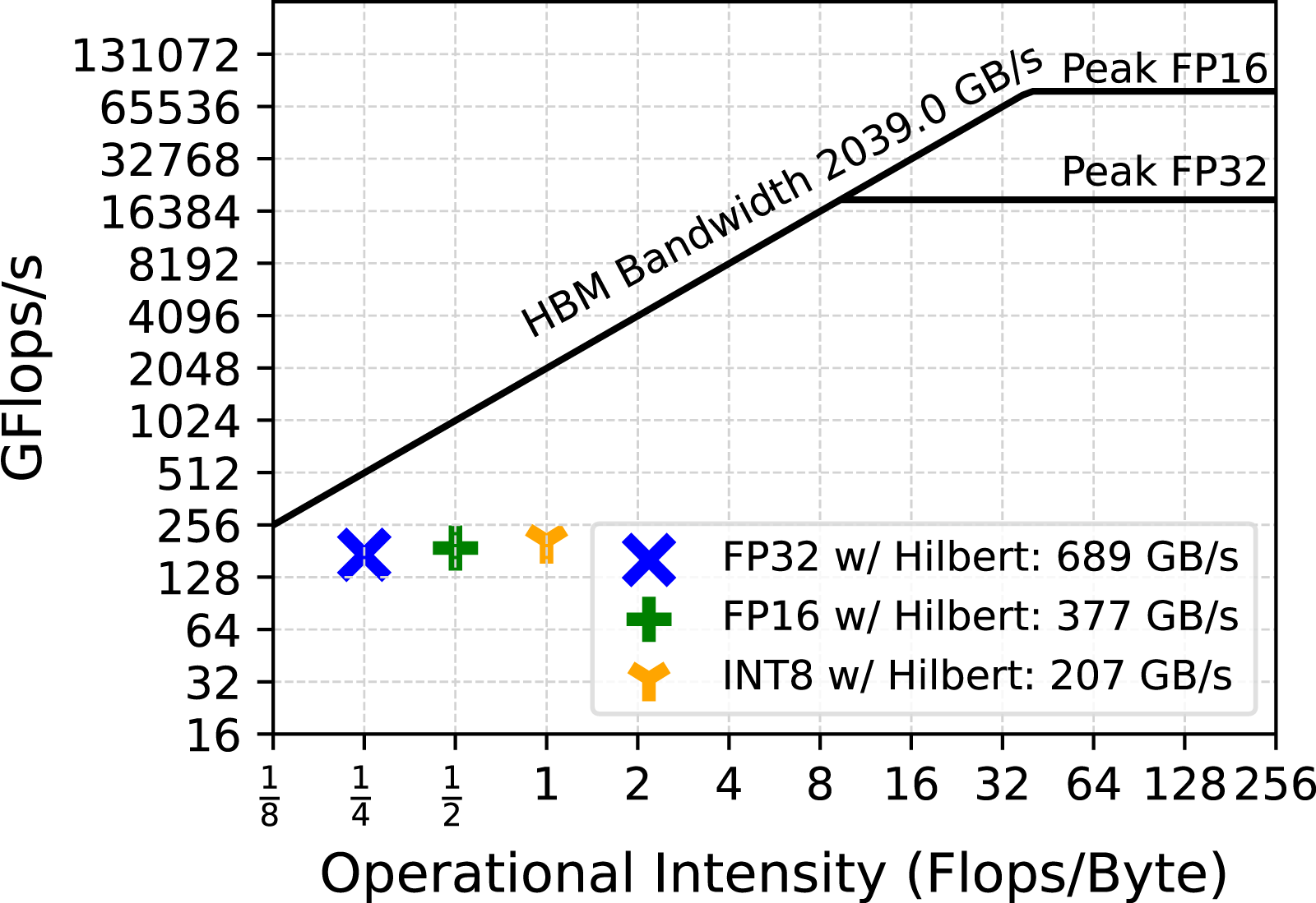
Finally, an analysis of the scalability of the various MP variants of our TLR-MVM algorithm is shown in Figure 15, for processing all frequency matrices and one through eight A100s. Our various implementations deliver linear scalability, given the massive parallelism exposed to the CUDA Graph via streams, as explained in Section 7.1. Moreover, Figure 16 and Figure 17 show the roofline performance model of our MP TLR-MVM kernel with normal/Hilbert matrix reordering, respectively. We see an increase of the arithmetic intensity with MP enabled, since we stream less data volume from main memory. We can further saturate and reach higher sustained bandwidth with larger datasets, while ultimately remaining faster with Hilbert.

Figure 15.

Linear scalability.

Figure 16.

Roofline w/Normal ordering.

Figure 17.

Roofline w/Hilbert ordering.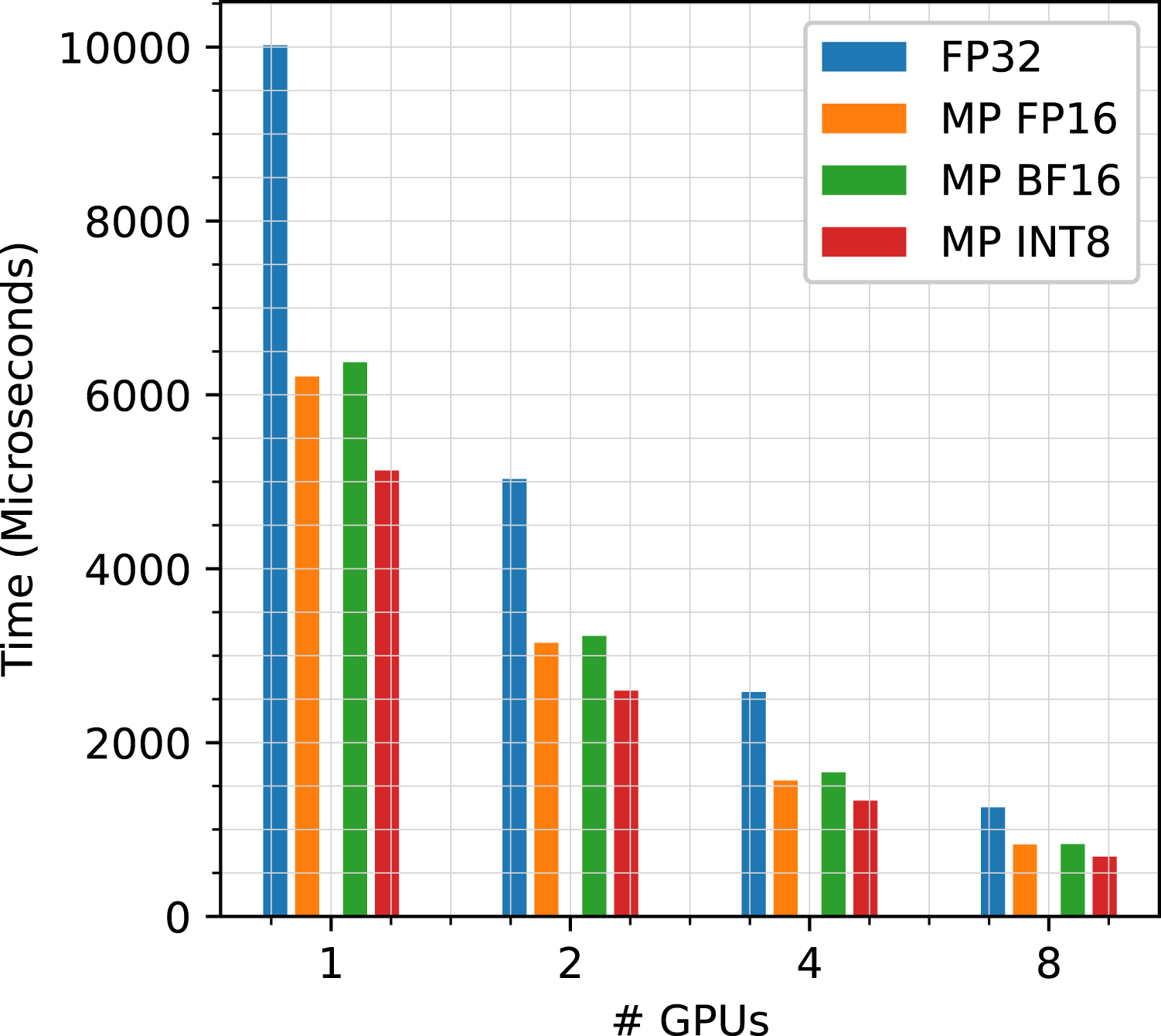

9.5. TLR-MVM performance on various architectures

Figure 18(a) and 18(b) show memory bandwidth and time to solution achieved by a single FP32 TLR-MVM on five different systems (see Table 1), respectively. The selected frequency matrix is a good proxy for the 150 matrices of our benchmark synthetic dataset, as described in Section 8. These two figures allow us to compare our TLR-MVM implementation against the traditional dense MVM kernel on various hardware architectures. On Rome, FP32 TLR-MVM with normal ordering scores more than an order of magnitude performance due to the high capacity of the Last-Level Cache (LLC), but also thanks to the proper MPI + OpenMP binding to map the processes/threads onto the underlying core complex (CCX) AMD packaging. Indeed, we launch 32 MPI processes with 4 OpenMP threads each that match the four cores per CCX sharing the same LLC and reach a throughput higher than the theoretical memory bandwidth. On ICX, our TLR-MVM with normal ordering saturates bandwidth compared to the dense MVM, since the compressed data of TLR-MVM is also now more amenable to fit into cache. The same observation applies to A64FX where our TLR-MVM benefits from cache effect along with HBM technology. On Aurora and A100, our TLR-MVM with normal ordering is able to take advantage of both specific architectures (i.e., long vector and SIMD), while also exploiting HBM. When we enable Hilbert ordering, additional performance gains can be noticed on all architectures in terms of time to solution, although the sustained bandwidth decreases for all except ICX. This is because TLR-MVM with Hilbert ordering creates even more opportunities for the kernel to fit into the cache of ICX, which engenders a throughput even higher than the theoretical memory bandwidth.

Figure 18.

Performance results comparison of a single frequency matrix (f = 33 Hz). (a) Memory bandwidth. (b) Time to solution. Red rectangles in (a) correspond to theoretical memory bandwidth on each system.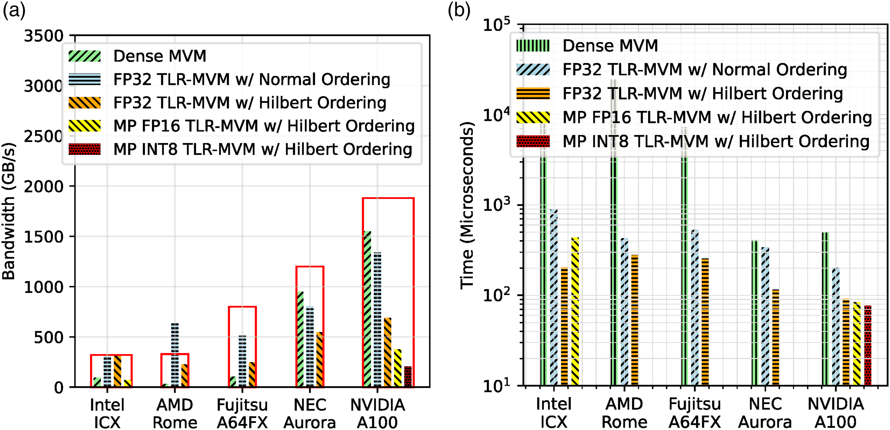

Finally, we made an attempt to develop MP variants of TLR-MVM for ICX and A64FX (not shown) since some levels of support are available. This means that we need to replace our memory-bound MVM kernel with the GEMM kernel that would operate on a single vector. As explained in Section 7.2.1, we achieve low performance compared to FP32 TLR-MVM on the respective hardware. We would need to have further support from vendors to reconsider these preliminary implementations in the future.

9.6. Overall performance of the application

To conclude, we present a short summary of the overall impact of MP TLR-MVM on the entire SRI algorithm. Following Ravasi and Vasconcelos (2021), we consider a scenario where we are interested to redatum the surface seismic data to a regular grid of size 41 × 71 covering an area of about 1.3 km² at a given subsurface depth. Figure 19 presents a time breakdown of the two phases involved in the entire SRI application. The compression phase is conducted on an Intel Ice Lake CPU cluster. We use 48 MPI processes, each with 12 cores. The rest of the workload—SFI framework is conducted on an A100 GPU. It is clear that the compression phase (blue bar) has a minimal overhead, also due to the embarrassingly parallel nature of this process. On the other hand, the actual redatuming process accounts for more than 90% of the overall time to solution; most of this time is actually spent in the various TLR-MVMs computations (orange bar), whilst the rest of the time is shared by the various FFTs (green bar) involved in the MDC operator and some vector-vector and vector-scalar operations in the LSQR solver (red bar). Note that if dense MVMs had been used here instead of MP TLR-MVMs, the overall time to solution would have further increased according to our findings in Figure 13.

Figure 19.

Time breakdown of SRI workflow in Ravasi and Vasconcelos (2021) after integrating MP INT8 TLR-MVM on one A100 GPU.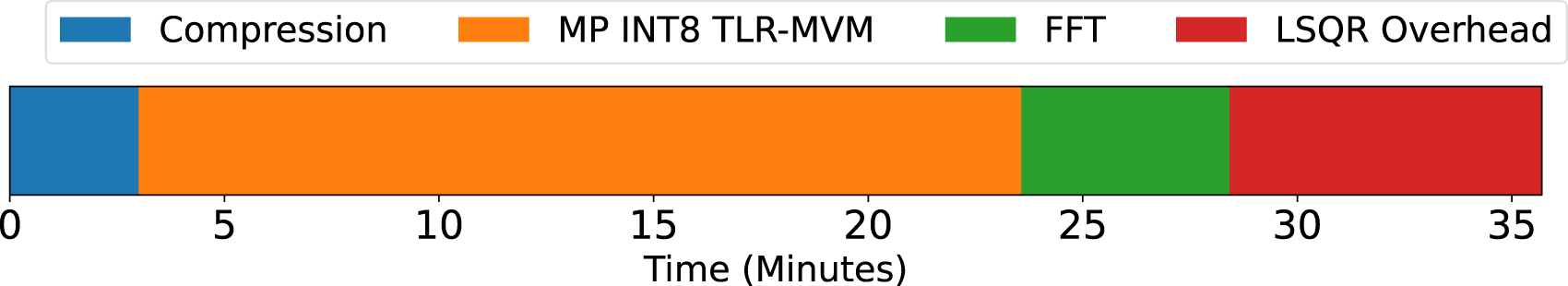

10. Conclusion

We present a novel high-performance implementation of the Multi-Dimensional Convolution operator using algebraic compression and mixed precisions, and employ it to efficiently solve the Seismic Redatuming by Inversion problem. Powered by Tile Low-Rank matrix approximations, we can accelerate the most time-consuming operations of the modeling operator, that is, the matrix-vector multiplications. Our TLR-MVM exploits the data sparsity in the frequency-space seismic data and permits to democratize large-scale SRI, otherwise industrially impractical due to large memory footprint and high algorithmic complexity. Additionally, we integrate two mixed-precision algorithms at the core of TLR-MVM to further improve the arithmetic intensity of the kernel. We achieve up to 63X memory footprint reduction and 12.5X performance speedup against the traditional dense MVM kernel on single NVIDIA A100 GPU using a realistic synthetic seismic dataset. Strong scalability is further attained when deploying our code on eight A100 GPUs. We also realize that standard hardware/software support from vendors is critical not only to extract performance but also to sustain code development. Vendor hardware/software roadmaps are mostly driven by AI workloads and it is important for traditional HPC to leverage these new features to remain in the exascale race. One example is the support for FP8 recently announced for the new NVIDIA Hopper GPU. This transformer-friendly precision arithmetic supported by hardware matrix engines may simplify our current INT8 implementations by removing the need for scaling, while revealing a yet more competitive approach. Finally, although this work has mainly targeted SRI from an application point of view, our findings have broader implications in the fields of geophysical processing, ultrasound processing, and medical imaging. In fact, any wave-equation-based processing algorithm that relies on the MDC operator will equally benefit from our novel implementation.

Footnotes

Acknowledgements

We are thankful to the Supercomputing Laboratory and the Extreme Computing Research Center at King Abdullah University of Science and Technology for their computing resources.

Declaration of conflicting interests

The author(s) declared no potential conflicts of interest with respect to the research, authorship, and/or publication of this article.

Funding

The author(s) disclosed receipt of the following financial support for the research, authorship, and/or publication of this article: The research reported in this paper was funded by King Abdullah University of Science and Technology.

ORCID iDs

Yuxi Hong

Hatem Ltaief

Author biographies

Yuxi Hong earned his PhD in Computer Science at King Abdullah University of Science and Technology (KAUST). He is now a post-doctoral fellow at Lawrence Berkeley National Laboratory. He received an MS degree in Electronics Engineering from Tsinghua University and a BSc from the Tsinghua University. His current research interests include High Performance Computing, Numerical Linear Algebra, GPU programming, HPC Applications Performance Optimization, Efficient Machine Learning/Deep learning.

Hatem Ltaief is the Princial Research Scientist in the Extreme Computing Research Center at KAUST, where is also advising several KAUST students in their MS and PhD research. His research interests include parallel numerical algorithms, parallel programming models, performance optimizations for many core architectures and high performance computing. He has contributed to the integration of numerical algorithms into mainstream vendors’ scientific libraries, such as NVIDIA cuBLAS and Cray LibSci. He has been collaborating with domain scientists, that is, astronomers, statisticians, computational chemists, and geophysicists, on leveraging their applications to meet the challenges at exascale. He received the engineering degree from Polytech Lyon at the University of Claude Bernard Lyon I in 2003, the MSc in applied mathematics in 2004 and the PhD degree in computer science at the University of Houston in 2008. Prior to joining KAUST, he held a research scientist position at the Innovative Computing Laboratory in Knoxville, TN USA.

Matteo Ravasi is an Assistant Professor at KAUST University in the Physical Science and Engineering division and head of the Deep Imaging Group. Previously, he worked in Equinor as both a research scientist and reservoir geophysicist. During his time in the industry, he contributed to the development of geophysical technologies aimed at identifying new discoveries as well as increasing hydrocarbon recovery of existing reservoirs. He has also been involved in the development of several open-source software packages to ease the use of geophysical data and improve reproducibility in the area of inverse problems. He earned a PhD in Geophysics from the University of Edinburgh as part of the Edinburgh Interferomety Project under the supervision of Prof. Andrew Curtis. His research contributions spanned across the fields of seismic processing, imaging, and inversion through the development of novel methods aimed at using high-order reverberations to improve the quality and resolution of subsurface imaging products.

David Keyes earned a BSE in aerospace and mechanical sciences from Princeton in 1978 and a PhD in applied mathematics from Harvard in 1984. He directs the Extreme Computing Research Center at KAUST. He works at the interface between parallel computing and the numerical analysis of PDEs, with a focus on scalable implicit solvers and exploiting data sparsity. He helped develop and popularize the Newton–Krylov–Schwarz (NKS) and Additive Schwarz Preconditioned Inexact Newton (ASPIN) methods. He has been awarded the ACM Gordon Bell Prize and the IEEE Sidney Fernbach Prize and is a fellow of the SIAM, AMS, and AAAS.

References

Abdelfattah

Anzt

Boman

, et al. (2021) A survey of numerical linear algebra methods utilizing mixed-precision arithmetic. The International Journal of High Performance Computing Applications 35(4): 344–369. DOI: 10.1177/10943420211003313.

Abdulah

Ltaief

Sun

, et al. (2018) Parallel approximation of the maximum likelihood estimation for the prediction of large-scale geostatistics simulations. In 2018 IEEE International Conference on Cluster Computing (CLUSTER), 98–108. DOI: 10.1109/CLUSTER.2018.00089.

Abdulah

Cao

Pei

, et al. (2022) Accelerating geostatistical modeling and prediction with mixed-precision computations: a high-productivity approach with PaRSEC. IEEE Transactions on Parallel and Distributed Systems 33(4): 964–976. DOI: 10.1109/TPDS.2021.3084071.

Akbudak

Ltaief

Mikhalev

, et al. (2017) Tile low rank Cholesky factorization for climate/weather modeling applications on manycore architectures. In 32nd International Conference on High Performance. Frankfurt, Germany: Springer, 22–40. ISBN 978-3-319-58667-0. DOI: 10.1007/978-3-319-58667-0_2.

Al-Harthi

Alomairy

Akbudak

, et al. (2020) Solving acoustic boundary integral equations using high performance tile low-rank LU factorization. In 35th International Conference on High Performance. Frankfurt, Germany: Springer. DOI: 10.1007/978-3-030-50743-5.

Alomairy

Bader

Ltaief

, et al. (2022) High-performance 3D unstructured mesh deformation using rank structured matrix computations. ACM Transactions on Parallel Computing 9(1): 1–23. DOI: 10.1145/3512756.

Ambikasaran

Foreman-Mackey

Greengard

, et al. (2015) Fast direct methods for Gaussian processes. IEEE Transactions on Pattern Analysis and Machine Intelligence 38(2): 252–265.

Amestoy

Ashcraft

Boiteau

, et al. (2015) Improving multifrontal methods by means of block low-rank representations. SIAM Journal on Scientific Computing 37(3): A1451–A1474. DOI: 10.1137/120903476.

Aminfar

Ambikasaran

Darve

(2016) A fast block low-rank dense solver with applications to finite-element matrices. Journal of Computational Physics 304: 170–188.

10.

Amundsen

(2001) Elimination of free‐surface related multiples without need of the source wavelet. Geophysics 66: 327–341. DOI: 10.1190/1.1444912.

11.

Börm

(2010) Efficient numerical methods for non-local operators: H2-matrix compression, algorithms and analysis. European Mathematical Society 14: 91.

12.

Börm

Grasedyck

Hackbusch

(2003) Introduction to hierarchical matrices with applications. Engineering Analysis with Boundary Elements 27(5): 405–422. DOI: 10.1016/S0955-7997(02)00152-2.

13.

Brackenhoff

Thorbecke

Koehne

, et al. (2021) 3D Marchenko applications: implementations and examples. Geophysical Prospecting, 70, 35–36.

14.

Broggini

Snieder

Wapenaar

(2012) Focusing the wavefield inside an unknown 1D medium: beyond seismic interferometry. Geophysics 77: A25–A28, A25–A28. DOI: 10.1190/geo2012-0060.1.

15.

Cao

Pei

Akbudak

, et al (2020) Extreme-scale task-based Cholesky factorization toward climate and weather prediction applications. In Proceedings of the Platform for Advanced Scientific Computing Conference (June 29 - July 1). ACM. DOI: 10.1145/3394277.3401846

16.

Cao

Abdulah

Alomairy

, et al (2022) Reshaping geostatistical modeling and prediction for extreme-scale environmental applications. In SC22: International Conference for High Performance Computing, Networking, Storage and Analysis, Dallas Texas, USA, 13 November-18 November 2022, DOI: 10.5555/3571885.3571888

17.

Cao

Pei

Akbudak

, et al. (2021) Leveraging PaRSEC runtime support to tackle challenging 3D data-sparse matrix problems. In 2021 IEEE International Parallel and Distributed Processing Symposium (IPDPS), Portland, OR, USA, May 17 2021–May 21 2021, 79–89. DOI: 10.1109/IPDPS49936.2021.00017.

18.

Charara

Keyes

Ltaief

(2018) Tile low-rank GEMM using batched operations on GPUs. In: Aldinucci

Padovani

Torquati

(eds). Euro-Par 2018: Parallel Processing, Turin, Italy: Springer, 811–825. ISBN 978-3-319-96983-1. DOI: 10.1007/978-3-319-96983-1_57

19.

Corona

Martinsson

Zorin

(2015) An O(N) direct solver for integral equations on the plane. Applied and Computational Harmonic Analysis 38(2): 284–317. DOI: 10.1016/j.acha.2014.04.002.

20.

Doucet

Ltaief

Gratadour

, et al. (2019) Mixed-precision tomographic reconstructor computations on hardware accelerators. In 2019 IEEE/ACM 9th Workshop on Irregular Applications: Architectures and Algorithms (IA3), Denver, CO, USA, 18 November 2019, 31–38.

21.

Dragoset

Verschuur

Moore

, et al. (2010) A Perspective on 3D surface-related multiple elimination. Geophysics 75: 75A245–75A261, 75A261. DOI: 10.1190/1.3475413.

22.

Fabien-Ouellet

(2020) Seismic modeling and inversion using half-precision floating-point numbers. Geophysics 85(3): F65–F76. DOI: 10.1190/geo2018-0760.1

23.

Flegar

Anzt

Cojean

, et al. (2021) Adaptive precision block-Jacobi for high performance preconditioning in the Ginkgo linear algebra software. ACM Transactions on Mathematical Software 47(2): 1–28. DOI: 10.1145/3441850.

24.

Goreinov

Tyrtyshnikov

Yeremin

(1997) Matrix-free iterative solution strategies for large dense linear systems. Numerical Linear Algebra with Applications 4(4): 273–294.

25.

Hackbusch

(1999) A sparse matrix arithmetic based on $\Cal H$ -matrices. Part I: Introduction to ${\Cal H}$ -matricesH-matrices. Part I: Introduction to H-matrices. Computing 62(2): 89–108. DOI:10.1007/s006070050015.

26.

Higham

Mary

(2022) Mixed precision algorithms in numerical linear algebra. Acta Numerica 31: 347–414. DOI: 10.1017/S0962492922000022.

27.

Hong

Ltaief

Ravasi

, et al. (2021) Accelerating seismic redatuming using tile low-rank approximations on NEC SX-Aurora TSUBASA. Supercomputing Frontiers and Innovations 31: 3. DOI: 10.14529/jsfi210201.

28.

IMF (2021) Reaching net zero emissions. URL. https://www.imf.org/external/np/g20/pdf/2021/062221.pdf.

29.

Joubert

Weighill

Kainer

, et al. (2018) Attacking the opioid epidemic: determining the epistatic and pleiotropic genetic architectures for chronic pain and opioid addiction. In SC18: International Conference for High Performance Computing, Networking, Storage and Analysis, Dallas Texas, USA, 11 November-16 November 2018, 717–730. DOI: 10.1109/SC.2018.00060.

30.

Jumah

Herrmann

(2012) Dimensionality-reduced estimation of primaries by sparse inversion. In SEG Technical Program Extended Abstracts, Denvor, CO, USA, 10 August-14 August 2012, 3520–3525. DOI: 10.1111/1365-2478.12113.

31.

Keyes

Ltaief

Turkiyyah

(2020) Hierarchical algorithms on hierarchical architectures. Philosophical transactions. Series A, Mathematical, physical, and engineering sciences 378(2166): 20190055. DOI: 10.1098/rsta.2019.0055.

32.

Kriemann

(2013) H-LU factorization on many-core systems. Computing and Visualization in Science 16(3): 105–117. DOI: 10.1007/s00791-014-0226-7.

33.

Becker

Ravasi

, et al. (2021) Closed-aperture unbounded acoustics experimentation using multidimensional deconvolution. Journal of the Acoustical Society of America 149(3): 1813–1828. DOI: 10.1121/10.0003706.

34.

Lindstrom

(2014) Fixed-rate compressed floating-point arrays. IEEE Transactions on Visualization and Computer Graphics 20(12): 2674–2683. DOI: 10.1109/TVCG.2014.2346458.

35.

Lopez*

Verschuur

(2015) 3D focal closed-loop SRME for shallow water. SEG Technical Program Expanded Abstracts 2015 203: 792–813. DOI: 10.1190/segam2015-5921009.1.

36.

Ltaief

Cranney

Gratadour

, et al. (2021) Meeting the real-time challenges of ground-based telescopes using low-rank matrix computations. In SC ’21: Proceedings of the International Conference for High Performance Computing, Networking, Storage and Analysis. ACM, St. Louis Missouri, USA, 14 November-19 November 2021, 1–16. DOI: 10.1145/3458817.3476225.

37.

Ltaief

Hong

Dabah

, et al. (2023a) Steering customized ai architectures for hpc scientific applications. In: Bhatele

Hammond

Baboulin

, et al. (eds). High Performance Computing. Cham: Springer Nature Switzerland, 125–143. ISBN 978-3-031-32041-5.

38.

Ltaief

Hong

Wilson

, et al. (2023b) Scaling the “memory wall” for multi-dimensional seismic processing with algebraic compression on cerebras cs-2 systems. In Proceedings of the International Conference for High Performance Computing, Networking, Storage and Analysis, SC ’23. New York, NY, USA: Association for Computing Machinery. ISBN 9798400701092. DOI: 10.1145/3581784.3627042.

39.

Ravasi

Vasconcelos

(2020) Pylops—a linear-operator python library for scalable algebra and optimization. SoftwareX 11: 100361.

40.

Ravasi

Vasconcelos

(2021) An open-source framework for the implementation of large-scale integral operators with flexible, modern high-performance computing solutions: enabling 3D Marchenko imaging by least-squares inversion. Geophysics 86: WC177–WC194. DOI: 10.1190/geo2020-0796.1.

41.

Ravasi

Vasconcelos

Kritski

, et al. (2016) Target-oriented Marchenko imaging of a North Sea field. Geophysical Journal International 205: 99–104. DOI: 10.1093/gji/ggv528.

42.

Ravasi

Hong

Ltaief

, et al. (2022) Large-scale Marchenko imaging with distance-aware matrix reordering, tile low-rank compression and mixed-precision computations. Second International Meeting for Applied Geoscience & Energy 5: 9. DOI: 10.1190/image2022-3744978.1.

43.

Rouet

Ghysels

, et al. (2016) A distributed-memory package for dense hierarchically semi-separable matrix computations using randomization. ACM Transactions on Mathematical Software 42(4): 1–35. DOI: 10.1145/2930660.

44.

van der Neut

Thorbecke

Wapenaar

, et al. (2015) Inversion of the multidimensional Marchenko equation. In 77th Conference and Exhibition, EAGE, Extended Abstracts, Madrid, Spain, 1 June-4 June 2015. DOI: 10.3997/2214-4609.201412939.

45.

van Groenestijn

Verschuur

(2009) Estimating primaries by sparse inversion and application to near-offset data reconstruction. Geophysics 74: A23–A28, 1MJ–Z54. DOI: 10.1190/1.3111115.

46.

Wapenaar

Thorbecke

van der Neut

, et al. (2014) Marchenko imaging. Geophysics 79: WA39–WA57. DOI: 10.1190/geo2013-0302.1.

High performance computing seismic redatuming by inversion with algebraic compression and multiple precisions

Abstract

Keywords

1. Introduction

2. Related work

3. Contributions

4. Marchenko-based SRI

5. Powering SRI using TLR-MVM

5.1. TLR data compression format

5.2. Impact of matrix reordering

5.3. Impact on SRI computational stages

6. Mixed-precision TLR-MVM computations

7. Implementation details

7.1. Extending TLR-MVM portability to other systems

7.2. Mixed-precision TLR-MVM

7.2.1. Hardware/software limitations for mixed precisions

7.2.2. MP TLR-MVM using FP16/FP32

7.2.2.1. Vectorized global memory access

7.2.2.2. Warp-level reduction

7.2.3. MP TLR-MVM using INT8/INT32/FP16/FP32

8. Numerical accuracy

9. Performance analysis

9.1. Environment settings

9.2. Performance impact of GPU streams on TLR-MVM

9.3. Impact of matrix reordering and MP on TLR-MVM

9.4. Performance scalability and roofline of MP TLR-MVM

9.5. TLR-MVM performance on various architectures

9.6. Overall performance of the application

10. Conclusion

Footnotes

Acknowledgements

Declaration of conflicting interests

Funding

ORCID iDs

Author biographies

References