Sage Journals: Discover world-class research

Abstract

Fluid dynamics is a ubiquitous problem that arises in different branches of science and industry. It is usually tackled by numerically solving continuum Navier-Stokes type equations. Molecular dynamics has been not a feasible tool to approach fluid dynamics until very recently due to its disproportional computational complexity for relevant system sizes. In this paper, we propose a new type of boundary conditions for molecular dynamics simulations of stationary fluid flows and present its possible GPU-based implementations in OpenMM and LAMMPS. We examine the performance and scalability of the proposed implementations. The benchmarking results show promising performance that makes it possible to reach turbulence in atomistic models of stationary fluid flows using modern supercomputers.

Keywords

molecular dynamics fluid flows GPU computing OpenMM LAMMPS Kokkos performance portability

1. Introduction

For the numerical study of laminar and turbulent fluid flows, the generally accepted method of their simulation is numerical solution of the Navier-Stokes equations. Attempts to numerically solve the Navier-Stokes equations date back to the very dawn of the computer era (Kawaguti (1953); de G. Allen and Southwell (1955); Simuni (1964); Chorin (1968)). Since then this approach and its different variations have remained dominant.

Unfortunately, Navier-Stokes equations have fundamental limitations, since the premise that the system can be represented as a continuous field does not hold at the atomistic scale where many important physical processes take place, see e.g. Hadjiconstantinou (2006); Grinberg et al. (2011); Sergeenko et al. (2022). The onset of turbulence is always analysed as a multiscale phenomenon (e.g. see Chashechkin and Mitkin (2001)) and its fundamental understanding in fluid flows should include the atomistic level description at the Kolmogorov’s length scale (Kolmogorov (1941)). The development of high performance computing systems brings the promise that such an atomistic-level description of turbulent fluid flows will come true, and in this paper, we describe our step to this goal.

Classical molecular dynamics (MD) simulation method is a key research tool in many areas of science and engineering. Nowadays MD is one of the major consumers of supercomputer resources worldwide. MD tools that enable ultra-long MD trajectories (up to tens of milliseconds) and extreme MD system sizes (up to trillions of atoms) are important avenues of development for high performance computing methods (Begau and Sutmann (2015); Tchipev et al. (2019); Shaw et al. (2021)). Shortly after the Nvidia CUDA technology had been introduced in 2007, hybrid MD algorithms that use GPU accelerators appeared and showed their promising performance. Currently, GPU-accelerated hardware provides the most efficient and affordable way of doing MD studies as shown in Kutzner et al. (2015, 2019); Stegailov et al. (2019); Kondratyuk et al. (2021) and makes various applied MD studies feasible, e.g. see Nikolskiy and Stegailov (2020); Nguyen-Cong et al. (2021); Antropov and Stegailov (2023); Fominykh et al. (2023); Kondratyuk et al. (2023).

The emergence of parallel distributed memory supercomputing systems stimulated the development of parallel algorithms for MD calculations. Among others, LAMMPS (Thompson et al. (2022)) is an MD package that has developed into a versatile simulation MD toolkit and is widely used nowadays on high performance computing systems. Since the emergence of general-purpose computing on graphics processing units (GPGPU), LAMMPS has been supplemented with GPU offloading capabilities as described in Brown et al. (2011, 2012); Brown and Yamada (2013). Newer MD libraries like HOOMD (Anderson et al. (2008); Glaser et al. (2015)) and OpenMM (Eastman et al. (2013, 2017)) use GPU-oriented MD algorithms that are designed in a way that keeps the amount of CPU-GPU communication to an absolute minimum. This is also a feature of the Kokkos-based variant of LAMMPS (Thompson et al. (2022)) aimed at performance portability, GPU acceleration including.

In this work, we extend our preliminary results (Pavlov et al. (2023)) on the novel kind of boundary conditions for MD of fluid flows, demonstrate a working OpenMM and LAMMPS/Kokkos implementations of such boundary conditions and compare the performance of OpenMM and LAMMPS/Kokkos for very large system sizes.

2. Related work

The first attempts to apply MD for studying eddy formation in fluid flows were carried out by Rapaport and Clementi (1986) in a two-dimensional system and for a small (according to modern standards) number of particles (N ≈ 10⁴). With the rise of supercomputing capabilities in 2000s, MD calculations at extreme length scales were considered in Kadau et al. (2010) as a tool that is able to complement Navier-Stokes-based continuum fluid-simulation methods. MD models revealed the influence of the wall-fluid interactions on slip flow of simple fluids Priezjev (2007) and the structure of oscillatory Couette flows Priezjev (2013). A special MD package ls1 mardyn focused on extreme length scales is under development (Tchipev et al. (2019)) and is being used for the corresponding multiscale simulations (Hitz et al. (2020, 2021)).

Among the most remarkable results published recently we would mention the work of Komatsu et al. (2014) and the work of Smith (2015) that compare MD and Navier-Stokes descriptions of special turbulent flow patterns. Smith (2015) provides the detailed description of MD modelling using the SGI Altix ICE 8200 EX supercomputer with manycore CPUs and Infiniband interconnect. Below, we compare the data of Smith (2015) with our MD calculations for a similar fluid using modern multi-GPU systems.

The coupling between CFD and MD algorithms is under active development: for example, Grinberg et al. (2011) discuss the coupling of Navier-Stokes equations with particle-based models. Smith et al. (2020) described such a coupling for OpenFOAM and LAMMPS. A multiscale 3D model based on the dissipative particle dynamics with special inflow/outflow boundary conditions was implemented in LAMMPS for blood flow simulations by Lykov et al. (2015).

The success of using Kokkos library for performance portable code development aimed at molecular dynamics is exemplified by LAMMPS and other projects, e.g. the recent work on Multi-Particle Collision Dynamics of Halver et al. (2023).

3. Software

As a part of this work, we implemented a new kind of boundary conditions using the OpenMM and LAMMPS packages. Below, we describe both packages briefly.

3.1. OpenMM

OpenMM (Eastman et al. (2017)) is an open source toolkit for molecular dynamics. With its main focus being computational biology, it still performs remarkably well on other systems. This is achieved because unlike the high-level OpenMM Application Layer Python API OpenMM team, 2023a, which is built around domain-specific constructs such as force fields, residue chains and topologies, OpenMM Library Level C++/Python API OpenMM team, 2023b is completely divorced from such constructs and provides a lower-level access to the underlying structures that can be used in a broader range of applications.

OpenMM supports four platforms: Reference, CPU, CUDA, OpenCL. There also exists a separately-developed plugin StreamHPC (2023) that adds HIP support to the list. CUDA, HIP and OpenCL are GPU-oriented platforms, and they provide the best performance when compared to the CPU and Reference platforms which don’t use GPU acceleration. The underlying algorithms that are used in these platforms are almost identical, with most of the code having been merged into a meta-platform called Common Compute. CUDA, OpenCL and HIP platforms operate in mostly the same way.

When parallelizing over a big amount of processing units, there are three wide classes of approaches as described by Plimpton (1995): atom-decomposition, force-decomposition and domain-decomposition. For distributing workload inside a GPU, OpenMM uses a force-decomposition-like algorithm as described in Eastman and Pande (2009): for N atoms, the NxN force matrix is divided into ‘tiles’ of size 32x32. Then, only the tiles that might contain non-zero forces are marked as ‘interacting’ based on comparing the tiles’ coordinate bounds. Then, the list of interacting tiles is traversed to calculate forces and energy. Once the tiles’ bounds change to a point that new interactions might appear, the list of interacting tiles is rebuilt.

One serious downside of this algorithm is its complexity: traversing an NxN force matrix has the complexity of $O (N^{2})$ . This means that this algorithm is not infinitely scalable: at some point the rapidly increasing cost of finding interacting tiles would outweigh the benefits of being able to simulate bigger systems. The question is how soon.

3.2. LAMMPS

LAMMPS is an open-source package for classical molecular dynamics computations written in C++. It is designed to be compiled and run on local computers as well as on supercomputers, and allows the simulation of many millions of particles. It implements a large number of models of interaction potentials, ranging from the most popular to very rare ones.

The source code of LAMMPS is very extensible, allowing both very easy addition of new interaction potentials and fine-tuning of the numerical integration process by making changes to individual steps. The latter is achieved with the help of a so-called “fix” mechanism (Thompson et al. (2022)).

To optimize the computation of the short-range potential, LAMMPS implements domain decomposition: it splits the simulation box into sub-domains (one per MPI rank) and distributes the computation for atoms within all of them. Moreover, LAMMPS creates Verlet neighbor list (Eijkhout et al., 2016, ch. 7.1.2) for each particle inside the sub-domains which stores atoms near that particle within radius r_c. For even more optimization, LAMMPS uses the same list at multiple time steps, and the clipping radius is increased to r_v = r_c + 2nd, where d is the estimated maximum distance a particle can travel in a time step, and n is the number of steps at which the neighbor lists are updated. To perform neighbour list construction in linear time, LAMMPS bins each sub-domain’s particles into a uniform cell grid (this is known as the linked cell method). Applying both of these optimizations when calculating the short-range potential yields the asymptotic complexity of $O (N \cdot N_{a})$ , where N is the number of atoms, and N_a is the average number of atoms within the cutoff, which makes LAMMPS excellently scalable, and gives us the ability to move to even larger systems. One disadvantage of using Verlet neighbor lists is that we have to use extra memory, which one could also asymptotically estimate as $O (N \cdot N_{a})$ . Moreover, the use of partitioning into sub-domains entails the need to exchange atoms between processes when an atom moves from one sub-domain to another, leading to a drop in performance, as we also demonstrate in the results of our experiments.

LAMMPS is also capable of optimizing the computation of long-range potentials, either using FFT or the multipole method, but we have not used the long-range potential in our simulations.

The general support of heterogeneous computing in LAMMPS is based on the Kokkos library, which allows writing performance-portable code and is designed for almost all existing supercomputer systems (Edwards et al. (2014)). To use it, you can write the code once, and then you just have to specify the required target platforms in compilation flags. The Kokkos library is integrated into the LAMMPS package as the Kokkos module. In addition to this module in LAMMPS, there is another older module called GPU that uses an offload strategy of GPU acceleration. One can anticipate that LAMMPS/Kokkos will perform better on modern DGX-like GPU servers due to less amount of data transfers between CPUs and GPUs.

4. Flow Boundary Conditions

When running MD simulations, it is not feasible and currently not possible to simulate a macroscopic system due to its enormous amount of particles. So it is common practice to simulate a small system as a part of the whole by putting it in periodic boundary conditions (PBC). However, if one was to simulate a fluid flow using just the PBC, the collective kinetic energy of the flow would dissipate over time, eventually bringing the flow to a halt. In real-world scenarios, whenever there is a stationary flow of some kind, there is also an energy source that keeps pumping kinetic energy into the system to counteract this energy dissipation. This means that a simple NVE simulation with PBC is unfit for these kinds of models.

This problem can be addressed in a number of ways: for example, by introducing moving walls to create a Couette flow (like in Smith (2015)), or by reintroducing particles that left the cell with a reset velocity (like in Rapaport and Clementi (1986)). In this paper, we expand upon the latter method. The Flow Boundary Conditions (FBC) that we introduce are a special kind of boundary conditions that resembles PBC, but resets particle velocities whenever they cross one of the periodic boundaries.

4.1. Derivation of Flow Boundary Conditions for an ideal gas

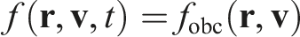
For simplicity, we assume that all particles in the system are identical, and that the system is an ideal gas. Let us consider the Boltzmann equation for a single-particle probability density function f (r, v, t):

\frac{\partial f}{\partial t} + v \cdot \frac{\partial f}{\partial r} + \frac{F_{ext}}{m} \cdot \frac{\partial f}{\partial v} = {\frac{\partial f}{\partial t} |}_{coll}

Here, m, r and v are the mass, the position, and the velocity of a particle respectively, t is time, and F_ext is the external force applied to the particle.

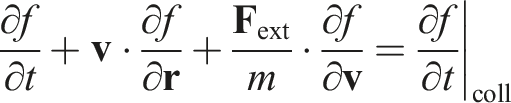
We wish to create a stationary flow by using some sort of boundary conditions. Since the flow is stationary, the desired probability density function f_obc is also stationary, so

f (r, v, t) = f_{obc} (r, v)

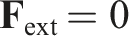
Also, there are no external forces, therefore

F_{ext} = 0

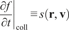
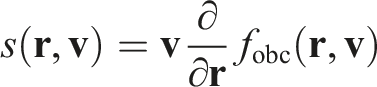
The right-hand side of the equation represents the collision term. It would normally represent changes in the probability density function due to particle collisions. However, since we assume that the gas is ideal, the collision term represents only the particle interactions with FBC. The analytical form of this term shall dictate the exact behavior of FBC. Let us denote it as s (r, v):

{\frac{\partial f}{\partial t} |}_{coll} \equiv s (r, v)

Then, by substituting all of the above into the initial Boltzmann equation, we get

s (r, v) = v \frac{\partial}{\partial r} f_{obc} (r, v)

Let us say we want to simulate a part of an infinite stationary flow that has the probability density function f(v).

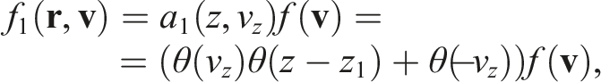
Let us assume the left-side boundary is situated at the plane z = z₁. Particles to the left of the boundary are not simulated directly, but their impact must be somehow approximated. We can outline two kinds of impact that these particles make: first, they interact with particles on the right side, and second, the left and the right side exchange particles. The former impact is sufficiently approximated by PBC. The latter one, however, is not: in the case with stationary fluid flow, it is impossible to maintain the pressure gradient with just PBC. The solution we propose is to make FBC emit particles into the right side of the left-side boundary, instead of them naturally coming from the left side (and vice versa for the right side). To do this on the left side, we want to remove all particles with z < z₁ and v_z > 0 from the initial probability density function f(v), while preserving it where z > z₁.

f_{1} (r, v) = {\begin{cases} 0, z < z_{1}, v_{z} > 0, \\ f (v), z < z_{1}, v_{z} < 0, \\ f (v), z > z_{1} . \end{cases}

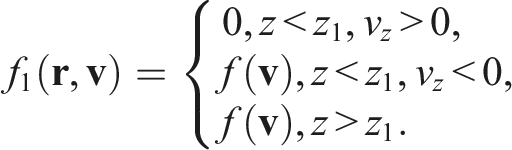
It could be achieved by multiplying the initial distribution by some a₁ (z, v_z):

\begin{array}{l} f_{1} (r, v) = a_{1} (z, v_{z}) f (v) = \\ = (θ (v_{z}) θ (z - z_{1}) + θ (- v_{z})) f (v), \end{array}

where θ is the Heaviside step function.

By analogy, for the right-side boundary we can define a₂ (z, v_z):

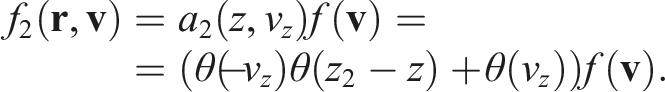
\begin{array}{l} f_{2} (r, v) = a_{2} (z, v_{z}) f (v) = \\ = (θ (- v_{z}) θ (z_{2} - z) + θ (v_{z})) f (v) . \end{array}

By multiplying the initial distribution f(v) by both a₁ (z, v_z) and a₂ (z, v_z), we will get a sector z₁ < z < z₂ where all particles that come inside are emitted by FBC:

f_{obc} (r, v) = a_{1} (z, v_{z}) a_{2} (z, v_{z}) f (v)

and then

\begin{array}{l} s (r, v) = v \cdot \frac{\partial}{\partial r} f_{obc} (r, v) = \\ = v \cdot \frac{\partial}{\partial r} (a_{1} (z, v_{z}) a_{2} (z, v_{z}) f (v)) . \end{array}

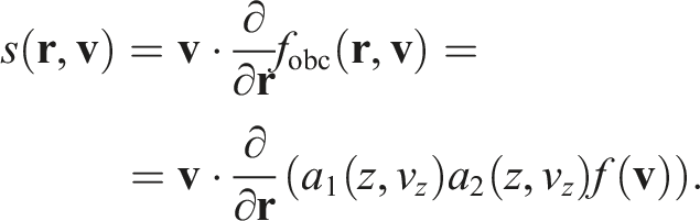
It is worth noting that $a_{1} (z, v_{z}) \frac{\partial}{\partial z} a_{2} (z, v_{z}) = \frac{\partial}{\partial z} a_{2} (z, v_{z})$ and $a_{2} (z, v_{z}) \frac{\partial}{\partial z} a_{1} (z, v_{z}) = \frac{\partial}{\partial z} a_{1} (z, v_{z})$ for any z, v_z, when z₁ < z₂.

Then, finally,

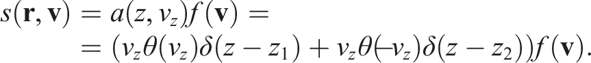
\begin{array}{l} s (r, v) = a (z, v_{z}) f (v) = \\ = (v_{z} θ (v_{z}) δ (z - z_{1}) + v_{z} θ (- v_{z}) δ (z - z_{2})) f (v) . \end{array}

The resulting distribution f_obc (r, v) fully matches f(v) in the z₁ < z < z₂ sector that we are modelling. In other words, if we are considering the part of the system that is inside this sector, there is no observable difference between a system that follows the f_obc (r, v) distribution or the f(v) distribution.

4.2. Flow Boundary Conditions algorithm

The nature of the collision term $a (z, v_{z}) f (v) = s (r, v) =$ dictates how often, on which side and with what velocity particles are emitted. Our implementation does not change the amount of particles in the system, it only resets their velocities when they hit the boundary, effectively re-emitting them from an appropriate side with an appropriate velocity, according to the distribution. There is an emergent property that since the flow is stationary, the amount of particles that leave the sector z₁ < z < z₂ equals the amount that is emitted. It eliminates the need to change the amount of particles over the course of the simulation.

The first step of the algorithm is detecting which particles crossed the border. The simplest way to do it is by iterating over every particle and checking whether or not this event occurred. Once a particle crosses the border, the first thing that needs to be computed is which side it should be re-emitted on (the possibility of the particle being re-emitted is one of the distinguishing traits of our approach; it was not accounted for by Rapaport and Clementi (1986)). The probability of a particle being re-emitted from a certain side can be derived as follows:

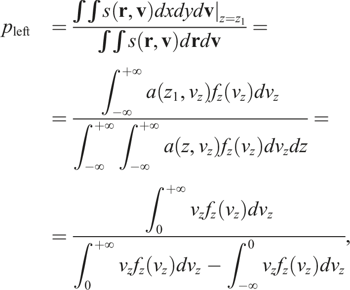
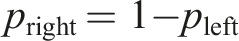
\begin{array}{l} p_{left} & = \frac{{\iint \iint s (r, v) d x d y d v |}_{z = z_{1}}}{\iint \iint s (r, v) d r d v} = \\ = \frac{\int_{- \infty}^{+ \infty} a (z_{1}, v_{z}) f_{z} (v_{z}) d v_{z}}{\int_{- \infty}^{+ \infty} \int_{- \infty}^{+ \infty} a (z, v_{z}) f_{z} (v_{z}) d v_{z} d z} = \\ = \frac{\int_{0}^{+ \infty} v_{z} f_{z} (v_{z}) d v_{z}}{\int_{0}^{+ \infty} v_{z} f_{z} (v_{z}) d v_{z} - \int_{- \infty}^{0} v_{z} f_{z} (v_{z}) d v_{z}}, \end{array}

p_{right} = 1 - p_{left}

It is worth noticing that the above formula is agnostic to whether the particle left the cell upstream or downstream. In practice, due to the periodic conditions, the re-emission of a particle does not actually require its position to be changed. The re-emission is effectively just a re-assignment of velocity without any necessary modification to the particle position. Since such a mechanism can be represented as a plane that changes the velocity of any particle that passes through, there is no need to even introduce any extra ghost atoms.

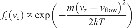
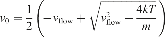
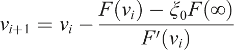
From now on, let us assume that the particle is emitted from the left side. The new velocities on x and y need only be picked from f_x(x) and f_y(y) distributions (which are just Maxwell distributions in our case). The v_z can be inferred from the following equation, where ξ₀ ∈ (0, 1) is a uniformly-distributed random number:

ξ_{0} F (\infty) = F (v_{z})

where

\begin{array}{l} F (v_{z}) = {\iint s (r, v^{'}) d x d y d v^{'} |}_{z = z_{1}, v_{z}^{'} < v_{z}} = \\ = \int_{0}^{v_{z}} v_{z}^{'} f_{z} (v_{z}^{'}) d v_{z}^{'} . \end{array}

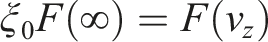
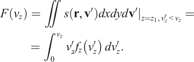
Now, we want the underlying distribution f(v) to be a shifted Maxwell distribution:

f_{z} (v_{z}) \propto \exp (- \frac{m {(v_{z} - v_{flow})}^{2}}{2 k T})

Then F (v_z) can be computed in terms of error functions, allowing us to solve the equation numerically. We use the Newton’s method to find the root of the equation. From now on, v_i is the ith approximation on the velocity v_z:

v_{i + 1} = v_{i} - \frac{F (v_{i}) - ξ_{0} F (\infty)}{F^{'} (v_{i})}

In our case, the F(v) is a monotonic function with a single inflection point on (0, + ∞), and F′(0) = F′(+∞) = 0. Therefore the best starting point for the Newton’s method to avoid oscillation and guarantee convergence would be that inflection point:

v_{0} = \frac{1}{2} (- v_{flow} + \sqrt{v_{flow}^{2} + \frac{4 k T}{m}})

4.3. OpenMM implementation

The OpenMM implementation of the FBC (Pavlov, 2022a; Pavlov et al., 2023) was our earlier attempt in implementing the aforementioned algorithm. It was implemented as the OpenBoundary class that extends the Force abstract class. It is currently implemented for the Common Compute platform only (which makes it possible to run it using GPU-oriented platforms such as CUDA, OpenCL, or HIP) and it performs the bulk of its calculations on the GPU.

The OpenMM implementation also supports having multiple FBC planes inside the simulation box (see the discussion below). Additionally, it supports having no additional internal planes with only the box boundary acting as an FBC plane.

Currently, the master branch of OpenMM uses 32-bit counters for storing tile indices. This makes it impossible to correctly run systems bigger than $\sim 30$ million atoms. However, we have created a patch (Pavlov, 2022b) to change the counters to 64-bit. This allows benchmarking bigger systems. Current GPU memory limitations restrict the use of OpenMM to systems with up to 10⁷ − 10⁸ atoms.

4.4. LAMMPS implementation

We have created a new fix called fix wall/flow (Galigerov, 2023). Another option we considered was to create a new boundary style. Boundary styles determine which boundary conditions LAMMPS applies to atoms near the edges of the simulation domain: periodic, shrink-wrapped, or fixed. As it is discussed below, using only one plane on which we reset particle velocities (we call these planes walls in the LAMMPS implementation) might not be sufficient, so we might have to create several such planes inside the simulation volume. From this point of view, our planes, which model Flow Boundary Conditions, are to some extent “walls” reassigning particle velocities, rather than “boundaries”, so we rejected the idea of adding a new boundary style.

The walls divide the simulation box along some axis into segments. In order to keep track of the events of an atom crossing a wall, our algorithm checks the segment index from the previous step and compares it to the current segment index. To keep track of the segment index, we have added a per-atom index array in this fix. This array is also involved in exchanging atom data between MPI processes, and for now there seems to be no apparent way to avoid this extra work.

The syntax of our fix is:

fix ID group - ID wall / flow args . . .

where ID is the user-defined name of the fix, group-ID is the name of the group to which the user wants to apply the fix, wall/flow is just the name of the fix. The args… part are the arguments that go as follows:

ax vf T seed N coords \dots

where ax is the flow axis (x, y, or z character), vf > 0 is ax component of flow velocity, T is the temperature, seed is the random number generator seed, N >= 1 is the number of walls and coords… is a set of the N coordinates of walls perpendicular to the chosen axis. Note that we insert an additional implicit wall on the simulation domain boundary, so as the result we always have N+1 walls. We have done this to avoid ambiguity in the computation of the atom’s current segment index.

The fix gets the flow direction from the sign of vf (but it is important to note that the fix currently works for vf > 0) only.

4.5.1. Kokkos-accelerated version

We also have implemented a Kokkos version of this fix in LAMMPS. In general, its idea and structure is exactly the same as the regular version, which is what Kokkos is designed to do.

However, there was a pitfall worth mentioning. Before the 22 August 2023 release, LAMMPS was not able to use GPU-aware MPI capabilities to exchange data when there is at least one Kokkos-accelerated fix that needs to communicate data. In that case, LAMMPS disabled GPU-aware MPI and exchanged all data (including per-atom arrays that are not part of the fix) through the host. As we said above, our fix contains an additional per-atom array, which participates in the exchange between processes. Fortunately, there is a Pull Request (Taniguchi (2019)) that has been merged recently, which allowed us to optimize away the need to copy data to host and back when a direct communication between GPUs is possible. The LAMMPS/Kokkos benchmark results presented in this paper have been obtained with this new capability.

5. Grid aggregation

When processing trajectory data from simulations, it is not always feasible to process it on per-particle basis, and some kind aggregation is necessary. Here, we calculate average velocities on a grid of N_cells = N_x × N_y × N_z cells.

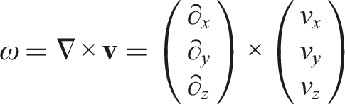
One of the principal metrics in analyzing fluid flows is vorticity:

ω = \nabla \times v = (\begin{array}{l} \partial_{x} \\ \partial_{y} \\ \partial_{z} \end{array}) \times (\begin{array}{l} v_{x} \\ v_{y} \\ v_{z} \end{array})

Then, by abuse of notation, we can derive a numerical approximation of vorticity for our grid:

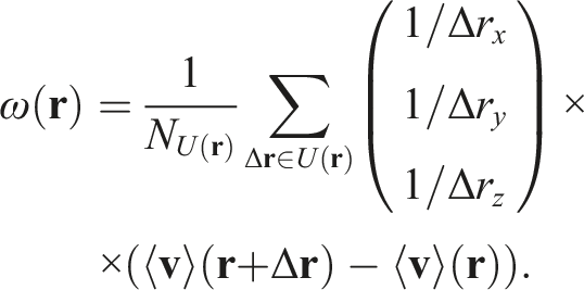
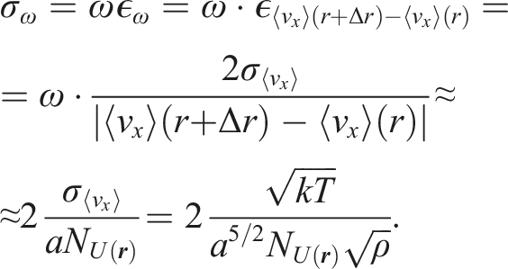
\begin{array}{l} ω (r) = \frac{1}{N_{U (r)}} \sum_{Δ r \in U (r)} (\begin{array}{l} 1 / Δ r_{x} \\ 1 / Δ r_{y} \\ 1 / Δ r_{z} \end{array}) \times \\ \times (〈 v 〉 (r + Δ r) - 〈 v 〉 (r)) . \end{array}

Here U(r) is a set of offsets of neighboring grid cells, N_U(r) is the number of such cells and ⟨v⟩(r) is the space-averaged velocity within the cell with its center at r. One important part is to exclude the terms where Δr_i = 0 from the average to avoid infinite results.

However, the images obtained using this approximation can be noisy. Indeed, it is not always correct to assume that it is possible to measure a continuous field of values on an atomic level. The next step is quantifying errors of values obtained from averaging on grid cells. We use σ to denote the absolute error of a value and ϵ to denote its relative error.

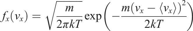
The single-axis Maxwell velocity distribution is:

f_{x} (v_{x}) = \sqrt{\frac{m}{2 π k T}} \exp (- \frac{m {(v_{x} - 〈 v_{x} 〉)}^{2}}{2 k T})

and if there is N particles in total spread over the total of N_cells cells with a side of a, then the standard error of velocity, averaged over one cell is

\begin{array}{l} σ_{〈 v_{x} 〉} = \sqrt{\frac{σ_{v_{x}}^{2}}{N / N_{cells}}} = \sqrt{\frac{N_{cells}}{N} \cdot \frac{k T}{m}} = \\ = \sqrt{\frac{1}{a^{3}} \cdot \frac{k T}{ρ}} = \sqrt{\frac{k T}{m_{cell}}} . \end{array}

When approximating the error of vorticity, the following approximation might be useful:

〈 v 〉 (r + Δ r) - 〈 v 〉 (r) \approx ω a N_{U (r)}

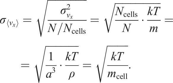
Now, the error of vorticity is:

\begin{array}{l} σ_{ω} = ω ϵ_{ω} = ω \cdot ϵ_{〈 v_{x} 〉 (r + Δ r) - 〈 v_{x} 〉 (r)} = \\ = ω \cdot \frac{2 σ_{〈 v_{x} 〉}}{| 〈 v_{x} 〉 (r + Δ r) - 〈 v_{x} 〉 (r) |} \approx \\ \approx 2 \frac{σ_{〈 v_{x} 〉}}{a N_{U (r)}} = 2 \frac{\sqrt{k T}}{a^{5 / 2} N_{U (r)} \sqrt{ρ}} . \end{array}

5.1. Distributed grids aggregation in LAMMPS

Since the 22 December 2022 release LAMMPS has a special mechanism called distributed grids. They consist of uniformly distributed cells covering the simulation box. There are also commands that utilize these grids to perform different operations.

To perform grid aggregation we have used such a distributed grids mechanism with different cell resolutions and the fix ave/grid command. Data obtained this way has later been used for vorticity and density distribution computations. The fix ave/grid command allows for averaging grid data over time, however this functionality has not been used in this work, as we have used only spacial averaging.

6. Simulation results

6.1. Performance comparison

The analysis presented in this work is based on the data obtained using two multi-GPU systems: the Desmos supercomputer (Stegailov et al. (2019); Shamsutdinov et al. (2021)) with 32 single-GPU nodes equipped with AMD MI50 GPUs and connected via Infiniband FDR (that works with the mlnx_ofed driver ver. 4.9), and a single node of the cHARISMa supercomputer (Kostenetskiy et al. (2021)) with 8 Nvidia A100 GPUs connected via NVLink (see Table 1). The runtimes used are AMD ROCm ver. 5.3.3 for MI50 and NVIDIA HPC SDK ver. 22.7 with CUDA ver. 11.7 for A100.

Table 1.

Specifications of the multi-GPU systems considered in this work.

	Desmos	cHARISMa
Number of nodes	1-32	1
GPUs per node	1 AMD MI50	8 Nvidia A100
GPU memory	32 GB	80 GB
GPU memory BW	1 TB/s	2 TB/s
GPU FP32 perf.	13.3 TFLOPS	19.5 TFLOPS
GPU FP64 perf.	6.6 TFLOPS	9.7 TFLOPS
Interconnect	FDR	NVLink
GPU-aware MPI	OpenMPI 5.0	OpenMPI 4.1

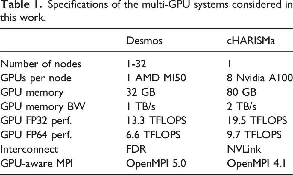
OpenMM and LAMMPS are built in the “Release mode”. Precision is set to mixed in OpenMM, and to double in LAMMPS/Kokkos (due to the fact that the mixed precision is not supported by LAMMPS/Kokkos).

The systems that we are running benchmarks on are LJ systems with the main parameters borrowed from Smith (2015) unless specified otherwise. Those systems have the relative dimensions of approximately 10:2:1 with a cylindrical obstacle in the upstream part.

We have measured the performance of both our FBC implementation in OpenMM and our Kokkos accelerated LAMMPS implementation of fix wall/flow as shown in Figure 1. It can be seen that OpenMM’s performance suffers severely as the number of atoms exceeds N ≈ 10⁶. This illustrates how OpenMM is bound by $O (N^{2})$ complexity. Such big systems lie outside the usual scope of OpenMM simulations with its main focus being attaining better performance for small and medium-sized systems. The presence of FBC introduces a slowdown factor that is increasing along with the amount of atoms, whereas the performance of the LAMMPS/Kokkos implementation remains near-constant.

Figure 1.

Benchmark results for the Lennard-Jones fluid. The performance of MD calculations is shown as N_atoms · N_steps per unit of wall-clock time (higher is better). Results for A100 and MI50 GPUs are presented. The rhombs show the data for OpenMM, the dots show the data for Kokkos backend of LAMMPS on MI50 and A100 GPUs. The performance of 256 Intel Xeon Nehalem cores used in Smith (2015) for a 300 million atom simulation is shown as a star.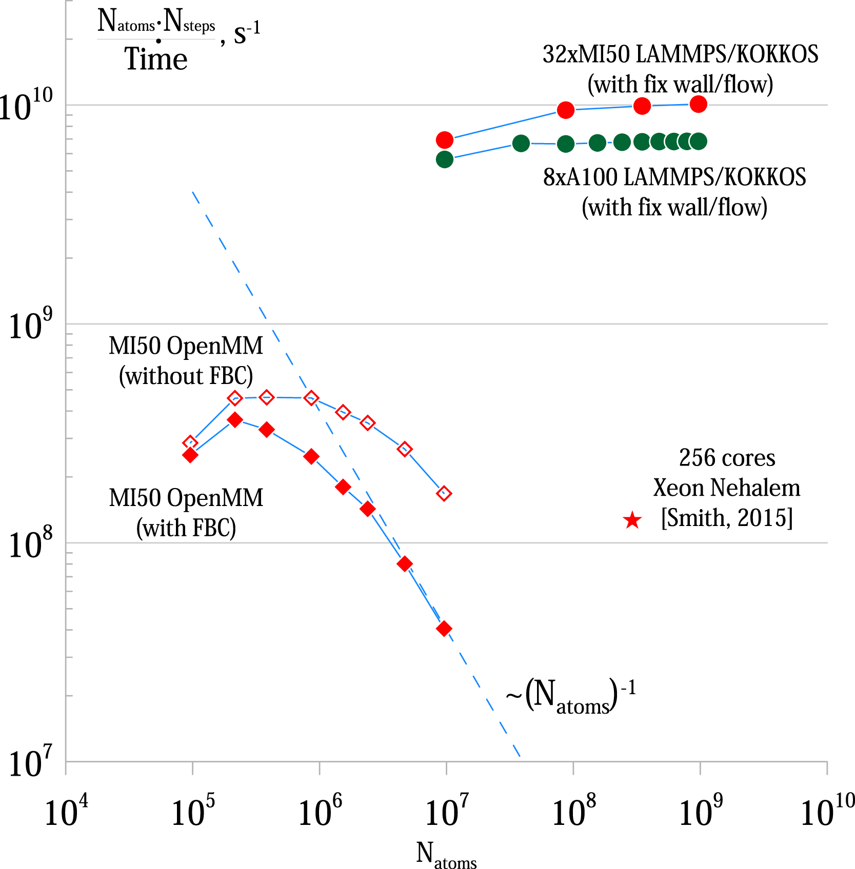

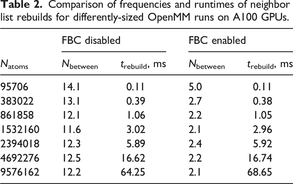
As will be discussed later, our hypothesis as to why our OpenMM implementation exhibits such a slowdown, was the increasing frequency of neighbor list rebuilds. To verify it, we have measured the frequency and average run time of the findBlocksWithInteractions kernel. This kernel is invoked on each step and it conditionally performs the expensive

O (N^{2})

neighbor list rebuild. We measured how often the condition is fulfilled and how long it takes for the kernel to run in that case. In particular, the two values of interest that we measured were N_between and t_rebuild in relation to N_atoms ⋅ N_between is the average amount of steps taken between neighbor list rebuilds. t_rebuild is the average run time of a single invocation. The measurements are presented in Table 2. The measurements suggest that while the cost of a single rebuild remains the same, the presence of FBC makes the rebuilding occur more often.

Table 2.

Comparison of frequencies and runtimes of neighbor list rebuilds for differently-sized OpenMM runs on A100 GPUs.

	FBC disabled		FBC enabled
N _atoms	N _between	t_rebuild, ms	N _between	t_rebuild, ms
95706	14.1	0.11	5.0	0.11
383022	13.1	0.39	2.7	0.38
861858	12.1	1.06	2.2	1.05
1532160	11.6	3.02	2.1	2.96
2394018	12.3	5.89	2.4	5.92
4692276	12.5	16.62	2.2	16.74
9576162	12.2	64.25	2.1	68.65

We also measured the strong scaling for a typical LAMMPS/Kokkos simulation with fix wall/flow. To gauge the severity of the bottleneck that appears when GPU-aware communication is unavailable (its development complexity has been described recently Khalilov et al. (2022)), we also added the measurements for when it is manually disabled. The results are demonstrated on Figure 2. There is a noticeable performance hit when transitioning from a single GPU to multiple GPUs in the absence of GPU-aware communication, other than that near-perfect scaling can be observed. The presence of the fix wall/flow only affects the overall performance by a constant factor 10%–20% but does not hamper the scaling.

Figure 2.

Strong scaling of wall/flow simulations using the LAMMPS/Kokkos package. Performance for 10000 steps with N_atoms = 60480000 (higher is better).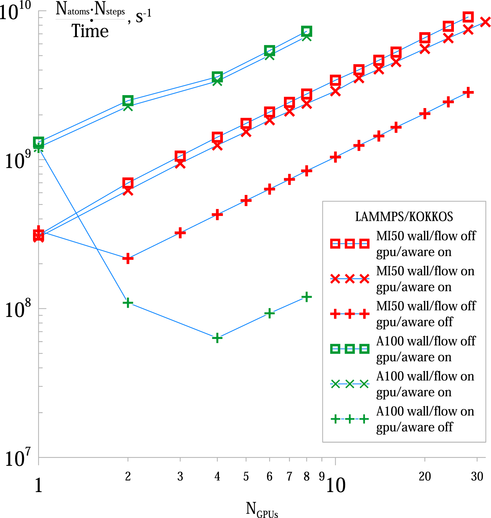

These benchmarks demonstrate that on bigger systems LAMMPS/Kokkos allows for excellent scaling for the entire range of our sample. We did not test the scaling of OpenMM because it does not implement domain decomposition and the only multi-GPU parallelization it can offer is offloading parts of the array of interacting tiles to other GPUs when computing forces. However, the most expensive part at these system sizes — the force matrix traversal — still happens on one GPU and is not parallelized.

We have performed a tracing analysis of LAMMPS/Kokkos on the Desmos supercomputer with Score-P ver. 8.1 (Knüpfer et al. (2012)) compiled with Kokkos and HIP profiling support. Tracing has been done with SCOREP_HIP_ENABLE=api parameter, which allows us to record all the HIP API calls. Short MD trajectories are considered for tracing with only 10 time steps and neighbor list rebuilding each 5 steps. To visualize trace data we use the Vampir tool (Knüpfer et al. (2008)). Figure 3 shows an example of the place of the fix wall/flow data exchange within the LAMMPS/Kokkos execution trace.

Figure 3.

Illustration of the 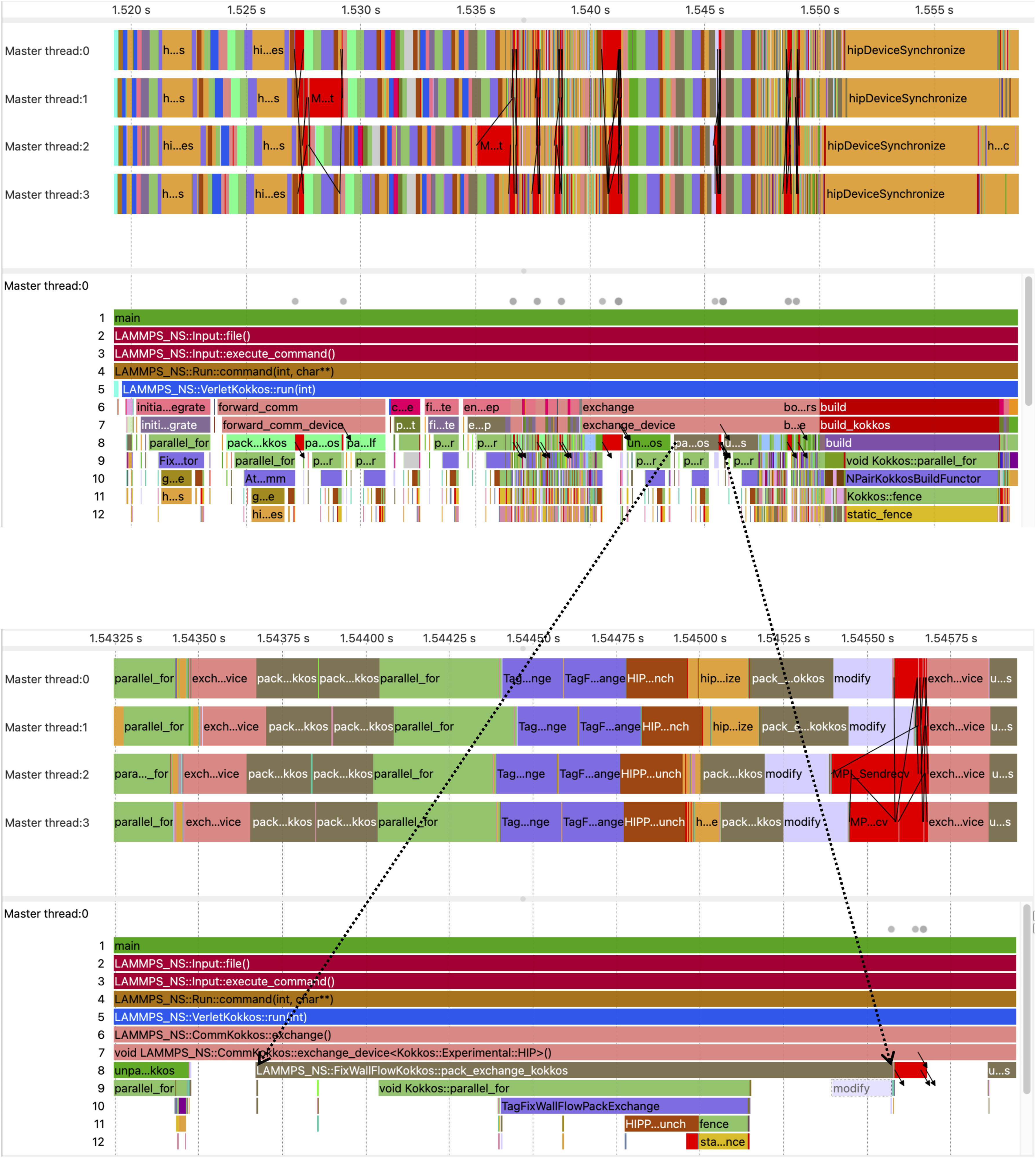fix wall/flow exchange in the LAMMPS/Kokkos run on 4 nodes, each with an MI50 GPU, of the Desmos supercomputer for a model with N_atoms = 604800. The master timeline and process timeline are visualized with the Vampir tool. The upper timeline shows 5 MD steps, the step with neighbor rebuilding included. The lower timeline shows the magnification for a fix wall/flow exchange.

Our trace analysis corroborates that the relative performance plunge with two or more GPUs compared to a single GPU happens due to the communication overhead, as can be seen on Figure 4. An acute difference can be seen in the amount of time spent inside the hipMemcpyAsync function that schedules the copying of data between the GPU and the host (the analysis of the traces on Figure 4 shows that MPI-calls in the non-GPU-aware case have slightly longer duration that can be expected since the bandwidth and the latency of GPU-GPU MPI-transfers are worse than for CPU-CPU MPI-transfers). Also, as can be seen on the Figure 2, without the ability to leverage the GPU-aware communication, simulations on A100 GPUs would run orders of magnitude slower.

Figure 4.

Juxtaposition of two traces: at the top is the trace of LAMMPS/Kokkos running with GPU-aware communication, at the bottom is the similar trace obtained without GPU-aware communication. The process timelines are shown on the left. Both runs were carried out on four Desmos supercomputer nodes with one MI50 GPU per node. For the sake of comparison of the traces, their alignment begins with the beginning of the 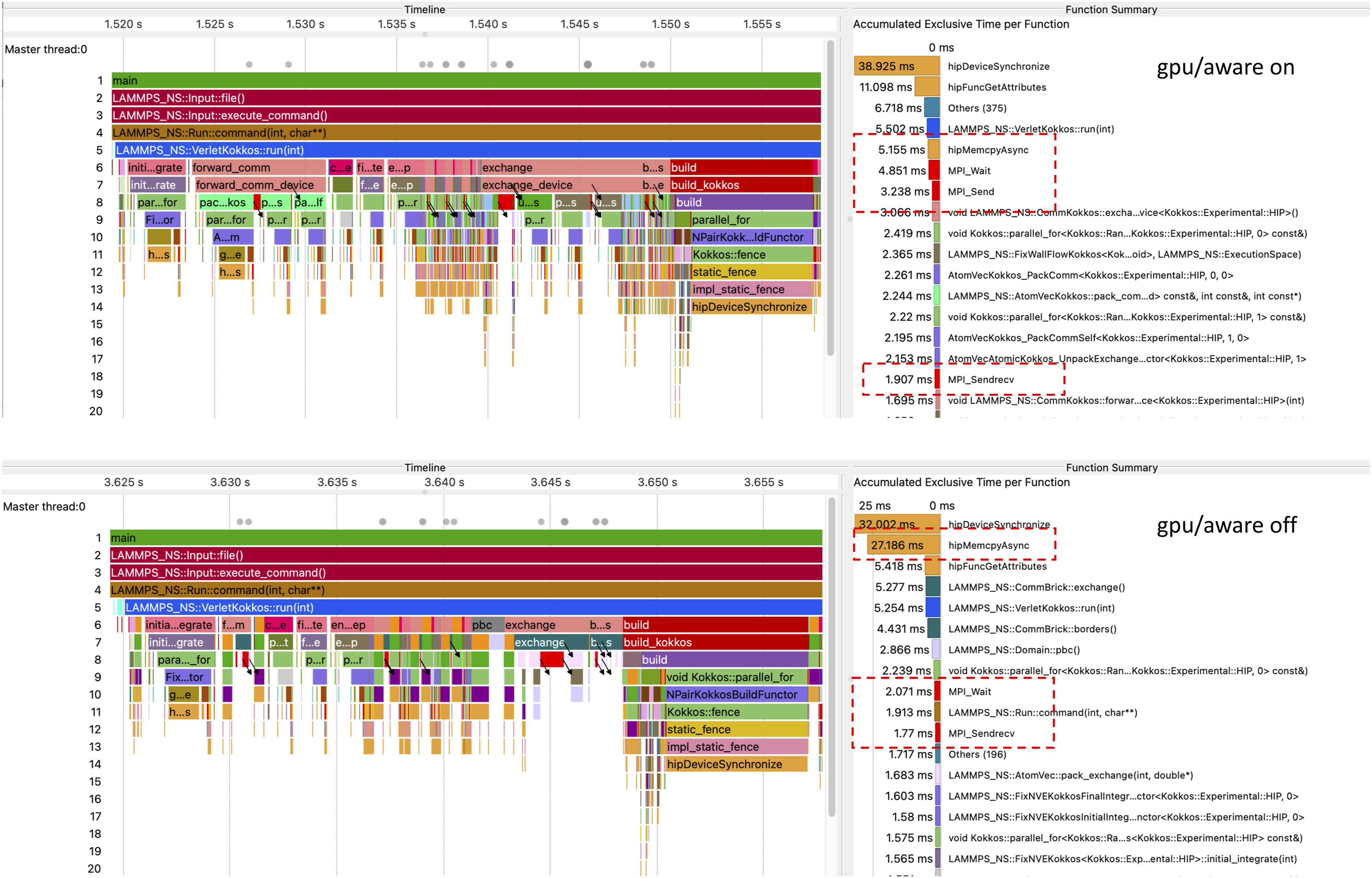LAMMPS_NS::VerletKokkos::run call and ends at the end of the build_kokkos call. The values of accumulated time per function are ranged on the right in the decending order.

6.2. Additional Flow Boundary Conditions planes

In our initial implementation, the only plane that was reassigning the particle velocities was the periodic boundary plane at the edges of the simulation box. This, however, proved insufficient due to the non-ideal nature of the fluid.

One undesirable effect cased by there being insufficient planes that can be observed is a “vorticity leakage”. An example of it can be seen on Figure 5. Adding extra FBC planes helps mitigating this issue and makes the flow more homogeneous.

Figure 5.

Side-by-side comparison of the vorticity plots of two identical systems with side ratio of 25:10:1 after some time has passed and stationary flow established. Here, N_atoms ≈ 3.25 × 10⁶ and v_flow = 3 with a cylindrical obstacle with r = 35. The left one has no extra FBC planes (one in total), the right one has five FBC planes. A much stronger vorticity leakage can be observed in the left system.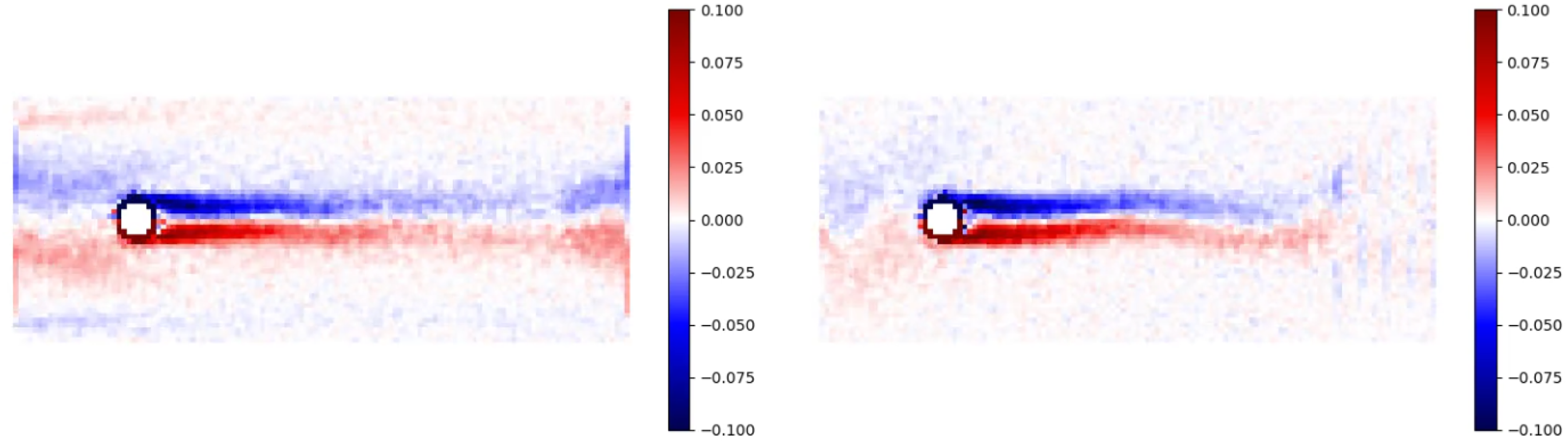

Another issue that can arise is that at higher flow velocities and higher system sizes particles can start accumulating near a downstream boundary. This particular effect is demonstrated on Figure 6.

Figure 6.

A system with N_atoms = 41 × 10⁶ and v_flow = 0.9. There are 4 additional FBC planes at the right side (five in total).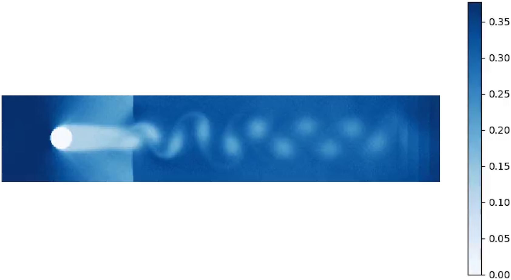

6.3. Calibration of flow velocity and tempterature

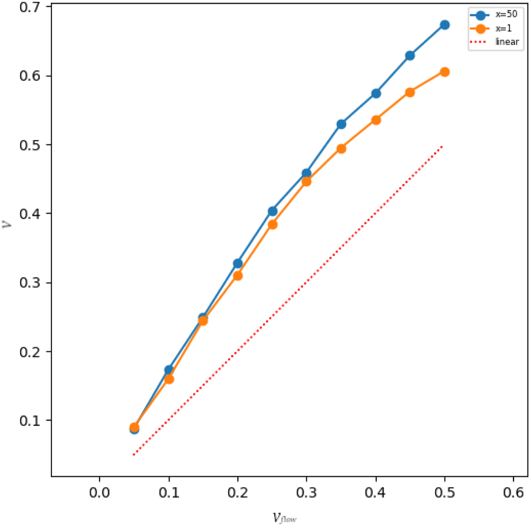
Since the premise upon which the distributions were derived was that the system consisted of ideal gas only, in more realistic scenarios this premise is certainly violated. This means that after putting a system into proposed FBC and letting the flow establishing after some time, the temperature and the actual flow velocity may not match the target ones. Figures 7 and 8 demonstrate how the achieved actual temperature and flow velocity differ from the target depending on the target flow velocity.

Figure 7.

Temperature over time for a system with N_atoms = 2.1 × 10⁶ for different target v_flow values. Target temperature is T₀ = 0.4 in all cases.

Figure 8.

Established velocity in the relative x = 1 and x = 50 positions (the left part and the middle part of the simulation box) depending on the target flow velocity in the system with N_atoms = 2.1 × 10⁶ for different target v_flow values. Target temperature is T₀ = 0.4 in all cases.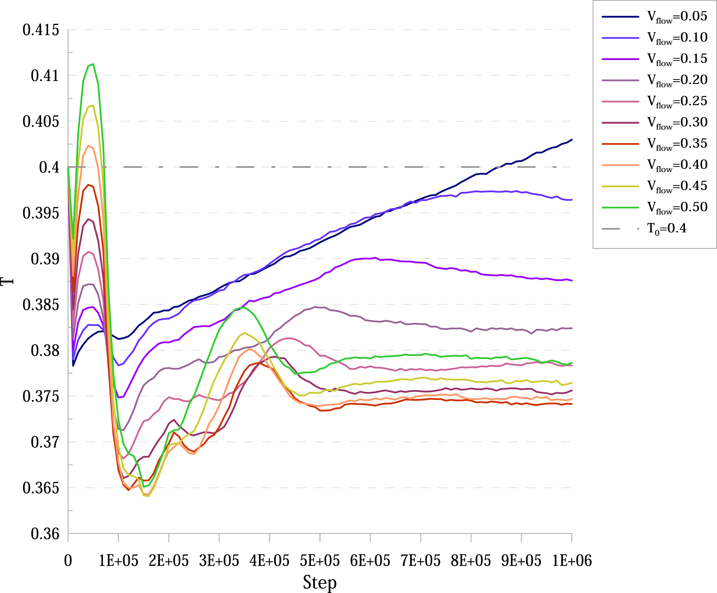

6.4. Pre-turbulent mode

As we are increasing the size of our simulation box, the nature of the flow is changing: at smaller scales it was laminar, at greater scales eddies began to appear as can be seen on Figure 9. We see that in the case of the Reynolds number Re ≈ 160 the Karman vortex street forms that is a typical feature of a pre-turbulent mode of the fluid flow.

Figure 9.

Density (left) and vorticity (right) plots for three different moments of time for a simulation with N_atoms = 41 × 10⁶ and v_flow = 0.5. Karman vortex street can be seen forming. The Reynolds number in this case is Re ≈ 160. There are 4 additional FBC planes at the right side (five in total).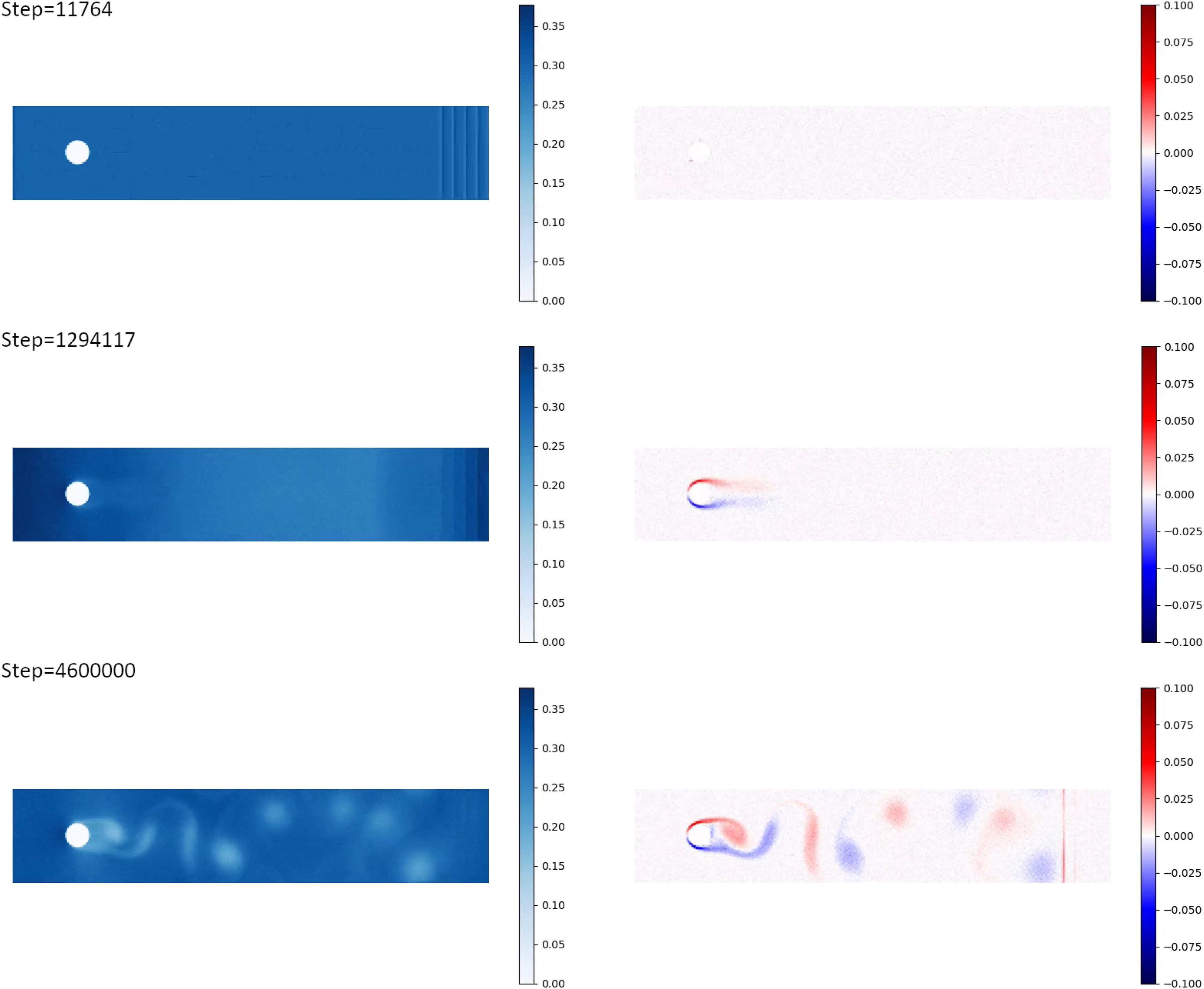

7. Discussion

Although the theoretical basis for our method is perfectly sound for ideal gases, as soon as we apply it to a non-ideal scenario, deviations from expected results such as vorticity leakages and density irregularities start to crop up. The likely cause of vorticity leakages is that particles on the opposite sides of a plane still interact with each other using short-range forces thereby “leaking” some information about vorticity on the other side.

The likely reason why density accumulates near the downstream boundary is that there is a higher-density region in front of the obstacle that repels particles that try to penetrate the boundary plane and many particles that do get through, get repelled right back into the plane, instantly losing all extra velocity. This results in a boundary being unable to “pump” the particles through in order to maintain a uniform and stationary flow. Luckily, this effect is apparent to the eye whenever it manifests, because a clear boundary between a lower-density and a higher-density region becomes visible on a density plot. Increasing the amount of planes or lowering the flow velocity helps alleviating this issue. For example, on Figure 9 the model dimensions are the same as on Figure 6 but there is no density transition because the flow velocity is lower.

One of the surprising performance effects that one of our implementations has is the progressive degradation of performance for the OpenMM implementation as the number of atoms increases. At first glance, it would seem that the neighbor list calculation that has $O (N^{2})$ complexity should drown out whatever linear performance costs introduced by the presence of the FBC. However, the nature of the slowdown suggests that the presence of the FBC indirectly causes the neighbor list recalculation to happen more often as demonstrated in Table 2, leaving room for future optimizations.

According to Smith (2015), it should be possible to observe turbulence at greater scales (at about N_atoms ≈ 3 × 10⁸, Re ≈ 400). Our LAMMPS/Kokkos implementation makes it possible to achieve these scales in the future if one were to dedicate sufficient GPU resources to such calculations. An interesting option for further development of the FBC method could be the adaptation for MD modelling of the turbulent inflow boundary conditions that are used in large eddy simulations Dhamankar et al. (2018). Our OpenMM implementation can be useful for studies of the vortex generation in non-Newtonian polymer fluids (e.g. see the recent papers of Handler et al. (2020) and Hopkins et al. (2020)) where the requirements for the number of atoms in MD models could be moderate but statistical averaging is important.

8. Conclusion

In this article, we have presented a novel type of flow boundary conditions for simulation of fluid flows on atomic level. We have described our GPU-based OpenMM implementation of this method, as well as the corresponding LAMMPS fix wall/flow implementaion and its Kokkos-accelerated variant. The special velocity distribution form that we use to reassign particle velocities makes it possible to correctly handle fluid flows with both high and low flow velocities due to the possibility to re-emit particles not only downstream but also upstream.

We have compared the performance of the OpenMM implementation with the LAMMPS/Kokkos implementation and analysed the strong scaling of the LAMMPS/Kokkos implementation on two multi-GPU systems, showing our implementation to be sufficiently scalable for running multi-billion MD models on multi-GPU supercomputers.

We have traced a typical LAMMPS/Kokkos MD run and shown the time taken by our fix wall/flow implementation as well as the importance of GPU-aware MPI communications for scalable MD calculations. We have demonstrated how to leverage the very new data transfer methods based on GPU-aware MPI in LAMMPS/Kokkos to speed up our custom fix wall/flow implementation.

Our LAMMPS/Kokkos fix wall/flow implementation opens up a possibility to conduct MD simulations of fluid flows at greater time and size scales than were accessible before by allowing scaling over multiple GPUs. In this work, we demonstrate the formation Karman vortex street in the model of 40 million atoms at Re ≈ 160 that corresponds to the pre-turbulent fluid flow mode. One can anticipate that by increasing the size of the MD model and the number of steps by 4-5, the Kolmogorov’s length scale can be resolved in such MD fluid flow models.

Footnotes

Acknowledgements

The authors are grateful to Yuri Grishichkin and Roman Chulkevich for the assistance with the system software tuning on the Desmos and cHARISMa supercomputers.

Declaration of conflicting interests

The author(s) declared no potential conflicts of interest with respect to the research, authorship, and/or publication of this article.

Funding

The development of the FBC algorithm and the performance analysis for the nodes of the Desmos supercomputer were supported by the Ministry of Science and Higher Education of the Russian Federation (agreement with the Joint Institute for High Temperatures of Russian Academy of Sciences). The implementation of the FBC algorithm in LAMMPS and the performance analysis for the nodes of the cHARISMa supercomputer were performed within the framework of the HSE University Basic Research Program.

ORCID iDs

Daniil Pavlov

Vladimir Stegailov

Author biographies

Daniil Pavlov is a master’s student at the Moscow Institute of Physics and Technology and an intern researcher at the Joint Institute for High Temperatures of Russian Academy of Sciences, Moscow, Russia. His research interests include high-performance computing and GPU computing in materials science, their scalability and portability.

Vladislav Galigerov is master’s student at the Higher School of Economics and an intern researcher at the Joint Institute for High Temperatures of Russian Academy of Sciences, Moscow, Russia. His research interests include high-performance computing, general-purpose GPU computing and atomistic simulations.

Daniil Kolotinskii is a junior researcher at the Laboratory of Supercomputer Methods in Condensed Matter Physics of Moscow Institute of Physics and Technology (MIPT) and a junior researcher at the Joint Institute for High Temperatures Russian Academy of Sciences. He obtained a master’s degree in Applied Mathematics and Physics from MIPT in 2021. Now he is a Ph.D student at MIPT. His research interests include computational physics, numerical modelling and parallel computing.

Vsevolod Nikolskiy is a research fellow at the International Laboratory for Supercomputer Atomistic Modelling and Multiscale Analysis of Higher School of Economics, Moscow, Russian, and a junior researcher at the Joint Institute for High Temperatures Russian Academy of Sciences. He obtained a master’s degree in Applied Mathematics and Informatics from the Moscow Institute of Electronics and Mathematics of the Higher School of Economics in 2018. Now he is a Ph.D. student of the Doctoral School of Computer Science of HSE University. His research interests include high-performance and heterogeneous computing, efficiency of novel processor architectures, development of GPU-accelerated algorithms.

Vladimir Stegailov graduated from the Moscow Institute of Physics and Technology in 2004, received a PhD degree in 2005 and a DrSc degree in 2012. He is Head of Department at the Joint Institute for High Temperatures of Russian Academy of Sciences, Moscow, Russia. He is a professor of the Higher School of Economics and a leading researcher in the International Laboratory for Supercomputer Atomistic Modelling and Multi-scale Analysis. He is a professor in the Moscow Institute of Physics and Technology where he leads the Laboratory of Supercomputer Methods in Condensed Matter Physics. His research interests include high-performance computing and atomistic and multiscale modelling and simulation.

References

Anderson

Lorenz

Travesset

(2008) General purpose molecular dynamics simulations fully implemented on graphics processing units. Journal of Computational Physics 227(10): 5342–5359. DOI: 10.1016/j.jcp.2008.01.047.

Antropov

Stegailov

(2023) Helium bubbles diffusion in aluminum: influence of gas pressure. Journal of Nuclear Materials 573: 154123. DOI: 10.1016/j.jnucmat.2022.154123.

Begau

Sutmann

(2015) Adaptive dynamic load-balancing with irregular domain decomposition for particle simulations. Computer Physics Communications 190: 51–61. DOI: 10.1016/j.cpc.2015.01.009.

Brown

Yamada

(2013) Implementing molecular dynamics on hybrid high performance computers—three-body potentials. Computer Physics Communications 184(12): 2785–2793. DOI: 10.1016/j.cpc.2013.08.002.

Brown

Wang

Plimpton

, et al. (2011) Implementing molecular dynamics on hybrid high performance computers — short range forces. Computer Physics Communications 182(4): 898–911. DOI: 10.1016/j.cpc.2010.12.021.

Brown

Kohlmeyer

Plimpton

, et al. (2012) Implementing molecular dynamics on hybrid high performance computers — particle-particle particle-mesh. Computer Physics Communications 183(3): 449–459. DOI: 10.1016/j.cpc.2011.10.012.

Chashechkin

Mitkin

(2001) Experimental study of a fine structure of 2D wakes and mixing past an obstacle in a continuously stratified fluid. Dynamics of Atmospheres and Oceans 34(2): 165–187. DOI: 10.1016/S0377-0265(01)00066-5.

Chorin

(1968) Numerical solution of the Navier-Stokes equations. Mathematics of Computation 22(104): 745–762. DOI: 10.2307/2004575.

de G Allen

Southwell

(1955) Relaxation methods applied to determine the motion, in two dimensions, of a viscous fluid past a fixed cylinder. Quarterly Journal of Mechanics & Applied Mathematics 8(2): 129–145. DOI: 10.1093/qjmam/8.2.129.

10.

Dhamankar

Blaisdell

Lyrintzis

(2018) Overview of turbulent inflow boundary conditions for large-eddy simulations. AIAA Journal 56(4): 1317–1334.

11.

Eastman

Pande

(2009) Efficient nonbonded interactions for molecular dynamics on a graphics processing unit. Journal of Computational Chemistry 31(6): 1268–1272. DOI: 10.1002/jcc.21413.

12.

Eastman

Friedrichs

Chodera

, et al. (2013) Openmm 4: a reusable, extensible, hardware independent library for high performance molecular simulation. Journal of Chemical Theory and Computation 9(1): 461–469. DOI: 10.1021/ct300857j.

13.

Eastman

Swails

Chodera

, et al. (2017) Openmm 7: rapid development of high performance algorithms for molecular dynamics. PLOS Comput. Biology 13: 1–17. DOI: 10.1371/journal.pcbi.1005659.

14.

Edwards

Trott

Sunderland

(2014) Kokkos: enabling manycore performance portability through polymorphic memory access patterns. Journal of Parallel and Distributed Computing 74: 3202–3216. DOI: 10.1016/j.jpdc.2014.07.003.

15.

Eijkhout

van de Geijn

Chow

(2016) Introduction to High Performance Scientific Computing. Geneva, Switzerland: Zenodo. DOI:10.5281/zenodo.49897.

16.

Fominykh

Nikolskiy

Stegailov

(2023) Atomistic model of an oxide film in contact with a liquid metal coolant: defects concentrations and chemical potentials of dissolved Fe–O. Computational Materials Science 220: 112061. DOI: 10.1016/j.commatsci.2023.112061.

17.

Galigerov

(2023) Fix Wall/flow Implementation. GitHub. Available at: https://github.com/vladgl/lammps/tree/fix_wall_flow

18.

Glaser

Nguyen

Anderson

, et al. (2015) Strong scaling of general-purpose molecular dynamics simulations on gpus. Computer Physics Communications 192: 97–107. DOI: 10.1016/j.cpc.2015.02.028.

19.

Grinberg

Insley

Morozov

, et al. (2011) A new computational paradigm in multiscale simulations: application to brain blood flow. Proceedings of 2011 International Conference for High Performance Computing, Networking, Storage and Analysis, Seattle, WA, 13–18 Nov. 2022, pp. 1–5. DOI: 10.1145/2063384.2063390.

20.

Hadjiconstantinou

(2006) The limits of Navier-Stokes theory and kinetic extensions for describing small-scale gaseous hydrodynamics. Physics of Fluids 18(11): 111301. DOI: 10.1063/1.2393436.

21.

Halver

Junghans

Sutmann

(2023) Using heterogeneous GPU nodes with a Cabana-based implementation of MPCD. Parallel Computing 117: 103033. DOI: 10.1016/j.parco.2023.103033.

22.

Handler

Blaisten-Barojas

Ligrani

, et al. (2020) Vortex generation in a finitely extensible nonlinear elastic peterlin fluid initially at rest. Engineering Reports 2(3): e12135. DOI: 10.1002/eng2.12135.

23.

Hitz

Heinen

Vrabec

, et al. (2020) Comparison of macro-and microscopic solutions of the riemann problem i. supercritical shock tube and expansion into vacuum. Journal of Computational Physics 402: 109077. DOI: 10.1016/j.jcp.2019.109077.

24.

Hitz

Jöns

Heinen

, et al. (2021) Comparison of macro-and microscopic solutions of the riemann problem ii. two-phase shock tube. Journal of Computational Physics 429: 110027. DOI: 10.1016/j.jcp.2020.110027.

25.

Hopkins

Gogovi

Weisel

, et al. (2020) Polyacrylamide in glycerol solutions from an atomistic perspective of the energetics, structure, and dynamics. AIP Advances 10(8): 085011. DOI: 10.1063/5.0020850.

26.

Kadau

Barber

Germann

, et al. (2010) Atomistic methods in fluid simulation. Philosophical Transactions of the Royal Society A: Mathematical, Physical & Engineering Sciences 368(1916): 1547–1560. DOI:10.1098/rsta.2009.0218.

27.

Kawaguti

(1953) Numerical solution of the Navier-Stokes equations for the flow around a circular cylinder at Reynolds number 40. Journal of the Physical Society of Japan 8(6): 747–757. DOI: 10.1143/JPSJ.8.747.

28.

Khalilov

Timofeev

Polyakov

(2022) Towards OpenUCX and GPUDirect technology support for the Angara interconnect. In: Russian Supercomputing Days. Berlin, Germany: Springer, pp. 591–603.

29.

Knüpfer

Brunst

Doleschal

, et al. (2008) The Vampir performance analysis tool-set. In: Resch

Keller

Himmler

, et al. (eds) .Tools for High Performance Computing. Berlin, Heidelberg: Springer Berlin Heidelberg, pp. 139–155.

30.

Knüpfer

Rössel

Mey

(2012) Score-P: a joint performance measurement run-time infrastructure for Periscope, Scalasca, TAU, and Vampir. In: Brunst

Müller

Nagel

, et al. (eds) Tools for High Performance Computing 2011. Berlin, Heidelberg: Springer Berlin Heidelberg, pp. 79–91

31.

Kolmogorov

(1941) Local structure of turbulence in an incompressible fluid at very high Reynolds numbers. Doklady Akademii Nauk SSSR 31: 99–101.

32.

Komatsu

Matsumoto

Shimada

Ito

(2014) A glimpse of fluid turbulence from the molecular scale. International Journal of Modern Physics C 25(8): 1450034. doi: 10.1142/S012918311450034X

33.

Kondratyuk

Nikolskiy

Pavlov

, et al. (2021) GPU-accelerated molecular dynamics: state-of-art software performance and porting from nvidia CUDA to AMD HIP. The International Journal of High Performance Computing Applications 35(4): 312–324. DOI: 10.1177/10943420211008288.

34.

Kondratyuk

Ryltsev

Ankudinov

, et al. (2023) First-principles calculations of the viscosity in multicomponent metallic melts: Al-cu-ni as a test case. Journal of Molecular Liquids 380: 121751. DOI: 10.1016/j.molliq.2023.121751.

35.

Kostenetskiy

Chulkevich

Kozyrev

(2021) HPC resources of the higher School of Economics. Journal of Physics: Conference Series 1740(1): 012050. DOI: 10.1088/1742-6596/1740/1/012050.

36.

Kutzner

Páll

Fechner

, et al. (2015) Best bang for your buck: GPU nodes for GROMACS biomolecular simulations. Journal of Computational Chemistry 36(26): 1990–2008. DOI: 10.1002/jcc.24030.

37.

Kutzner

Páll

Fechner

, et al. (2019) More bang for your buck: improved use of GPU nodes for GROMACS 2018. Journal of Computational Chemistry 40(27): 2418–2431. DOI: 10.1002/jcc.26011.

38.

Lykov

Lei

, et al. (2015) Inflow/outflow boundary conditions for particle-based blood flow simulations: application to arterial bifurcations and trees. PLoS Computational Biology 11(8): e1004410.

39.

Nguyen-Cong

Willman

Moore

, et al. (2021) Billion atom molecular dynamics simulations of carbon at extreme conditions and experimental time and length scales. In: Proceedings of the International Conference for High Performance Computing, Networking, Storage and Analysis. New York, NY: Association for Computing Machinery. DOI: 10.1145/3458817.3487400.

40.

Nikolskiy

Stegailov

(2020) GPU acceleration of four-site water models in LAMMPS. Parallel Computing: Technology Trends. Amsterdam, Netherlands: IOS Press, pp. 565–573.

41.

Pavlov

(2022b) Patch for tileIndex Variable Size in OpenMM. GitHub. https://github.com/openmm/openmm/pull/3577.

42.

OpenMM team (2023b) OpenMM Library Level C++/Python API. http://docs.openmm.org/development/api-c++/

43.

OpenMM team (2023a) Openmm Application Layer python API. http://docs.openmm.org/latest/api-python/app.html

44.

Pavlov

(2022a) OBC Implementation in OpenMM. GitHub. https://github.com/dann239/openmm/tree/open-boundary

45.

Pavlov

Kolotinskii

Stegailov

(2023) GPU-based molecular dynamics of turbulent liquid flows with OpenMM. In: Wyrzykowski

Dongarra

Deelman

, et al. (eds) Parallel Processing and Applied Mathematics. Cham: Springer International Publishing, pp. 346–358

46.

Plimpton

(1995) Fast parallel algorithms for short-range molecular dynamics. Journal of Computational Physics 117(1): 1–19. DOI: 10.1006/jcph.1995.1039.

47.

Priezjev

(2007) Rate-dependent slip boundary conditions for simple fluids. Physical Review E 75(5): 051605.

48.

Priezjev

(2013) Molecular dynamics simulations of oscillatory Couette flows with slip boundary conditions. Microfluidics and Nanofluidics 14: 225–233.

49.

Rapaport

Clementi

(1986) Eddy formation in obstructed fluid flow: a molecular-dynamics study. Physical Review Letters 57: 695–698. DOI: 10.1103/PhysRevLett.57.695.

50.

Sergeenko

Svirid

Afremov

, et al. (2022) Demonstration of the model of physicochemical processes in heavy liquid metal cooled reactors in an example of the THEADES experiment simulation. Nuclear Engineering and Design 395: 111870. DOI: 10.1016/j.nucengdes.2022.111870.

51.

Shamsutdinov

Khalilov

Ismagilov

, et al. (2021) Performance of supercomputers based on angara interconnect and novel amd cpus/gpus. In: Balandin

Barkalov

Gergel

, et al. (eds) Mathematical Modeling and Supercomputer Technologies. Cham: Springer International Publishing, pp. 401–416. DOI: 10.1007/978-3-030-78759-2_33.

52.

Shaw

Adams

Azaria

, et al. (2021) Anton 3: twenty microseconds of molecular dynamics simulation before lunch. In: Proceedings of the International Conference for High Performance Computing, Networking, Storage and Analysis. New York, NY: Association for Computing Machinery, pp. 1–11.

53.

Simuni

(1964) Numerical solution of some problems of flow of viscous liquids (in Russian). Inshenernyj Shurnal 4: 446–450.

54.

Smith

(2015) A molecular dynamics simulation of the turbulent Couette minimal flow unit. Physics of Fluids 27(11): 115105. DOI: 10.1063/1.4935213.

55.

Smith

Trevelyan

Ramos-Fernandez

, et al. (2020) CPL library — a minimal framework for coupled particle and continuum simulation. Computer Physics Communications 250: 107068. DOI: 10.1016/j.cpc.2019.107068.

56.

Stegailov

Dlinnova

Ismagilov

, et al. (2019) Angara interconnect makes GPU-based Desmos supercomputer an efficient tool for molecular dynamics calculations. The International Journal of High Performance Computing Applications 33(3): 507–521. DOI: 10.1177/1094342019826667.

57.

StreamHPC (2023) OpenMM HIP Plugin. GitHub. Available at: https://github.com/StreamHPC/openmm-hip

58.

Taniguchi

(2019) Kokkos Exchange Comm for Fixes 1394. GitHub. Available at: https://github.com/lammps/lammps/pull/1394

59.

Tchipev

Seckler

Heinen

, et al. (2019) Twetris: twenty trillion-atom simulation. Int. J. High Perf. Comp. Applications 33(5): 838–854. DOI: 10.1177/1094342018819741.

60.

Thompson

Aktulga

Berger

, et al. (2022) LAMMPS - a flexible simulation tool for particle-based materials modeling at the atomic, meso, and continuum scales. Computer Physics Communications 271: 108171. DOI: 10.1016/j.cpc.2021.108171.

GPU-based molecular dynamics of fluid flows: Reaching for turbulence

Abstract

Keywords

1. Introduction

2. Related work

3. Software

3.1. OpenMM

3.2. LAMMPS

4. Flow Boundary Conditions

4.1. Derivation of Flow Boundary Conditions for an ideal gas

4.2. Flow Boundary Conditions algorithm

4.3. OpenMM implementation

4.4. LAMMPS implementation

4.5.1. Kokkos-accelerated version

5. Grid aggregation

5.1. Distributed grids aggregation in LAMMPS

6. Simulation results

6.1. Performance comparison

6.2. Additional Flow Boundary Conditions planes

6.3. Calibration of flow velocity and tempterature

6.4. Pre-turbulent mode

7. Discussion

8. Conclusion

Footnotes

Acknowledgements

Declaration of conflicting interests

Funding

ORCID iDs

Author biographies

References