On the path to exascale the landscape of computer device architectures and corresponding programming models has become much more diverse. While various low-level performance portable programming models are available, support at the application level lacks behind. To address this issue, we present the performance portable block-structured adaptive mesh refinement (AMR) framework Parthenon, derived from the well-tested and widely used Athena++ astrophysical magnetohydrodynamics code, but generalized to serve as the foundation for a variety of downstream multi-physics codes. Parthenon adopts the Kokkos programming model, and provides various levels of abstractions from multidimensional variables, to packages defining and separating components, to launching of parallel compute kernels. Parthenon allocates all data in device memory to reduce data movement, supports the logical packing of variables and mesh blocks to reduce kernel launch overhead, and employs one-sided, asynchronous MPI calls to reduce communication overhead in multi-node simulations. Using a hydrodynamics miniapp, we demonstrate weak and strong scaling on various architectures including AMD and NVIDIA GPUs, Intel and AMD x86 CPUs, IBM Power9 CPUs, as well as Fujitsu A64FX CPUs. At the largest scale on Frontier (the first TOP500 exascale machine), the miniapp reaches a total of 1.7 × 10¹³ zone-cycles/s on 9216 nodes (73,728 logical GPUs) at weak scaling parallel efficiency (starting from a single node). In combination with being an open, collaborative project, this makes Parthenon an ideal framework to target exascale simulations in which the downstream developers can focus on their specific application rather than on the complexity of handling massively-parallel, device-accelerated AMR.
From a computational point of view, simulating these problems involves solving (various types of) partial differential equation—often on a structured grid using finite volume or finite difference methods. However, given the physical scale separation these problems typically cannot be globally represented in simulations—even on the next generation, exascale supercomputers. One option to make these kinds of simulations feasible is the use of (adaptive) mesh refinement (AMR), that is, a mesh that increases the spatial resolution in regions of interest. AMR frameworks using varying refinement approaches have successfully been used for many years. These include refinement based on individual cells, for example in RAMSES (Teyssier, 2002) or xRAGE (Gittings et al., 2008), based on separate patches (of arbitrary shape and size), for example, by Berger and Colella (1989) implemented in Enzo (Brummel-Smith et al., 2019) and Pluto (Mignone et al., 2011), or based on blocks of fixed size, for example, as in PARAMESH (MacNeice et al., 2000). With respect to parallelization all these “legacy” frameworks are primarily concerned with handling the mesh (and its refinement) across multiple nodes in parallel, see, for example, Dubey et al. (2014) for a comparative review. Given that they were developed prior to the broad availability of accelerators/GPUs, the additional levels of parallelism and memory hierarchy provided by these devices are typically not leveraged. This prevents an efficient use of those frameworks on many next generation, exascale supercomputers.
From a technical point of view, achieving sustained application-level exascale performance will require maximizing concurrency throughout the application while simultaneously minimizing the impact of data movement within the system. Both issues will be significantly more challenging at exascale than they are on today’s petascale systems: Amdahl’s law will require ever more levels of parallelism to be exploited in applications to remove or hide even small sequential bottlenecks. At the same time, technological trends will continue to increase the expense of data movement relative to compute for most applications as well as introduce more dynamic performance characteristics due to power capping and highly tapered network topologies. An additional challenge is that applications will need to achieve this level of performance on two or more radically different system architectures, as typified by the current Summit (IBM/Nvidia) and Frontier (AMD), and future El Capitan (AMD) and Aurora (Intel) systems. These requirements are pushing applications to consider new programming approaches such as additional hardware abstraction layers, and/or compositions of task-based and data parallelism.
In general, the combination of accelerated nodes (with large amounts of device memory and different architectures) and the complexity of AMR introduces new compuational challenges. For example, handling many (even up to thousand of) blocks per device with even more compute kernels—especially when small block sizes are involved—can result in significant overheads both with respect to managing the mesh hierarchy as well as with respect to the cumulated kernel launch latency.
To address these challenges, we introduce the performance portable block-structured adaptive mesh refinement framework Parthenon. It is built on the basis of Athena++ (Stone et al., 2020) and K-Athena (Grete et al., 2021a) and hides the complexity of AMR and device computing in downstream codes by providing high-level abstractions. These high-level abstractions not only pertain to the handling of the mesh and its data but also address computational complexity, such as parallel execution. To exploit on-node data parallelism, Parthenon internally uses the performance portability programming model Kokkos (Carter Edwards et al., 2014; Trott et al., 2021). This way Parthenon inherits the Kokkos capability to target various device architectures using a single source code and programming model. To further increase data parallelism, Parthenon also supports various levels of logical packing of data structures such as variables or even entire blocks, which are always allocated in device memory to minimize data transfer. To exploit inter-node parallelism, Parthenon internally uses asynchronous, one-sided (GPU-aware) MPI calls using buffers located in device memory.
Naturally, the Parthenon collaboration is not the only collaboration who has identified the various numerical and computational issues of “next generation” AMR frameworks. For example, AMReX (Zhang et al., 2021) shares many design decisions with Parthenon including data containers and abstraction for parallel regions. Key differences to Parthenon are the more flexible mesh structure in AMReX (at the cost of increased complexity) and a self-contained performance portability layer rather than relying on an external library such as Kokkos. Another example is Uintah (Holmen et al., 2017), which, as a legacy asynchronous many-task runtime system for block-structured AMR, also adopted Kokkos internally as performance portability layer below an intermediate abstraction layer. While Parthenon also offers a flexible, asynchronous tasking system, it is operating at the block level whereas Uintah tasks can be more fine-grained following a directed acyclic graph. However, to our knowledge the impact performance of the interplay of fine-grained tasks with (many) kernel launches and large number of blocks per device is still an open question. This similarly applies to other asynchronous many-task runtime systems such as Charm++ who also start to incorporate GPU support (Choi et al., 2022). One framework using AMR built on top of Charm++ is Quinoa (Bakosi et al., 2021) that just started to use GPUs. Finally, gamer-2 is astrophysical, multi-physics code with support for GPU-accelerated AMR (Zhang et al., 2018). It differs from Parthenon by being a fully integrated code (physics and mesh) rather than an AMR framework and supporting only CUDA (i.e., Nvidia GPUs). Moreover, in gamer-2 all data structures are allocated in host memory so that data required in compute kernels is constantly transferred back and forth between host and device memory.
In the following, we first provide a brief background on block-structured AMR and Kokkos in Section 2 before introducing the key design aspects and features of Parthenon in Section 3. In Section 4, we provide an overview of various downstream applications that are built on top of Parthenon including the Parthenon-hydro miniapp. The latter is used in Section 5 to present different performance characteristics of Parthenon pertaining to the packing of variables and blocks as well as to weak and strong scaling. In Section 6, we describe the software engineering approach taken by the collaboration. Finally, we discuss current limitations and future enhancements in Section 7 before we conclude in Section 8.
2. Background
2.1. Block-structured AMR
Only a brief summary of the block-structured AMR algorithm adopted by Parthenon is given in what follows, a complete description is given in Stone et al. (2020). Individual cells that span the computational domain are grouped into a regular array of subvolumes termed MeshBlocks. Data associated with the cells on a given MeshBlock are stored as N-dimensional arrays. Parthenon provides infrastructure for AMR with both cell- and face-centered data. The size of these arrays must be the same on all MeshBlocks, and moreover the overall domain must contain an integer number of MeshBlocks in each dimension. However, the number and size of individual MeshBlocks tiling the computational domain is arbitrary.
The MeshBlocks themselves are arranged into a binary-tree (in 1D), a quad-tree (in 2D), or an oct-tree (in 3D). Use of a tree greatly simplifies finding neighbors (necessary for communicating boundary conditions) and allows distribution of MeshBlocks across multiple processers using Z-ordering, which helps improve load balancing.
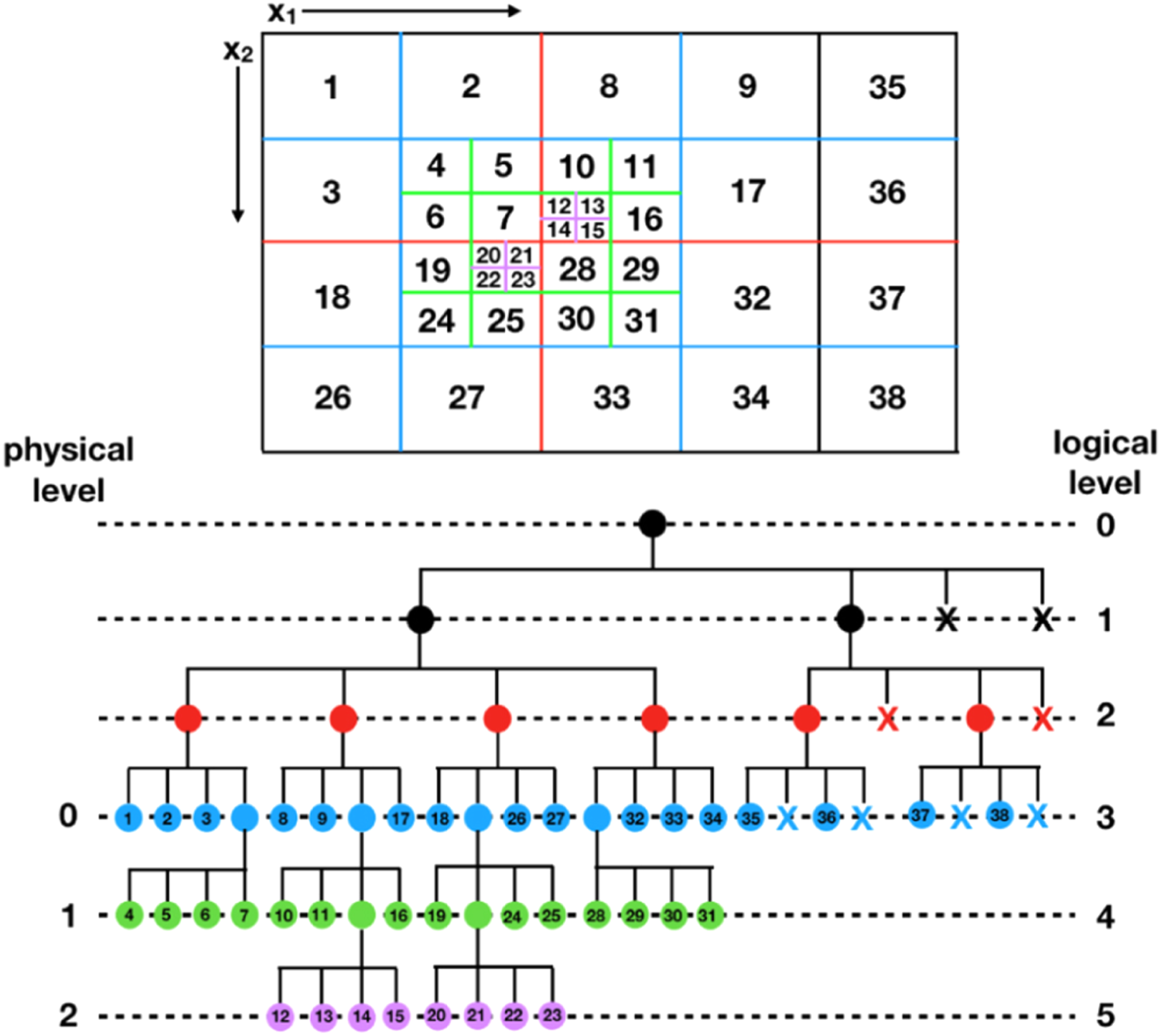
For AMR calculations, any number of MeshBlocks can be subdivided into 2N finer MeshBlocks (prolongation), or contiguous blocks of 2NMeshBlocks can be joined into one coarser MeshBlock (restriction), as needed. Figure 1 diagrams how MeshBlocks on a refined grid are stored in the tree. The tree structure ensures that the neighbors of a MeshBlock can easily be found, even if they are at different levels of the grid hierarchy. One great advantage of this tree structure-based AMR is that any given spatial location in the domain is covered by one, and only one, MeshBlock. As a result, only neighbor relationships exist but no spatial parent–child ones. Thus, except when new MeshBlocks are created or destroyed, prolongation and restriction is required only when data is communicated at MeshBlock boundaries. However, this approach requires that the entire tree is rebuilt every time (de)refinement is triggered and MeshBlocks are being destroyed/constructed in place.
Labeling of MeshBlocks (top) and their organization into a quadtree (bottom) for an example simulation with mesh refinement in two dimensions. Reproduced by permission of the AAS from Stone et al. (2020).
2.2. Kokkos
Kokkos is an open source, performance portable programming model for many core devices implemented as a C++ template based library (Carter Edwards et al., 2014; Trott et al., 2021). As such it provides abstractions to leverage hardware features, for example, threading or multi-level memory hierarchies, through various backends. This allows device-specific optimization at compile time for devices from various vendors, for example, using the CUDA backend for NVIDIA GPUs, the HIP backend for AMD GPUs, or the OpenMP backend for multi-threading on CPUs.
Some of the fundamental abstractions provided by Kokkos include:
• Execution Spaces define where (on which device/through which backend) a computational kernel (in practice a function object) is executed.
• Execution Patterns define how individual work items within a kernel are related. Examples include Kokkos::parallel_for for independent work items that can be handled independently in parallel or Kokkos::parallel_reduce to execute a parallel reduction over all work items.
• Execution Policies allow control over how a parallel region is executed. They can be simple, such as a RangePolicy that correspond to a single one-dimensional index for each work item, as well as nested loops, or they can be complex descriptions through hierarchical parallelism to control the grouping of threads and individual threads.
• Memory Spaces define where data is stored, for example, on the host or in device memory, or even in cache-type memory (where supported by hardware).
• Memory Layout allows to specify how data is stored, that is, how multidimensional indices are mapped to memory locations.
• Views are the primary data structure provided by Kokkos. They correspond to multidimensional arrays and are parameterized, for example, by a Memory Spaces and a Memory Layout.
3. Design
3.1. Primary design goals
Many algorithms employed in targeted application domains have comparatively low arithmetic intensity, for example, floating point operations per byte of data moved for stencil based calculation. At the same time, the peak compute power of devices has been increasing faster than the peak memory bandwidth in recent years and is even worse for the bandwidth between host memory and device (e.g., GPU) memory. This results in an ever increasing bottleneck when lots of data needs to be moved. To circumvent this, Parthenon follows a device first or device resident approach in which all work data is allocated in device memory only. In other words, data movement between host and devices is reduced to a minimum as the work data used in (expensive) computational kernels is already close to the execution space.
Another goal is to hide complexity from a downstream application point of view. Similar to Kokkos, which abstracts the complexity of on-node parallel programming, Parthenon generally provides additional abstractions to hide the complexity of multi node, parallel, block-structured adaptive mesh refinement. This includes simplified loop abstractions (i.e., setting many default values in the Kokkos layer) as well as higher level abstractions such as control over the packing of individual blocks, communication between nodes via MPI, a tasking infrastructure, or IO, as detailed in the following sections. At the simplest level, a downstream application only needs to provide compute kernels in plain C++ (i.e., no vendor specific backend) that are concerned with data of a single block and everything else is handled by Parthenon.
Importantly, the underlying access patterns provided by these abstractions need to change depending on hardware and must often be tuned for a given problem. To accomodate this constraint, we expose in our abstraction layers tuning parameters, allowing us to tune to individual hardware configurations.
Finally, Parthenon is designed with extensibility in mind offering many “plug-and-play” interfaces. This allows for a straightforward addition of many capabilities in downstream codes without requiring changes in Parthenon itself. At the same time, this also allows different downstream applications to easily share code as all downstream features are implemented using those interfaces by construction.
3.2. Intermediate abstraction layer
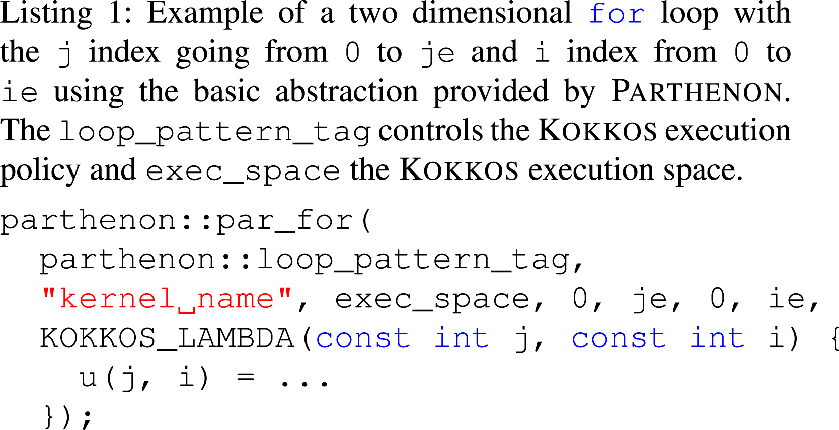
A given set of hardware may require different loop patterns and nested parallelism for optimal performance. For example, an Intel machine parallelized only with MPI may be most performant with a standard C++ for loop, enabled with vectorization pramgas. However, this will obviously not be the case on a GPU. Following the work in Grete et al. (2021a), we introduce a set of loop abstractions, which we call parthenon::par_for and parthenon::par_reduce. At their simplest, these are thin wrappers around Kokkos parallel dispatch. However, they have a unified interface suited to parthenon loops over meshblocks, regardless of the parallelism pattern used “under the hood.” This enables us to swap out Kokkos loops for basic for loops and calls to the C++ standard library. An example two-dimensional using the basic abstraction might look like
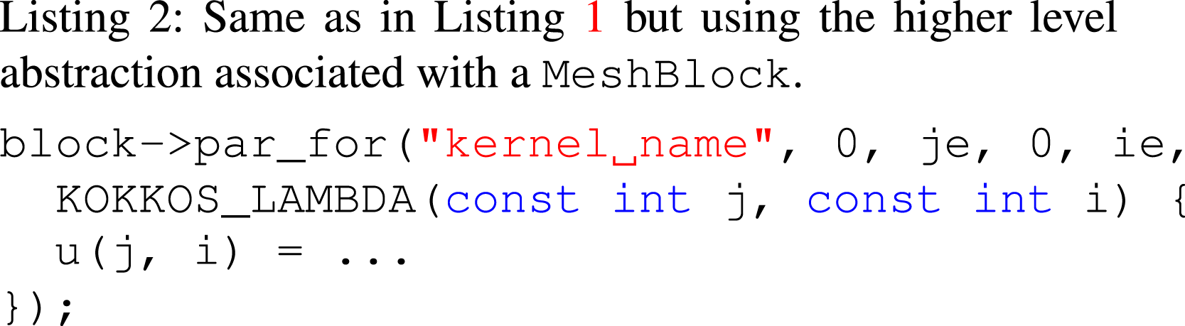
For ease of use, Parthenon sets several default options, such as the parallel pattern, at compile time depending on the target architecture. These are used when the par_for associated with a MeshBlock are used as illustrated in the following listing.
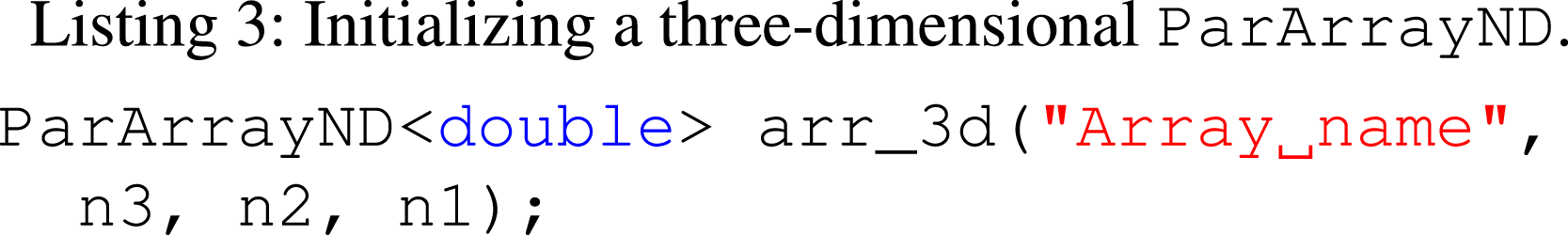
We also introduce an arbitrary rank array abstraction, built on Kokkos::View, which we call ParArrayND. To support Kokkos layout machinery, we use a six-dimensional Kokkos::View as the underlying data structure, and provide a suite of methods for accessing the elements of the array, casting it into a Kokkos::View, and getting lower-dimensional slices. This allows us to treat scalar, vector, and tensor variables all in the same way. For example, a three-dimensional array can be allocated as shown in Listing 3.
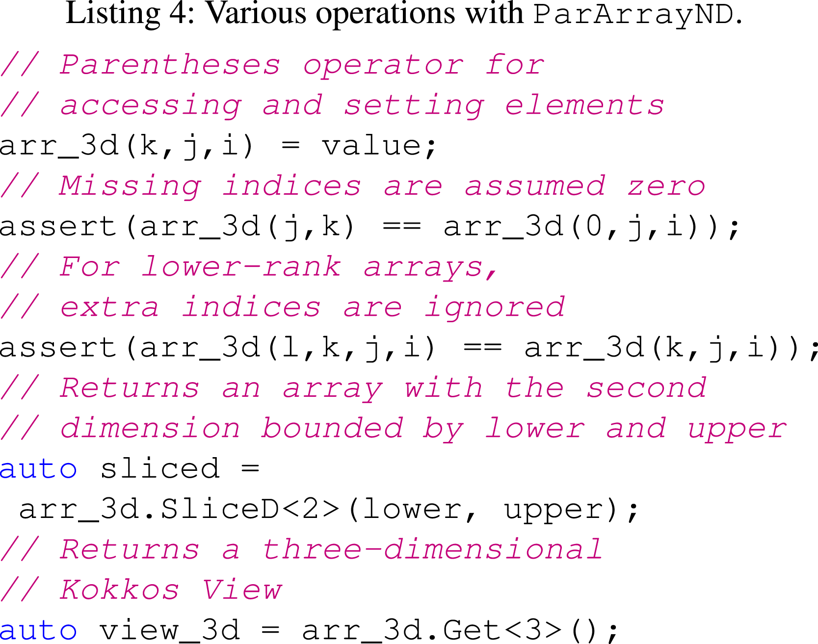
The shape is set by n3, through n1. Our convention is that the slowest-moving index is first in the constructor arguments and higher rank. However, this depends on the underlying Kokkos memory layout setting. (We currently assume LayoutLeft.) Our ParArrayND abstraction supports access operators, where missing indexes are assumed zero, slice operators, and access to the underlying Kokkos::View, as shown in Listing 4.
Both host and device ParArrayND objects are supported, but they default to living in device memory.
3.3. Packages
Parthenon is designed to couple multiple disparate components together. To capture this, we introduce packages. Each package is an independent functionality built on top of Parthenon, with its own registered variables, physics routines, and tasks. Importantly, packages can share variables. In other words, package “A” may register a variable and package “B” may use it. Parthenon supports dependency tracking between variables registered by packages. A package may register a variable as
• Private
• Provides
• Requires
• Overridable
A Private variable is private to a given package, and lives in the package’s namespace. Other packages should not access it. A Provides variable is provided by a package, with the intent that other packages may use it. However, the providing package is expected “own” the variable. If two packages try to provide the same variable, an error is raised. If a package registers a Requires variable, it is stating that it needs this variable to exist, but does not create or manage it itself. If no package provides a required variable, an error is raised. If a package registers an Overridable variable, it is stating that it can provide this variable, but will defer to another package, if it provides it.
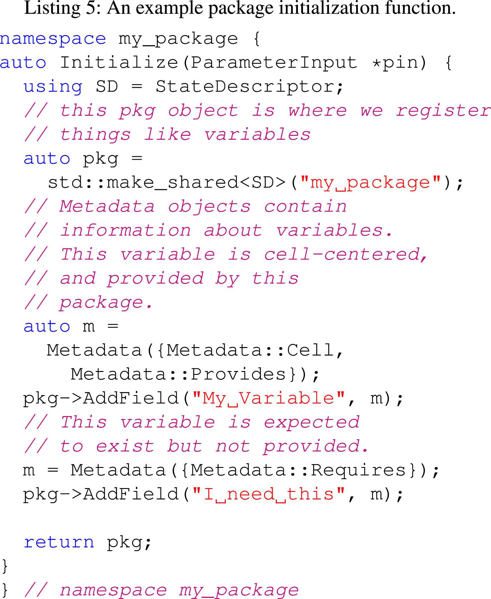
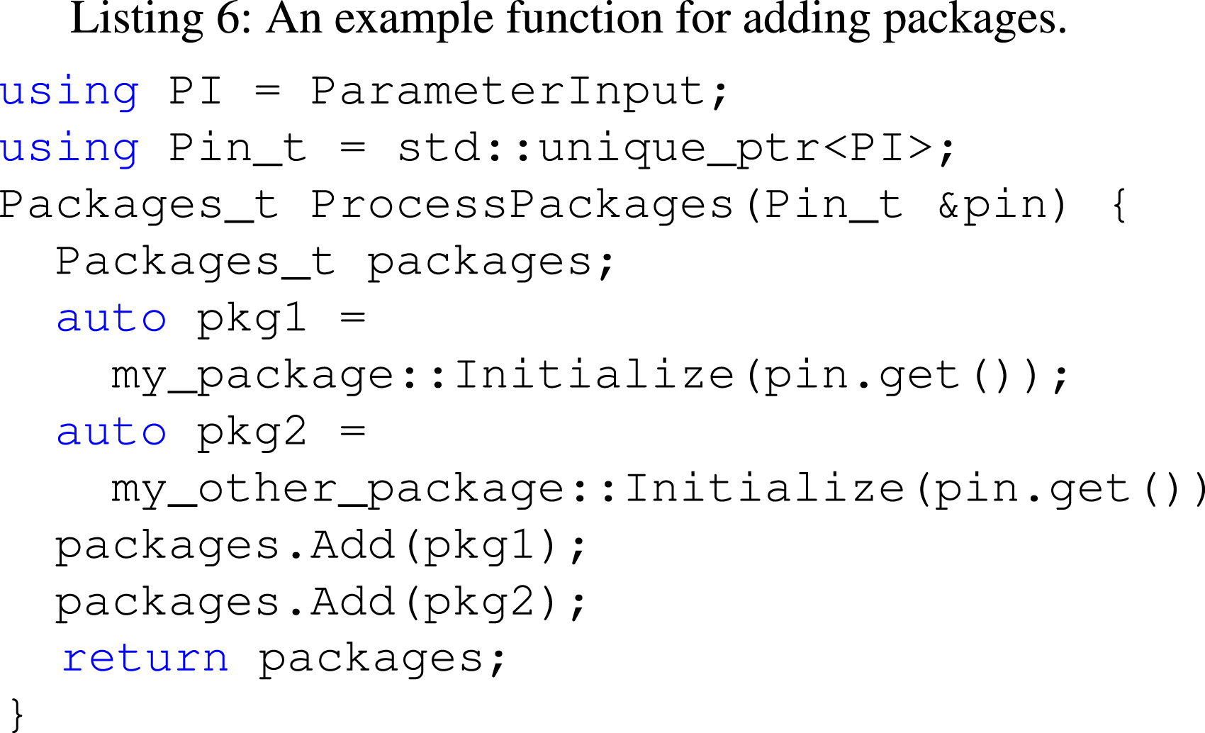
Packages register their variables, as well as global constants within their namespace (called params) in a function we call Initialize. An example Initialize function is shown in Listing 5. All initializations are registered by the parthenon manager object at startup. To tell the code what packages to load, a ProcessPackages function must be provided. An example function is shown in Listing 6.
Note that although packages create their own variables and provide tasks, these tasks are not automatically called. The tasks must be woven together “by hand” by an expert in the driver code. This will be explained in Section 3.10.
3.4. Variables
Variables in Parthenon consist of metadata and data. The data is stored on a per-block basis in a multidimensional Kokkos::View. It can live at cell centers, faces, edges, corners, or not be associated with a mesh entity at all. Although in the initial Parthenon release, only cell-centered and non-mesh-tied variables are fully implemented. Support for the other types of variables will be added in a later release.
All variables in Parthenon must be named. The name is used in simulation output, error messages, and to obtain a handle to the variable data from containers (see Section 3.6 ). This greatly enhances the readability and self-documentation of the code. The name of a variable is stored in its metadata along with other important information. The metadata also contains the shape of the variable, that is, if it is a scalar, vector, or tensor, along with the number of components in each dimension in the case of vectors and tensors. Finally, the metadata contains a collection of flags that indicate, for example, if the variable is independent or derived, whether it is private, provided, required, or overridable (see previous section), if it is advected, if it needs ghost cells filled, or if it has fluxes.
The metadata information allows the Parthenon infrastructure to perform certain tasks on variables without needing to understand their physical meaning. For example, Parthenon can write a restart file that includes only the independent variables, since they are all flagged as such. When using reflective boundary conditions, Parthenon can reflect the X-component of vector variables in the X-direction, Y-components in the Y-direction, and so on. Furthermore, the metadata flags are also useful for user provided physics packages. For example, the hydro package can advect all variables from all packages flagged as advected, without needing to know what those variables are. By setting the FillGhost and WithFluxes metadata flags, the user can control which variables will have their ghost cells filled by Parthenon and which variables will have fluxes buffers allocated.
Typically, variables are allocated on every block in the entire domain. But for some applications, there may be variables that are only relevant in parts of the domain, thus creating opportunities to save both memory and computing resources. For such cases, Parthenon provides sparse variables. Sparse variables behave just like ordinary (or dense) variables, with two exceptions: (i) Instead of just a name, sparse variables have a base name and a sparse ID and (ii) sparse variables are only allocated on some blocks.
Sparse variables are added through pools. A sparse pool consists of a base name, a set of sparse IDs, and shared metadata. For each sparse ID in the pool (e.g., 1, 4, 10, and 11), a sparse variable is created whose name is “basename_X”, where “basename” is the pool’s basename and “X” is the sparse ID. The sparse variables have the same metadata as the pool’s shared metadata, except for the shape and Vector/Tensor flags, which can be set individually per sparse ID. Furthermore, the sparse variables are not allocated on any blocks until the user manually allocates them on specific blocks or they are advected into a block where they were not previously allocated. They can also be deallocated by the Parthenon infrastructure if they completely leave a block. The main use case for sparse variables are multi-material simulations where a particular sparse ID corresponds to a particular material. Currently, only cell-centered variables are supported as sparse variables.
3.5. Particles
In addition to the structured multidimensional variables (either tied to mesh entities or not) described above, Parthenon also supports particle data structures, called Swarms. Like variables, swarms combine metadata and data, and are stored on a per-block basis. Swarms hold particle data in a Struct of Arrays pattern; as such, particles that will be iterated over together by the same physics should belong to the same swarm.
Swarms support a subset of Metadata flags used by variables; Provides or Requires are used by individual packages to share particle data, and None is generically set because particles are not grid-based quantities. A swarm is composed of a set of ParticleVariables, which store data in 1D ParArrayNDs. Each particle variable contains its own metadata; in particular, this metadata is used to specify the datatype of the particle variable, either real or integer. Swarms are always created with x, y, and z real-valued particle variables; additional variables are enrolled by the package creating the swarm. This approach of user-specified data with memory locality provided by the library has been successfully applied in other particle frameworks (Mniszewski et al., 2021; Zhang et al., 2021).
In general, the particle population will grow and shrink in size over time, particularly on the scale of a meshblock. This can occur both through physics algorithms that create or destroy particles and communication of particles across meshblocks. Swarms manage their memory dynamically; users request the creation of a certain number of particles. Existing empty elements in the particle list are filled in first, and then if necessary the swarm will internally resize its ParticleVariables to accommodate the remaining particles. This resizing procedure proceeds exponentially to limit the number of memory reallocations required; the size of the memory pool grows by factors of 2. Swarms include a Defrag method that deep copies individual particles’ entries to ensure contiguous memory in each particle variable on demand.
Particle communication is handled by non-blocking send and receive calls as in grid-based data communication. During package functions that update particle positions, particles must be checked for whether they have left the meshblock they are currently on. This will be recorded by the swarm, and during the subsequent send and receive calls the off-block particles will be copied to either send buffers for subsequent MPI communication or copied directly onto the receive buffers of blocks on the same MPI rank. The sent particles are deleted from the sending meshblock’s swarm. Receiving meshblocks then copy the particles from the receiving buffers into their own swarm’s particle variables. Only communication to neighboring meshblocks is supported.
Particle communication between the same meshblocks can be required multiple times per timestep, particularly for algorithms where particles can traverse many meshblocks per timestep. This can be implemented by a separate blocking TaskRegion that is repeatedly called until a global stop criterion is met, as in the provided examples, or through the iterative task list machinery.
Boundary conditions on particles are applied to all particles marked as being off their meshblock by the internal swarm send and receive tasks. Boundary conditions are implemented through separate polymorphic boundary condition classes for each of the six boundary faces. Parthenon provides periodic and outflow boundary conditions; additional boundary conditions can be implemented by driver applications.
Particles are not sorted by grid zone below the scale of an individual meshblock. Particle-mesh interactions are handled via Kokkos atomics by the downstream application.
3.6. Data containers/packing
As discussed above, each package may register its own set of variables. However, it is often useful to loop over all variables, either sparse or dense, with some set of properties such as the need to perform ghost halo exchange. Because launching code on an accelerator comes with some (often significant) latency, it is also often far more performant to bundle work across mesh blocks into a single device kernel launch.
To enable this, we implement VariablePacks and MeshBlockPacks. VariablePacks are objects that collect all desired variables within a single index space. In the process, indices of higher rank variables (e.g., tensors) are flattened so that all variables (and their components) can be accessed by a single running index, typically v in addition to the spatial k, j, and i indices. The underlying data structure is a View of Views allowing efficient access to the existing data on devices. Variables for VariablePacks can be selected via metadata tags registered by a given package, or by name. MeshBlockPacks do the same, but also gather variables from some number of meshblocks on a given MPI rank. This results in an additional, fifth flattened index, typically notated by b. The optimal number of meshblocks to gather is hardware and problem dependent, and so may be set at runtime, see Section 5.2 for some example results. To expose these packing mechanisms, as well as relevant metadata used in a given physics kernel, we implement the MeshBlockData and MeshData data structures. These objects have methods to generate pack objects and also automatically cache the relevant packs from cycle to cycle. The MeshBlockData and MeshData objects also expose accessors for variables, grid shape information, and parameters set by individual packages. Overall, this allows efficient access to all data of an arbitrary number of variables on an arbitrary number of blocks through tight, 5-dimensional loops.
3.7. Boundary communication
Two important strategies to achieve a high parallel efficiency across multiple ranks are implemented in Parthenon.
First (and more general), all communication buffers can be exchanged asynchronously by using one-sided, asynchronous MPI calls. Moreover, each Variable uses its own MPI handle so that individual Variables can also be communicated independently. This also applies to flux correction for multilevel meshes. A typical driver to solve equations in conservative form implements several boundary communication related tasks that are split on purpose. These tasks include (a) initializing/resetting the individual MPI handles, (b) starting and receiving flux correction (with mesh refinement enabled after calculating block local fluxes), (c) filling communication buffers with the updated data (e.g., after calculating the flux divergence), (d) start sending communication buffers (via MPI_Start), and (e) fill ghost cells from buffers already received. These tasks can be run for individual blocks and variables and, thus, allow to hide communication related walltime (e.g., latency) behind computations. In other words, while buffers of some blocks are filled in a compute kernel executed on a device, already filled buffers of other blocks can already be communicated in parallel in the background.
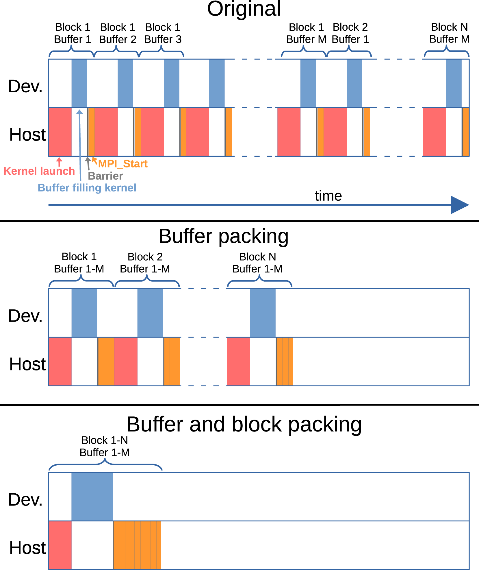
The second (and more specific to GPU-accelerated simulations) strategy is filling more than one communication buffer in a single kernel. In Athena++ each buffer is filled independently in small pack and unpacking routines. However, the work done in these buffer filling kernels is very small, for example, just copying 8 numbers for a corner buffer of a 3D block with 2 ghost zones in each direction, making the actual kernel runtime significantly smaller than the kernel launch time (typically a couple of μs). Given that some vendor APIs (e.g., when running with the CUDA backend) are inherently serial for launching kernels, no significant performance increase can be expected even when multiple kernels can be executed in parallel on the device. For this reason, we implemented a flexible “fill-in-one” approach that allows us to fill all buffers of one or more Variables on one or more blocks in a single kernel, see Figure 2 for an illustration. The performance in practice of this approach is shown in Section 5.1.
Illustration of the buffer and block packing machinery in Parthenon. (top) In the original refactoring from Athena++ each communication buffer of each block is packed separately and sequentially with the runtime of the kernel typically being smaller than the kernel launch overhead itself. (middle) With buffer packing all communication buffers of a single block are filled in a single kernel (with slightly larger runtime – but more parallelism inside the kernel). (bottom) With buffer packing and block packing all buffers of all blocks in pack (number of blocks per pack is a runtime parameter) are filled in a single kernel (allowing for even more parallelism).
With the block structured AMR adopted in Parthenon, prolongation and restriction of data only occurs during communication of data between neighboring MeshBlocks at different levels of refinement, and therefore these steps are functionally part of the boundary communication design. Data sent from fine-to-coarse levels are first restricted and then communicated to reduce message sizes. Data sent from coarse-to-fine are packed into special coarse buffers on the target MeshBlock. Once all communication has completed, the data in these coarse buffers are then interpolated (prolongated) to the fine resolution. Details of the multi-level communication and interpolation algorithms for cell- and face-centered data are given in Sections. 2.1.3 and 2.1.5 of Stone et al. (2020). Again, in order to reduce the number kernel launches restriction is now handled within the “fill-in-one” machinery in contrast to Athena++ where each restriction is a separate kernel.
Finally, contrary to the Athena++ design each Variable uses a unique MPI communicator rather than the default communicator and individual buffers use MPI tags created sequentially rather than globally. The key advantage is to circumvent the minimum upper bound of at least 32,767 defined by the MPI standard. This bound is easily reached when running 3D mesh refinement simulations with small block sizes on modern devices where a single rank can (computationally) easily handle 100s–1000s of blocks.
3.8. Load balancing and mesh refinement
When new MeshBlocks are created or destroyed as part of the AMR, load balancing of the resulting workload across devices becomes important. Following the strategy in Athena++ (see section 2.1.6 in Stone et al. (2020)), in ParthenonMeshBlocks are redistributed across nodes whenever mesh refinement occurs and the tree is rebuilt. Generally some fractions of the MeshBlocks on each device will have to be moved to neighbors to achieve good balance. Nevertheless, the increase in performance associated with good load balancing outweighs the overhead of this communication. Note that mesh derefinement is only allowed periodically (controlled by a runtime parameter) to prevent regions very close to the criterion from refining and then derefining on subsequent cycles.
For performance, the new tree structure is always rebuilt first and that information is used to determine the meshblock distribution across ranks. Thus, only afterward the tree is populated with data either by (a) moving pointers to MeshBlock objects for same-level, same-rank blocks from the old to the new tree, (b) by creating or destroying blocks for same-rank, (de)refined blocks, or (c) by sending meshblock data to a different rank. For the latter, the data transfer is optimized for size, that is, if blocks can be derefined on the sending rank, this is done first before sending the data, and, similarly, if the block needs to be refined, the original data is being sent and the refinement occurs on the receiving rank.
3.9. IO
Parthenon uses (parallel) HDF5 to read and write simulation data. An arbitrary number of different outputs can be defined for a given simulation that can differ in the time interval for writing output, the variables contained, the precision (single or double precision floating point numbers) and the compression level. The latter is also enabled through the HDF5 library and allows for inline compression, which is particularly useful for sparse variables. Several environment variables are processed by Parthenon for a fine-grained control of both HDF5 parameters as well as MPI-IO parameters. For performance, data locality, and (optional) compression HDF5 chunking is used where each chunk corresponds to the meshblock data of a Variable component. The special “restart” output type forcibly includes all variables with the Independent or RestartMetadata flags and write output in double precision. They allow for a simulation to be restarted in a bitwise identical manner. Moreover, when restarting a simulation a different number of MPI ranks can be chosen, for example, to adapt to a changing number of MeshBlocks when using AMR. This is naturally handled by the load balancing mechanism as the tree is being rebuilt upon restarting a simulation.
Parthenon also automatically writes xdmf files along the data files, which allows external (analysis) tools such as ParaView or VisIt to directly read the output data. Finally, a yt frontend is currently being reviewed and expected to be merged soon.
3.10. Tasks and reductions
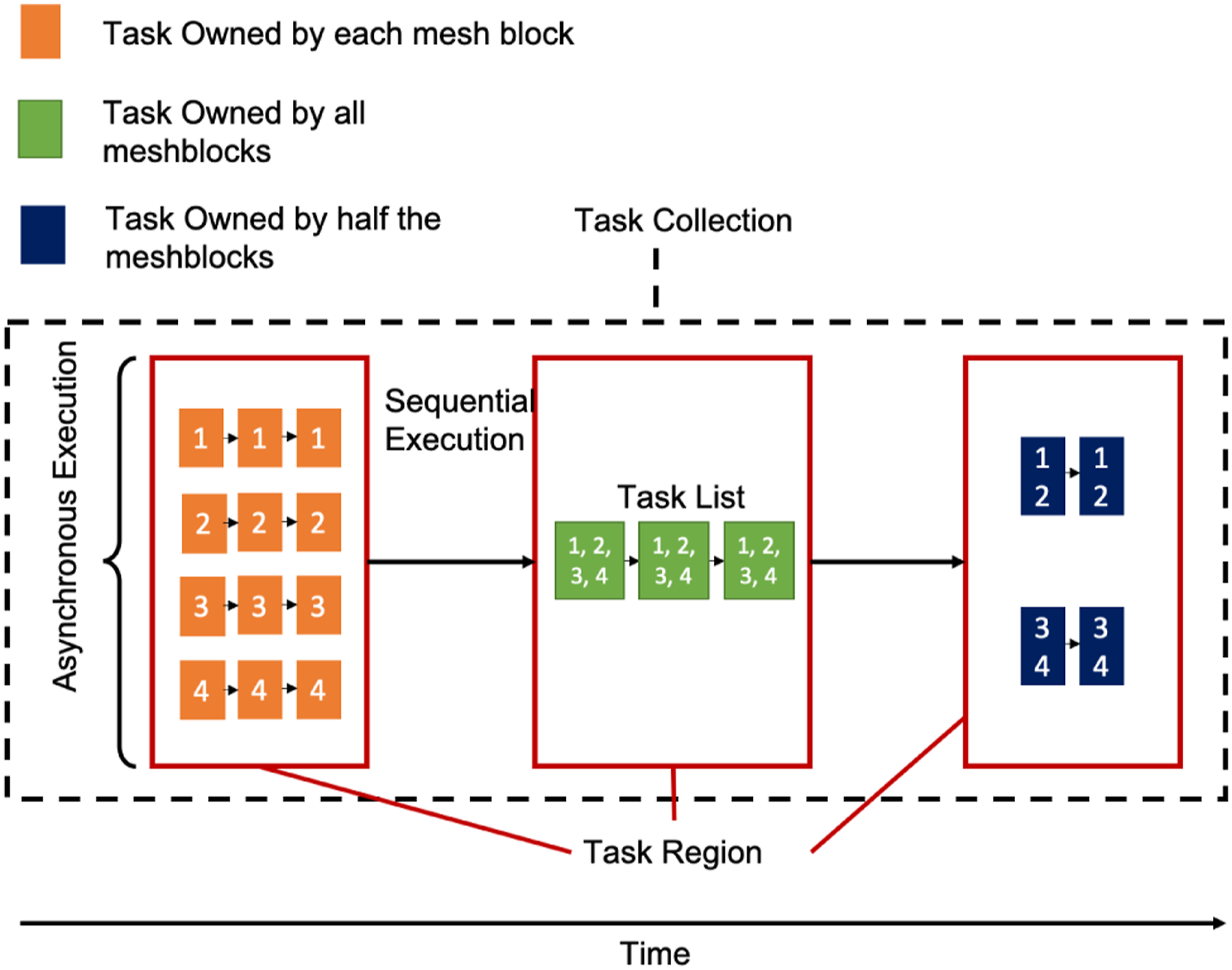
Parthenon provides a simple infrastructure for exploiting task-based parallelism. Tasks are organized hierarchically in TaskCollection, TaskRegion, and TaskList objects. In typical usage, applications build and execute a TaskCollection object that encapsulates each stage of a calculation, which might correspond to a timestep or even a single Runge–Kutta integrator stage. Each TaskCollection is made up of one or more TaskRegions, each of which contains one or more TaskLists. At the lowest level of the hierarchy, tasks are added to TaskList objects by capturing the function to be executed, all of its arguments, and any dependencies that must be executed before the task can be launched. Tasks in a TaskList all operate on data at the same granularity, be that the data on a single “MeshBlock” or data across multiple “MeshBlocks.” Tasks in different TaskList objects within a TaskRegion can be executed concurrently, but TaskRegions are serialized within a TaskCollection. Figure 3 illustrates these relationships.
Tasks are organized into regions which are in turn organized into collections. Task regions within a collection are executed sequentially and each task region can have a different granularity. The illustrated task collection is composed of three task regions, controlling the execution of tasks on four MeshBlocks, indicated by the numbers. The first region launched (potentially) concurrent tasks on each MeshBlock, where the dependencies of a given task can only be other tasks that operate on the same MeshBlock. Once all tasks in the region are complete, the execution moves to the next region where three tasks are launched that each operate on all four MeshBlocks simultaneously. Finally, once these are complete, execution moves to the final region which defines tasks that operate on subsets of MeshBlocks. In this way, task granularity is controlled at the task region level and overall execution is controlled at the collection level.
Many algorithms require the ability to do global reductions. In a task-based environment where each rank may be executing multiple tasks lists operating on independent sub-domains, orchestrating these reductions is nontrivial. Parthenon provides task-based global reductions for typical datatypes encountered in downstream applications such as plain integers or floating point data, std::vectors thereof, and Kokkos::Views or parthenon::ParArrayNDs. Reductions are realized by updating a shared rank-local variable from individual tasks in each TaskList. Those tasks are marked as a shared dependency within that TaskRegion. Only after all tasks with the shared dependency are completed a non-blocking MPI reduction operation is called from a single task on each rank.
3.11. Application driver
In Parthenon-based applications, a driver orchestrates the execution of a computation by building and executing collections of tasks, calling I/O functions as needed, and calling into the load balancing and AMR capabilities, if desired. Parthenon provides a basic set of driver classes from which applications can derive.
At the most basic level, the Driver class gives access to the mesh and I/O capabilities, but assumes nothing about the type of calculation being performed. Downstream applications must define an Execute function that encapsulates the entirety of the control flow and execution. The calculate_pi example demonstrates a capability that derives from Driver, namely, one that approximates the value of π using AMR.
Deriving from Driver, the EvolutionDriver is appropriate for applications that evolve a solution through time. In this case, Execute is already defined. When applications derive from EvolutionDriver they must provide a Step function that is responsible for evolving a solution through a timestep. The EvolutionDriver calls this Step function from within a loop that executes until a specified amount of simulated time has elapsed, calling the I/O, load balancing, and AMR capabilities as appropriate.
Finally, Parthenon provides a MultiStageDriver which derives from the EvolutionDriver, defining the Step function as appropriate for a multi-stage Runge–Kutta integration. In this case, the downstream application need only define a MakeTaskCollection function which must build the TaskCollection object appropriate for a single stage of the integration. The advection example demonstrates the usage of this driver class.
3.12. Machine dependent build configuration
While the hardware environment becomes more heterogenous (requiring performance portable approaches), the software environment similarly adapts and becomes more heterogenous. For example, custom launchers like = jsrun = on OLCF’s Summit are developed and used to allow for an appropriate mapping of hardware resources to processes for parallel execution. At the same time, the user has to choose a suitable mix of compiler, communication, and potentially offloading libraries for configuring, compiling and running a code.
For ease of use, Parthenon ships with so-called machine configuration files for various supercomputers. These files contain default values, e.g. architecture specific flags or parallel launch commands, as well as a recommendation for the environment modules to load. The configurations are regularly tested and updated to reflect the latest software environment provided on a system. This allows (new) users to readily compile and run the test suite without being bothered by machine specific details.
4. Downstream applications
4.1. Parthenon-hydro
Parthenon-hydro1 is a minimal implementation of algorithms solving the Euler equations. In contrast to the examples included in the Parthenon repository, which are mainly used to demonstrate and/or test individual features, Parthenon-hydro is considered a fully-fledged miniapp consisting of just ≈ 1400 lines of C++ code total. Its main purposes are to both illustrate a possible use of various Parthenon features combined in practice as well as an external integration and performance test. Parthenon-hydro supports 1D, 2D, and 3D compressible hydrodynamics on uniform and (static and adaptive) multilevel meshes. Given Parthenon’s Athena++ origins, Parthenon-hydro is also based on a subset of the algorithms implemented in Athena++. More specifically, Parthenon-hydro uses a second-order method consisting of a two-stage Runge–Kutta integrator, piecewise linear reconstruction and HLLE Riemann solver. For illustration purposes following three problem generators are implemented: a linear wave (which is also used to illustrate automated convergence testing by reusing the Parthenon infrastructure externally), a spherical blast wave, and a Kelvin-Helmholtz instability to illustrate adaptive mesh refinement. There are no plans to further extend “physics” capabilities of Parthenon-hydro with the exception of demonstrating new features in Parthenon as hydrodynamics is also supported by other, more feature rich downstream applications such as AthenaPK.
4.2. AthenaPK
AthenaPK (Athena-Parthenon-Kokkos) is a general purpose astrophysical magnetohydronamics code which serves as a performance-portable, AMR-capable conversion of Athena++ (Stone et al., 2020). It implements the hydrodynamics solvers from Athena++ and supplemented them with a divergence cleaning magnetohydrodynamics solver based on Dedner et al. (2002).
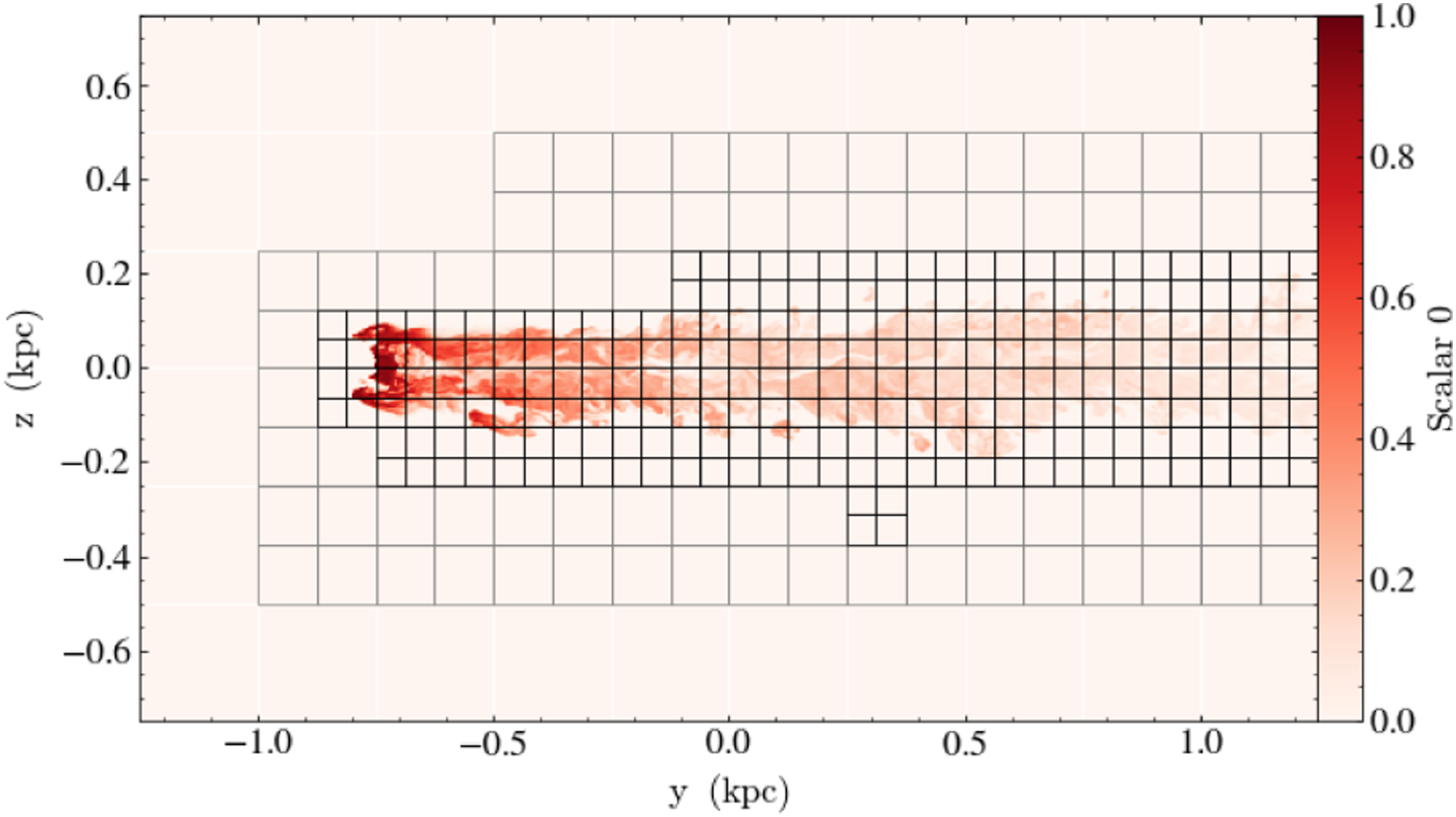
At present, AthenaPK is used for simulations of magnetized galaxy clusters with feedback from active galactic nuclei, cf., Meece et al. (2017); Glines et al. (2020); Prasad et al. (2020), cloud crushing in galatic outflows, and magnetohydrodynamic turbulence. To support these applications additional features implemented include various Riemann solvers, passive scalars, tabulated cooling, and (an)isotropic thermal conduction with support for 2nd-order Runge–Kutta–Legendre based super-time-stepping (Meyer et al., 2014), see Figure 4 for an example multi-physics simulation with AMR.
AthenaPK example: Passive scalar concentration in a supersonic cloud crushing simulation with magnetic fields, optically thin radiative cooling, and mesh refinement configured to follow the cloud material (as passive scalar).
Development of AthenaPK is public and contributions are welcome2.
4.3. Phoebus
Phoebus3 is a general relativistic neutrino radiation magnetohydrodynamics code, designed for modeling compact binary mergers and their aftermath. It uses the Valencia formulation of general relativistic hydrodynamics (Martí et al., 1991), with constrained transport for magnetic fields. Currently the cell-centered formulation of Tóth (2000) is utilized, but face-centered fields will be leveraged once the underlying data structures are implemented in Parthenon. On the radiation side, Phoebus implements Monte Carlo transport as in Miller et al. (2019a), and a novel hybrid scheme first presented in Ryan and Dolence (2020) is in development. Currently Phoebus implements both arbitrary fixed spacetimes as well as self-gravity under the monopole approximation. Full dynamical numerical relativity is a planned improvement. Phoebus carries with it several challenges: a general relativistic background carries with it a very large state vector, with O(100) variables; the fluid primitives are no longer trivially solve-able from the conserved variables, and must be found via numerical root finding; the method requires the interweaving of grid and particle variables; and the general relativistic equations themselves are complicated and compute intensive. A code paper for Phoebus is in preparation.
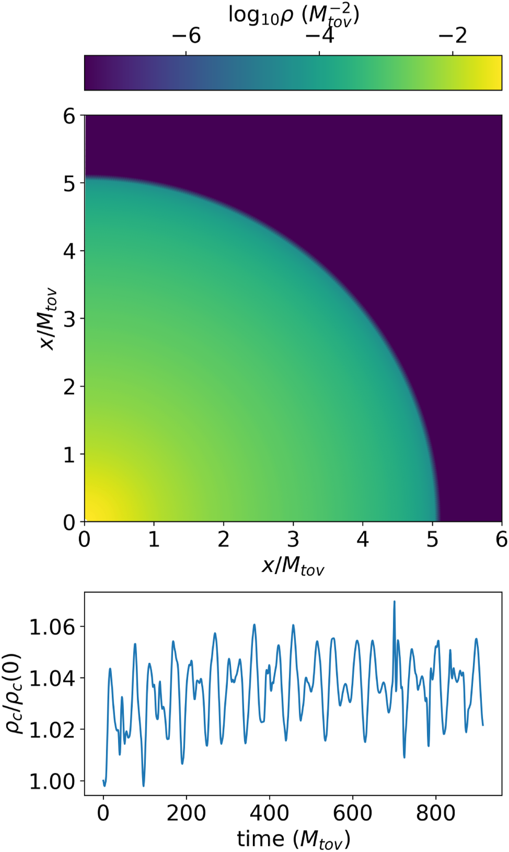
Figure 5 shows an example problem run in Phoebus: a non-rotating neutron star. The top panel shows the density in a poloidal slice. Any small perturbation excites the natural oscillation modes in the star, shown in the bottom panel, where we plot the central density, normalized by its value at the initial time. These modes match those predicted from perturbation theory (Yoshida and Eriguchi 2001) and presented in numerical tests in, for example, Löffler et al. (2012).
Self-gravitating compact star as evolved in Phoebus (top) and oscillations in the central density (bottom). The star is stable for many cycles, and the oscillations match the expected quasinormal mode structure for a non-rotating neutron star.
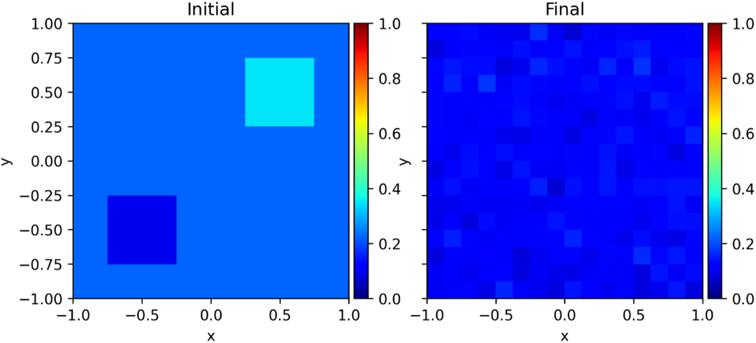
Figure 6 shows another Phoebus example problem using Monte Carlo neutrino transport, leveraging the Parthenon particles infrastructure. In this problem, an initially inhomogeneous electron fraction, the ratio of electrons to baryons, of the background material is homogenized by neutrino emission, transport, and absorption (neutrinos transport lepton number). Inside Phoebus, we use the Singularity-EOS (Miller, 2022a) library for a realistic equation of state (Skinner et al., 2019) and the Singularity-Opac (Miller, 2022b) library for realistic opacities (O’Connor and Ott, 2010; Steiner et al., 2013). Singularity libraries provide production-quality data in a performance-portable way.
Initial and final electron fraction material states of the leptonization neutrino transport problem. Electron fraction-dependent emissivities act to equilibrate the electron fraction across the simulation domain from the inhomogeneous initial conditions. The mean electron fraction of the material is lower at the final time due to the presence of neutrinos.
4.4. RIOT
RIOT is an LANL-based multi-physics code designed to emulate a subset of the physics in the xRAGE code (Gittings et al., 2008) to allow for comparisons of cell-based and block-based AMR approaches. Currently it includes multi-material, compressible hydrodynamics with a pressure–temperature equilibrium mixed-cell closure, gray radiation diffusion, a sub-grid turbulence model, thermonuclear reactions, and high-explosives models. RIOT makes heavy usage of Parthenon’s sparse datatype to represent material based state variables.
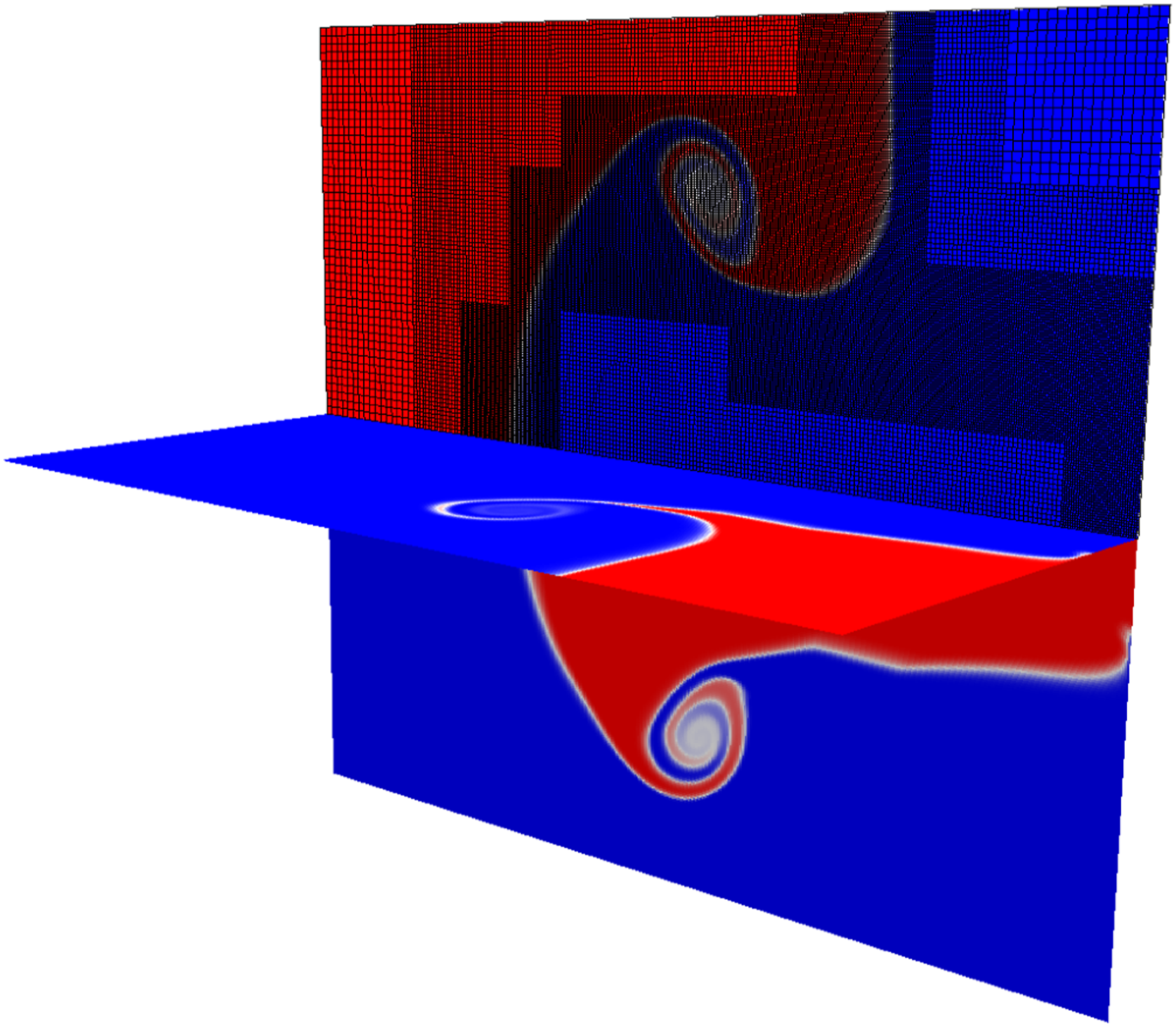
Figure 7 shows results from a classic three material test problem called triple-point (Kucharik et al., 2010). At one end of the domain, an ideal gas at high pressure drives a shock into two distinct ideal gases that differ in their adiabatic index γ. The flow develops vorticity that leads to a well-developed roll-up. The problem was solved in a 3D geometry by revolving the traditional 2D setup about the y-axis and made use of three levels of refinement triggered by material interfaces. The figure shows slices of volume fraction for each material where blue indicates the absence of the material and red indicates a pure material, with white indicating material mixing. On the top slice, we also show the AMR grid to indicate how Parthenon adapts the mesh to accommodate the evolving and nontrivial geometry of the materials.
Slices of material volume fractions in the 3D three material triple-point problem at t = 5.0. Parthenon’s mesh infrastructure enables RIOT to maintain high-resolution around material interfaces, as shown in the top slice.
5. Results
Unless noted otherwise, all result presented in this section were obtained using Parthenon-hydro (changeset 52fa13c with included Kokkos and Parthenon submodules), that is, using a two-stage, second-order method consisting of RK2 integration, piecewise linear reconstruction, and HLLE Riemann solver.
5.1. Block and communication buffer packing
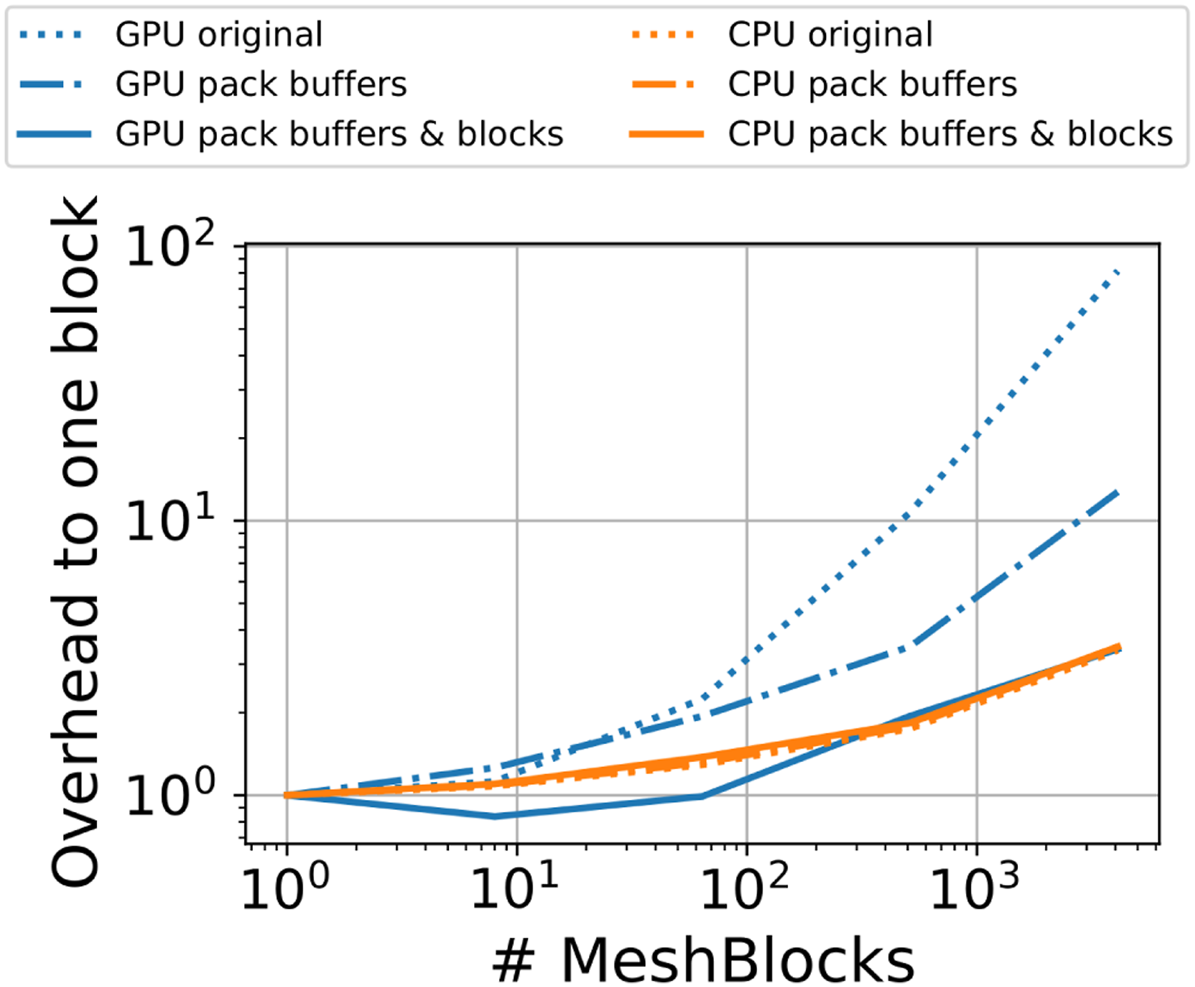
To highlight the need for packing meshblocks and combining the communication buffer filling routines in order to improve the performance on GPUs, we measured the overhead associated with an overdecompositon of the mesh. In this idealized setup, the mesh size is kept fixed and the meshblock size is varied. With smaller and smaller meshblocks, the ratio of ghost cells to active cells increases, the number of buffers increases, and, generally, the overhead associated with managing the entire hierarchy of meshblocks increases. Figure 8 illustrates the relative performance on a single GPU (V100) and a single CPU core (Xeon Gold 6148) when going from using a single meshblock for the entire mesh to 4096 meshblocks.
Overhead associated with an overdecompositon of the mesh measured as relative performance to a second-order MHD update with AthenaPKusing a single meshblock for the entire mesh. The mesh size is fixed to 2563 (1283) and the block size varies from 2563 (1283) to 163 (83) using a single process on a single V100 GPU (single Xeon Gold 6148 CPU core). The dotted lines show the original performance using a single kernel per block and buffer. The dash-dotted lines show the performance packing all communication buffers of a meshblock in a single kernel and the solid lines correspond to using a single kernel to pack all buffers of all meshblocks in a single kernel. Performance on CPUs is effectively independent of buffer and block packing (all CPU lines are on top of each other).
On the CPU this overdecomposition results in an overhead of independent of whether no packing (“original”), packing all buffers of a meshblock in a single kernel, or packing all buffers of all meshblocks in a single kernel is used. This is comparable to the original implementation in Athena++ with an overhead of , cf., Figure 36 in Stone et al. (2020).
On the GPU, the original implementation that launched one kernel per buffer results in a significant overhead and the performance drops by a factor of . This can be attributed to the kernel launch overhead (≈ 5–7 μs on Summit) that is longer than the kernel runtime itself—especially when the communication buffers are small, for example, for small meshblock sizes or for corners (8 cells) in general. To alleviate this bottleneck, we first tried to use multiple streams and launching kernels from multiple threads. While the performance improved with multiple kernels running simultaneously, the results were not satisfactory because the kernel launch itself is inherently serial at the CUDA level. The seconds approach of reducing the number of kernel launches by filling all buffers of a meshblock in one kernel (see Section 3.7) and by packing multiple blocks (see Section 3.6) significantly reduced the additional overhead. As shown in Figure 8, filling buffers in a single kernel reduced the overhead from to at an overdecomposition of 4096 blocks. Combining this with also handling all meshblocks in a single kernel reduced the overhead further down to , which is now on par with the CPU result.
5.2. Pack sizes and overdecomposition
As already noted in the Athena++ method paper (Stone et al., 2020), some (limited amount of) overdecomposition, that is using more than one block per computing device (e.g., a CPU core) resulted in higher performance as it allowed for additional overlapping of computation and communication. However, with an increasing number of blocks per device the block size itself decreases resulting in a smaller ratio of active to ghost cells that need to be communicated. Thus, an optimal mesh decomposition is problem and hardware dependent.
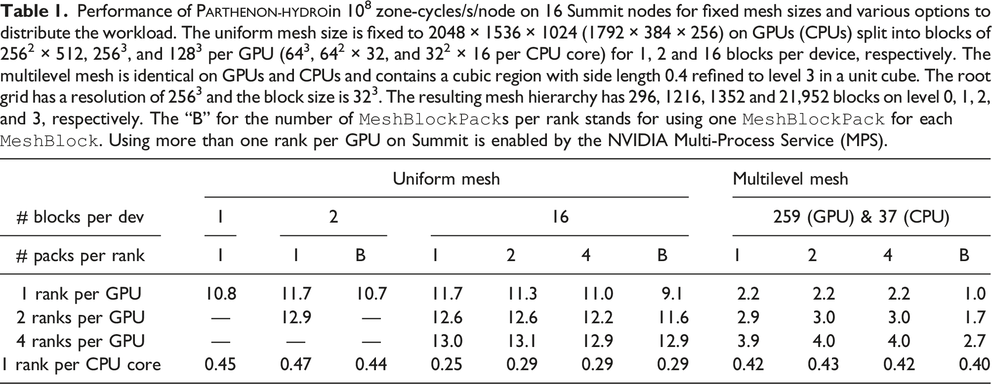
For Parthenon with support for running on GPUs and packing multiple blocks into a MeshBlockPack that are handled simultaneously, finding an optimal decomposition is even more complex. This is illustrated in Table 1 where we list the performance per node of Parthenon-hydro for uniform and multilevel mesh runs on 16 Summit nodes for various options to distribute the workload. Note, the example mesh and block sizes are chosen to illustrate a general direction and details will vary with other factors including (but not limited to) devices (and their features), interconnects, mesh hierarchy, or block sizes.
Performance of Parthenon-hydroin 108 zone-cycles/s/node on 16 Summit nodes for fixed mesh sizes and various options to distribute the workload. The uniform mesh size is fixed to 2048 × 1536 × 1024 (1792 × 384 × 256) on GPUs (CPUs) split into blocks of 2562 × 512, 2563, and 1283 per GPU (643, 642 × 32, and 322 × 16 per CPU core) for 1, 2 and 16 blocks per device, respectively. The multilevel mesh is identical on GPUs and CPUs and contains a cubic region with side length 0.4 refined to level 3 in a unit cube. The root grid has a resolution of 2563 and the block size is 323. The resulting mesh hierarchy has 296, 1216, 1352 and 21,952 blocks on level 0, 1, 2, and 3, respectively. The “B” for the number of MeshBlockPacks per rank stands for using one MeshBlockPack for each MeshBlock. Using more than one rank per GPU on Summit is enabled by the NVIDIA Multi-Process Service (MPS).
# blocks per dev
Uniform mesh
Multilevel mesh
1
2
16
259 (GPU) & 37 (CPU)
# packs per rank
1
1
B
1
2
4
B
1
2
4
B
1 rank per GPU
10.8
11.7
10.7
11.7
11.3
11.0
9.1
2.2
2.2
2.2
1.0
2 ranks per GPU
—
12.9
—
12.6
12.6
12.2
11.6
2.9
3.0
3.0
1.7
4 ranks per GPU
—
—
—
13.0
13.1
12.9
12.9
3.9
4.0
4.0
2.7
1 rank per CPU core
0.45
0.47
0.44
0.25
0.29
0.29
0.29
0.42
0.43
0.42
0.40
When using a single MPI rank per GPU the best performance is typically achieved when using just a single pack on each device containing all blocks. Moreover, in the uniform mesh case overdecomposing the mesh into 2 blocks per device increases performance from 10.8 × 10⁸ zone-cycles/s/node to 11.7 × 10⁸. This also holds for using 16 blocks per device on GPUs as the ratio of active to ghost cells is still large for block size of 1283. In contrast, using 16 blocks per CPU core significantly reduces this ratio as the block size is reduced to 322 × 16 in the example given and the performance drops by ≈ 50% compared to using 2 blocks per CPU core, which is optimal (and similar to Athena++).
On GPUs the performance can be improved even further when using more than one rank per device. However, this needs to be supported by the GPU driver or software as the Kokkos programming model currently supports a single device per process only. Both for the uniform and the multilevel mesh the performance is highest when using 4 ranks per device and splitting all blocks on each rank into two packs. On the uniform mesh, it peaks at 13.1 × 10⁸ zone-cycles/s/node and for the multilevel mesh at 4.0 × 10⁸. In contrast, the performance for the multilevel mesh is 4× lower when using a single rank per GPU handling 256 blocks each and using a separate pack for each block. In other words, both packing (i.e., reducing the number of kernel calls) and using more ranks per device (i.e., reducing the number of blocks per rank and, in turn, the block management overhead per host rank) each result in a performance increase of about 2× in this scenario. These potential performance gains/losses related to runtime parameters should encourage problem and application specific tuning for an optimal use of available computational resources.
5.3. On-node performance portability
To highlight the performance portability enabled at the higher level by the intermediate abstraction layer in Parthenon and at the lower level by Kokkos, we measured the performance of Parthenon-hydro on individual devices across several architectures. These include x86 CPUs with AVX2 and AVX512 instruction sets, ARM CPUs with A64FX architecture, NVIDIA GPUs and AMD GPUs.
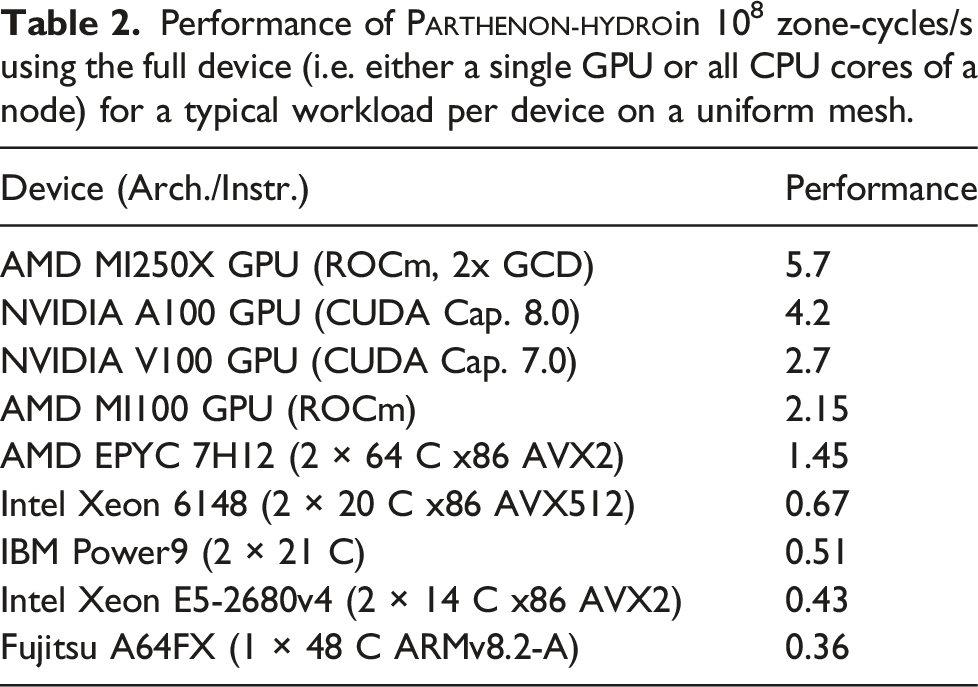
The results are shown in Table 2. A single V100 GPU is about 4× faster than a 40 core Intel Skylake system or faster than a 28 core Intel Broadwell system, which matches the ratios measured for K-Athena (Grete et al., 2021a). Similarly, the Intel CPU performance of Parthenon-hydro only about 20% lower than reported for the same algorithms in Athena++ (Stone et al., 2020) highlighting the low overhead of the abstractions provided by Parthenon.
Performance of Parthenon-hydroin 108 zone-cycles/s using the full device (i.e. either a single GPU or all CPU cores of a node) for a typical workload per device on a uniform mesh.
Device (Arch./Instr.)
Performance
AMD MI250X GPU (ROCm, 2x GCD)
5.7
NVIDIA A100 GPU (CUDA Cap. 8.0)
4.2
NVIDIA V100 GPU (CUDA Cap. 7.0)
2.7
AMD MI100 GPU (ROCm)
2.15
AMD EPYC 7H12 (2 × 64 C x86 AVX2)
1.45
Intel Xeon 6148 (2 × 20 C x86 AVX512)
0.67
IBM Power9 (2 × 21 C)
0.51
Intel Xeon E5-2680v4 (2 × 14 C x86 AVX2)
0.43
Fujitsu A64FX (1 × 48 C ARMv8.2-A)
0.36
On a single MI250X GPU (using 2 GCDs) Parthenon-hydro is about 2.6× faster than on a MI100 GPU and on an A100 GPU Parthenon-hydro is about 55% faster than on a V100 GPU. This corresponds to the increased memory bandwidth in combination with the bandwidth limited algorithms implemented, cf., the roofline model shown in Grete et al. (2021a). While the relative performance of the MI100 GPU with of a V100 GPU is still reasonable (despite the 57% increase in memory bandwidth), the A64FX CPU ( of a V100) is slower than expected based on the device memory bandwidth. First tests indicate that some fraction of the lower performance can be attributed to difficulties of the compiler to (auto)vectorize the compute kernels, which is in agreement with similar results reported for the Flash code (Feldman et al., 2022), and, thus, not intrinsic to the Parthenon framework itself.
5.4. Scaling results
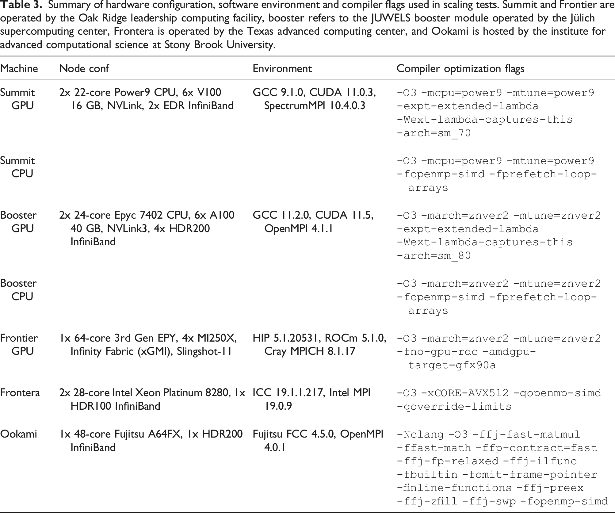
All scaling tests in this subsection have been performed with Parthenon-hydro. Given the simplicity of the algorithms in the miniapp, Parthenon-hydro is a well-suited proxy to gauge the performance of the Parthenon framework itself. Table 3 lists an overview of the node configuration, software environment, and compiler flags of all machines used for testing.
Summary of hardware configuration, software environment and compiler flags used in scaling tests. Summit and Frontier are operated by the Oak Ridge leadership computing facility, booster refers to the JUWELS booster module operated by the Jülich supercomputing center, Frontera is operated by the Texas advanced computing center, and Ookami is hosted by the institute for advanced computational science at Stony Brook University.
Note that the individual mesh sizes used in the scaling tests on uniform meshes vary slightly between different machines and devices. We tried to keep the comparison as fair as possible by ensuring that the computational load per compute element is uniformly distributed, for example, each compute element (a CPU core or a GPU) handles the same number of MeshBlocks for a given test case so that there is no artificial load imbalance. Finally, the numbers reported correspond to the median performance of several tens of cycles to mitigate external effects (such as network congestion) as most of data was collected using non-exclusive allocations.
5.4.1. Weak scaling on uniform grids
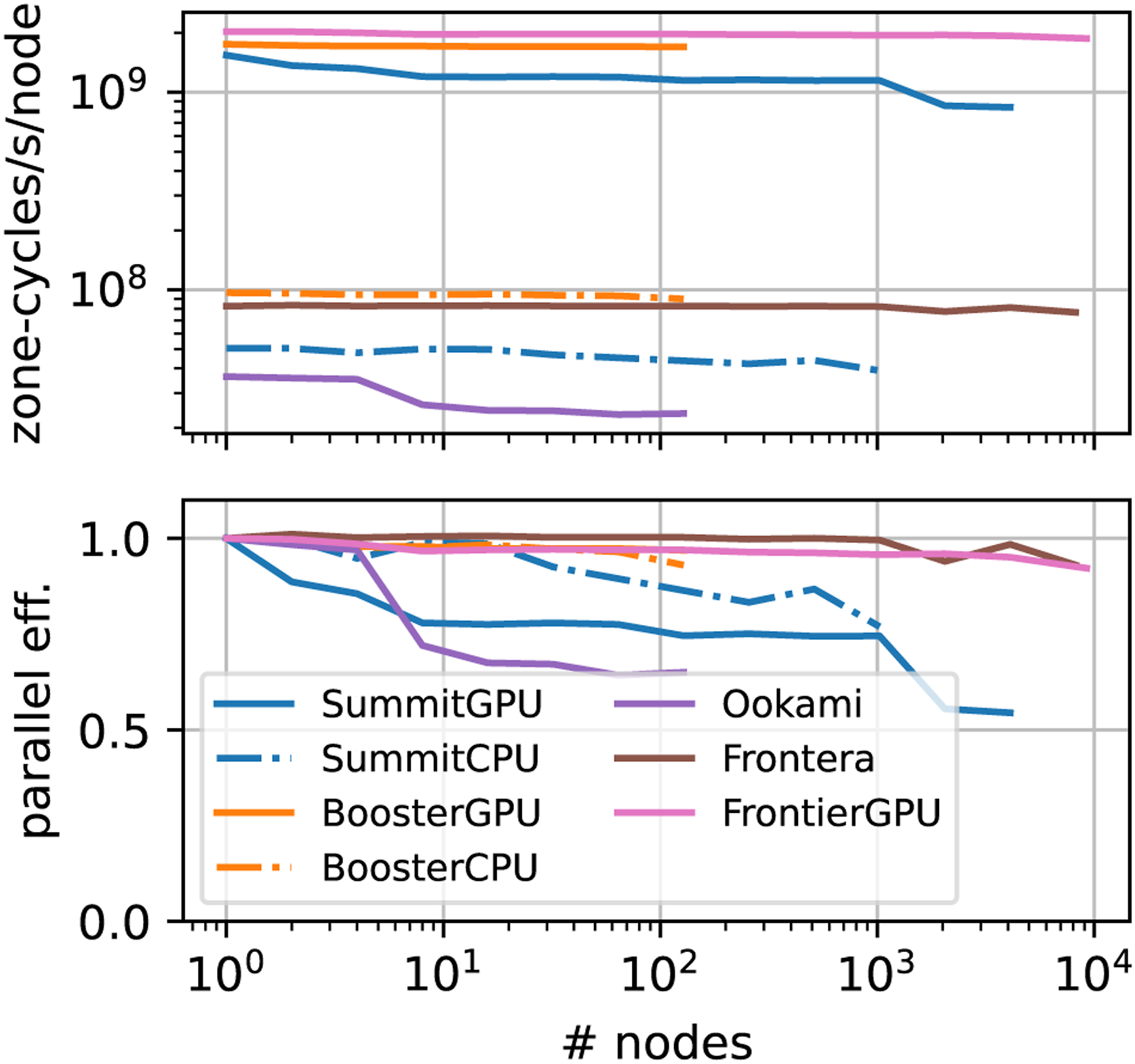
The weak scaling of Parthenon-hydro on various machines is illustrated in Figure 9. In general, we used problem sizes that used a large fraction of the available GPU memory (512 × 2562 per 16G V100 GPU, 5122 × 256 per 40G A100, and 5123 per 64G MI250X GCD) and 643 per CPU core. At the largest scale, Parthenon-hydro reaches a 92% parallel efficiency going from one to 9216 nodes (73,728 logical GPUs) on Frontier for a total of 1.7 × 10¹³ zone-cycles/s—in other words, effectively updating a 16, 3843 mesh about four times per second. At the largest rank count, Parthenon-hydro reaches a 93% parallel efficiency going from one to 8192 nodes (458,752 MPI ranks with one rank per core) on Frontera. Overall, we see a significant speedups using GPUs over CPUs even at large node counts, for example, on a 1024 Summit nodes. In addition, the parallel efficiency is generally comparable between CPUs and GPUs with the exception of Summit. This is in agreement with the scaling behavior of K-Athena (Grete et al., 2021a) and can be attributed to the improved node design of more recent machines. On Frontier and JUWELS Booster each GPU is directly connected to a separate interconnect card, whereas on Summit six GPUs share two InfiniBand cards per node connected to the CPU.
Weak scaling of Parthenon-hydro on uniform grids on various supercomputers with raw performance in zone-cycles per second per node (top), parallel efficiency (bottom). On Summit GPUs (CPUs) on each node handled approximately 5863 (2223) cells, on JUWELS Booster 8123 (2333), on Ookami 2333, on Frontera 2453, and on Frontier 10243, respectively.
5.4.2. Strong scaling on uniform grid
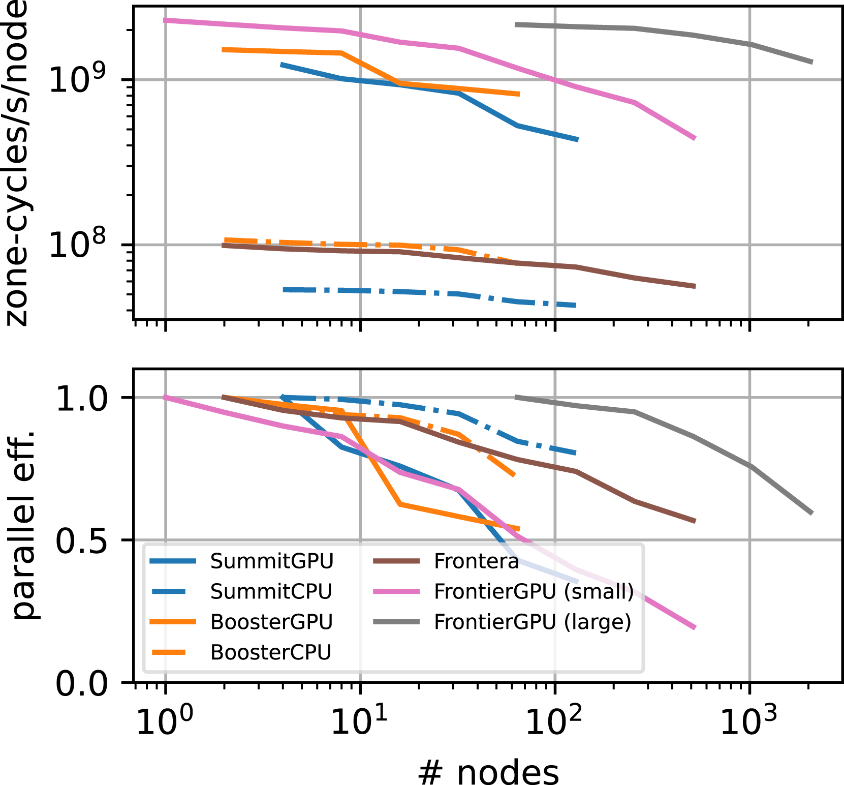
The strong scaling on uniform grids of Parthenon-hydro on various machines is illustrated in Figure 10. We used comparable problem sizes of ≲ 1, 0243 and started with the minimum number of nodes required on each machine. In general, the parallel efficiency using CPUs is slightly higher than using GPUs on the same machine, for example, on Summit remaining at on CPUs for a 32× increase in node count (going from 4 to 128 nodes). While the parallel efficiency on Summit drops to at 128 nodes using GPUs the raw performance of the GPU accelerated simulations is still more than 10× greater than using CPUs. The differences between CPU and GPU strong scaling parallel efficiency can be attributed to the significantly larger ratio of throughput and memory bandwidth to problem size on GPUs, resulting in a more challenging baseline on GPUs, cf., similar results for K-Athena (Grete et al., 2021a). Nevertheless, for a 32× increase in node count on Frontier the parallel efficiency remains high at 67% and 60% going from 1 to 32 or 64 to 2048 nodes, respectively.
Strong scaling of Parthenon-hydroon uniform grids on various supercomputers with raw performance in zone-cycles per second per node (top), parallel efficiency (bottom). On Summit GPUs (CPUs) the mesh size was fixed to 10242 × 768 (1024 × 896 × 768) and the load per node varied from 5863 to 1853 (5613 to 1773). On JUWELS Booster GPUs (CPUs) the mesh size was fixed to 10243 (10242 × 768) and the load per node varied from 8133 to 2563 (7383 to 2363). On Frontera the mesh size was fixed to 10242 × 896 and the load per node varied from 7773 to 1223. On Frontier the small (large) mesh size was fixed to 10243 (40963) and the load per node varied from 10243 to 1283 (10243–3223).
5.4.3. Strong scaling with multilevel grids
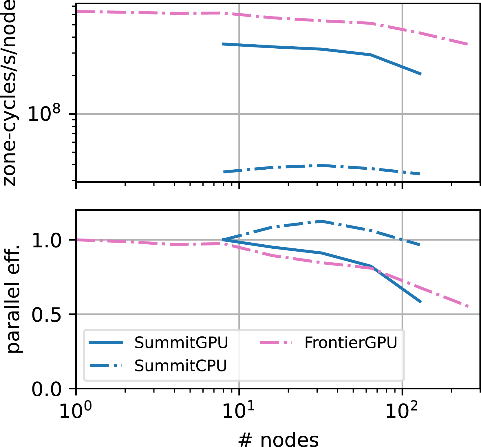
In contrast to the scaling tests on uniform grids presented in the previous two subsections, Figure 11 show the strong scaling behavior of Parthenon-hydro for a multilevel grid. The grid is the same as used in Section 5.2, that is, a block size of 323 is used on a 2563 root grid with 3 additional levels of refinement resulting in 296, 1216, 1352, and 21,952 blocks on level 0, 1, 2, and 3, respectively. Therefore, this tests now includes the prolongation/restriction machinery for ghost zones across level boundaries as well as flux correction for faces across level boundaries.
Strong scaling of Parthenon-hydroon multilevel grids on Summit with raw performance in zone-cycles per second per node (top), parallel efficiency (bottom). The mesh is identical to the one presented in Section 5.2 , i.e. a 2563 root grid with 323 blocks and 3 additional levels of refinement resulting in 296, 1216, 1,352, and 21,952 blocks on level 0, 1, 2, and 3, respectively.
The strong scaling parallel efficiency on CPUs is generally better than on GPUs on Summit reaching and , respectively, going from 8 to 128 nodes. Again, simulations on GPUs are significantly faster than ones using CPUs, but the speedup is lower than on uniform grids, for example, on 8 nodes and on 128 nodes for the given setup. This difference stems from the small kernels sizes, for example, in the flux correction step, which currently is still follows a “one kernel per face” approach, and the associated overhead. We expect further improvements by also using the packing approach described in Section 3.6 for the flux correction. The (limited) super-linear speedup observed in the CPU runs on Summit can be attributed to the mesh management overhead where at the smallest scales (8 nodes) each rank handles ≈ 74 blocks, which is successively reduced with larger rank count, cf., Section 5.1 and 5.2. On GPUs this is not observed as the overhead is hidden by asynchronously running kernels over larger packs of blocks. Finally, on Frontier a 256× increase in resources still results in a parallel efficiency of 55% again highlighting the importance of the direct connection between interconnect and GPUs.
6. Software engineering
6.1. Development model
Parthenon is an open, community-driven effort to create a performance-portable AMR framework applicable for a wide variety of applications. Developers come from several institutions, have access to different computational resources, and have different application needs. In order to meet the needs of disparate interests within the community, we enforce sustainable collaborative software practices. These are also documented in the repository itself in the development guide.
Collaborative development is facilitated via the Parthenon repository on GitHub4. Each contribution to the developmental branch is verified with a continuous integration pipeline, and reviewed and approved by developers from multiple downstream applications. A consistent code style is strictly enforced across the code base with each contribution using automated code style checking and formatting.
New features to the AMR framework are documented and demonstrated in examples contained within the repository. These examples are then used in continuous integration testing.
6.2. Testing
At the highest level, Parthenon uses a ctest-based testing environment that handles various test cases. A shorter test suite is triggered automatically for new commits and/or opened pull request. An extended test suite is executed nightly for the develop branch or be triggered manually. Similarly, the test suite can also be triggered locally during development and offers flexible options to adapt to local environments, for example, with respect to the number of GPUs per node or the MPIlaunch command. The test infrastructure contains the following three building blocks.
6.2.1. Simple, standard tests include unit testing, build testing, and coding style
For each new feature, developers are encouraged to provide separate unit tests that are ideally independent of other components in Parthenon. Parthenon uses Catch2 for these tests to automatically create descriptive test cases that integrate with ctest.
Given the various hardware architectures Parthenon targets and their respective recommended compilers, the automated build testing covers several combinations. These include Release and Debug builds for NVIDIA GPUs with nvcc, x86 CPUs with G++, and AMD GPUs with hipcc. The builds are tested in docker containers that are maintained and published through the main repository so that they are easily available for developers and users.
Finally, consistent code style is automatically enforced using clang-format and cpplint.
6.2.2. Regression tests
Regression tests also include integration tests as they cover more complex use cases. The majority of regression tests use the examples available in Parthenon to verify correctness either against the analytic/exact solution or against a good known previous reference solution.
In contrast to the simple tests, which are directly called from ctest, we development a Python based framework for the regression tests. This framework allows to create complex tests that are tailored to Parthenon, for example, with respect to calling a Parthenon based executable (i.e., one of the examples) with a given input file. The latter can also be modified from within the testing framework. Moreover, the “analysis” step of each test case also allows to process the test results (including the data written to disk or the terminal output) to create artifacts for easy visual inspection.
The testing framework is fully documented and can easily be reused in downstream codes. This allows for a seamless integration of Parthenon and downstream code testing with a unified approach.
6.2.3. Performance testing
Performance testing and reporting is also realized through a separate framework: the Parthenon Performance Metrics App (PPMA). It is a custom GitHub application whose source is maintained in the main repository. It allows to run multi-node performance regression tests on internal machines and can only be triggered manually manually after code review for security reasons. For each run jsonfile is created containing information about time and date of the test, the branch, the commit hash, and various performance metrics. The results are automatically compared and plotted against the previous five commits of that branch and against develop.
7. Current limitations and future enhancements
In the active, ongoing development of Parthenon, we already identified several areas and features that can be further improved and/or need to be implemented motivated by a downstream code requirement.
For example, Parthenon itself currently only supports Cartesian coordinate systems with fixed mesh spacing. Nevertheless, all coordinate related functions are already abstracted and contained in in a separate class. Similarly, all functions provided by Parthenon are already making use of those abstraction, for example, when calculating the divergence of a flux or during flux correction in simulations with mesh refinement. Therefore, the addition of other coordinate systems is straightforward.
Similarly, the Variables class is already prepared to handle additional variable types such as face centered or edge centered variables. While basic support for face variables is already implemented (covering allocation and index handling), the boundary and communication routines are not fully refactored yet.
From a performance point of view, we are currently evaluating further improvements in the ghost zone communication routines. For example, while overlapping computation and communication is already supported through the tasking infrastructure in combination with asynchronous MPI routines, all ghost zones are currently handled in the same way. This is not ideal as ghost zones with neighbors on the same rank, that is, ones that are directly copied to the receiving buffer, are handled in the same kernels as those who are first copied into a buffer in preparation for being sent via MPI. We expect that a split of the kernel into handling remote ghost zones and rank-local ones separately (in that order) to be more efficient because rank-local buffers would be copied while all remote buffers are already being transmitted. The same pattern also applies to the unpacking of the receiving buffers in reverse order.
Independently, first tests indicate that the optimal loop pattern for these buffer handling kernels depend on many factors including overall simulation setup (e.g., MeshBlock size or ghost zone width), implementation details (e.g., number of components in a Variable vector), or device architecture. The results are not yet conclusive, but we expect to eventually provide both an architecture specific default pattern as well as a general simulation/algorithm dependent guideline. This similarly applies to other runtime parameters such as the default MeshBlockPack size or the number of ranks per device, cf., Section 5.2.
8. Conclusions
In this article, we presented the performance portable block-structured adaptive mesh refinement framework Parthenon. Performance portability is achieved through the use of the Kokkos library in combination with an intermediate abstraction layer. The mesh refinement machinery is based on Athena++.
The overall design philosophy follows a device-resident approach, that is, all simulation data is only allocated on the computing device to reduce data movement. Moreover, Parthenon is designed for shared capabilities between various downstream application codes by exposing granular interfaces to the application developers. At the same time, we strive to keep Parthenon simple enough to be easily extensible.
Key features includes abstractions for packages, which can be considered as disparate components containing, for example, a hydrodynamics solver or a radiation transport solver, abstractions for multidimensional variables including vectors and tensors with support for sparse allocation, and a task-based applications driver with support for asynchronous, dependency-based task execution.
From a performance point of view, the key features include the packing of variables and blocks into larger logical structures so that they can be handled within a single kernel. This is particularly relevant for kernels pertaining to filling communication buffers and when using small block sizes as the number of individual kernel launches can be significantly reduced. Similarly, asynchronous, one-sided MPI communicators are used directly from buffers in device memory to allow for an overlap of compute kernels and data transfer between nodes.
We demonstrated the success of these design decisions and features in various scaling test using the hydrodynamics miniapp Parthenon-hydro reaching a total of 1.7 × 10¹³ zone-cycles/s on 9216 Frontier nodes (73,728 logical GPUs) at weak scaling parallel efficiency (starting from a single node). Moreover, we demonstrated performance portability across different CPU and GPU architectures including AMD and NVIDIA GPUs, Intel and AMD x86 CPUs, IBM Power9 CPUs, and Fujitsu A64FX CPUs. In general, simulations employing GPUs are significantly faster compared to using the CPU resources on the same node for both uniform grids (and weak and strong scaling) as well as for multilevel grids, that is, setups that require prolongation/restriction and flux correction.
Several downstream applications are in active development ranging from compressible magnetohydrodynamics to general relativistic neutrino radiation magnetohydrodynamics to multi-material compressible hydrodynamics exemplifying the diverse application scenarios enabled by Parthenon. In addition, we also introduced the Parthenon-hydro miniapp supporting full 3D compressible hydrodynamics with adaptive mesh refinement using Parthenon’s capabilities in just over 1000 lines of code. This also highlights the use of Parthenon as basis for rapid prototyping and testing of new algorithms.
Finally, we emphasize that Parthenon is an open, collaborative project and that new members/contributions are always welcome!
Footnotes
Acknowledgments
The authors would like to thank the Athena++ team, in particular Kengo Tomida, Kyle Felker, and Chris White for having provided an open, well-engineered basis for Parthenon. We also thank the Kokkos team for their continued support throughout the project and John Holmen for supporting the scaling tests on Frontier. Moreover, we would like to thank Daniel Arndt, Kyle Felker, Max Katz, and Tim Williams for their contribution to this work during the Argonne GPU Virtual Hackathon 2021. Finally, we would like to thank our lovely bots, especially par-hermes, who is a very good bot. This work has been assigned a document release number LA-UR-22-21270.
Declaration of conflicting interests
The author(s) declared no potential conflicts of interest with respect to the research, authorship, and/or publication of this article.
Funding
The author(s) disclosed receipt of the following financial support for the research, authorship, and/or publication of this article: This work was supported by the U.S. Department of Energy through the Los Alamos National Laboratory (LANL). LANL is operated by Triad National Security, LLC, for the National Nuclear Security Administration of U.S. Department of Energy (Contract No. 89233218CNA000001). PG acknowledges funding from LANL through Subcontract No.: 615487. This project has received funding from the European Union’s Horizon 2020 research and innovation programme under the Marie Skłodowska-Curie grant agreement No 101030214. This research used resources of the Oak Ridge Leadership Computing Facility at the Oak Ridge National Laboratory, which is supported by the Office of Science of the U.S. Department of Energy under Contract No. DE-AC05-00OR22725. The authors acknowledge the Texas Advanced Computing Center (TACC) at The University of Texas at Austin for providing HPC resources during the April 2022 Texascale Days. Code development, testing, and benchmarking was made possible through various computing grants including allocations on OLCF Summit and Frontier (AST146), Jülich Supercomputing Centre JUWELS (athenapk), Stony Brook’s Ookami (BrOs091321F), and Michgian State University’s High Performance Computing Center.
ORCID iDs
Philipp Grete
Joshua C. Dolence
Jonah M. Miller
Ben Ryan
Forrest Glines
Galen Shipman
Christoph Junghans
Daniel Holladay
Notes
Author biographies
Philipp Grete is a Marie Skłodowska-Curie Actions Postdoctoral Fellow at the University of Hamburg. Previously, he was a postdoctoral research associate at Michigan State University after he obtained his PhD from the University of Göttingen in 2016. His interdisciplinary research ranges from plasma modeling to turbulence to high-performance computing with an emphasis on performance portability.
Joshua C Dolence is a scientist at Los Alamos National Laboratory where he leads research efforts in computational multiphysics, co-design for advanced architectures, and relativistic astrophysics.
Jonah Miller is an expert in relativistic astrophysics and high-performance computing. He got his PhD from the University of Guelph where he worked at the Perimeter Institute for Theoretical Physics. He is now a scientist at Los Alamos National Laboratory, where he works on performance portability, numerical analysis, and simulations of high-energy and compact object astrophysics such as core-collapse supernovae and neutron star mergers.
Joshua S Brown is a Software Engineer at Oak Ridge National Laboratory. His interest is in accelerating science through the development of quality scientific software and tooling.
Ben Ryan is a staff scientist at Los Alamos National Laboratory. His scientific interests include numerical methods for radiation hydrodynamics and applying those methods to problems in astrophysics, particularly simulations of accreting black holes. For his work as a member of the Event Horizon Collaboration, he shared in the 2020 Breakthrough Prize in Fundamental Physics.
Andrew Gaspar is a former Computer Scientist at Los Alamos National Laboratory who focused on performance portability to GPUs for mission critical simulation codes.
Forrest Glines is a Metropolis Postdoctoral Fellow at Los Alamos National Laboratory, having received his PhD in Astrophysics and Computational Mathematics, Science and Engineering from Michigan State University in 2022. To enable exascale simulations of astrophysical plasmas, he co-developed the AthenaPK code which he uses to study relativistic magnetized jets emitted by supermassive black holes and black hole mergers.
Sriram Swaminarayan is a senior scientist in the Computer, Computational, and Statistical Sciences division at Los Alamos National Laboratory (LANL). During his long career at LANL he has served in both line and project leadership roles. He was instrumental in creation of the Applied Computer Science Group (CCS-7) and served as its first group leader. He has worked extensively on large scale parallel applications. His recent work is focused on modernization of LANL applications with a view towards preparing them for GPUs and other modern architectures.
Jonas Lippuner earned his PhD in Physics from Caltech and he is now a staff scientist at Los Alamos National Laboratory. His background is in computational and nuclear astrophysics and he is the author of the open-source nuclear reaction network SkyNet.
Clell J (CJ) Solomon is a staff scientist at Los Alamos National Laboratory and the current project leader of the Eulerian Applications Project. He is interested in high-performance computing, software engineering pertaining to abstractions and generic code development for scientific libraries, and particle transport methods particularly Monte Carlo methods. CJ Holds a PhD in Nuclear Engineering from Kansas State University.
Galen M Shipman is a Computer Scientist focusing on deep application and architecture co-design at Los Alamos National Laboratory, Los Alamos, NM, USA.
Christoph Junghans is the Group Leader of the Applied Computer Science group at Los Alamos National Laboratory. His research interests span from scientific software development and engineering over molecular dynamics methods to multi-scale simulation techniques. He holds a PhD in Physics from the Max-Planck-Institute for Polymer Research, Mainz, Germany.
Daniel Holladay is a staff scientist at Los Alamos National Laboratory. His professional interests include using performance portability tools to incorporate higher fidelity models into multi-physics codes. He received a PhD in nuclear engineering from Texas A&M University.
James Stone is a professor in the School of Natural Sciences at the Institute for Advanced Study in Princeton, NJ. Previously he was Lyman Spitzer, Jr Professor and chair of the Department of Astrophysical Sciences at Princeton University. Stone’s research interests are in the use of numerical methods to study nonlinear and multidimensional fluid dynamics in astrophysical systems, such as accretion flows onto black holes.
Luke Roberts is a staff scientist at Los Alamos National Laboratory. His research interests span a number of topics in nuclear astrophysics, mainly focusing on core-collapse supernovae and compact object mergers. He holds a PhD from the University of California Santa Cruz.
References
1.
AlcubierreM (2008) Introduction to 3+1 Numerical Relativity. International Series of Monographs on Physics, OUP Oxford. ISBN 9780191548291. https://books.google.com/books?id=-xRREAAAQBAJ
2.
BakosiJBirdRGonzalezF, et al. (2021) Asynchronous distributed-memory task-parallel algorithm for compressible flows on unstructured 3d eulerian grids. Advances in Engineering Software160: 102962. DOI: 10.1016/j.advengsoft.2020.102962. https://www.sciencedirect.com/science/article/pii/S0965997820310085
3.
BergerMJColellaP (1989) Local adaptive mesh refinement for shock hydrodynamics. Journal of Computational Physics82(1): 64–84. DOI: 10.1016/0021-9991(89)90035-1.
4.
BourneMASijackiD (2021) AGN jet feedback on a moving mesh: gentle cluster heating by weak shocks and lobe disruption. Monthly Notices of the Royal Astronomical Society506: 488–513. DOI: 10.1093/mnras/stab1662.
5.
Brummel-SmithCBryanGButskyI, et al. (2019) Enzo: an adaptive mesh refinement code for astrophysics (version 2.6). Journal of Open Source Software4(42): 1636. DOI: 10.21105/joss.01636.
6.
Carter EdwardsHTrottCRSunderlandD (2014) Kokkos: enabling manycore performance portability through polymorphic memory access patterns. Journal of Parallel and Distributed Computing74(12): 3202–3216. DOI: 10.1016/j.jpdc.2014.07.003. https://www.sciencedirect.com/science/article/pii/S0743731514001257. Domain-Specific Languages and High-Level Frameworks for High-Performance Computing
DednerAKemmFKrönerD, et al. (2002) Hyperbolic divergence cleaning for the MHD equations. Journal of Computational Physics175: 645–673. DOI: 10.1006/jcph.2001.6961.
9.
DubeyAAlmgrenABellJ, et al. (2014) A survey of high level frameworks in block-structured adaptive mesh refinement packages. Journal of Parallel and Distributed Computing74(12): 3217–3227. DOI: 10.1016/j.jpdc.2014.07.001. Domain-Specific Languages and High-Level Frameworks for High-Performance Computing.
10.
FederrathCKlessenRSIapichinoL, et al. (2021) The sonic scale of interstellar turbulence. Nature Astronomy5(4): 365–371. DOI: 10.1038/s41550-020-01282-z.
11.
FeldmanCMichalowiczBSiegmannE, et al. (2022) Experiences with porting the flash code to ookami, an hpe apollo 80 a64fx platform. In: International Conference on High Performance Computing in Asia-Pacific Region Workshops, HPCAsia 2022 Workshop, New York, NY, USA, January 2022: Association for Computing Machinery, pp. 72–77. DOI: 10.1145/3503470.3503478.
12.
GittingsMWeaverRCloverM, et al. (2008) The RAGE radiation-hydrodynamic code. Computational Science & Discovery1(1): 015005. DOI: 10.1088/1749-4699/1/1/015005.
13.
GlinesFWO’SheaBWVoitGM (2020) Tests of AGN Feedback Kernels in simulated galaxy clusters. The Astrophysical Journal901(2): 117. DOI: 10.3847/1538-4357/abb08c.
14.
GretePGlinesFWO’SheaBW (2021a) K-athena: a performance portable structured grid finite volume magnetohydrodynamics code. IEEE Transactions on Parallel and Distributed Systems32(1): 85–97. DOI: 10.1109/TPDS.2020.3010016.
15.
GretePO’SheaBWBeckwithK (2021b) As a matter of tension: kinetic energy spectra in MHD turbulence. The Astrophysical Journal909(2): 148. DOI: 10.3847/1538-4357/abdd22.
16.
HolmenJKHumphreyASunderlandD, et al. (2017) Improving uintah’s scalability through the use of portable kokkos-based data parallel tasks. In: Proceedings of the Practice and Experience in Advanced Research Computing 2017 on Sustainability, Success and Impact. New York, NY, USA, July 2017: PEARC17ACM, p. 278. ISBN 978-1-4503-5272-7. 1–27. DOI: 10.1145/3093338.3093388.
17.
KucharikMGarimellaRVSchofieldSP, et al. (2010) A comparative study of interface reconstruction methods for multi-material ale simulations. Journal of Computational Physics229(7): 2432–2452. DOI: 10.1016/j.jcp.2009.07.009. https://www.sciencedirect.com/science/article/pii/S0021999109003891
18.
LöfflerFFaberJBentivegnaE, et al. (2012) The einstein toolkit: a community computational infrastructure for relativistic astrophysics. Classical and Quantum Gravity29(11): 115001. DOI: 10.1088/0264-9381/29/11/115001.
19.
MacNeicePOlsonKMMobarryC, et al. (2000) PARAMESH: a parallel adaptive mesh refinement community toolkit. Computer Physics Communications126(3): 330–354. DOI: 10.1016/S0010-4655(99)00501-9.
MeeceGRVoitGMO’SheaBW (2017) Triggering and delivery Algorithms for AGN Feedback. The Astrophysical Journal841(133): 17pp.
22.
MeyerCDBalsaraDSAslamTD (2014) A stabilized runge–kutta–legendre method for explicit super-time-stepping of parabolic and mixed equations. Journal of Computational Physics257: 594–626 DOI: 10.1016/j.jcp.2013.08.021. https://www.sciencedirect.com/science/article/pii/S0021999113005597
23.
MignoneAZanniCTzeferacosP, et al. (2011) The pluto code for adaptive mesh computations in astrophysical fluid dynamics. The Astrophysical Journal Supplement Series198(1): 7. DOI: 10.1088/0067-0049/198/1/7.
MillerJMRyanBRDolenceJC (2019a) νbhlight: radiation GRMHD for neutrino-driven accretion flows. The Astrophysical Journal Supplement Series241(2): 30. DOI: 10.3847/1538-4365/ab09fc.[
27.
MillerJMRyanBRDolenceJC, et al. (2019b) Full transport model of gw170817-like disk produces a blue kilonova. Physical Review D100: 023008. DOI: 10.1103/PhysRevD.100.023008. https://link.aps.org/doi/10.1103/PhysRevD.100.023008
28.
MillerJMSchnetterE (2016) An operator-based local discontinuous galerkin method compatible with the BSSN formulation of the einstein equations. Classical and Quantum Gravity34(1): 015003. DOI: 10.1088/1361-6382/34/1/015003.
29.
MillerJMSprouseTMFryerCL, et al. (2020) Full transport general relativistic radiation magnetohydrodynamics for nucleosynthesis in collapsars. The Astrophysical Journal902(1): 66. DOI: 10.3847/1538-4357/abb4e3.
30.
MniszewskiSMBelakJFattebertJL, et al. (2021) Enabling particle applications for Exascale computing platforms. arXiv e-prints : arXiv:2109.09056.
31.
O’ConnorEOttCD (2010) A new open-source code for spherically symmetric stellar collapse to neutron stars and black holes. Classical and Quantum Gravity27(11): 114103. DOI: 10.1088/0264-9381/27/11/114103.
32.
PrasadDVoitGMO’SheaBW, et al. (2020) Environmental dependence of self-regulating black Hole Feedback in Massive Galaxies. The Astrophysical Journal905(1): 50. DOI: 10.3847/1538-4357/abc33c.
33.
ResslerSMWhiteCJQuataertE, et al. (2020) Ab initio horizon-scale simulations of magnetically arrested Accretion in Sagittarius A* Fed by Stellar winds. The Astrophysical Journal Letters896(1): L6. DOI: 10.3847/2041-8213/ab9532.
34.
RyanBRDolenceJC (2020) MOCMC: method of characteristics moment closure, a numerical method for covariant radiation magnetohydrodynamics. The Astrophysical Journal891(2): 118. DOI: 10.3847/1538-4357/ab75e1.
35.
RyanBRResslerSMDolenceJC, et al. (2018) Two-temperature GRRMHD simulations of m87. The Astrophysical Journal864(2): 126. DOI: 10.3847/1538-4357/aad73a.
36.
SkinnerMADolenceJCBurrowsA, et al. (2019) FORNAX: a flexible code for multiphysics astrophysical simulations. The Astrophysical Journal Supplement Series241(1): 7. DOI: 10.3847/1538-4365/ab007f.
37.
SteinerAWHempelMFischerT (2013) Core-collapse supernova equations of State based on Neutron star observations. The Astrophysical Journal774(1): 17. DOI: 10.1088/0004-637X/774/1/17.
38.
StoneJMTomidaKWhiteCJ, et al. (2020) The athena++ adaptive mesh refinement framework: design and magnetohydrodynamic solvers. The Astrophysical Journal Supplement Series249(1): 4. DOI: 10.3847/1538-4365/ab929b.
39.
TeyssierR (2002) Cosmological hydrodynamics with adaptive mesh refinement. A new high resolution code called RAMSES. Astronomy and Astrophysics385: 337–364. DOI: 10.1051/0004-6361:20011817.
TrottCLebrun-GrandieDArndtD, et al. (2021) Kokkos 3: programming model extensions for the exascale era. IEEE Transactions on Parallel and Distributed Systems1: 805–817. DOI: 10.1109/TPDS.2021.3097283.
42.
YoshidaSEriguchiY (2001) Quasi-radial modes of rotating stars in general relativity. Monthly Notices of the Royal Astronomical Society322(2): 389–396. DOI: 10.1046/j.1365-8711.2001.04115.x.
ZhangWMyersAGottK, et al. (2021) Amrex: block-structured adaptive mesh refinement for multiphysics applications. The International Journal of High Performance Computing Applications35(6): 508–526. DOI: 10.1177/10943420211022811.