
Abstract
Recently, accelerator hardware in the form of graphics cards including Tensor Cores, specialized for AI, has significantly gained importance in the domain of high-performance computing. For example, NVIDIA’s Tesla V100 promises a computing power of up to 125 TFLOP/s achieved by Tensor Cores, but only if half precision floating point format is used. We describe the difficulties and discrepancy between theoretical and actual computing power if one seeks to use such hardware for numerical simulations, that is, solving partial differential equations with a matrix-based finite element method, with numerical examples. If certain requirements, namely low condition numbers and many dense matrix operations, are met, the indicated high performance can be reached without an excessive loss of accuracy. A new method to solve linear systems arising from Poisson’s equation in 2D that meets these requirements, based on “prehandling” by means of hier-archical finite elements and an additional Schur complement approach, is presented and analyzed. We provide numerical results illustrating the computational performance of this method and compare it to a commonly used (geometric) multigrid solver on standard hardware. It turns out that we can exploit nearly the full computational power of Tensor Cores and achieve a significant speed-up compared to the standard methodology without losing accuracy.
Keywords
1. Motivation and related work
Accelerator hardware, in particular current GPUs equipped with Tensor Cores tailored for AI applications, is an increasingly important component of state-of-the-art computer systems, which is used to boost their computing power. For instance, the NVIDIA Tesla V100 Tensor Core GPU, which we consider in this work, reaches up to 7.8 TFLOP/s in double precision and 125 TFLOP/s in half precision due to the usability of Tensor Cores according to the manufacturer specifications (NVIDIA, 2020). Of course, it is desirable to apply the V100 or similar GPUs in the context of numerical simulation, or more precisely, to solve linear systems resulting from the discretization of partial differential equations (PDEs), for example, via finite element methods (FEM), that are associated with continuum mechanics. But when trying to do so, one encounters the problems explained in more detail in the following two sections, namely the risk of a deteriorating error if low precision is used in conjunction with high condition numbers, and the presence of sparse matrices, for which Tensor Cores cannot be fully utilized. Consequently, the question arises whether it is possible to implement basic components of finite element simulations on modern accelerator hardware while measurably exploiting its high computing power.
Recent work using other methods also addresses this issue. For instance, Oo and Vogel (2020) investigate how profitably the V100 can be used in the context of a mixed-precision approach for Poisson’s equation, that is, an iterative refinement algorithm with a low-precision multigrid preconditioning involving large, sparse matrices and observe a speed-up by a factor of 2.5 when solving the linear system. Since the operations with sparse matrices are memory-bounded, the peak rates of the V100 are not approached. Another recent paper on this subject is a comprehensive survey, that summarizes some of the latest results on mixed-precision numerical (dense and sparse) linear algebra routines (Abdelfattah et al., 2021). Moreover, a mixed-precision iterative refinement solver for dense matrices with a bounded condition number, that employs an LU factorization in low precision, by Haidar et al. (2020) should be mentioned. The algorithm is accelerated by a factor of four to five compared to the completely double-precision method when running on a Tensor Core GPU. For the case of sparse matrices, there are fewer practical results concerning the use of Tensor Cores, which is not surprising given their special suitability for dense linear algebra. Instead, the focus is on format decoupling and compression and their application to preconditioners for iterative solvers and multigrid methods.
An alternative approach is matrix-free methods. In the article by Kronbichler and Ljungkvist (2019), for example, a matrix-free multigrid algorithm to solve Poisson’s equation on NVIDIA’s Pascal P100 GPU is examined and compared with a CPU implementation, resulting in a speedup by a factor of 1.5–2. The advantages of using single precision are highlighted, but this methodology also likely offers little potential for use with Tensor Core GPUs, if using half precision is even a consideration for reasons concerning the conditioning.
The objective of this proof-of-concept study is to develop hardware-oriented algorithms for solving Poisson’s equation in 2D, which is oftentimes a bottleneck in numerical simulations, on current GPUs and to demonstrate that computations can be accelerated by orders of magnitude in comparison to standard methods on standard hardware given by a geometric multigrid method on multicore CPUs while preserving the required accuracy.
2. An example of modern accelerator hardware
We take a closer look at the two sets of hardware compared in this study. On the one hand, the aforementioned NVIDIA Tesla V100 SXM2 as an example of current GPUs offers 7.8 TFLOP/s in double (DP), 15.7 TFLOP/s in single (SP), 31.3 TFLOP/s in half precision (HP), and 125 TFLOP/s in half precision in conjunction with Tensor Cores. The memory bandwidth is 900 GB/s (NVIDIA, 2020). On the other hand, we consider an x64 architecture in the form of the AMD EPYC 7542 CPU with the following specifications: 32 cores per CPU, 128 MB L3-Cache, 1.5 TFLOP/s in double, 3 TFLOP/s in single precision (half precision is not supported) and a memory bandwidth of 205 GB/s (AMD, 2021) representing modern standard computers used in computer centers, for example.
It should be noted that the stated computer performance rates are peak rates. They can be achieved when tasks with very high arithmetic intensity including dense linear algebra (BLAS3 operations) such as direct solvers for linear systems of equations (with typically cubic complexity) are executed. However, finite element discretizations result in very sparse stiffness matrices and thus standard iterative solvers, for example, Krylov (multigrid) methods, particularly require sparse matrix-vector multiplications. Therefore, the computational performance is bounded by the memory bandwidth.
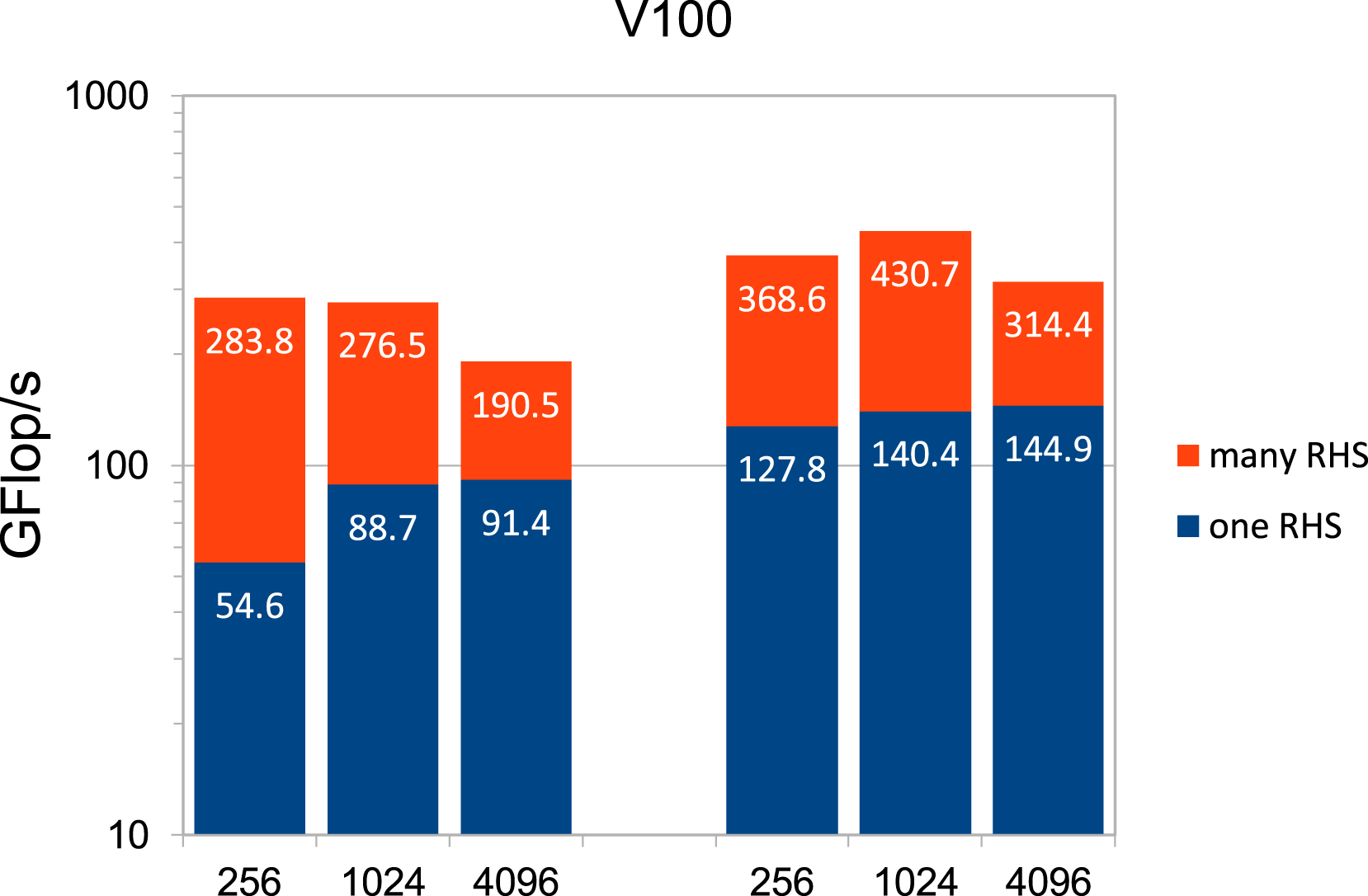
As a test model, we consider Poisson’s equation − Δu = f in 2D on the unit square GFLOP/s for sparse matrix-vector multiplication (one RHS) and sparse matrix-matrix multiplication (many RHS) depending on h−1 in DP and SP (left and right three columns, respectively) on the AMD CPU. GFLOP/s for sparse matrix-vector multiplication (one RHS) and sparse matrix-matrix multiplication (many RHS) depending on h−1 in DP and SP (left and right three columns, respectively) on the V100 GPU.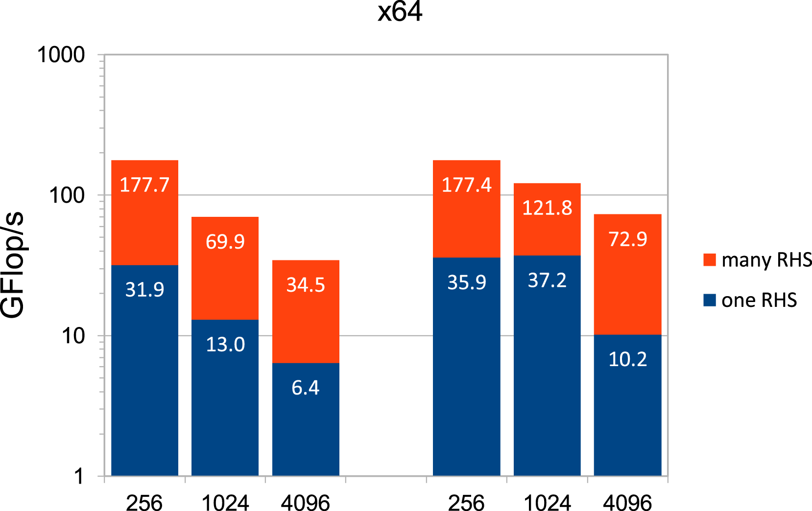
We also remark that our results for optimized matrix-free, more specifically stencil-based, operations on the V100 in the context of a geometric multigrid algorithm show a speedup factor of about 5–10 compared to a CSR approach. Thus, the order of one TFLOP/s is achievable, but this is still far below the peak rate (Poelstra, 2019).
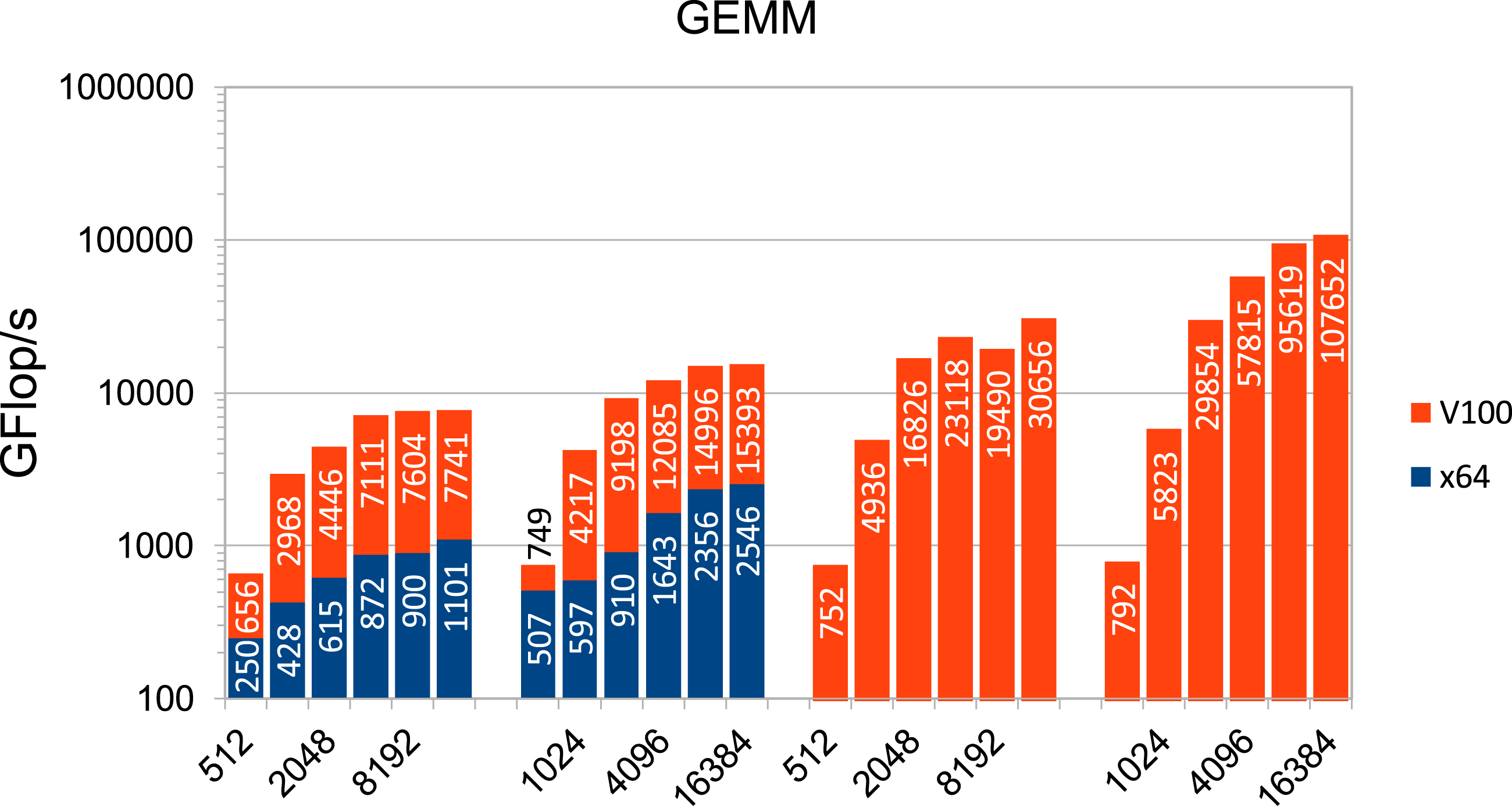
If, instead, one performs calculations with dense matrices, that is, dense matrix-vector and matrix-matrix multiplications, a strong increase in achievable computing power can be observed, as the results shown in Figures 3 and 4 indicate. Note that half precision is not supported on the x64 architecture. The exceptionally high rates in half precision on the Tensor Cores of the V100 demonstrate their performance potential. GFLOP/s for dense matrix-vector multiplication (GEMV) depending on h−1 in DP and SP (first and second set of columns from left, respectively) one the AMD CPU and the V100 GPU. GFLOP/s for dense matrix-matrix multiplication (GEMM) depending on h−1 in DP and SP (first and second set of columns from left, respectively) on the AMD CPU and the V100 GPU and in the case of the V100 in HP without and with Tensor Cores (third and fourth set of columns from left, respectively).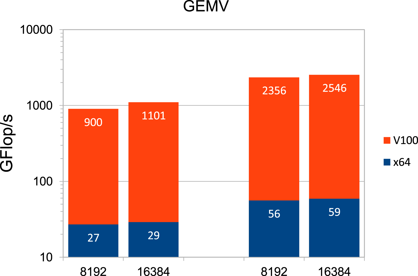
In a nutshell, in this section we have demonstrated the large gap between peak performance on the one hand and actual performance in the setting of finite element applications, that are usually based on sparse matrix-vector operations in double precision, on the other hand. In addition, it has become evident that there is a high potential with regard to numerical simulations of corresponding PDEs in continuum mechanics if low precision, and thus Tensor Cores, as well as dense matrix operations, can be used. To exploit this potential, it is necessary to ensure that the use of low precision does not lead to a significant overall loss of accuracy and to develop solution methods that include dense matrix-vector or matrix-matrix applications.
In the following sections, we pursue both requirements and introduce possible solutions. The next section treats the concept of prehandling (Ruda, 2020; Ruda et al., 2021) for Poisson’s equation, which is an essential component in many numerical simulations. It enables the use of lower precision when solving the linear system with respect to the stiffness matrix while preserving results comparable to those achieved in double precision in terms of accuracy. It can be realized via hierarchical finite elements (Yserentant, 1986) and this approach is then extended to a Schur complement like solution method including multiplications with dense (part) matrices so that Tensor Cores can be fully used. Finally, we provide first numerical results for this particular solver serving as a proof-of-concept that GPUs with Tensor Cores can in fact be appropriately used by means of adjusted hardware-oriented techniques.
3. Prehandling as a concept for stiffness matrices in lower precision
The primary objective of prehandling is to reduce the condition number of the stiffness matrix A
h
corresponding to elliptic PDEs, Poisson’s equation in this case. The necessity will become clear if the following subdivision of the error obtained by a finite element discretization (with mesh width h) given by the difference between the exact solution u and the actual numerical solution

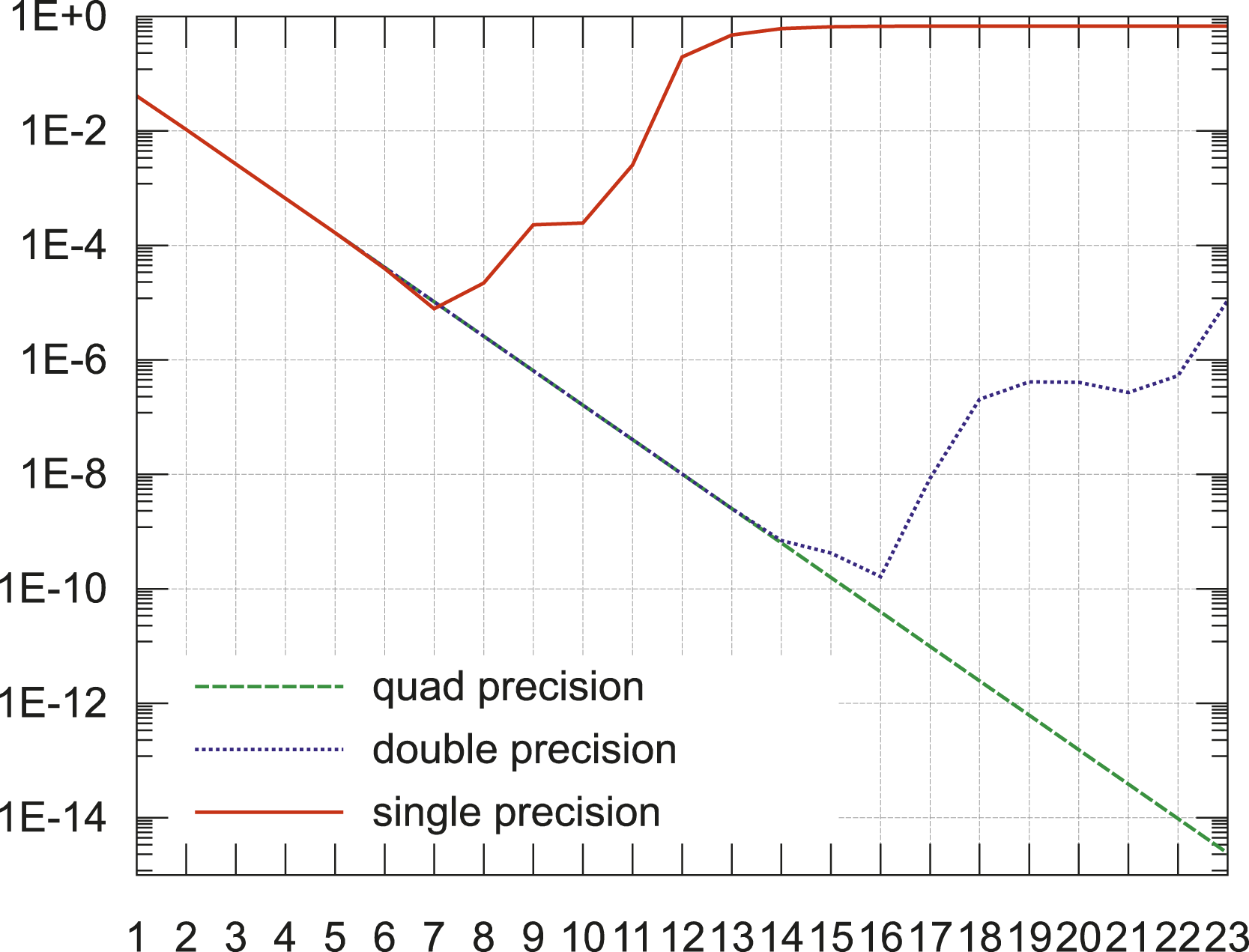
The opposite trends of both error types cause that the mesh width h may not be chosen too small in order to prevent the computational error from becoming dominant. This happens if the mesh width undercuts a certain critical value. In the above example, the intersection of discretization and computational error is at Illustrative course of total, computational, and discretization error in SP in the case of Poisson’s equation with bilinear finite elements. Actual L2-error for single, double, and quad precision with standard finite elements in 1D depending on the refinement level (h = 2−level, so level 10 corresponds to h = 1/1024).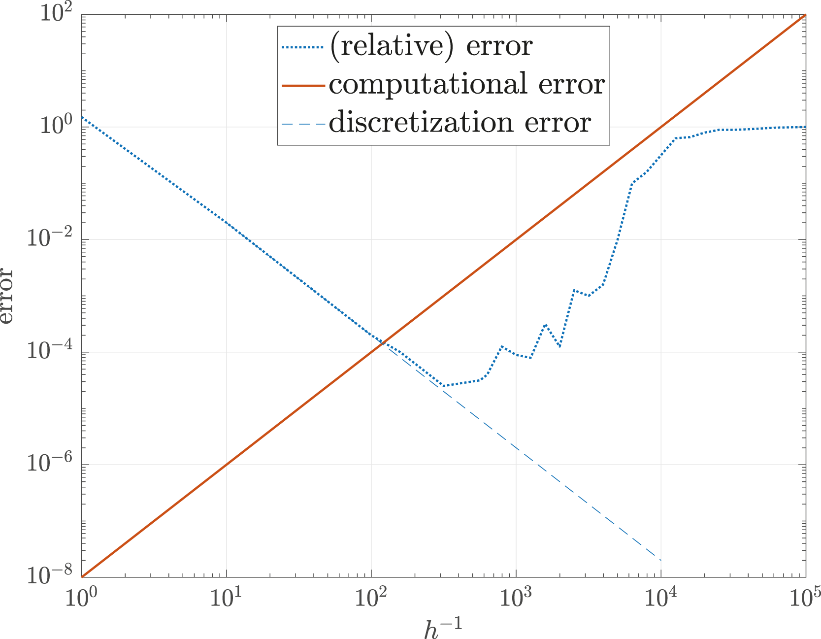
It is desirable to reduce the condition number of the stiffness matrix to widen the range of appropriate grid widths and even allow for the use of lower precision. This can be achieved by explicitly transforming the original linear system A
h
x
h
= b
h
into an equivalent form 1. Strong decrease of the condition number, 2. The matrix 3. The transformation can be realized efficiently (for instance, in
Provided that exact arithmetic is used, solvers in their (implicitly) preconditioned variants would yield the same results as the (explicitly) prehandled forms, but it turns out that the results can differ significantly in finite precision, in particular in case of ill-conditioned stiffness matrices. Well known preconditioners (matrix splitting methods, ILU, SPAI, etc.) that are directly applied to the stiffness matrix are not appropriate options for prehandling since they violate the requirements 1 and 2. The hierarchical finite element method (HFEM) meets the demands for Poisson’s equation, at least in 1D and 2D. Below we outline the basic idea, remarkable properties, and practical aspects of this method.
It was established and analyzed by H. Yserentant et al. in the 1980s, for example, in (Yserentant, 1986). The prerequisite is an initial triangulation (level 0) consisting of triangular or quadrilateral elements that is successively refined yielding a nested sequence of finite element spaces. Here we restrict ourselves to (bi)linear Q1 or P1 finite element discretizations. Instead of a nodal basis, we use a hierarchical basis, which comprises shape functions on each level as shown in Figure 7 in the one-dimensional case. It is straightforward to generalize this idea to higher dimensions. We focus on the two-dimensional case. Left: nodal bases; right: hierarchical bases (only newly added basis functions on the respective meshes) in 1D. Source: Deuflhard et al. (1989).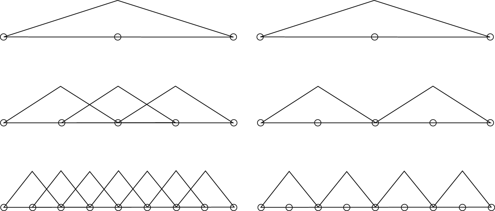
It seems that the assembly of the stiffness matrix and the right-hand side with respect to a hierarchical basis is more complex due to the greater support of the basis functions on lower levels, but it is in fact not necessary to compute them: If the stiffness matrix and right-hand side with respect to a nodal basis are known, we can obtain the respective structures with respect to a hierarchical basis by means of a transformation via the matrix S = S
j
Sj−1…S1. Each factor S
k
in this product corresponds to one step of refinement and can be understood as a typical prolongation from level k − 1 to k as known from geometric multigrid methods. In other words, multiplying a coefficient vector with the matrix S
k
yields the values of the basis functions on the (k‐1)st level at the nodes of the kth level. Hence, the matrices S
k
are identity matrices with additional entries in the rows whose indices correlate with the newly added nodes of level k. In practice, assuming P1 finite elements and uniform refinement of the initial grid (i.e., subdividing each triangle into four congruent triangles), every added level-k-node with index i is adjacent to two level-(k − 1)-nodes, n1(i) and n2(i), so that we have
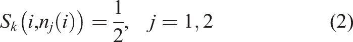
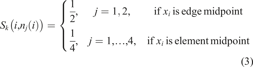
In the case of Q1 finite elements, uniform refinement leads to four edge midpoints with two adjacent nodes on the coarser grid, respectively, and one element midpoint with four adjacent nodes. As a result, the manipulation of the rows of S
k
must be adapted as follows
The arising matrix S is consequently a sparse block unit lower-triangular matrix and the transformed linear system of equations is given as

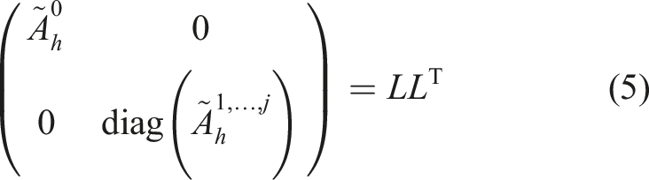
For better results in terms of condition numbers, Yserentant (1986) and Deuflhard et al. (1989) suggest an additional Cholesky decomposition on the initial grid, which can also be directly applied to the stiffness matrix. Let
For both variants, with and without a partial Cholesky decomposition, the remarkable property is that the condition number of the transformed stiffness matrix is asymptotically characterized by
We conducted numerical tests that show that solutions obtained in lower (single or half) precision are considerably more accurate for fine meshes if we use the method of prehandling. An example can be seen in Figure 8. It clarifies that prehandling allows for (in this case) four to five further steps of uniform refinement in half precision without an exceeding loss of accuracy compared to standard finite element methods in double precision. Thus, the use of low precision becomes feasible, at least when solving Poisson’s equation in 2D on hierarchically refined meshes and if a relative accuracy of approximately 1% is acceptable, whereby the latter is a realistic demand in complex technical simulations. L2-errors depending on the refinement level without (dotted graph) and with prehandling via hierarchical finite elements (dashed graph) in HP, respectively, in comparison to the error of the reference solution obtained in DP (solid graph), which is independent of prehandling in this range of levels. A strongly oscillating exact solution to the continuous 2D Poisson problem was chosen. Again, h = 2−level. Note that the error deviates at level 5 without prehandling and at level 8 or 9 with prehandling.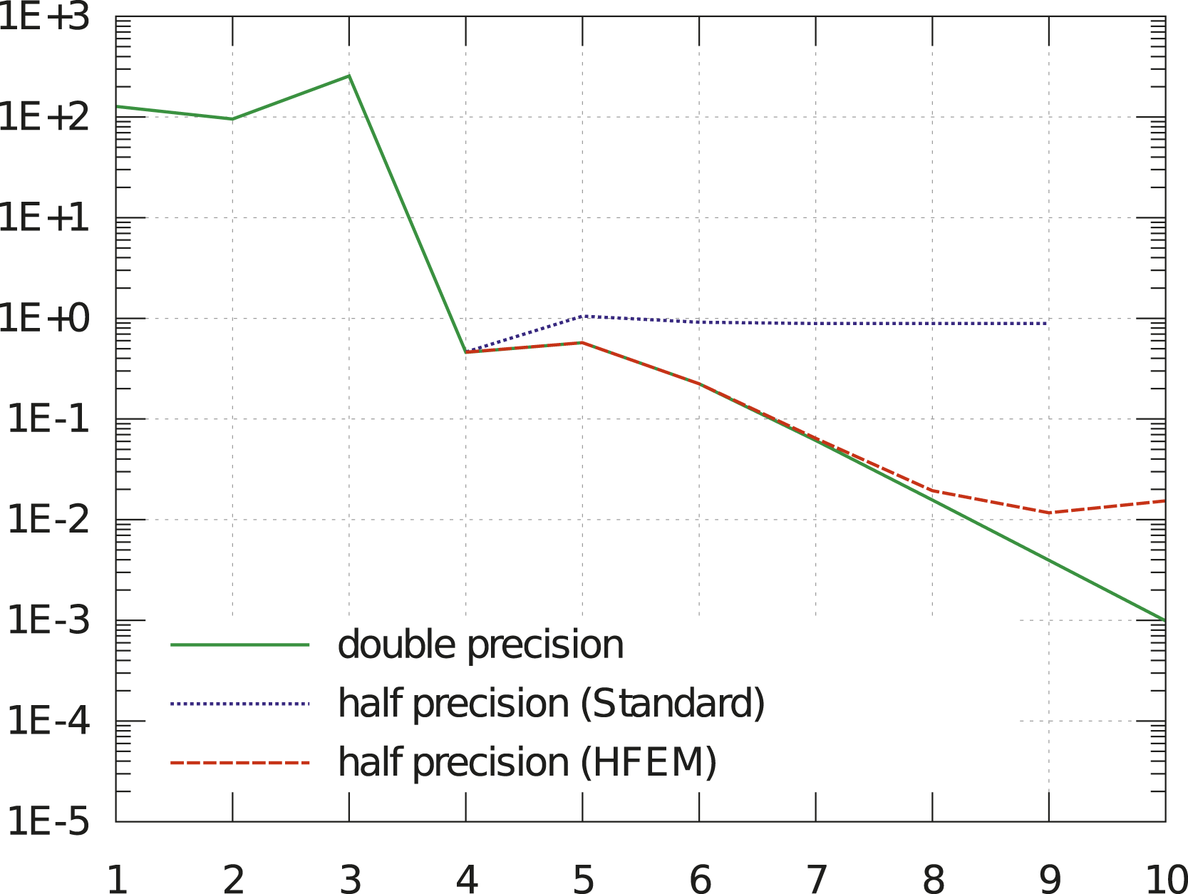
4. Direct solvers based on the HFEM approach
4.1. Derivation of the methods
Let us first take a closer look at the particular structure of hierarchically refined meshes and the consequent structure of stiffness matrices that arise from prehandling via the HFEM approach. Then we derive new solvers tailored for GPUs in low precision. As before, we investigate the case of Poisson’s equation in 2D, discretized with P1 or Q1 finite elements. From now on, for simplicity, we omit the subscript h and assume that
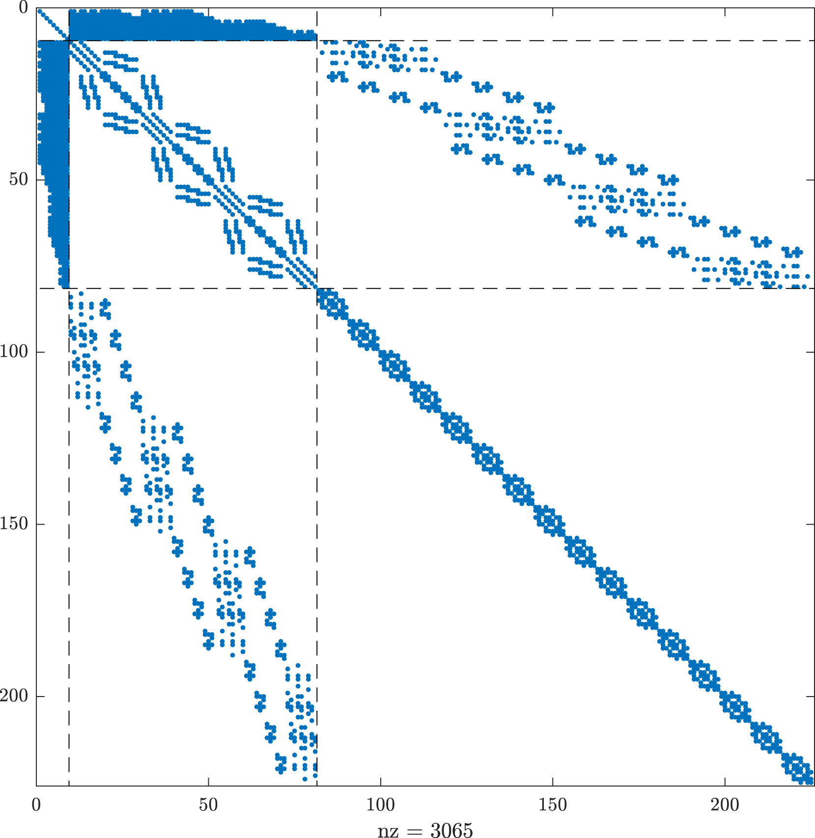
A subdivision of the nodes of the hierarchical mesh and numbering the nodes accordingly yields a special structure of the stiffness matrix that can be exploited to solve the linear system efficiently. We only consider the interior nodes of the discrete domain since nodes on the (Dirichlet) boundary are treated separately. A distinction is made between the following three sets of node indices: • • •
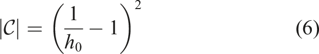
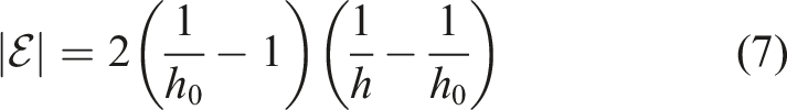
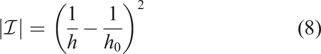
Consequently, Illustration of the three types of nodes on a uniformly refined coarse grid (bold lines) for the unit square with h0 = 1/4 and h = 1/16 and Q1 finite elements. Sparsity pattern of the prehandled stiffness matrix corresponding to the mesh in Figure 9 for the special node numbering.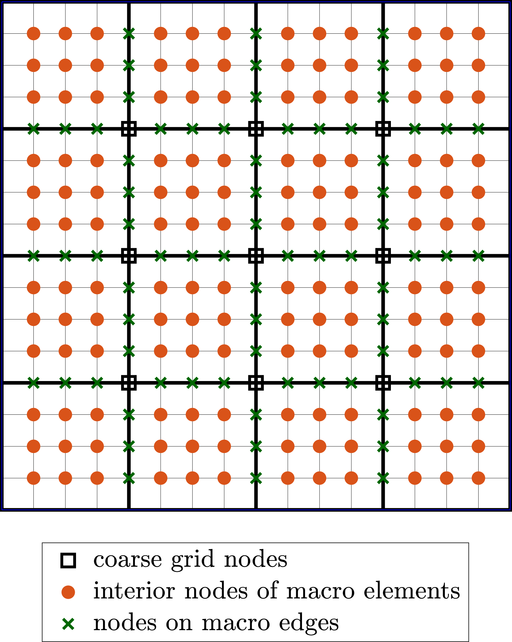
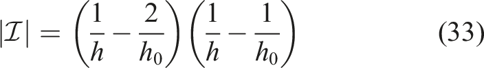
It is worth noting that, when a given coarse grid with width h0 is uniformly refined, the number of interior nodes
Using the notation
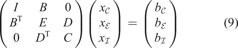


These three subsystems can be rearranged and substituted into each other in several ways, similarly to a Schur complement method for 3 × 3 block matrices. The three resulting different (semi-)direct methods for solving the above system have the potential to exploit the computing power of GPUs in lower precision since dense and well-conditioned matrices and corresponding matrix-vector and matrix-matrix multiplications are involved. As a collective term, we also refer to the methods as PSC methods (Prehandling Schur Complement). They are derived as follows.
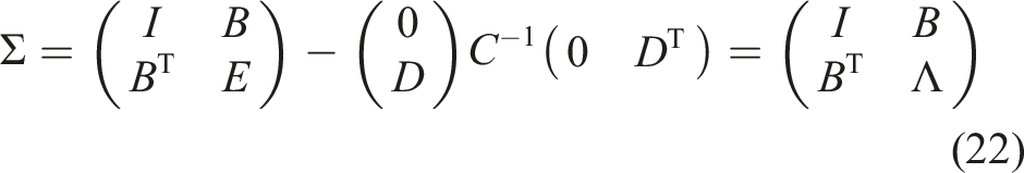
4.1.1. (M1) Direct Method 1
For the derivation of the first method, we substitute the suitably rearranged equations (10) and (12) into equation (11). For a better overview, Schur complements are denoted by Greek capital letters. Let Λ be the Schur complement of C in


Using block elimination and the above definitions, we obtain the solution


4.1.2. (M2) Direct Method 2
Another approach is substituting equations (11) and (12) into equation (10) of the block system. In this case one needs the Schur complement of Λ, instead of I, in

After rearranging, the procedure of solving the linear system of equations reads as


4.1.3. (M3) Semi-direct Method
The third method is semi-direct. The sets of indices

The first step (23) can be implemented using an iterative algorithm as the conjugate gradient method (Saad 2003). Each occurring product of the matrix Σ with a vector can be subdivided into the almost dense components, that is, multiplication with B and
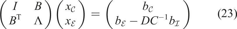
Note that within all three methods due to the block structure of the matrix C, its inverse C−1 only needs to be computed and saved once for each group of similar rectangles or triangles. In other words, if the coarse grid consists of M groups of similar elements and group i consists of m
i
similar elements for i ∈ {1, …, M}, we have
The same principle can be applied if a matrix is multiplied by C−1, which is important if the initial linear system is solved for multiple, Nrhs > 1, right-hand sides simultaneously leading to AX = B where
When comparing the direct methods (M1) and (M2) it is evident, that (M2) is more computationally demanding because, in contrast to (M1), it does not just involve the assembly of the matrix Λ but also its inversion. The semi-direct method (M3) has the advantage that besides C−1 no other storage consuming dense
4.2. Properties of the matrices
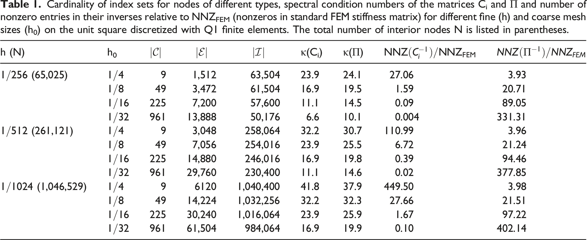
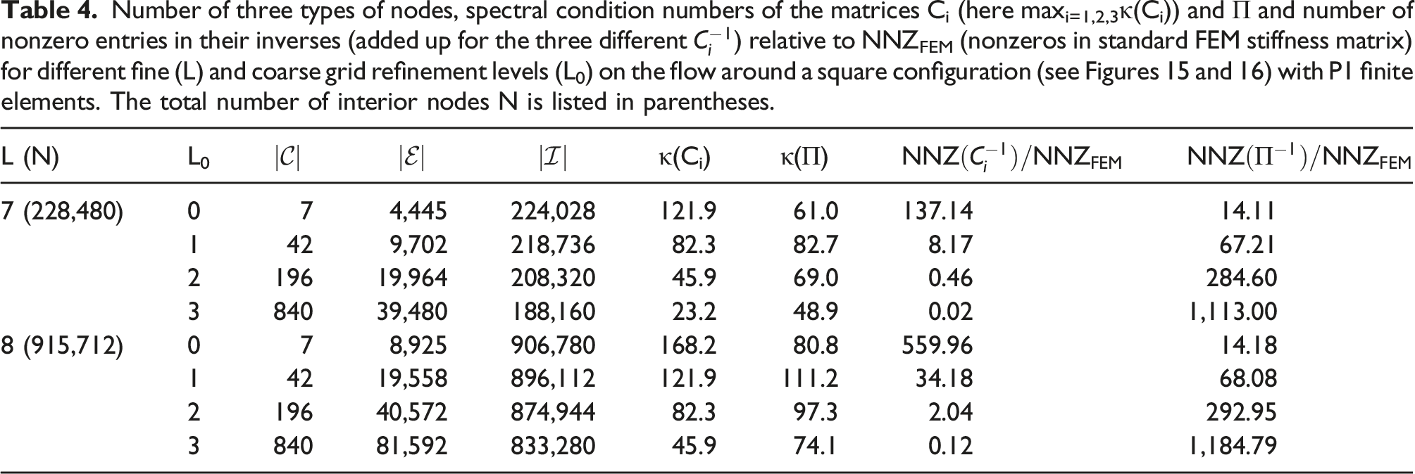
Cardinality of index sets for nodes of different types, spectral condition numbers of the matrices Ci and Π and number of nonzero entries in their inverses relative to NNZFEM (nonzeros in standard FEM stiffness matrix) for different fine (h) and coarse mesh sizes (h0) on the unit square discretized with Q1 finite elements. The total number of interior nodes N is listed in parentheses.
Obviously, the (M1) algorithm requires more storage than many standard approaches, especially because the dense inverse matrices
4.3. Estimation of complexity and storage requirement
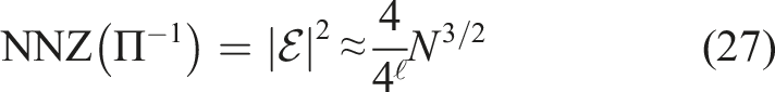
To determine an estimation of complexity and storage requirement, we first stick with the case of the unit square and Q1 finite elements and introduce the auxiliary variable ℓ that specifies by how many refinement levels the coarse grid width h0 differs from
We first estimate the storage cost for the dense matrix 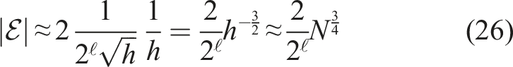
To obtain analogous results for 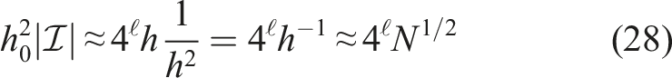

As a result, a matrix-vector multiplication with 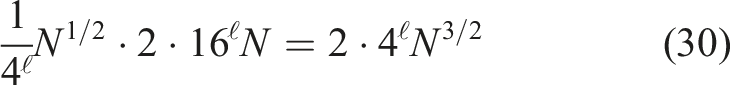
Note that the solution process of (M1) includes two applications of C−1.
To summarize, the total storage requirement of the relevant matrices of (M1) is
If the unit square is instead discretized with isosceles right triangles (with legs of length h) and linear (P1) finite elements are used, similar results can be derived. The basic difference to the Q1 case is that for the same values of h and h0 there are twice as many macro cells, fewer nodes in the interior and more nodes on the edges of the macro cells, namely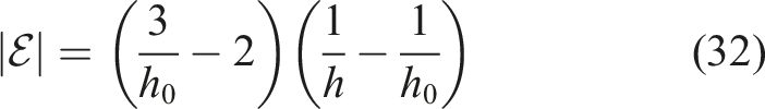
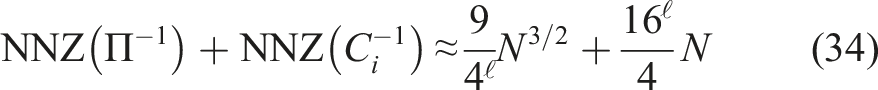
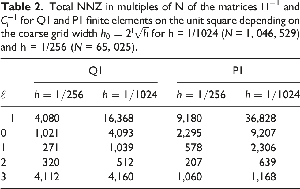
Total NNZ in multiples of N of the matrices Π−1 and
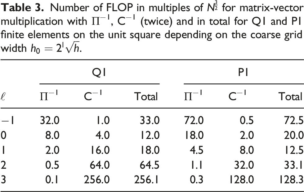
Number of FLOP in multiples of
5. Numerical results and comparison to standard FEM solvers on standard hardware
We now perform a numerical study to evaluate the new method (M1) in practice. In particular, we focus our attention to the question of whether we can exploit the computing power of the V100 and its Tensor Cores to achieve an advantage over a standard method, in this case a geometric finite element multigrid solver in double precision using the CSR format for matrices on the multicore AMD EPYC 7542 CPU. The geometric multigrid solver used in these benchmarks is a simple V-cycle multigrid which performs four smoothing steps of a Richardson iteration damped by the factor 0.3 as both a pre- and post-smoother on each multigrid level. The coarse mesh in the multigrid hierarchy consists only of one element, so all degrees of freedom on the coarse mesh are restrained by the Dirichlet boundary conditions and therefore no coarse grid solver is required. Because our benchmark problems do not contain anisotropies or other difficulties, this simple multigrid configuration turned out to be the most performant one in our tests as compared to configurations with more sophisticated smoothers such as ILU, SPAI or SOR, whose results we omit here because they are beyond the scope of this work. The associated software is the finite element software package FEAT3
1
(Ruelmann et al., 2021). Both hardware configurations are specified in the beginning of Section 2. We present numerical results for the unit square discretized using a uniform mesh of Q1 finite elements for the pairs of fine and coarse mesh sizes
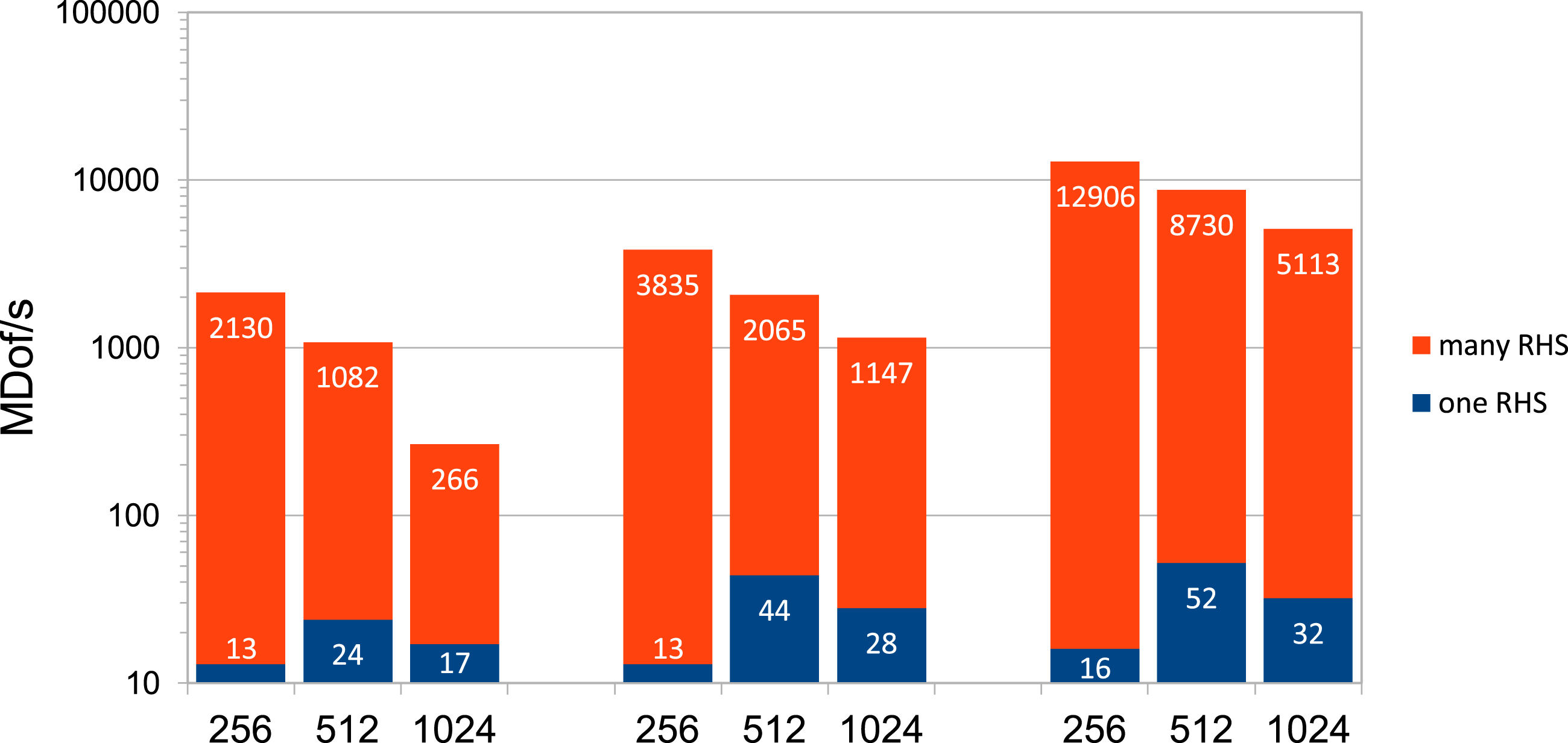
Figures 11 and 12 show the results of the new approach (M1) regarding GFLOP/s rates in Figure 11 and another measure, that is necessary to make the different methods comparable, that is, averaged number of million degrees of freedom solved per second (MDofs/s), in Figure 12, in double, single, and half precision and for one (Nrhs = 1) and many (Nrhs ≫ 1) right-hand sides, respectively. As expected, the case of solving Poisson’s equation on the same mesh for many right-hand sides simultaneously yields the highest performance. More precisely, we get an actual performance of 62,829 GFLOP/s or approximately 60 TFLOP/s in our study of (M1) with h = 1/1024, Nrhs ≫ 1 and in half precision on the V100 while (almost) no accuracy is lost due to the well-conditioned matrices. Furthermore, the outstanding performance depicted in Figure 11, especially in half precision, clearly indicates that the V100 is effectively used. According to the specification of the V100, the speed-up from single to half precision without Tensor Cores is a factor of 2 (with Tensor Cores 8). However, in this example it is 4.5 times faster in half precision due to Tensor Cores. GFLOP/s for (M1) with one and many RHS depending on h
−1
on the V100 GPU in DP, SP, and HP with Tensor Cores (left, middle, and right three columns, respectively). MDof/s (million degrees of freedom solved per second) for (M1) with one and many RHS depending on h−1 on the V100 GPU in DP, SP, and HP with Tensor Cores (left, middle, and right three columns, respectively).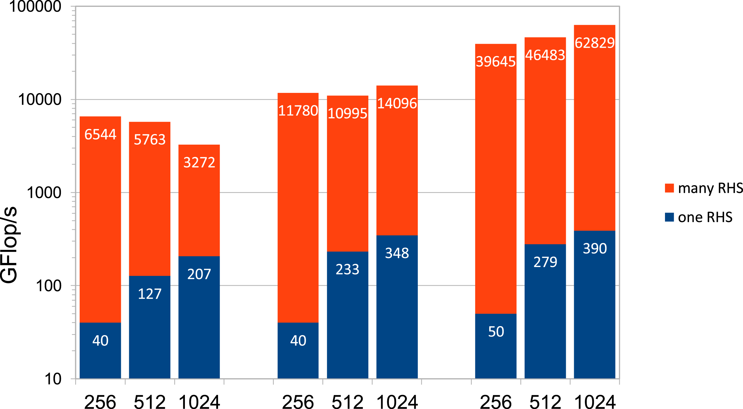
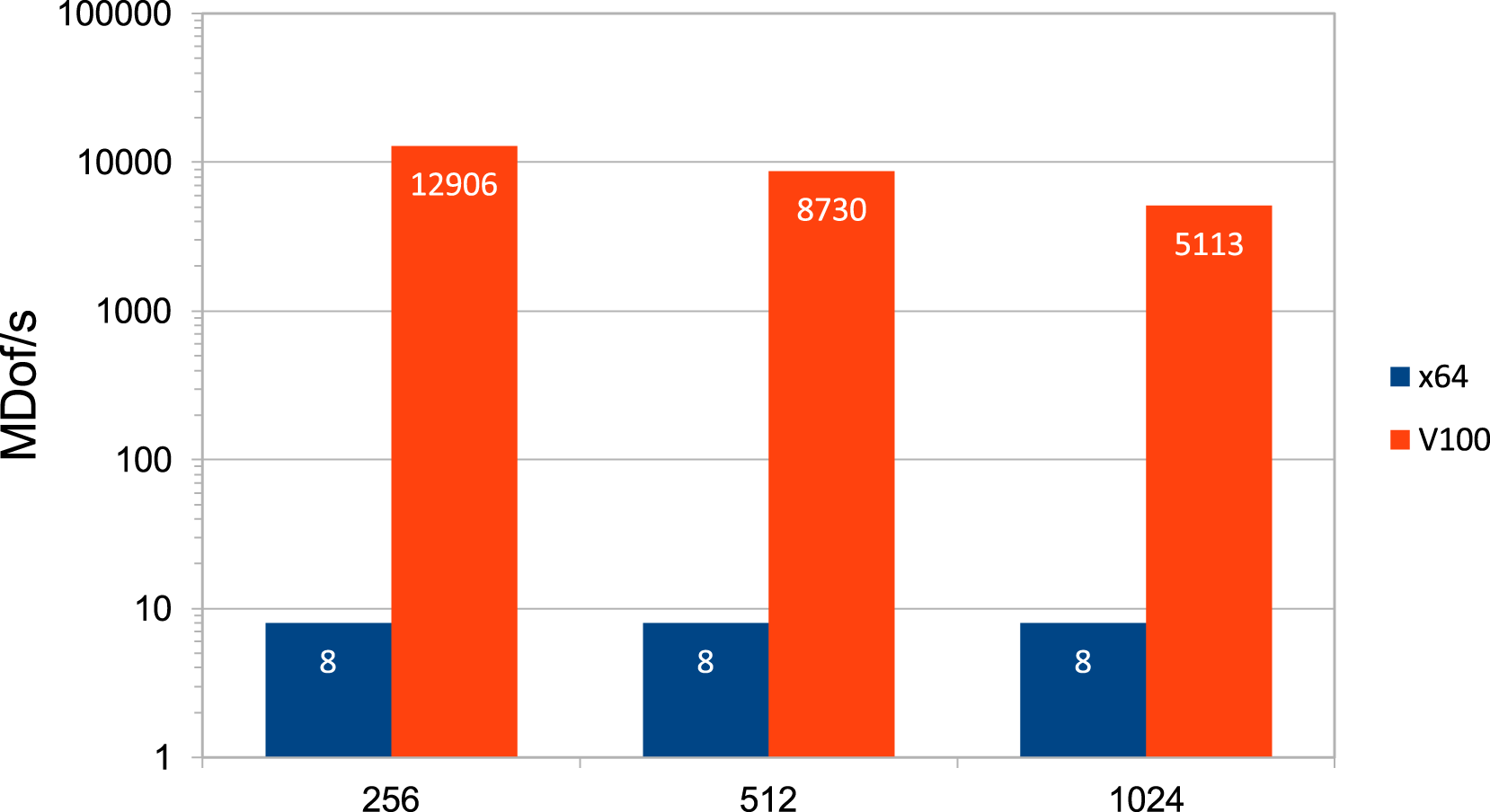
The observed GFLOP/s rates do not provide information about the efficiency of (M1) and do not enable a comparison to the standard method because we also need to take the complexity into account. As described in the previous section, we expect approximately MDof/s with a standard method (standard finite elements and multigrid in DP) on the AMD CPU (x64) for one and many RHS (left columns) and on the V100 for one RHS (right columns) depending on h−1. Comparison of MDof/s between standard method on the AMD CPU (left columns) and the direct method (M1) in HP with Tensor Cores on the V100 (right columns), both for many RHS, depending on h−1.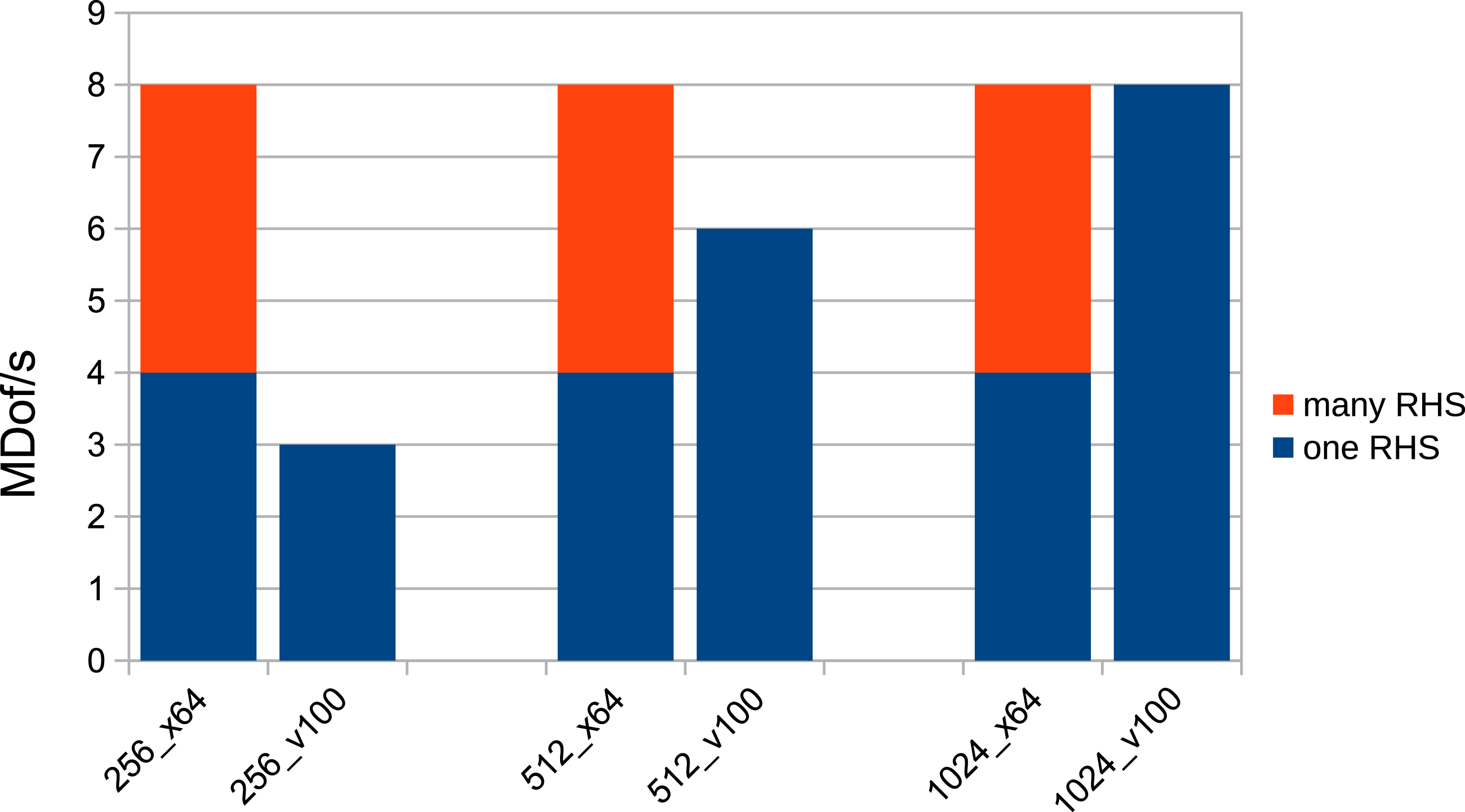
Regarding the scalability of the presented method, it can be said that for slightly higher problem sizes the performance might even further improve as the Tensor Cores can be better utilized. However, there is a limitation due to the high memory requirement of
5.1. Other meshes
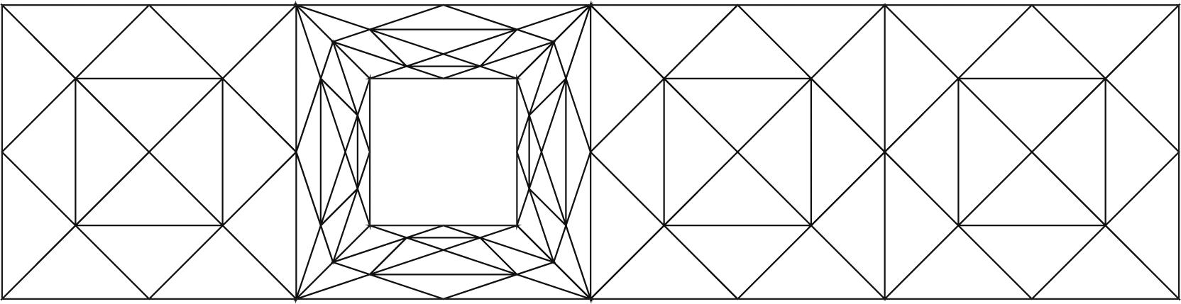
So far, we have only covered the simple case of the equidistantly refined unit square although the finite element multigrid method we use for comparative purposes is designed for arbitrary coarse grids, in particular partially unstructured coarse grids that are refined hierarchically. Nevertheless, the comparison of both methods is valid because the new approach (M1) can also be applied to partially unstructured and uniformly refined triangular coarse grids. Figures 15 and 16 show a (typical) flow around a square configuration as an example of a mesh we could also analyze with regard to (M1) with linear finite elements (P1) in the framework of this study. Coarsest mesh (level L = 0) of a flow around a square configuration on the domain Mesh shown in Figure 15 after one step of uniform refinement (level L = 1).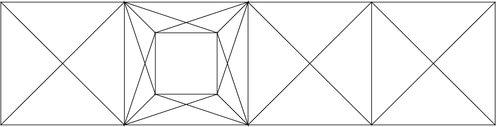
Number of three types of nodes, spectral condition numbers of the matrices Ci (here maxi=1,2,3κ(Ci)) and Π and number of nonzero entries in their inverses (added up for the three different
Another application of the method (M1) are meshes with high aspect ratios, such as anisotropic or skewed meshes. The convergence behavior of iterative multigrid methods gets significantly worse in this case, whereas the behavior of the direct method is hardly affected if such meshes are used.
5.2. Multiple right-hand sides
The presented direct method can also be used to accelerate time-dependent flow simulations modeled by the incompressible Navier–Stokes equations. To give an application example of this, we refer to operator-splitting methods, in particular discrete projection methods, that require the solution of a pressure Poisson problem in each time step. Only the right-hand sides of the linear systems change if the spatial mesh does not vary. A conjunction with currently examined time-simultaneous approaches (Dünnebacke et al., 2021) yields variants of the above-mentioned projection methods that allow for solving the pressure Poisson problems for all time steps simultaneously. That exactly corresponds to the case of a system AX = B with a constant stiffness matrix A and a matrix of solutions X and right-hand-sides B with Nrhs ≫ 1 columns, in which the highest performance is reached in our tests.
6. Summary and outlook
The purpose of this work was the development and numerical study of a new hardware-oriented algorithm based on knowledge of modern special hardware. As a result, we are able to combine high numerical efficiency with the computational performance of the V100 GPU and its Tensor Cores.
Clearly, our studies are preliminary and only cover the case of Poisson’s equation so far. However, this problem represents a central component of many numerical methods for flow simulations using the time-dependent incompressible Navier–Stokes equations. The additional use of parallelism in such basic components of advanced simulation software for applications in numerical continuum mechanics can reduce the computing time by orders of magnitude
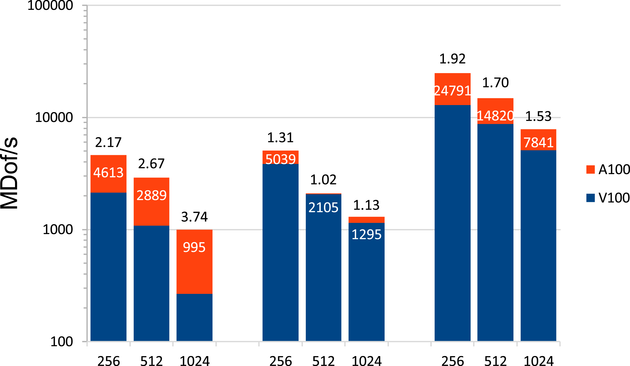
Of course, further research needs to be carried out on prehandling in 3D, other differential operators and finite element spaces, as well as on semi-direct variants of the Schur complement approach, such as the method (M3) we also derived. The list of interesting open problems also includes analysis of the new method on other current GPUs. The presented studies, showing the possible gain in efficiency in mathematical simulation tools (especially in numerical continuum mechanics), prove to be even more important considering that the supercomputer JUWELS at Forschungszentrum Jülich, Germany ranked eighth in the current TOP500 list (June 2021) as the fastest European computer system (TOP500, 2021). Its booster module is based on the NVIDIA Ampere A100 Tensor Core GPU, the successor model of the V100. The A100 GPU promises more than 300 TFLOP/s with Tensor Cores in half precision (NVIDIA 2021) which becomes (nearly fully) exploitable by means of prehandling techniques as the results of preliminary tests presented in Figures 17 and 18 show. The results shown inside the columns were obtained with the A100 and can be compared with the values shown in Figures 11 and 12. Indeed, we obtain a further acceleration by approximately 50%. GFLOP/s for (M1) with many RHS depending on h−1 on the V100 and the A100 GPU in DP, SP, and HP with Tensor Cores (left, middle, and right three columns, respectively) with speed-up indicated above the columns. MDof/s for (M1) with many RHS depending on h−1 on the V100 and the A100 GPU in DP, SP, and HP with Tensor Cores (left, middle, and right three columns, respectively) with speed-up indicated above the columns.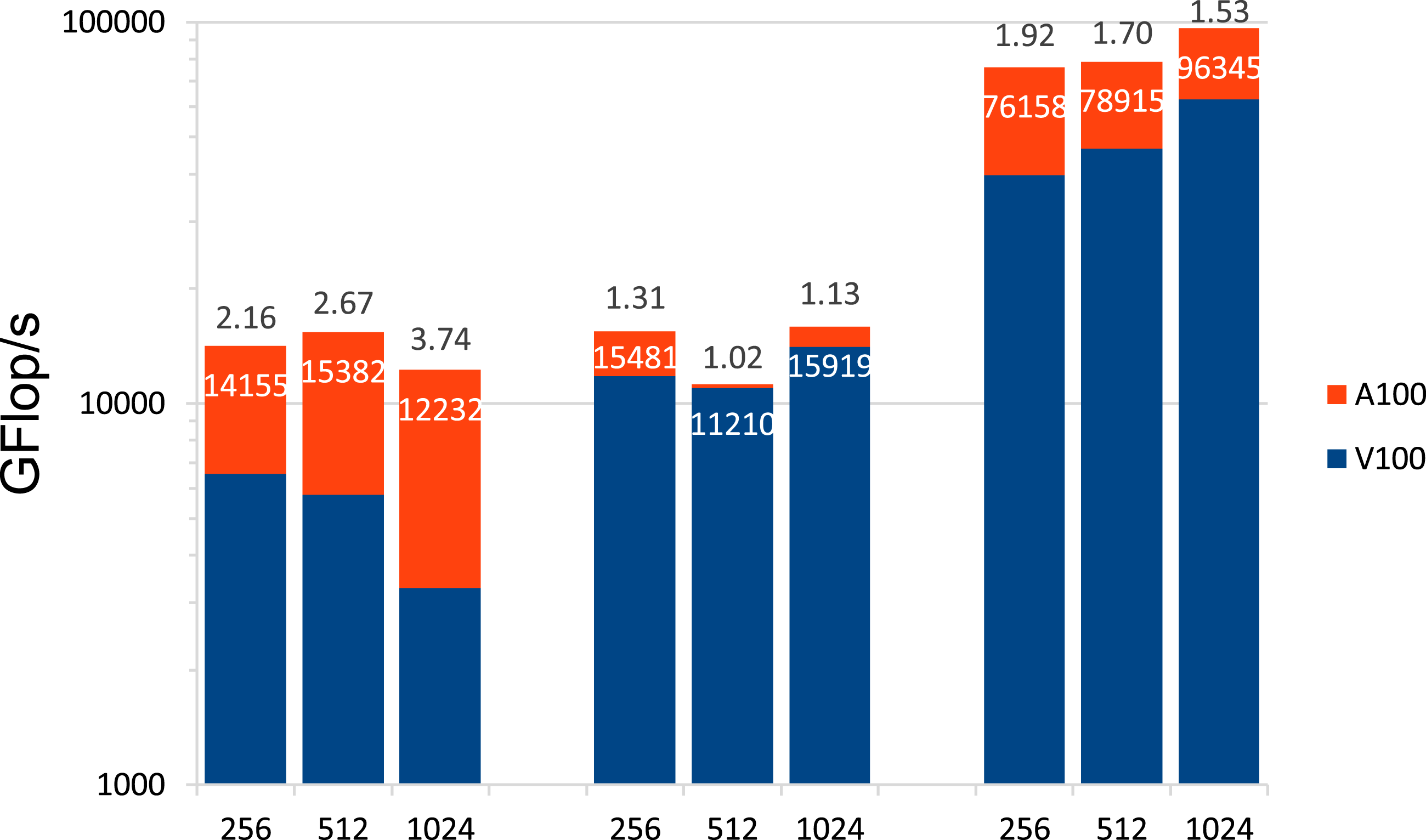
Footnotes
Acknowledgements
All comparative results presented in Section 5 have been created using the FEM software package FEAT3 2 , whereby calculations have been carried out on the LiDO3 3 cluster at TU Dortmund University. We gratefully acknowledge the extensive programming work of Heiko Poelstra during the preparation of this study.
Declaration of conflicting interests
The author(s) declared no potential conflicts of interest with respect to the research, authorship, and/or publication of this article.
Funding
The author(s) received no financial support for the research, authorship, and/or publication of this article.
Notes
Author biographies
Dustin Ruda completed his master’s degree in Mathematics at TU Dortmund University in 2020, where he has since been working as a PhD student at the Chair of Applied Mathematics and Numerics. His research interests include the adaptation of finite element approaches for elliptic problems and construction and analysis of solution methods that allow the use of fast low precision hardware.
Stefan Turek obtained his PhD in Mathematics from the University of Heidelberg and has been regular professor for Applied Mathematics and Numerics at TU Dortmund University since 1999. He has published more than 200 papers/conference contributions in the field of numerics for PDEs and finite element methods, multigrid solvers, computational fluid dynamics, and high performance computing. Besides, he is strongly involved in developing basic FEM software (FEAT) and the open-source CFD package FEATFLOW (www.featflow.de). Recently, the main research topics of his group of PhD students, postdocs, and collaborators is computational fluid dynamics and the development and realization of simulation techniques and massively parallel HPC software including hardware-oriented numerics and machine learning on special hardware (GPU, TPU) for technical simulations in continuum mechanics and life science.
Dirk Ribbrock studied Computer Science at TU Dortmund University and finished his diploma thesis in 2010. Since then, he has been working as a research assistant at the Chair of Applied Mathematics and Numerics. His research interests are hardware-oriented numerics and parallelization of numerical applications, especially via GPU.
Peter Zajac finished his mathematics diploma thesis in 2011 at TU Dortmund University and is employed at the faculty of mathematics of TU Dortmund since then, where he is one of the main educational staff responsible for the teaching of programming languages. He is the lead developer of the Finite Element Analysis Toolbox 3 (FEAT3) and is responsible for its continuous kernel development as well as for the introduction and support of new and existing programmers and users to this software. His main research fields are the development of geometric multigrid methods for large parallel clusters as well as the construction and analysis of finite element spaces.