Sage Journals: Discover world-class research

Abstract

We improved the quality and reduced the time to produce machine learned models for use in small molecule antiviral design. Our globally asynchronous multi-level parallel training approach strong scales to all of Sierra with up to 97.7% efficiency. We trained a novel, character-based Wasserstein autoencoder that produces a higher quality model trained on 1.613 billion compounds in 23 minutes while the previous state of the art takes a day on 1 million compounds. Reducing training time from a day to minutes shifts the model creation bottleneck from computer job turnaround time to human innovation time. Our implementation achieves 318 PFLOPs for 17.1% of half-precision peak. We will incorporate this model into our molecular design loop enabling the generation of more diverse compounds; searching for novel, candidate antiviral drugs improves and reduces the time to synthesize compounds to be tested in the lab.

Keywords

COVID 19 machine learning scalable performance generative models drug design

1. Justification

Using scalable deep learning tools, we produce an accurate generative model with low reconstruction error, improve training time from a day to 23 minutes, and increase search efficiency for COVID drug discovery. Our model achieves 17.1% of half-precision peak and near perfect strong scaling to all of Sierra.

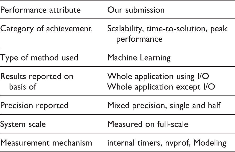
2. Performance attributes

Performance attribute	Our submission
Category of achievement	Scalability, time-to-solution, peak performance
Type of method used	Machine Learning
Results reported on basis of	Whole application using I/O Whole application except I/O
Precision reported	Mixed precision, single and half
System scale	Measured on full-scale
Measurement mechanism	internal timers, nvprof, Modeling

3. Overview of the problem

COVID-19 is the second worst pandemic in US history, with over 216,000 deaths and 7.8 million cases as of October 8, 2020. The only pandemic with more US fatalities was the Spanish Flu pandemic, which killed around 675,000 Americans in 1918–1919 (Centers for Disease Control and Prevention, 2020). Historically, the death toll of the 1957 flu pandemic was curbed by Maurice Hilleman, whose work at the Walter Reed Army Institute of Research led to the quick development of a vaccine in the summer of 1957 (Zeldovich, 2020). Like then, the world is now racing to discover therapeutics to stifle the spread of SARS-CoV-2 and curb its death toll.

A significant amount of attention has been given to the development of vaccines that can prevent the manifestation of COVID-19. However, there are other therapeutic options like therapeutic antibodies and small molecule antivirals. Ideally all three therapies would be developed simultaneously and each requires a distinct development path. It is painstakingly slow to develop a new therapeutic that is both safe and effective, so we have focused our efforts on discovering and designing candidates for small molecule antivirals.

The discovery phase of drug development involves three tasks: hit identification, where chemical compounds with promising activity are identified; lead generation, where hit compounds are improved; and lead optimization, where lead compounds are optimized to become more drug-like with beneficial pharmacological effects. These tasks are pursued with the basic strategies of structure-based drug design (SBDD) and ligand-based drug design (LBDD). Both approaches involve screening large datasets of small molecule compounds and are limited by the type of input that is needed. SBDD is used when a 3-dimensional structure is available for the protein target and physics-based algorithms can be applied to calculate the binding energy between a small molecule and a protein target. These physics-based methods, such as molecular docking and molecular dynamics, are extremely computationally expensive and can be slow, precluding their use as a screening method on large chemical libraries. However, large chemical libraries can be screened earlier, starting with hit identification. There has also been some success applying machine learning (ML) to predict small molecule binding to the protein target (Zhu et al., 2020). LBDD is used when no structural information is available, and initial hit identification is frequently acquired experimentally by running high-throughput biochemical assays. Then, quantitative structure activity relationship (QSAR) models are trained on the experimental data and deployed for lead generation to optimize a biological activity. This approach suffers from the need to have a set of active compounds to train these models.

Whether using LBDD or SBDD approaches, the less obvious limitation is the lack of diversity and robustness in the chemical compounds used for lead generation and optimization. Once hits are identified and design criteria are known, new molecules need to be suggested and evaluated against the design criteria. The new compounds must be synthesizable and have acceptable drug-like properties, such as permeability and minimal toxicity. In principle, ML can be used to guide the search of chemical space where new compounds are similar to promising hits but different enough to improve one or more design criteria. Figure 1 shows the concept of a generative molecular design loop where candidate drug-like molecules are proposed and evaluated with LBDD and SBDD methods, searching through a latent space (green) until converging on a set of candidate molecules that meet the required design criteria.

Figure 1.

Generative design loop overview. Compounds are evaluated against drug design criteria to optimize for properties, such as minimal toxicity. After each iteration of compound evaluation, compounds in the latent space (green) of the generative model are perturbed to move closer to meeting the design objectives. The molecules are decoded from the latent space to generate new molecules for evaluation in the next design iteration.

There do exist large chemical databases like GDB-17, which contains 166.4 billion molecules that are claimed to be synthesizable and stable (Reymond, 2015). However, it is currently not possible to search this exceptionally large chemical space without faster physics-based scoring methods or better ML models. Chemical suppliers, such as Enamine, now offer a list of 1.36 billion drug-like compounds. This large list of purchasable compounds opens the door to train higher-quality generative neural network models but also introduces computational challenges. The best models today take at least a day to train on even a million compounds, and frequently several prototyping iterations are needed to find a good model architecture. While it is possible to train on a subset of the data, the model can become biased toward molecules that are already promising, leaving out valid regions in the chemical space. With all this considered, training on large datasets with a reasonable training time is critical to maximize the odds of designing the next antiviral drug.

4. Current state of the art

4.1. Biology/chemistry

Deep learning has the flexibility to be applied in a number of areas of drug design from 3D convolutional neural networks on structural data to graph-based neural networks trained on identified hits, to generative adversarial trained models on specific properties.

The traditional approach to chemical exploration is a fragment based search which uses a starting fragment to seed a combinatorial search through chemical space using successive modifications to the starting fragment (Price et al., 2017). Fragment based search depends on human medicinal chemistry expertise and intuition. Alternatively, deep learning generative models implemented in the form of variational autoencoders (VAE) (Kingma and Welling, 2013; Rezende et al., 2014) were recently introduced as a modeling tool for encoding a virtual chemical library in continuous latent space (Blaschke et al., 2018; Gómez-Bombarelli et al., 2018; Sanchez-Lengeling and Aspuru-Guzik, 2018). The latent space representation creates a nearly infinite source of new molecules to evaluate and are derived from a learned chemical representation that captures the desired chemical properties provided from example compounds. The character VAE (cVAE) biases the compound search space based on a corpus of training data. Trainable desired properties include strong binding potential to a protein target and efficient synthesis of new chemical compounds for experimental testing. However, the challenge for VAE models is in generating syntactically correct and semantically meaningful molecules from the linear representation of a molecular input as a simplified molecular-input line-entry system (SMILES) string. Current methods to improve the accuracy of the representation include (1) the Junction Tree VAE (JT-VAE), which generates a tree of molecular fragments connected with a molecular graph (Jin et al., 2018), (2) constraints in the character VAE decoder step (Winter et al., 2019a) to generate real molecular structures, and (3) introduce adversarial training (Maziarka et al., 2020). Other methods can generate realistic molecular structures using recurrent neural networks and the long short-term memory algorithm for generative modeling (Gupta et al., 2017) but do not maintain the fixed sized latent vector that can be used for directed optimization. More recently, the latent space of generative models has been used to support iterative search of the latent space (Hinkson et al., 2020; Winter et al., 2019b); predicted properties for a newly generated molecule are taken from a machine learning model and used to guide sampling from the design space (Brookes et al., 2019).

A possible new autoencoder to apply to molecular design is the Wasserstein autoencoder (WAE) (Tolstikhin et al., 2017), which incorporates adversarial training in the latent space and has shown improved model accuracy in computer vision applications.

4.2. Large scale machine learning

Within the field of machine learning (ML) there are a few key concepts that are worth stating to ensure consistent terminology. Deep Neural Network (DNN) models consists of a network architecture and associated set of connection weights that are the learned parameters. To train these parameters the data set is processed in chunks of data called mini-batches. After each mini-batch of data is processed, a step is done in the stochastic gradient descent (SGD) algorithm, optimizing the weight parameters. Processing the entire data set once is a training epoch, and the training continues through multiple epochs until a target objective function is reached. In this work we used the Livermore Big Artificial Neural Network (LBANN) toolkit (Van Essen et al., 2015), a scalable framework for the training and inference of DNN models on leadership-class HPC systems.

Traditional approaches to large-scale training of DNNs are data and model parallelism (Coates et al., 2013; Dean et al., 2012; Goyal et al., 2017; Iandola et al., 2015; Keskar et al., 2017; Recht et al., 2011). In model parallelism, the parameters (i.e. weights) of a single model are distributed across the computing elements. In data parallelism, each mini-batch of input data is partitioned across the computing elements and processed concurrently, while the model parameters (weights) are replicated. Updates to the model are then aggregated across all samples, and distributed to each processing element. These two broad approaches are typically discussed within the context of training a single model to some level of convergence. However, these strategies tend to be limited by the performance overhead of inter-process (collective) communication, and harmful effects on learning behavior (Keskar et al., 2017).

Data parallelism relies on large mini-batches, known as large-batch training, to increase the computational work per process, it is inherently limited because it negatively impacts the quality of learning. Several research efforts have been dedicated to addressing this problem, most prominent of which is linear learning rate scaling and its variants (Akiba et al., 2017; Goyal et al., 2017; You et al., 2018, 2019). Even so, these approaches have only been shown to perform well on computer vision problems. Our initial exploration into scaling up the mini-batch size showed minor improvement with linear rate scaling.

Scientific simulations and experimental data are drawing attention from large-scale machine researchers. Prominent recent works that leverage HPC systems at scale are: exascale deep learning for climate analytics (Kurth et al., 2018), $C o s m o F l o w$ that used deep learning to learn the universe at scale (Mathuriya et al., 2018) and a complex generative surrogate model trained on millions of high-energy physics multivariate data (Jacobs et al., 2019). While there have been applications of machine learning techniques in drug design space, we are not aware of training of such models at a billion drug compound scale.

5. Innovations realized

5.1. Model design

5.1.1. Model architecture

Our scalable machine learning approach enables data scientists to train ML models quickly on large data sets. By reducing training times from multiple days to under an hour, we allow for rapid prototyping and experimentation, resulting in less time needed to develop a higher-quality model.

Using a newly designed character WAE (cWAE), we prototyped, explored, and trained a high-quality model on 1.613 billion compounds in less than a week of developer time. This model architecture has never previously been applied to molecular design, and our initial results are promising such that the model will be incorporated into the molecular design loop. In addition, we also explored the performance of the cWAE model at various scales, both in terms of compute resources and data set size. This cWAE model completely out performed an extensively trained cVAE built out of gated recurrent units (GRU) (Cho et al., 2014).

Our cWAE model (see Figure 2 and Table 1) is made up of three components: (1) an encoder converts a sequence of embedding vectors into a vector in a latent space, (2) a decoder reconstructs the original sequence from a latent space vector, and (3) a discriminator attempts to classify the probability distribution that generated a given latent space vector. A molecule’s SMILES string is first truncated or padded to a sequence length of 100 and projected into an embedding space. The encoder applies a single-layer GRU to the embedding sequence and a fully-connected layer to the final state to produce a latent space vector. The decoder concatenates the latent space vector with the embedding sequence and applies a three-layer GRU and fully-connected layer to recover the original sequence. The discriminator is a simple multi-layer perceptron that attempts to classify whether a latent space vector (concatenated with the embedding sequence) was generated by the encoder or drawn from a unit Gaussian distribution. The encoder and discriminator are trained adversarially so that the encoder learns to generate a Gaussian distribution of latent space vectors. Notably, the bulk of the computation occurs in the GRUs in the encoder and decoder.

Figure 2.

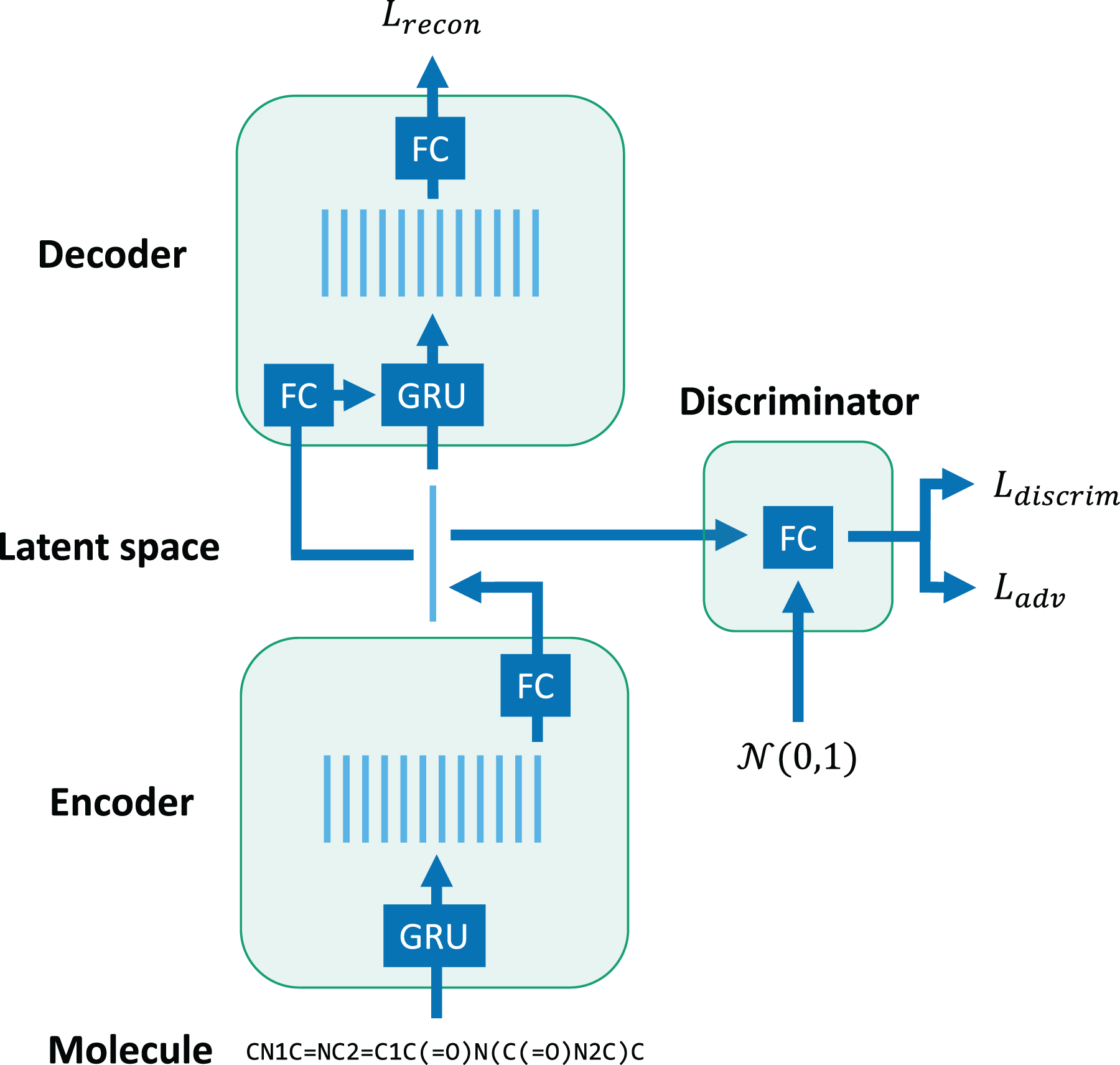
High-level design of character Wasserstein autoencoder (cWAE) model. The network consists of GRUs and fully connected (FC) layers.

Table 1.

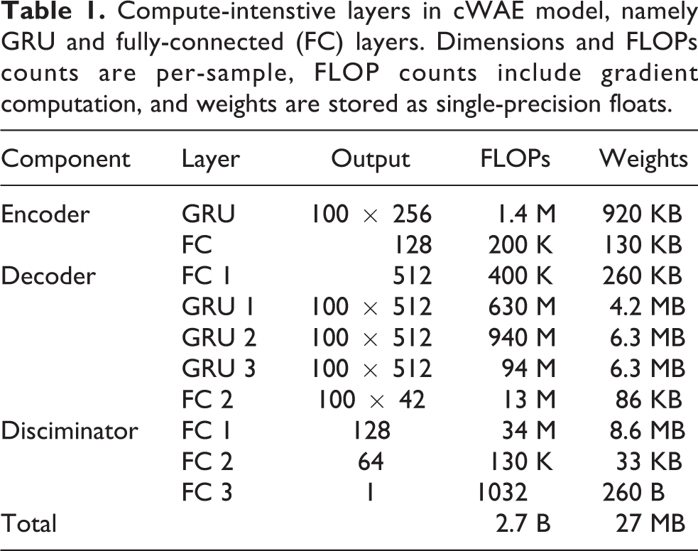
Compute-intenstive layers in cWAE model, namely GRU and fully-connected (FC) layers. Dimensions and FLOPs counts are per-sample, FLOP counts include gradient computation, and weights are stored as single-precision floats.

Component	Layer	Output	FLOPs	Weights
Encoder	GRU	$100 \times 256$	1.4 M	920 KB
	FC	$128$	200 K	130 KB
Decoder	FC 1	$512$	400 K	260 KB
	GRU 1	$100 \times 512$	630 M	4.2 MB
	GRU 2	$100 \times 512$	940 M	6.3 MB
	GRU 3	$100 \times 512$	94 M	6.3 MB
	FC 2	$100 \times 42$	13 M	86 KB
Disciminator	FC 1	$128$	34 M	8.6 MB
	FC 2	$64$	130 K	33 KB
	FC 3	1	1032	260 B
Total			2.7 B	27 MB

5.1.2. Model evaluation

We trained our model on nearly an order of magnitude more chemical compounds than any other work reported in the literature. A recent review of generative models (Elton et al., 2019) reports the largest previous training set to be the ZINC library with 192.8 million molecules. The authors note that they actually only trained on a subset of the total number of molecules (Skalic et al., 2019), so our data set size may be even more than an order of magnitude larger. For our study, data was combined from three sources: (1) a recent collection from the Enamine REAL database (Enamine, 2020) downloaded in the first quarter of 2020, (2) a non-overlapping list of historical Enamine compounds downloaded in the first quarter of 2018, and (3) 1 million additional purchasable compounds screened for SARS-CoV-2 main protease (Mpro) inhibition activity for a total of 1.613 billion compounds.

Model accuracy was compared for three different generative models: 1) cWAE trained on the general Enamine library and predicted main protease (Mpro) inhibitors, 2) cWAE trained on just the 1 M predicted Mpro inhibitors and 3) our previous modeling approach using the JT-VAE and trained on just the Mpro inhibitors. With the current implementation, it was not technically feasible to train the JT-VAE on the Enamine library because of the large size of the data set. Two held out test sets were used to evaluate model accuracy: (1) ten thousand compounds drawn at random from the combined Enamine and Mpro inhibitor libraries and (2) ten thousand compounds randomly drawn from the Mpro inhibitor set only.

The model accuracy results are shown in Table 2 and show important improvements in the newly trained models. One key metric, compound reconstruction rate, is the fraction of compounds for which encoding followed by decoding reconstructs the original molecule. Another is the average Tanimoto distance between the encoded and decoded SMILES strings, computed with the RDKit package (RDKit, 2020). The goals of model training are to minimize these distances, and to create a latent space representation in which small perturbations of latent vectors result in small changes to the decoded structures. These metrics are key to the molecular design application, wherein we navigate in the latent space to optimize desired molecular properties. For the Enamine trained model and testing on a combination of Enamine and Mpro inhibitor molecules, reconstruction accuracy is exceptionally high with a compound reconstruction rate of 90.14% and an average Tanimoto distance of 0.08. Validity rate measures the fraction of decoded SMILES strings that are syntactically correct, and a higher percentage is needed to avoid inefficient search through invalid compound proposals. As expected, the models trained exclusively on the Mpro inhibitor data set are more accurate at reconstructing the Mpro inhibitor test molecules, however, they will fail to act as generalized molecule proposal models given their limited training.

Table 2.

Summary of model accuracy. Metrics include percent of valid decoded SMILES strings (Percent Valid), Compound Reconstruction Rate and Average Tanimoto Distance between the encoded and decoded molecule (Average Tanimoto Distance, lower is better).

Model	Train Size	Test Size	Percent Valid	Compound Reconstruction Rate	Average Tanimoto Distance
JT-VAE (state of the art)	1 M Mpro	10 K Mpro	100	1.63	0.553
cWAE	1 M Mpro	10 K Mpro	85.41	83.27	0.146
cWAE	1613 M Combo	10 K Mpro	42.45	33.03	0.601
cWAE	1613 M Combo	10 K Combo	92.70	90.14	0.080

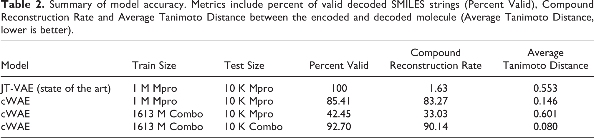
Even for the Mpro reconstruction, the larger trained model shows a higher compound reconstruction rate (33.03%) than the baseline JT-VAE (1.63%), although with a lower validity rate of 42.45% versus 100%. These results suggest that we can build two different cWAE models, and both have distinct accuracy advantages over the JT-VAE trained model. The cWAE model trained on the largest training set to date, is exceptionally accurate for purchasable compounds from Enamine. The cWAE trained on the smaller Mpro data shows reduced accuracy overall but is more accurate than the JT-VAE on the Mpro inhibitor test molecules with a compound reconstruction rate of 83.27% and a relatively high validity rate (85.41%). A molecular design loop has the potential to use both of these improved models, using the Enamine trained model to propose a diverse range of makeable compounds to test and can compliment the Mpro model trained on examples identified as promising in subsequent iterations of the design loop.

5.2. Performance optimizations

5.2.1. Single-GPU tuning

We focused our optimization efforts on the matrix multiplications within the GRU that dominate the runtime of the cWAE model. Our initial testing used single-precision computation, and we found that it was compute-bound for even small mini-batches. This motivated us to investigate computation at lower precision since V100 GPUs can achieve 8x higher half-precision performance than single-precision performance. This peak performance requires using tensor cores, which perform computation at half-precision. We found that training GRUs with half-precision computation and data was unstable and would diverge on larger data sets ( $> 1 M$ samples). Using half-precision computation accumulated into single-precision data was more stable allowing us to get a 2.0x speedup from the tensor cores.

Profiling revealed that our next bottleneck was the latency cost of launching many small kernels. To reduce this cost, we leveraged CUDA graphs to amortize the overhead of multiple kernel launches into one graph launch. We note that support for CUDA graphs was first introduced in cuDNN 8, which also introduced a new RNN API. Upgrading to the new RNN API imposed performance penalties for certain problem sizes, but they were offset by the performance gains from CUDA graphs. We also observed that computing a graph is more expensive than running kernels directly, so we cached the graphs to reuse them as much as possible.

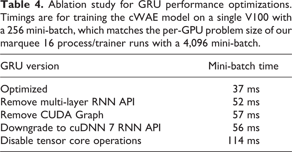
Our final optimization was to fuse stacked GRU layers into a single cuDNN API call, which enabled internal performance optimizations in cuDNN. The final result of these optimizations was a 3.0x improvement in model training time, relative to the single-precision implementation. Table 4 shows the effect of each of these optimizations.

5.2.2. Data ingestion improvements

Fast data ingestion is important for good performance at scale. LBANN already implemented a global parallel data store (Jacobs et al., 2019) that uses system DRAM. We improved LBANN’s SMILES data reader to take full advantage of the data store. Sierra has over a petabyte of collective DRAM, which is more than enough capacity for our data set.

5.2.3. Removing global synchronization

LBANN scales to thousands of nodes, using the “Let a Thousand Flowers Bloom” (LTFB) approach, a distributed variation on population-based training (Jacobs et al., 2017; Jaderberg et al., 2017). By grouping compute nodes into trainers, each of which trains a model independently on its own subset of the training set. At regular intervals, the trainers pair up, exchange models, and evaluate on a held-out data set. The trainers then continue training the model that performs better. Prior to our work LBANN had rank 0 distribute all of the partners for this exchange. This was done at a global synchronization point.

Globally synchronous operations hurt run time because their performance is limited by the slowest process in the parallel application. Node performance is stochastic due to system noise (Petrini et al., 2003; Tabe et al., 1995), and becomes especially problematic at scale. Furthermore, compute-intensive applications on GPUs draw a substantial amount of power, so idling all the GPUs at once during a synchronization can cause sudden swings in power load.

To resolve the power issues observed when running LBANN and improve scalability, it was rearchitected to avoid all global synchronizations during training. Synchronizations during LTFB exchanges were removed by having each trainer compute partner assignments independently based on a shared random seed. Computation of global statistics for metrics and timings was also disabled and replaced with offline post-processing.

6. How performance was measured

6.1. Applications used to measure performance

We performed training using the Livermore Big Artificial Neural Network Toolkit (LBANN) (Van Essen et al., 2015), version 0.102.0-dev. LBANN was built with the following stack:

Hydrogen 1.5.0-dev (Maruyama et al., 2020), a GPU-enabled fork of Elemental (Poulson et al., 2013): Performed distributed linear algebra.

Aluminum 0.6-dev (Dryden et al., 2018): Performed asynchronous GPU communication.

Conduit 0.5.1 (Larsen et al., 2018): Used to implement distributed in-memory data store.

Merlin 1.7.4 (Peterson et al., 2019): Generated experiments and managed job submissions.

We used a 1.613 billion molecule training set and a 2.01 million molecule test set. All of our reported results used a mini-batch size of 4,096. In small-scale tests, training with larger mini-batch sizes caused learning to diverge, even with the standard techniques of learning rate scaling and linear warmup (Goyal et al., 2017; You et al., 2019). Smaller mini-batches achieved significantly worse time to solution.

6.2. Data collection

All of our experiments used a 4,096 mini-batch size and learning rate of 0.0024. We ran tests with 8 or 16 GPUs per trainer. One LTFB exchange occurred per epoch. Tests were scaled from 64 nodes to 2,048 nodes by powers of 2 and we ran our largest test at 4,160 nodes. The number of trainers in each experiments can be found by $(n o d e s * 4) / (G P U s p e r t r a i n e r)$ . Our 1.613 billion samples were divided evenly among trainers. For 64 nodes with 16 GPUs per trainer each trainer had 99,803,756 samples, and this became 767,721 samples per trainer at 4,160 nodes with 8 GPUs per trainer.

LBANN reported timings (data ingestion times, epoch times, mini-batch times) and metrics (reconstruction loss on training, tournament, and test data sets). We measured both full application time to trained model and the performance of the training portion of the code. Livermore Computing provided power measurements using wall plates in the machine room that directs power to Sierra.

FLOP counts were estimated analytically based on the matrix dimensions in the GRUs and fully-connected layers. These FLOP estimates were validated by comparing against empirical measurements from nvprof, which had a discrepancy less than 4%. We note that nvprof does not report accurate FLOP counts unless CUDA graphs are disabled. Nearly all the FLOPs were computed at half-precision and accumulated into single-precision data. For simplicity we do not distinguish between half-precision and single-precision FLOPs in our performance analysis.

Power measurements came from facility data collection. Measurements are reported every second in watts for 10 measurement devices. These cover five of the six compute rows of Sierra.

6.3. Measuring model quality

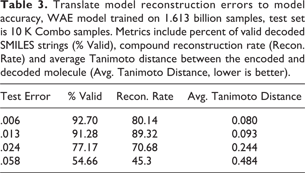
Understanding when a model has been sufficiently trained is a perennial problem for domain scientists. Fortunately, there are several clear metrics for this application: Percent Valid, compound reconstruction rate, and Average Tanimoto Distance. Table 3 helps translate the abstract test reconstruction error into well quantified metrics. According to our domain scientists a model with an error of $0.024$ or less is sufficient for the current reconstruction task.

Table 3.

Translate model reconstruction errors to model accuracy, WAE model trained on 1.613 billion samples, test set is 10 K Combo samples. Metrics include percent of valid decoded SMILES strings (% Valid), compound reconstruction rate (Recon. Rate) and average Tanimoto distance between the encoded and decoded molecule (Avg. Tanimoto Distance, lower is better).

Test Error	% Valid	Recon. Rate	Avg. Tanimoto Distance
.006	92.70	80.14	0.080
.013	91.28	89.32	0.093
.024	77.17	70.68	0.244
.058	54.66	45.3	0.484

7. System and environment where performance was measured

We ran our tests on the 4,320 node Sierra supercomputer at LLNL (Vazhkudai et al., 2018).

7.1. Hardware environment

Each Sierra node contains two 22-core IBM Power9 CPUs and four Nvidia V100 GPUs. A GPU has 16 GB local memory and two GPUs are connected to a CPU with 75 GB/s NVLink interconnects. A GPU is capable of 112 half-precision TFLOPS using tensor cores, so the system peak performance is 1.9 EFLOPS. Each node has a dual-port EDR InfiniBand NIC, with each port providing 12.5 GB/s bi-directional bandwidth. See Figure 3 for a detailed view of the node architecture.

Figure 3.

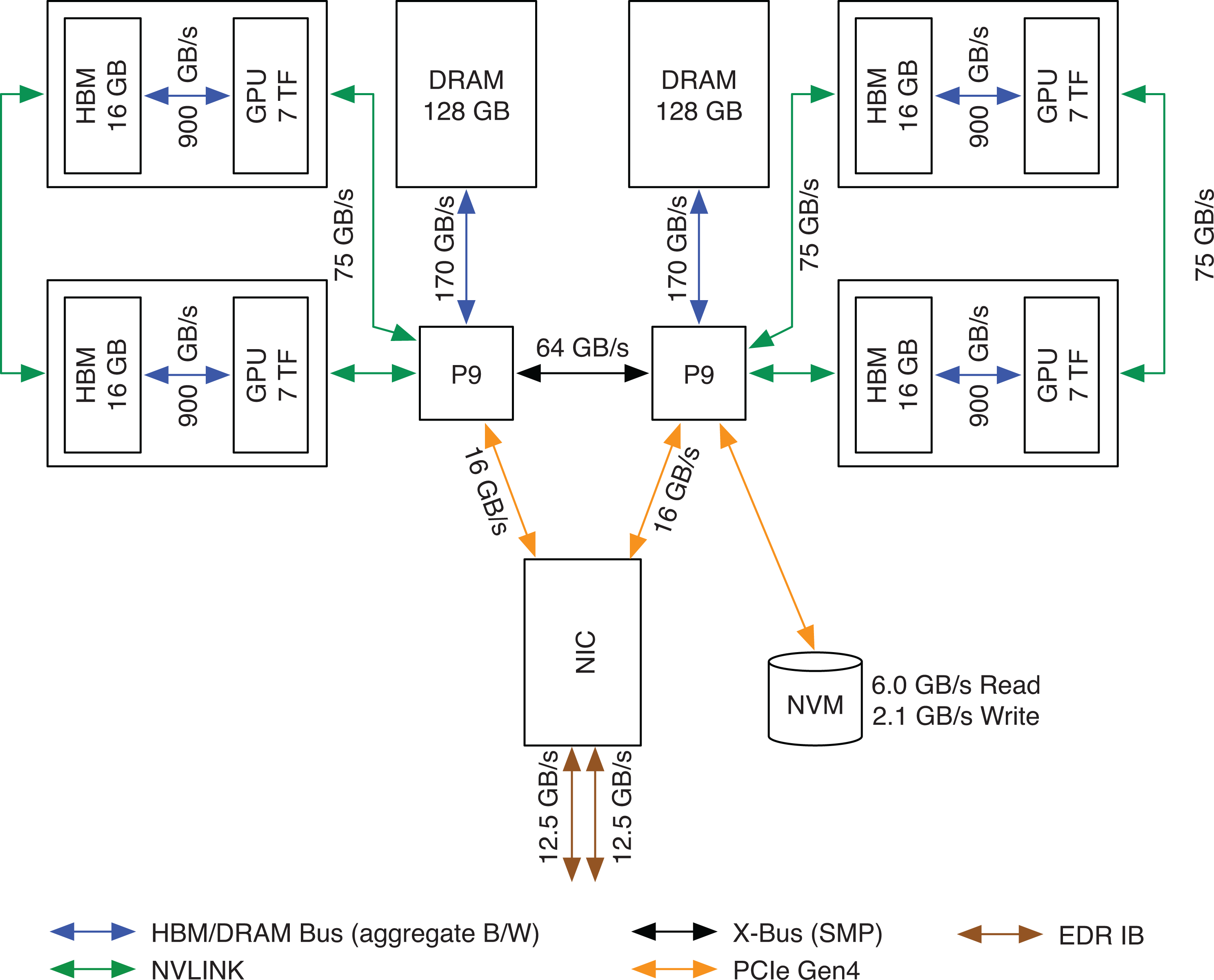
Node architecture of the Sierra supercomputer.

Racks are made up of 18 nodes, two EDR switches, and a switch with nine uplinks. Each node in the rack has a connection to each EDR switch. On Sierra each uplink connects to one of nine aggregation switches. This configuration creates a two-to-one oversubscribed network with twice the local bandwidth for nodes within a rack vs. the aggregate bi-section bandwidth between racks.

The Sierra network contains many new features (Zimmer et al., 2019), including adaptive routing, Scalable Hierarchical Aggregation and Reduction Protocol (SHARP), and hardware tag matching. We used adaptive routing during our runs, but SHARP was disabled by default. SHARP is intended for applications with many small collectives and it has mixed performance benefits on real applications.

7.2. Software environment

Our system software environment used the IBM BlueOS software stack, including LSF 10.1.0.9 as the resource manager. LBANN was built with GCC 8.3.1, CUDA 11.0.2, cuDNN 8.0.4, NCCL 2.7.8-1, and the rolling release of Spectrum MPI that was last updated on September 19th 2020.

8. Performance results

Training deep neural networks at scale involves complex trade-offs between time to solution and model quality. For example, data-parallel training can weak-scale arbitrarily by increasing the mini-batch size. However, this increase in parallelism is not free since the quality of the learned model typically degrades unless special consideration is made, e.g. by carefully adjusting the learning rate (Goyal et al., 2017). In our workflow, we divide computational resources into multiple trainers, each of which trains a model independently on a partition of the data with standard data-parallel techniques. The trainers are loosely coupled with LTFB. This strategy gave us three knobs to tune for scalable learning:

Per-trainer mini-batch size: Larger mini-batch sizes produce greater compute efficiency, but harm learning. We found 512 mini-batch size achieved the best learning and that 4096 was the upper limit of reasonable learning.

GPUs per trainer: Running with more GPUs per trainer improves run time, but reduces compute efficiency. After optimizing our GRU layers, we found that we could maintain decent computational efficiency with 256 or 512 samples per GPU. With a mini-batch of 4,096, this translated to 8 or 16 GPUs per trainer (i.e. 2 or 4 nodes per trainer).

Number of trainers: Since trainers operate independently with infrequent pair-wise communication in LTFB, they provide near-perfect “strong scaling” with respect to the data set size. For these experiments, we found that increasing the number of trainers had a beneficial effect on learning up to around 256 trainers, after which it had a slightly negative effect on learning.

A major challenge for this work was that the cWAE is poorly suited for traditional scaling techniques. As noted in Table 1, the model is not large compared to standard image and text models, ruling out model-parallel strategies. In addition, the GRU layers are tough to train and they diverge if the hyperparameters are not just right, limiting the amount of data-parallelism we could bring to bear. Achieving good results at scale required exploring a multi-dimensional optimization space to find reasonable trade-offs between performance and learning behavior.

8.1. Scaling

Achieving good scalability with LBANN required multiple levels of performance optimization. The first level involved maximizing the single-GPU performance, primarily with the GRU layer optimizations described above. See Table 4 for the effects of these optimizations.

Table 4.

Ablation study for GRU performance optimizations. Timings are for training the cWAE model on a single V100 with a 256 mini-batch, which matches the per-GPU problem size of our marquee 16 process/trainer runs with a 4,096 mini-batch.

GRU version	Mini-batch time
Optimized	37 ms
Remove multi-layer RNN API	52 ms
Remove CUDA Graph	57 ms
Downgrade to cuDNN 7 RNN API	56 ms
Disable tensor core operations	114 ms

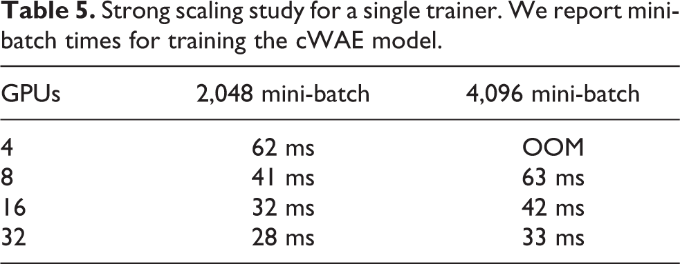
The next level was intra-trainer parallelism. In other words, we sought to maximize a trainer’s performance when running with GPUs spanning multiple nodes. Communication overheads were minimized by overlapping computation in back propagation with asynchronous gradient all-reduces (Dryden et al., 2018). With small mini-batch sizes ( $\leq 2048$ samples), either the trainer’s GPUs were starved for work with too few samples as shown in Table 5, or there were too many trainers, which reduced learning efficiency. We achieved better compute efficiency with larger mini-batches. However, our experiments with mini-batch sizes larger than 4,096 had learning that diverged, even with scaled learning rates and learning rate warmup. The best compromise between compute efficiency and learning for these experiments was a mini-batch of 4,096 and a learning rate of $0.0024$ (scaled from the learning rate used by Polykovskiy et al. (2018)).

Table 5.

Strong scaling study for a single trainer. We report mini-batch times for training the cWAE model.

GPUs	2,048 mini-batch	4,096 mini-batch
4	62 ms	OOM
8	41 ms	63 ms
16	32 ms	42 ms
32	28 ms	33 ms

The third level of parallelism was the inter-trainer parallelism enabled by LTFB. We performed an LTFB round once per epoch and the cost per round was a pair-wise synchronization between trainers, a two-way exchange of model weights, and two inference passes over a held-out data set. In prior work we have shown that LTFB maintains or improves model quality as the number of trainers increases. Thus, the LTFB algorithm enables an approximation of strong scaling with respect to a fixed sized data set. Figure 4 shows the scaling behavior of LTFB as we add more trainers, and hence add more compute nodes. The reduction in wall clock time shows near-perfect scalability to nearly all of Sierra, with 89.8% scaling efficiency with 8 GPUs per trainer and 97.7% with 16 GPUs per trainer.

Figure 4.

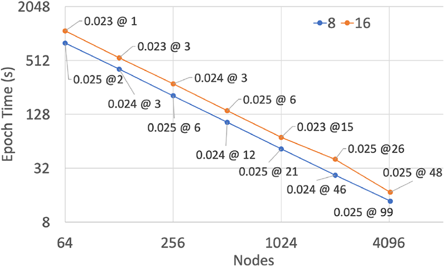
Strong scaling performance with 8 and 16 GPUs per trainer and a mini-batch size of 4,096. Data points are labeled with the number of epochs required to achieve an accuracy of 0.025 or lower.

The impact of accelerating training with LTFB in this “strong scaling” manner is dependent upon the learning behavior of the model and training algorithm. If the rate of model convergence does not scale with the reduction in time per epoch, then the time to solution will be impacted.

8.2. Total time to trained model

Using the experimental parameters described previously, Figure 5 shows the total time to solution for the subset of experiments with 16 GPUs per trainer. For these experiments we included the full data ingestion time, all time allocated to training the model, as well as all communication time related to both intra- and inter-model (LTFB) communication. The only time not reported on these graphs is the per-epoch testing forward propagation phases that were strictly used to measure the progress of the model’s learning. In addition, we adjusted the performance lines of three tests, at 4160, 2048, and 512 nodes, to account for bad compute nodes that were identified during the final full scale runs and were removed from service after that set of jobs. To normalize out the impact of failing nodes, the performance results shown here use a combination of multiple runs of the exact configuration to extrapolate the expected performance, as if we were able to rerun those final three experiments.

Figure 5.

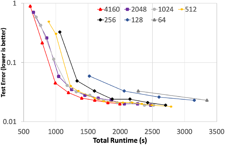
Rate of model convergence versus wall-clock time.

Figure 5 shows the rate at which the model is converging with respect to wall-clock time. Training with 256 nodes provides a significant improvement in time to solution when compared to using 64 nodes, achieving a 1.79 $\times$ speedup and a parallel efficiency of 44.65% . This speedup allows us to successfully replace the state of the art JT-VAE model that took 24 hours to train on only 1 M compounds with a much more accurate model (Table 2) that was trained in 32 minutes. However, it is significant to note that while the framework scales (see Figure 4), the model learning does not scale commensurately with the increased compute capacity. Specifically, with a maximum learnable mini-batch size of 4096 samples, there are significant limitations on scaling the number of GPUs per trainer beyond 16. In Figure 5 we see that using 4160 nodes of Sierra provides a 18% speedup over 2048 nodes, in terms of time to solution, and 2.39 $\times$ over using 64 nodes, a parallel efficiency of 3.68%. While the parallel efficiency as measured for increasing time to convergence is low, it is reflective of the model and its’ behavior during training. There are additional training techniques that may allow larger mini-batches in the future, such as the application of optimizers tuned for larger batch sizes, e.g. LAMB (You et al., 2020), or second order optimizers (Osawa et al., 2019). We also observed that I/O time almost remains constant beyond 512 nodes impacting overall scalability of end to end training.

The key innovation here is that the LBANN framework enables research into deep learning architectures at scales that were previously unobtainable. The cWAE model used in the experiment is not the only model of interest, nor is the Enamine data set the only one of interest. Model architecture exploration, hyperparameter tuning, and the vast scale of chemical space all demand frequent model training. The techniques developed in this work will allow our domain scientists to explore these possibilities at a rate that will make deep learning training “explorable-able” in near-real time and test models plus data sets that were previously intractable.

8.3. Peak performance

Using 4,160 nodes of Sierra and a mini-batch size of 4,096 samples per trainer, we were able to train the cWAE model with 1,040 and 2,080 trainers. This traded off the amount of intra-trainer parallelism and the quality of the learned model. Table 6 shows that we were able to achieve 253.3 PFLOPS and 318 PFLOPS respectively, all using tensor cores with mixed-precision training (half-precision multiplication with single-precision accumulate). Using more processes per trainer, and thus fewer trainers, improved the quality of the model, resulting in 1,040 trainers achieving a final test reconstruction error of 0.02 at 83 epochs versus 2,080 trainers achieving 0.025 at 99 epochs.

Table 6.

Peak performance training with 4,160 nodes on Sierra.

GPUs/trainer	Trainers	Epoch time	PFLOPS
16	1040	17.2 s	253.3
8	2080	13.7 s	318.0

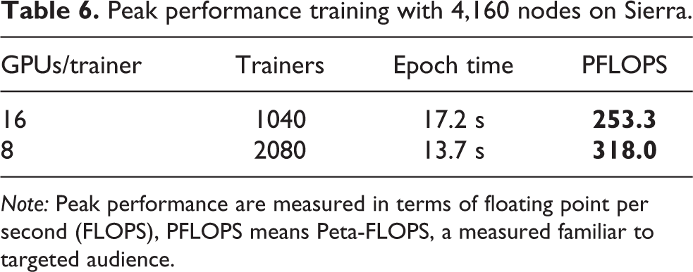
Note: Peak performance are measured in terms of floating point per second (FLOPS), PFLOPS means Peta-FLOPS, a measured familiar to targeted audience.

8.4. Power

Figure 6 shows two to three megawatt power swings during our initial full-system runs on Sierra. Sierra power is distributed from 12 wall plates that when combined are capable of fully powering the system at 11 MW. HPL power for the system was 7.44 MW. Peak power draw during our initial runs was about 5.6 MW.

Figure 6.

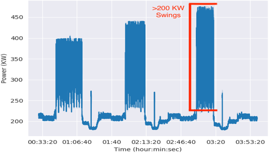
Power measured by a wall plate monitor during full system Sierra runs. At the system level, the tall, filled-in regions represent quick 2–3 MW power swings.

The chart highlights fast power swings of 200 KW at each wall plate monitor (2.4 MW total). Our utility company noticed the coarse power swings that occurred between jobs and notified us of the irregular behavior. LLNL facility staff also expressed concerns about the fast swings that occurred during training, especially about the impact on power infrastructure within the data center.

Figure 7 shows the same power profile on Sierra after we made LBANN globally asynchronous. Our changes reduced most of the high frequency swings to about 100 KW per wall plate monitor. Power variability was not fully eliminated because our LTFB exchanges still occur at regular intervals and requires pair-wise synchronization between trainers. However, stochastic variations in node performance spread these synchronizations over time, so the resulting power swings were smaller and smoother. Offsetting the exchange intervals would further smooth these curves.

Figure 7.

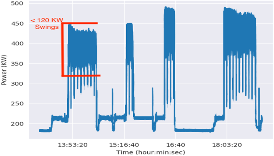
Power measure at wall plate in full system runs after LBANN was made globally asynchronous.

9. Implications

9.1. Drug design

Using an efficient cWAE model, we produce an accurate generative model with low compound reconstruction error and improve model training time from a day to 23 minutes. The cWAE model trained on Enamine chemistry yields a searchable chemical space for new compounds that are more likely to be synthesizable based on the learned representation than would be possible with arbitrary chemical permutations and with greater efficiency than would be possible through manual intervention from a human chemist. In addition, the training allows the resulting virtual libraries to have broader chemical diversity and potentially more robust compounds in different areas of chemical space; all necessary criteria to discovering novel drug entities. Directed searches are feasible for new compounds to be considered that better meet the design criteria within the molecular design loop. For example, since the cWAE model was trained in part on 1 million compounds predicted to be potent SARS-CoV-2 main protease inhibitors, the model supports a more targeted search for novel protease inhibitors.

The design of generative models remains an active area of ML research, with the need to explore new model architectures and training strategies. As more experimental feedback is obtained, there will be a need to re-tune the model to refine the chemical search. Additionally, as new pathogens emerge, beyond the SARS-CoV-2, there will be a need to re-train the generative model to optimize the search on new protein targets. Thus, the demonstration of rapid training on large data sets indicates that model building can be efficiently used to guide future drug design efforts. Fundamental challenges still remain with the need to better predict drug effects in the human body and chemical synthesis routes to efficiently make and test new molecules (Minnich et al., 2020). With the chemical space of drug-like molecules estimated to be $10^{60}$ (Reymond, 2015), there is still room to improve new compound prediction.

Furthermore, we plan to leverage an existing open source generative modeling software framework called MOSES (Polykovskiy et al., 2018) and LBANN’s compatibility with PyTorch to share generative chemistry models trained at scale with the broader research community that may not otherwise have access to large scale high performance computing resources.

9.2. Computer systems and learning at scale

Our results demonstrate that our proposed solution is capable of scaling the ML training of drug models to both an unprecedented 1.613 billion compounds and all of a pre-exascale machine. With our pressing need to discover COVID-19 drugs, an ability to quickly create high-quality ML models is critically important as this can enable fast iteration of machine learning design and thus move the model design bottleneck from computation time to human time. However, our work shows one must overcome several key challenges in systems and training technologies to realize this potential fully. In the following, we describe the key lessons learned from our work.

First, we used a 4,096 mini-batch size for training because low GPU occupancy and kernel launch overhead significantly impede the performance for smaller batch sizes. Even with this mini-batch size we needed many trainers at full system scale, which slowed convergence. GPUs are expected to gain more parallelism in future generations and kernel launch, an Amdal bottleneck, is unlikely to improve much in the future. Therefore, further decreases in training time will require either inventing additional ways to strong-scale small batch training or improve the convergence of large-batch training.

Second, we demonstrated that globally synchronous codes can cause significant power swings at scale. Most codes do not run on a full system or drive processors to high power usage like we did. However, as machines get larger and chip makers continue to find ways to save power when they are idle, larger swings will occur. Next generation supercomputers will use about three times the power of Sierra. Fugaku uses about 29 megawatts and the three exascale United State Department of Energy supercomputers are expected to have similar or slightly larger power draws. Other applications will need to become asynchronous to lower their power swings and see performance gains. GPUs may require modes that prevent them from down clocking aggressively to save power. In addition, computer centers will need to work with utility providers to increase their tolerance for large power swings and design their own equipment to handle these swings.

Third, tuning large-scale ML applications presents a complex optimization space: i.e. trade-offs between mini-batch sizes, learning rate, and other parameters used to optimize models. To explore this space, we have built a highly-scalable and performant capability that enables large-scale learning on the largest computers. This capability was leveraged in our work to allow us to quickly explore and tune multiple models, including novel models such as the cWAE. Further exploration should provide techniques to improve model quality at large scale given that initial attempts have already shown the capability to produce high quality models.

Footnotes

Acknowledgments

We thank Brian Bennion for providing the 1.613 billion compounds for training, Brandon Hong for sharing facility power data with us, and Stephen Herbein for being a friendly reviewer. We appreciate the useful discussions with Frank Di Natale, Stephen Herbein, Jeffery Mast, Luc Peterson, Benjamin Bay and Xioahua Zhang. We thank Greg Lee for debugging help and Nvidia for performance optimization conversations and support. We would like to thank Tom Benson and Nikoli Dryden from the LBANN team. We also thank all the Livermore Computing staff including Dave Dannenberg, Ryan Day, Scott Futral, and Greg Tomaschke for system access, responding to crazy requests, and making this all possible.

Declaration of conflicting interests

The author(s) declared no potential conflicts of interest with respect to the research, authorship, and/or publication of this article.

Funding

The author(s) disclosed receipt of the following financial support for the research, authorship, and/or publication of this article: This work was performed under the auspices of the U.S. Department of Energy by Lawrence Livermore National Laboratory under Contract DE-AC52-07NA27344. Funding was provided by ECP through ExaLearn, the ATOM project and LLNL ASC. LLNL-CONF-815559.

ORCID iD

Sam Ade Jacobs

Author biographies

Sam Ade Jacobs is a computer scientist and a project lead at the Center for Applied Scientific Computing (CASC) at Lawrence Livermore National Laboratory (LLNL). He received his Ph.D. in Computer Science from Texas A&M University. Sam’s broad research experiences and interests include parallel computing, large-scale data (graph) analytics, scalable machine learning, and robotics. Sam’s current work focuses on developing new algorithms for large scale neural architecture search and training with applications in image and text processing, drug design, high energy physics and other scientific applications. Sam’s work represents significant advances to the broader field of computational sciences as well as to data science by providing and maintaining unique data analytics capabilities. His approaches and tools are designed to operate on massive supercomputers at LLNL and are tested on those machines.

Tim Moon is a computer engineer at Lawrence Livermore National Laboratory. He works on scaling advanced machine algorithms to run on leadership-class HPC systems. He holds a B.S. in Physics from Rice University and an M.S. in Computational and Mathematical Engineering from Stanford University.

Kevin McLoughlin is a computational biologist at Lawrence Livermore National Laboratory. He leads the development of the Generative Molecular Design software for the Accelerating Therapeutic Opportunities in Medicine (ATOM) Consortium and created the ATOM Modeling Pipeline (AMPL), a framework for building machine learning models for drug discovery. His research spans a broad range of applications of data science to biology and medicine. Kevin received his Ph.D. in Biostatistics from U.C. Berkeley, a B.S. in Physics from Caltech and an M.S. in Physics from U.C. Santa Cruz.

Derek Jones is a computer scientist in the Global Security Computing Applications Division at Lawrence Livermore National Laboratory where he also works on behalf of LLNL in the ATOM consortium. He specializes in the development of supervised and unsupervised deep learning methodologies to 3D structure-based drug design and chemical optimization. Derek holds a B.S. in Computer Science with a dual major in Mathematical Economics and an M.S. in Computer Science from the University of Kentucky. He is currently pursuing his Ph.D. in Computer Science and Engineering at the University of California San Diego under the advisement of Dr. Tajana Rosing.

David Hysom is a computer scientist at the center for Applied Scientific Computing (CASC), Lawrence Livermore National Laboratory. He has worked in diverse problem areas, including Natural Language Processing (NLP), Bio-informatics, and Structured Adaptive Mesh Refinement Application Infrastructure (SAMRAI). He has been been working in the AI field for the past several years.

Dong H Ahn is a computer scientist. He has worked for Livermore Computing (LC) at Lawrence Livermore National Laboratory since 2001 and currently leads the next-generation computing enabling (NGCE) project within the ASC ATDM sub-program. During this period, Dong has worked on several code-development-tools and next-generation resource management and scheduling software framework projects with a common goal to provide highly capable and scalable tools ecosystems for large computing systems. Toward this goal, he has architected an extreme-scale debugging strategy that conceived the Stack Trace Analysis Tool (STAT), a 2011 R&D 100 Award winner, and the PRUNERS Toolset, a 2017 R&D 100 Award Finalist. His current interest includes scalable approaches to managing the adverse impacts of non-determinism in concurrent execution, and to HPC resource and job management. Before he joined LLNL, Dong earned a Master’s degree in Computer Science in 2001 from the University of Illinois at Urbana-Champaign and had worked for National Center for Supercomputing Applications (NCSA), as a research assistant.

John Gyllenhaal is a computer scientist at Lawrence Livermore National Laboratory (LLNL). He has been cheerfully supporting supercomputer users and helping debug the world’s most powerful supercomputers as part of Livermore Computing (LC) since 1999. John’s 1997 Ph.D. in EE focused on high-performance processor design that leveraged advanced compiler technology and was earned at the University of Illinois at Urbana-Champaign. John spent much of the 1990s writing compilers, processor simulators, and debugging tools. Much of John’s time since then has been spent leading various LLNL efforts to make compilers and development environments more powerful and useful for supercomputer users.

Pythagoras Watson is a computer scientist who works for Livermore Computing (LC) at Lawrence Livermore National Laboratory. Py has over 20 years as a high-performance computer systems administrator. He is the Advanced Technology Team Lead in charge of installing, operating, and maintaining some of the largest and fastest computer systems in the world. Py earned his B.S. in Computer Science from California State University, Chico.

Felice C Lightstone is a computational chemist and is the Group Leader of Biochemical and Biophysical Systems Group and the Program Leader of Medical Countermeasures at Lawrence Livermore National Laboratory. She is the Director of the American Heart Association’s Center for Accelerated Drug Discovery. Her research uses cutting-edge, multi-scale, in silico simulations to tackle problems in biology. A wide range of computational biology methods that employ LLNL’s high-performance computing resources are used to simulate systems from sub-atomic scale to population level. She holds undergraduate degrees in Electrical Engineering and Honors Biology and a Master’s Degree in Electrical Engineering from the University of Illinois and a Ph.D. in Chemistry from the University of California, Santa Barbara

Jonathan E Allen is an informatics scientist and project lead in the Biosecurity center at Lawrence Livermore National Laboratory (LLNL). He works on developing new software tools for pathogen characterization, modeling host response and machine learning for small molecule drug discovery. Jonathan received his Ph.D. in Computer Science from Johns Hopkins University in 2006, after conducting his thesis work at The Institute for Genomic Research (now The J. Craig Venter Institute).

Ian Karlin is a Principal HPC Strategist in the Advanced Technologies Office (ATO) in Livermore Computing (LC). He leads LC benchmarking efforts for next generation supercomputers and commodity clusters. He is also responsible for ATO strategy with the LC CTO for machine learning hardware. He serves as a Deputy in the El Capitan Center of Excellence and was the Deputy on the institutional Center of Excellence preparing codes for Sierra. He has won best papers at IPDPS 2013, Cluster 2015 and two LLNL excellence in publication awards in 2016 and 2018. He received his PhD from University of Colorado at Boulder in 2011.

Brian Van Essen is the informatics group leader and a computer scientist at the Center for Applied Scientific Computing at Lawrence Livermore National Laboratory (LLNL). He is pursuing research in large-scale deep learning for scientific domains and training deep neural networks using high-performance computing systems. He is the project leader for the Livermore Big Artificial Neural Network open-source deep learning toolkit, and the LLNL lead for the ECP ExaLearn and CANDLE projects. Additionally, he co-leads an effort to map scientific machine learning applications to neural network accelerator co-processors as well as neuromorphic architectures. He joined LLNL in 2010 after earning his Ph.D. and M.S. in computer science and engineering at the University of Washington. He also has an M.S and B.S. in electrical and computer engineering from Carnegie Mellon University.

References

Akiba

Suzuki

Fukuda

(2017) Extremely large minibatch SGD: training ResNet-50 on ImageNet in 15 minutes. arXiv preprint arXiv:1711.04325.

Blaschke

Olivecrona

Engkvist

, et al. (2018) Application of generative autoencoder in de novo molecular design. Molecular Informatics 37(1–2): 1700123.

Brookes

Park

Listgarten

(2019) Conditioning by adaptive sampling for robust design. In: K

Chaudhuri

Salakhutdinov

(eds) Proceedings of the 36th international conference on machine learning, proceedings of machine learning research, vol. 97. Long Beach, CA: PMLR, pp. 773–782.

Centers for Disease Control and Prevention (2020) 1918 pandemic (H1N1 virus). Available at: https://www.cdc.gov/flu/pandemic-resources/1918-pandemic-h1n1.html (accessed 21 April 2021).

Cho

Van Merriënboer

Gulcehre

, et al. (2014) Learning phrase representations using RNN encoder-decoder for statistical machine translation. arXiv preprint arXiv:1406.1078.

Coates

Huval

Wang

, et al. (2013) Deep learning with COTS HPC systems. In: International conference on machine learning (ICML), Atlanta, Georgia, USA, 16 June 2013.

Dean

Corrado

Monga

, et al. (2012) Large scale distributed deep networks. In: MI

Jordan

LeCun

Solla

(eds) Advances in Neural Information Processing Systems. Cambridge, MA: The MIT Press.

Dryden

Maruyama

Moon

, et al. (2018) Aluminum: an asynchronous, GPU-aware communication library optimized for large-scale training of deep neural networks on HPC systems. In: 2018 IEEE/ACM machine learning in HPC environments (MLHPC), Dallas TX, USA, 12 November 2018, New York, NY: IEEE, pp. 1–13.

Elton

Boukouvalas

Fuge

, et al. (2019) Deep learning for molecular design—a review of the state of the art. Molecular Systems Design & Engineering 4(4): 828–849.

10.

Enamine (2020) Real compounds: new chemical space for discovery. Available at: https://enamine.net/library-synthesis/real-compounds (accessed 21 April 2021).

11.

Gómez-Bombarelli

Wei

Duvenaud

, et al. (2018) Automatic chemical design using a data-driven continuous representation of molecules. ACS Central Science 4(2): 268–276.

12.

Goyal

Dollár

Girshick

, et al. (2017) Accurate, large minibatch SGD: training ImageNet in 1 hour. arXiv preprint arXiv:1706.02677.

13.

Gupta

Müller

Huisman

BJH

, et al. (2017) Generative recurrent networks for de novo drug design. Molecular Informatics 37(1–2): 1700111.

14.

Hinkson

Madej

Stahlberg

(2020) Accelerating therapeutics for opportunities in medicine: a paradigm shift in drug discovery. Frontiers in Pharmacology 11: 770.

15.

Iandola

Ashraf

Moskewicz

, et al. (2015) FireCaffe: near-linear acceleration of deep neural network training on compute clusters. arXiv preprint arXiv:1511.00175.

16.

Jacobs

Dryden

Pearce

, et al. (2017) Towards scalable parallel training of deep neural networks. In: Proceedings of machine learning on HPC environments, Denver, CO, November 2017, pp. 1–9.

17.

Jacobs

Van Essen

Hysom

, et al. (2019) Parallelizing training of deep generative models on massive scientific datasets. In: IEEE international conference on cluster computing, Albuquerque, NM, 23–26 September 2019.

18.

Jaderberg

Dalibard

Osindero

, et al. (2017) Population based training of neural networks. arXiv preprint arXiv:1711.09846.

19.

Jin

Barzilay

Jaakkola

(2018) Junction tree variational autoencoder for molecular graph generation. In: J

Krause

(eds) Proceedings of the 35th international conference on machine learning, proceedings of machine learning research, vol. 80. Stockholmsmässan, Stockholm, Sweden: PMLR, pp. 2323–2332.

20.

Keskar

Mudigere

Nocedal

, et al. (2017) On large-batch training for deep learning: generalization gap and sharp minima. In: Proceedings of the fifth international conference on learning representations, Toulon, France, 24 April 2017.

21.

Kingma

Welling

(2013) Auto-encoding variational Bayes. arXiv preprint arXiv:1312.6114.

22.

Kurth

Treichler

Romero

, et al. (2018) Exascale deep learning for climate analytics. In: SC18: international conference for high performance computing, networking, storage and analysis, Dallas, TX, 11–16 November 2018.

23.

Larsen

Woods

Marsaglia

, et al. (2018) A flexible system for in situ triggers. In: Proceedings of the workshop on in situ infrastructures for enabling extreme-scale analysis and visualization, Dallas TX, USA, 11 November 2018, New York, NY: Association for Computing Machinery, pp. 1–6.

24.

Maruyama

Van Essen

Dryden

, et al. (2020) Dihydrogen. Technical report . Livermore, CA: Lawrence Livermore National Lab (LLNL).

25.

Mathuriya

Bard

Mendygral

, et al. (2018) CosmoFlow: using deep learning to learn the universe at scale. In: Proceedings of the international conference for high performance computingnetworking, storage, and analysis, Dallas TX, USA, 12 November 2018.

26.

Maziarka

Pocha

Kaczmarczyk

, et al. (2020) Mol-CycleGAN: a generative model for molecular optimization. Journal of Cheminformatics 12(1): 2.

27.

Minnich

McLoughlin

Tse

, et al. (2020) AMPL: a data-driven modeling pipeline for drug discovery. Journal of Chemical Information and Modeling 60(4): 1955–1968.

28.

Osawa

Tsuji

Ueno

, et al. (2019) Large-scale distributed second-order optimization using Kronecker-factored approximate curvature for deep convolutional neural networks. In: 2019 IEEE/CVF Conference on Computer Vision and Pattern Recognition (CVPR), Long Beach, CA USA: IEEE, 15 June 2019, pp. 12351–12359. DOI: 10.1109/CVPR.2019.01264.

29.

Peterson

Anirudh

Athey

, et al. (2019) Merlin: enabling machine learning-ready HPC ensembles. arXiv preprint arXiv:1912.02892.

30.

Petrini

Kerbyson

Pakin

(2003) The case of the missing supercomputer performance: achieving optimal performance on the 8,192 processors of ASCI Q. In: Conference on supercomputing, SC ‘03, Phoenix, AZ, USA, 12 November 2003. Phoenix, AZ: ACM/IEEE.

31.

Polykovskiy

Zhebrak

Sanchez-Lengeling

, et al. (2018) Molecular sets (MOSES): a benchmarking platform for molecular generation models. arXiv preprint arXiv:1811.12823.

32.

Poulson

Marker

van de Geijn

, et al. (2013) Elemental: a new framework for distributed memory dense matrix computations. ACM Transactions on Mathematical Software (TOMS) 39(2): 1–24.

33.

Price

Howard

Cons

(2017) Fragment-based drug discovery and its application to challenging drug targets. Essays in Biochemistry 61(5): 475–484.

34.

RDKit (2020) RDKit: open-source cheminformatics software. Available at: https://www.rdkit.org (accessed 21 April 2021).

35.

Recht

Wright

, et al. (2011) Hogwild: a lock-free approach to parallelizing stochastic gradient descent. In: Advances in Neural Information Processing Systems, 12 December 2011. Granada, Spain: Currant Associates Inc, pp. 693–701.

36.

Reymond

(2015) The chemical space project. Accounts of Chemical Research 48(3): 722–730.

37.

Rezende

Mohamed

Wierstra

(2014) Stochastic backpropagation and approximate inference in deep generative models. arXiv preprint arXiv:1401.4082.

38.

Sanchez-Lengeling

Aspuru-Guzik

(2018) Inverse molecular design using machine learning: generative models for matter engineering. Science 361(6400): 360–365.

39.

Skalic

Jiménez

Sabbadin

, et al. (2019) Shape-based generative modeling for de novo drug design. Journal of Chemical Information and Modeling 59(3): 1205–1214.

40.

Tabe

Hardwick

Stout

(1995) Statistical analysis of communication time on the IBM SP2. Computing Science and Statistics 27: 347–351.

41.

Tolstikhin

Bousquet

Gelly

, et al. (2017) Wasserstein auto-encoders. arXiv preprint arXiv:1711.01558.

42.

Van Essen

Kim

Pearce

, et al. (2015) LBANN: Livermore big artificial neural network HPC toolkit. In: Proceedings of the workshop on machine learning in high-performance computing environments, MLHPC ‘15. New York, NY: Association for Computing Machinery. DOI: 10:1145/2834892:2834897.

43.

Vazhkudai

de Supinski

Bland

, et al. (2018) The design, deployment, and evaluation of the CORAL pre-exascale systems. In: SC18: international conference for high performance computing, networking, storage and analysis, Dallas TX, USA, 12 November 2018, New York, NY: IEEE Press, pp. 661–672.

44.

Winter

Montanari

Noé

, et al. (2019a) Learning continuous and data-driven molecular descriptors by translating equivalent chemical representations. Chemical Science 10(6): 1692–1701.

45.

Winter

Montanari

Steffen

, et al. (2019b) Efficient multi-objective molecular optimization in a continuous latent space. Chemical Science 10(34): 8016–8024.

46.

You

Hseu

Ying

, et al. (2019) Large-batch training for LSTM and beyond. In: Proceedings of the International Conference for High Performance Computing, Networking, Storage and Analysis, SC19, Denver, CO, CA, 14 November 2019, ACM/IEEE.

47.

You

Reddi

, et al. (2020) Large batch optimization for deep learning: training BERT in 76 minutes. In: Proceeding International Conference on Learning Representations, online. Available at: https://openreview.net/forum?id=Syx4wnEtvH

48.

You

Zhang

Hsieh

, et al. (2018) ImageNet training in minutes. In: Proceedings of the 47th international conference on parallel processing, Eugene, OR, August 2018, pp. 1–10.

49.

Zeldovich

(2020) How America brought the 1957 influenza pandemic to a halt. JSTOR Available at: https://daily.jstor.org/how-america-brought-the-1957-influenza-pandemic-to-a-halt/ (accessed 22 April 2021).

50.

Zhu

Zhang

Allen

, et al. (2020) Binding affinity prediction by pairwise function based on neural network. Journal of Chemical Information and Modeling 60(6): 2766–2772.

51.

Zimmer

Atchley

Pankajakshan

, et al. (2019) An evaluation of the coral interconnects. In: Proceedings of the international conference for high performance computing, networking, storage and analysis, SC ‘19. New York, NY: Association for Computing Machinery. DOI: 10:1145/3295500:3356166.

Enabling rapid COVID-19 small molecule drug design through scalable deep learning of generative models

Abstract

Keywords

1. Justification

2. Performance attributes

3. Overview of the problem

4. Current state of the art

4.1. Biology/chemistry

4.2. Large scale machine learning

5. Innovations realized

5.1. Model design

5.1.1. Model architecture

5.1.2. Model evaluation

5.2. Performance optimizations

5.2.1. Single-GPU tuning

5.2.2. Data ingestion improvements

5.2.3. Removing global synchronization

6. How performance was measured

6.1. Applications used to measure performance

6.2. Data collection

6.3. Measuring model quality

7. System and environment where performance was measured

7.1. Hardware environment

7.2. Software environment

8. Performance results

8.1. Scaling

8.2. Total time to trained model

8.3. Peak performance

8.4. Power

9. Implications

9.1. Drug design

9.2. Computer systems and learning at scale

Footnotes

Acknowledgments

Declaration of conflicting interests

Funding

ORCID iD

Author biographies

References