Sage Journals: Discover world-class research

Abstract

The cerebellum is a part of the brain that plays essential roles in real-time motor learning and control and even cognitive functions. Thanks to the large amount of anatomical and physiological data, we implemented a spiking network model of the cerebellum on Shoubu, an energy-efficient supercomputer with 1280 PEZY-SC processors at RIKEN. Our artificial cerebellum consists of more than one billion neurons, which is comparable to the whole cerebellum of a cat. Using 1008 of 1280 processors on Shoubu, we achieved real-time simulation, that is, a computer simulation of the model for 1 s completes within 1 s of the real world with temporal resolution of 1 ms. Effective performance was estimated as 68 teraflops in single-precision floating points, suggesting 2.6% of peak performance. We expect that the artificial cerebellum will be applicable to various engineering applications, such as robotics and brain-style artificial intelligence.

Keywords

Brain cerebellum spiking neuron simulation real time accelerator PEZY-SC application

1. Introduction

In humans, the brain is a complex network composed of about 10¹¹ nerve cells called neurons (Kandel et al., 2013). Neurons exchange information encoded by brief electrical pulses called spikes, meaning that the carrier of information among neurons is a bit. Neurons receive spikes from other neurons connected via junctions called synapses and accumulate and emit spikes to other neurons. The brain is not a single densely connected network. It is composed of several anatomically distinct parts, such as the cerebral cortex and the cerebellum (Figure 1(a)) that act as distinct functional modules. The whole brain is a mixture of such modules that work in synergy.

Figure 1.

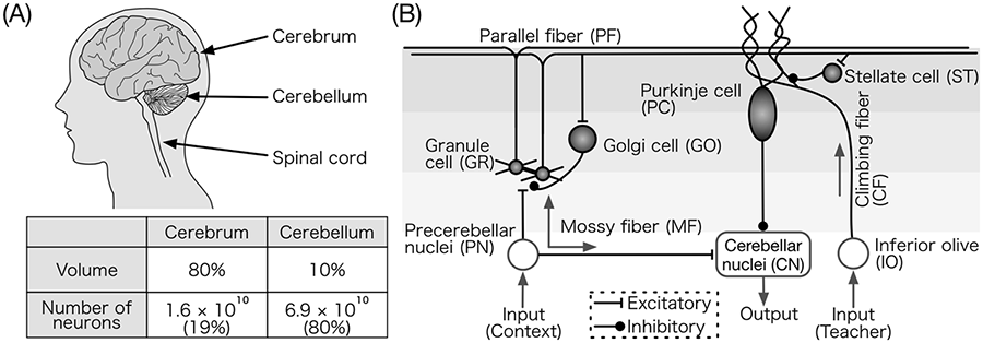
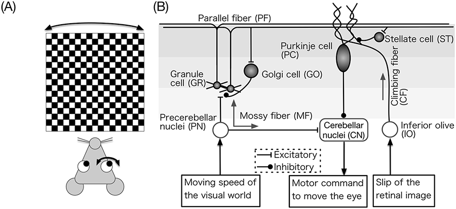
Cerebrum and cerebellum. (a) The volume and number of neurons in the cerebrum and cerebellum, respectively. The cerebellum constitutes only 10% of the whole brain volume; however, it contains approximately 80% of the brain’s neurons (Azevedo et al., 2009). (b) Schematic diagram of the cerebellar network. This network is considered a functional module called a corticonuclear microcomplex (Ito, 1984). This structure appears repeatedly and thus forms the whole cerebellar circuit. Abbreviations are also indicated.

The cerebellum is located posterior to the brain stem and is attached with the brain stem and the spinal cord (Figure 1(a)). Traditionally, the cerebellum is thought to play essential roles in motor learning and control, because when the cerebellum is damaged, severe motor deficit or ataxia is observed (Ito, 1984). Recently, however, it has been hypothesized that the cerebellum plays assistive roles in cognitive functions by organizing the cerebro-cerebellar communication loop (Ito, 2008, 2012). Moreover, the volume and number of neurons in the human cerebellum is greater by a factor of three than that of chimpanzees, the closest relatives of human beings (Herculano-Houzel and Kaas, 2011). The cerebellum likely contributes to human-specific functions, such as bipedal locomotion, intellectual communication through language, and production and utilization of tools (Lieberman, 2014). We expect that a computer simulation model of the cerebellum could be used for various engineering applications that require motor control and learning functions, such as adaptive robotics and brain-style artificial intelligence.

Fortunately, the cerebellum is one of the most studied brain regions; thus, there is a massive amount of experimental data from the molecular level to the behavioral level (Eccles et al., 1967; Ito, 1984, 2012). Such “big data” allow us to build a large-scale, realistic artificial cerebellum on a computer. Moreover, the cerebellum has two unique features. First, most cerebellar neurons are granule cells (GRs), which are the smallest neurons in the brain that are densely packed in the granular layer of the cerebellum. Second, the cerebellum has a regular and repeated anatomical structure comprised of corticonuclear microcomplexes, a unit network considered a functional module of the cerebellum (Ito, 1984). These features are advantageous to implement an artificial cerebellum efficiently on many-core accelerators.

In this study, we built a cat-scale artificial cerebellum composed of more than 10⁹ spiking neurons modeled as leaky integrate-and-fire units, which is a simple model for single neuron dynamics described by ordinary differential equations (ODEs) (Gerstner et al., 2014). We implemented it on Shoubu, an energy-efficient supercomputer with 1280 PEZY-SC Manufacturer is PEZY Computing processors installed at the RIKEN Advanced Center for Computing and Communication (ACCC) (RIKEN ACCC, 2015). Using 1008 processors, we achieved a simulation of a cat-scale artificial cerebellum in real time, which means that a simulation of the cerebellar activity for 1 s completes within 1 s of the real world, with temporal resolution of 1 ms. To realize the real-time simulation, we employed various PEZY-SC-specific techniques including the use of local memory and the reduction on cache hierarchy. We also developed a technique called noisy delayed spike transmission to reduce communication among processors via the message passing interface (MPI). Ultimately, we achieved 68 teraflops in single-precision floating points.

2. Materials and methods

2.1. Overview of the cerebellum: Structure and function

The cerebellum receives two inputs and provides one output (Figure 1(a) and (b)). One input comes from precerebellar nuclei (PN) such as pontine nuclei and nucleus reticularis tegmenti pontis (NRTP) that relay the signals from sensory organs or other brain areas. The signals are conveyed by excitatory mossy fibers (MFs) to GRs and cerebellar nuclear neurons (CNs). GRs provide excitatory inputs to Golgi cells (GOs), Purkinje cells (PCs), and molecular layer interneurons such as stellate cells (STs) via GR axon (fiber that emits the output signals) parallel fibers (PFs). GOs in turn inhibit GRs, suggesting that GRs and GOs form a recurrent network. PCs inhibit CNs, and STs inhibit nearby PCs. The output of CNs becomes the final output of the cerebellum. Another input to the cerebellum comes from the inferior olive (IO) via climbing fibers (CFs). CFs innervate to PCs and evoke very large activation on the PCs, which is thought to induce a plastic change of synaptic connections of PFs innervating the same PC, called long-term depression (LTD) (Ito et al., 2014).

The neural network shown in Figure 1(b) is considered actually as a functional module of the cerebellum called a corticonuclear microcomplex (Ito, 1984). Accumulating evidence suggests that a microcomplex is a biological counterpart of a perceptron, an artificial neural network for supervised learning (Albus, 1971; Marr, 1969; Rosenblatt, 1958). In supervised learning, a learning machine receives many pairs of a context signal and a teacher signal and learns the association between the context and the teacher. After learning, in response to a given context signal, the machine predicts the correct answer specified by the teacher signal associated with the context signal. In the cerebellum, MFs and CFs convey context and teacher signals, respectively, and learned memory is stored at PF-PC synapses by LTD.

2.2. The model

In general, our artificial cerebellum is a model of the whole cerebellum of a cat. Although the cerebellum has a 3-D structure, we flattened the z-axis and expanded the structure as a two-dimensional (2-D) sheet of 64×64 mm². We arranged the following neurons regularly on the 2-D grid: 1,073,741,824 (= 32,768×32,768) GRs, 1,048,576 (= 1024×1024) GOs, 32,768 (= 1024×32) PCs, 32,768 (= 1024×32) STs, 1024 (= 1024×1) CNs, and 1024 (= 1024×1) IOs. These neurons are the major types of cerebellar neurons considered to be part of a corticonuclear microcomplex (Ito, 1984). The size and number of neurons are consistent with the cat cerebellum. The neurons are connected according to the anatomical data of the cat’s cerebellum (Palkovits et al., 1971a, 1971b, 1971c, 1972) and modeled as spiking neurons that emit spikes for communication. Cell parameters are taken from electrophysiological data (Audinat et al., 1992; Bal and McCormick, 1997; Brickley et al., 1999; Czubayko et al., 2001; D’Angelo et al., 1995; De Schutter and Bower, 1994; Dieudonné, 1998; Kondo and Marty, 1998; Llano et al., 1991; Llinás and Yarom, 1981; Maex and De Schutter, 1998; Midtgaard, 1992; Mouginot and Gähwiler, 1995; Puia et al., 1994; Schweighofer et al., 1999; Silver et al., 1992).

2.2.1. Anatomical structure

Here, we describe the details of the network structure in a 2×2 mm² sheet, which is implemented on a single PEZY-SC processor. On a 2×2 mm² sheet, we arranged 1024×1024 GRs, 32×32 GOs, 32×1 PCs, 32×1 STs, one CN, and one IO regularly based on the following anatomical observations.

First, we describe the structure of the granular layer composed of GRs and GOs (Figure 2(b)). The GO density in the cat granular layer is approximately 1000 mm⁻³ (Lange, 1974; Palkovits et al., 1971b). Because the thickness of the cat’s granular layer is approximately 250 μm (Eccles et al., 1967), a flattened granular layer of 2×2 mm² would contain the 1000 GOs. We set the number of GOs to 1024 (= 32×32) for ease of implementation. Thus, the spacing between two nearby GOs is 64 μm. Similarly, the GR density is estimated to be approximately 10⁶ mm⁻³ (Palkovits et al., 1971b), suggesting that the flattened granular layer of 2×2 mm² would contain 10⁶ GRs. We set the number of GRs to 1,048,576 (= 1024×1024).

Figure 2.

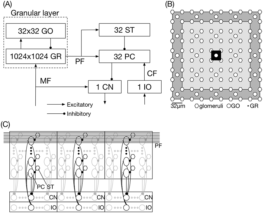
Network structure of the cerebellar model of a 2×2 mm² sheet implemented on a single processor. (a) Connectivity and the number of neurons on the sheet. (b) Spatial arrangement of glomeruli (hexagons), GOs (circles), and GRs (dots). Only the area of 320×320 μm is illustrated. The rectangle in pale gray indicates the area of the dendritic arborization (i.e. input) of the GO at the center, whereas that in dark gray, the area of the axonal arborization (i.e. output). (c) Spatial arrangement of PCs, STs, CN, and IO on a processor. PCs and STs are represented by ovals and hexagons, respectively. A thick square represents a network implemented on each processor, where 32 PCs and 32 STs are included (drawn by thick lines). We implemented only these neurons in this study, although a 2×2 mm² sheet should contain 32×32 PCs and the same number of STs (drawn by thin lines). Long horizontal lines represent PFs which provide excitatory inputs to PCs and STs. An ST inhibits the companion PC. Bottom boxes include CNs and IOs, respectively. For each processor, one CN and one IO are implemented. The 32 PCs on the same processor inhibit the CN. The IO provides excitatory inputs to the 32 PCs. GO: Golgi cell; GR: granule cell; PC: Purkinje cell; ST: stellate cell; CN: cerebellar nuclear neuron; IO: inferior olive.

Next, we describe the structure for the other neurons such as PCs, STs, CNs, and IOs (Figure 2(c)). PCs are located on the outer surface called PC layer of the cerebellum, and their density on a 1-mm² surface is approximately 330 (Palkovits et al., 1971a), suggesting that 1320 PCs would exist on a 2×2 mm² sheet. We assumed that this number is slightly smaller and set it to 1024 (= 32×32) with a cell spacing of 64 μm. In this study, for simplicity, we only implemented 32×1 PCs in the middle of the sheet; thus, a 2×2 mm² sheet provides only one output. PCs aligned parasagittally (y-axis) constitute a group called a microzone (Eccles et al., 1967). Thus, we implemented one microzone per processor. STs are small interneurons with short axons of approximately 40 μm (Eccles et al., 1967). This and the PC spacing of 64 μm suggest that an ST could inhibit only the most proximal PC; thus, we assumed the same number of STs with PCs. The cell number ratio of PCs and CNs is estimated as approximately 26:1 in cats (Palkovits et al., 1977), whereas in our model, the ratio is 32:1, which is sufficiently close with previously reported experimental results. PCs in a microzone inhibit the same CN and receive inputs from the same IO (Eccles et al., 1967). Thus, the 32 PCs on the sheet inhibit one CN while receiving inputs from one IO.

Then, we describe the inputs to the sheet and the output from the sheet. MFs convey input signals, and the number of fibers in the whole cat cerebellum is estimated to be two to four times greater than that of PCs (Palkovits et al., 1972). We assumed that the number of MFs is four times greater than PCs, and thereby considered 64×64 MFs with a regular spacing of 32 μm. These 64×64 MFs provide excitatory inputs to 1024×1024 GRs. A GR has only four dendrites (fibers that receive inputs) to receive the MF inputs, and most dendrites are shorter than 30 μm (Palkovits et al., 1971b). The short dendrites and the MF spacing suggest that a GR receives inputs from only the nearest four MFs. Because the MF spacing is 32 μm, 16×16 GRs are assumed to share the same MFs, which results in the formation of a GR cluster of 256 GRs. We consider the cluster as a functional unit of GRs. In other words, a 2×2 mm² contains 64×64 GR clusters, where each cluster has 16×16 GRs. On the other hand, a GR also receives inhibitory inputs from GOs. Here, a GR does not receive GO axons directly. A GO axon terminates at the terminal of an MF, which is also contacted by GR dendrites. This forms a structure called a glomerulus (Mugnaini et al., 1974). Thus, a GR receives inhibitory inputs indirectly via nearby glomeruli, suggesting that GRs in a cluster share the same inhibitory inputs. A glomerulus is assumed to receive inhibitory inputs from the nearest 5×5 GOs because the axonal arborization of a GO is as large as 300×300 μm² (Dieudonné, 1998) with a cell spacing of 64 μm of GOs. We set the connection probability at 0.08 such that the average number of GO axons innervating a glomerulus is 2.0 $(\approx 5 \times 5 \times 0.08)$ . For simplicity, we also assumed that a GR received only one MF, suggesting that only 1,048,576 MFs were implemented, and a GR received two inhibitory inputs.

A GO is assumed to receive excitatory inputs from 7×7 GR clusters because the dendritic arborization of a GO is estimated as large as 200×200 μm² (Dieudonné, 1998), and GO inhibition produced by PF stimulation extends no farther than 200 μm (Eccles et al., 1967). We set the connection probability to 0.2, suggesting that a GO receives inputs from approximately 2500 GRs ( $\approx 256 \times 49 \times 0.2$ ). On the other hand, a GO inhibits nearby 9×9 GR-clusters as described previously.

A PC receives excitatory inputs from nearby 32×8 GR-clusters, because the PC dendrites extend by approximately 292 μm (Palkovits et al., 1971a), and PF stimulation could evoke excitation at 1 mm distal PCs (Vranesic et al., 1994). A PC receives an inhibitory input from the nearest ST, as described above. A PC also receives an excitatory input from a single IO (Eccles et al., 1967). In turn, a PC inhibits one CN.

An ST is assumed to receive the same excitatory inputs from nearby 32×8 GR-clusters with the companion PC and inhibits the companion PC.

A CN receives excitatory MF inputs and inhibitory inputs from PCs. We assumed that a CN receives 128 MFs and inhibitory inputs from 32×1 PCs arranged parasagittally (Palkovits et al., 1977).

2.2.2. Neuron equations

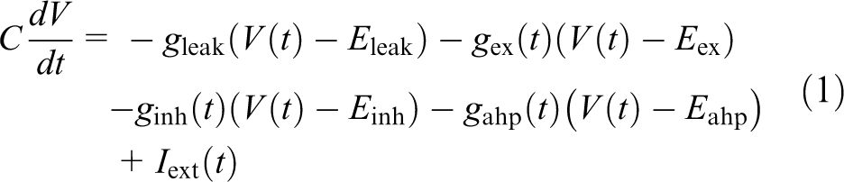
Neurons are modeled as leaky integrate-and-fire units, a simple mathematical description of spiking neurons, as follows (Gerstner and Kistler, 2002):

\begin{matrix} C \frac{dV}{dt} & = - g_{leak} (V (t) - E_{leak}) - g_{ex} (t) (V (t) - E_{ex}) \\ - g_{inh} (t) (V (t) - E_{inh}) - g_{ahp} (t) (V (t) - E_{ahp}) \\ + I_{ext} (t) \end{matrix}

(1)

where $V (t)$ is membrane potential (the internal state of the neuron), C is membrane capacitance, $g_{leak}$ is leak conductance, $g_{ex} (t)$ and $g_{inh} (t)$ are excitatory and inhibitory synaptic conductances, respectively; $g_{ahp} (t)$ is conductance for afterhyperpolarization (AHP); $E_{leak}$ , $E_{ex}$ , $E_{inh}$ , and $E_{ahp}$ are voltages called the reversal potentials; and $I_{ext}$ is the external current representing spontaneous activity. When the membrane potential exceeds a constant θ, that is, a threshold, the neuron is assumed to emit a spike, and then the membrane potential is reset to $E_{leak}$ . Parameter values for each cell type are summarized in Table 1.

Table 1.

Summary of cell parameters.

Parameter	Neuron type
	GR	GO	PC	ST	CN	IO
$θ_{spike}$ (mV)	−35.0	−52.0	−55.0	−55.0	−38.8	−50.0
C (pF)	3.1	28.0	107.0	107.0	122.3	10.0
$g_{leak}$ (nS)	0.43	2.3	2.32	2.32	1.63	0.67
$E_{leak}$ (mV)	−58.0	−55.0	−68.0	−68.0	−56.0	−60.0
${\bar{g}}_{ex}$ (nS)	0.18	45.5	0.7	0.7	50.0	1.0
${\bar{g}}_{ex}$ (nS)	0.025	30.0	—	—	25.8	—
$E_{ex}$ (mV)	0	0	0	0	0	0
${\bar{g}}_{inh}$ (nS)	0.028	—	1.0	—	30.0	0.18
$E_{inh}$ (mV)	−82.0	—	−75.0	—	−88.0	−75.0
${\bar{g}}_{ahp}$ (nS)	—	—	0.1	0.1	50.0	1.0
$E_{ahp}$ (mV)	—	—	−70.0	−70.0	−70.0	−75.0
$τ_{ahp}$ (ms)	—	—	5.0	2.5	2.5	10.0
$I_{ext}$ (nA)	—	0.006	0.18	0.07	0.2	—

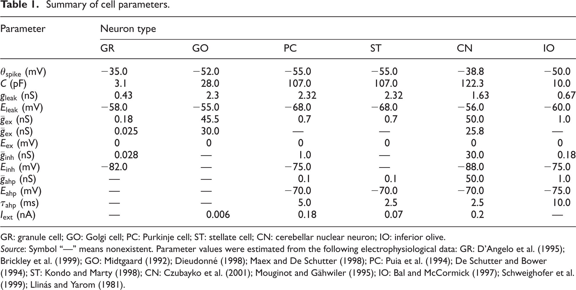
GR: granule cell; GO: Golgi cell; PC: Purkinje cell; ST: stellate cell; CN: cerebellar nuclear neuron; IO: inferior olive.

Source: Symbol “—” means nonexistent. Parameter values were estimated from the following electrophysiological data: GR: D’Angelo et al. (1995); Brickley et al. (1999); GO: Midtgaard (1992); Dieudonné (1998); Maex and De Schutter (1998); PC: Puia et al. (1994); De Schutter and Bower (1994); ST: Kondo and Marty (1998); CN: Czubayko et al. (2001); Mouginot and Gähwiler (1995); IO: Bal and McCormick (1997); Schweighofer et al. (1999); Llinás and Yarom (1981).

When a neuron emits a spike, the spike is transmitted to other neurons through their synaptic connections. We call the sender a presynaptic neuron and the receiver a postsynaptic neuron. The postsynaptic neuron changes the synaptic conductance as follows:

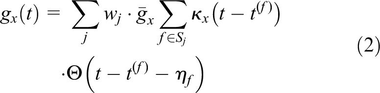
\begin{matrix} g_{x} (t) & = \sum_{j} w_{j} \cdot {\bar{g}}_{x} \sum_{f \in S_{j}} κ_{x} (t - t^{(f)}) \\ \cdot Θ (t - t^{(f)} - η_{f}) \end{matrix}

(2)

where x is either excitatory (ex) or inhibitory (inh) depending on the polarity of the presynaptic neuron, ${\bar{g}}_{x}$ is peak conductance, $w_{j}$ is a synaptic weight that represents the connection strength with the presynaptic neuron j, $S_{j}$ is a set of spikes elicited by presynaptic cell j, $t^{(f)}$ is the spike time for the fth spike, $κ_{x} (t)$ is an exponential kernel, $Θ (t)$ is the Heaviside step function, and $η_{f}$ is a randomly generated delay incorporated in the spike transmission. Synaptic transmission is noisy and therefore has certain delays. We included the delay effect explicitly in the model. The exponential kernels used in the present study are summarized in Table 2. The parameters are taken from electrophysiological data. Some neurons have several different synaptic inputs of the same polarity, for example, α-amino-3-hydroxy-5-methyl-4-isoxazolepropionic acid (AMPA) type and N-methyl-D-aspartate type excitatory inputs. In this case, we implemented only AMPA type. Some synaptic inputs are expressed by a sum of exponential functions rather than a single exponential function. In this case, we used only the component with the smallest time constant.

Table 2.

Summary of synaptic functions.

Neuron type	Equation
GR	$κ_{ex} (t) = e^{- t / 1.2}$
	$κ_{inh} (t) = e^{- t / 7.0}$
GO	$κ_{ex} (t) = e^{- t / 1.5}$
PC	$κ_{ex} (t) = e^{- t / 8.3}$
	$κ_{inh} (t) = e^{- t / 10.0}$
ST	$κ_{ex} (t) = e^{- t / 8.3}$
CN	$κ_{ex} (t) = e^{- t / 9.9}$
	$κ_{inh} (t) = e^{- t / 42.3}$
IO	$κ_{ex} (t) = e^{- t / 10.0}$

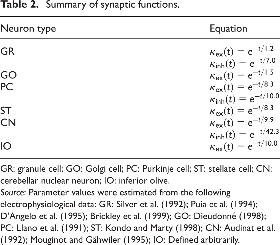
GR: granule cell; GO: Golgi cell; PC: Purkinje cell; ST: stellate cell; CN: cerebellar nuclear neuron; IO: inferior olive.

Source: Parameter values were estimated from the following electrophysiological data: GR: Silver et al. (1992); Puia et al. (1994); D’Angelo et al. (1995); Brickley et al. (1999); GO: Dieudonné (1998); PC: Llano et al. (1991); ST: Kondo and Marty (1998); CN: Audinat et al. (1992); Mouginot and Gähwiler (1995); IO: Defined arbitrarily.

The conductance for the AHP is given by

g_{ahp} (t) = \exp (\frac{- (t - \hat{t})}{τ_{ahp}})

(3)

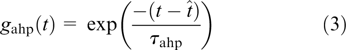
where $τ_{ahp}$ is the time constant of the AHP, and $\hat{t}$ is the last firing time of the neuron (Gerstner et al., 2014).

2.2.3. Synaptic weights

Neurons are connected at synapses with certain strength depending on the pre- and postsynaptic neurons. The synaptic weights are set manually to satisfy (1) the maximal firing rate (the number of spikes/s) becomes less than 100 spikes/s for any neurons and (2) GRs and GOs exhibit temporally modulating activity. The parameter values are summarized in Table 3.

Table 3.

Summary of synaptic weights.

Presynaptic	Postsynaptic
	MF	GR	GO	PC	ST	CN
MF	—	28.2	—	—	—	3.3
GR $(\times 10^{- 6})$	—	—	$0.43$	$1.6$	$0.75$	—
GO	—	0.96	—	—	—	—
PC	—	—	—	—	—	0.063
ST	—	—	—	8.5	—	—
IO	—	—	—	1.0	—	—

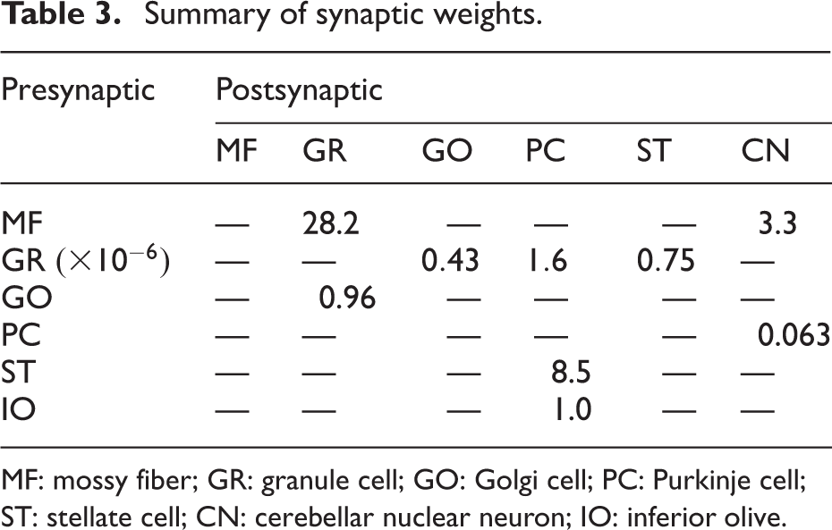
MF: mossy fiber; GR: granule cell; GO: Golgi cell; PC: Purkinje cell; ST: stellate cell; CN: cerebellar nuclear neuron; IO: inferior olive.

The main purpose of this study is to implement a large-scale cerebellar model that works in real time on Shoubu; therefore, we did not implement synaptic plasticity in the model.

2.3. Numerical method

ODEs for membrane potentials were solved by the second-order Runge–Kutta method with temporal resolution $Δ t$ of 1 ms. Conductances were discretized with the same time resolution and the following equation was derived:

\begin{matrix} g_{x} (t) & = \sum_{j} w_{j} \cdot {\bar{g}}_{x} \sum_{f \in S_{j}} κ_{x} (t - t^{(f)}) \\ \cdot Θ (t - t^{(f)} - η_{f}) \\ = κ_{x} (- Δ t) g_{x} (t - Δ t) \\ + Δ t {\bar{g}}_{x} \sum_{j} w_{j} s_{j} (t - η_{f}) \end{matrix}

(4)

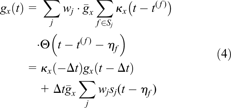
where $s_{j} (t)$ is 1 if presynaptic neuron j emits a spike at time t, otherwise 0.

2.4. PEZY-SC processor overview

A PEZY-SC processor is an accelerator composed of 1024 multiple instruction, multiple data cores called processing elements (PEs) built by PEZY Computing K.K. (Ando, 2014; Aoyama et al., 2016; Ishii, 2015; Yoshifuji et al., 2016). Figure 3 shows the schematic organization of the processor. One PE can issue eight threads. Four PEs and two L1 caches (2 KiB) are grouped as a village. Four villages with 64 KiB L2 cache constitute a city, 16 cities with 2 MiB L3 cache constitute a prefecture, and four prefectures with external DDR4 memory constitute the whole processor.

Figure 3.

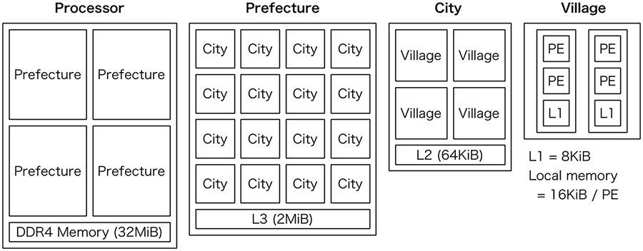
Schematic organization of a PEZY-SC processor. The processor has 1024 MIMD cores (PEs) and hierarchical L1, L2, and L3 data caches. Details are given in the text. The figure was recreated from Ando (2014) and Ishii (2015). PE: processing element; MIMD: multiple-instruction multiple-data.

Programs are written in C with a set of original application programming interfaces that resemble OpenCL (Munshi et al., 2011).

2.5. Implementation on PEZY-SC processors

We implemented our artificial cerebellum on Shoubu, a Zettascaler-1.4 supercomputer built by PEZY Computing K.K. and ExaScaler, Inc. installed at RIKEN ACCC ((Tokyo, Japan). Shoubu contains 1280 PEZY-SC processors; thus, we split the model into 1024 pieces using 1024 processors. Specifically, we split the 64×64 mm² sheet into 32×32 pieces, and we assigned each 2×2 mm² sheet to a single processor. By this assignment, each processor calculated 1,048,576 GRs, 1024 GOs, 32 PCs, 32 STs, one CN, and one IOs. One PEZY-SC processor consists of 1024 PEs. For each PE, we assigned 1024 GRs and one GO. We also assigned one PC and one ST for 32 of 1024 PEs and one IO and one CN for 1 PE. Unfortunately, 272 of 1280 processors were unavailable due to system maintenance. Therefore, we only used 1008 processors while eliminating an edge of 2×32 mm², and we simulated the 62×64 mm² sheet.

Neighboring processors communicated via MPI to exchange spike information.

2.6. Techniques for efficient simulation on PEZY-SC processors

We employed several techniques to improve performance on the PEZY-SC processors.

2.6.1. Local memory

Each PE contains 16 KiB of memory shared with a stack area called local memory, which can be used freely to store some local information. We used 12 of the 16 KiB to store neuron-local information while leaving 4 KiB for the stack area. Specifically, we stored three float variables, membrane potential, and excitatory and inhibitory synaptic conductances for 1024 GRs, thereby consuming 12 KiB memory. Using local memory allows us to avoid unnecessary memory access for information that does not require communication between neurons, such as the three float variables. To limit the stack size of each PE to no more than 4 KiB, we could use only four threads per PE, although one PE can issue eight threads.

2.6.2. Reduction of synaptic inputs on cache hierarchy

Calculation of synaptic inputs from GRs to a PC via PFs takes time. PEZY-SC has a hierarchical cache structure, that is, L1 for a pair of PEs, L2 for 16 PEs, and L3 for 256 PEs (Figure 3). We used the cache hierarchy efficiently. Since 32 PCs are assigned to a processor, we calculated eight PCs for each prefecture (Figure 3). A PC receives PF inputs from 1024×8×32 = 262,144 GRs with their connection weights, which is comparable to experimental data (Shepherd, 2004). Each PF has an 8-bit synaptic weight; thus, 128 KiB memory is necessary to store the weight values. We also require the spike data of the GRs, which consume 16 KiB because a spike is represented and packed as a bit. Each prefecture has 2 MiB data cache, so we can store the synaptic weights of eight PCs.

The actual reduction was performed as follows. We used all 256 PEs on one prefecture to perform reduction for one PC. The first reduction was performed using 1024 threads to generate 1024 single-precision floating points, which is sufficiently small to be stored in L2 cache. The second reduction was performed using one thread on one PE to sum 1024 floating points. We repeated this procedure eight times to complete eight PCs. We tested several different reduction algorithms; however, this simple method was the fastest.

2.6.3. Packing spike data and asynchronous on communication

On a PEZY-SC processor, it is mandatory to reduce/hide the time for kernel execution and data transfer between the host (CPU) and the device (PEZY-SC processor). First, to reduce the size of the spike data to be exchanged between the device and the host, we represented spikes by bits and packed the spikes of 64 GRs into an unsigned long variable. We only used a buffer of 128 KiB to store all GRs on a processor, whereas a naive implementation with an array of 1,048,576 integer variables requires a 32 times larger memory area. Second, kernel execution was performed on the device and spike exchange via MPI on the host in parallel using asynchronous MPI communication and double buffering of the spike buffer.

2.7. Reducing communication via MPI

Neurons on the edges of a sheet calculated by a processor must receive spikes from neighboring neurons calculated by the neighboring processors. For this purpose, we arranged PEZY-SC chips on a 2-D grid similar to tiling (Figure 4). Communication was performed by MPI via InfiniBand FDR using MVAPICH2-2.0 installed on Shoubu. Each chip communicates with the eight neighboring chips to exchange spike data. To reduce the data size, we partially eliminated the unnecessary portion before transmitting data.

Figure 4.

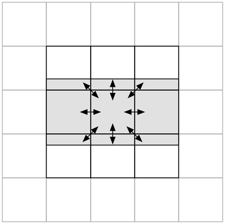
Commutation between chips via MPI. PEZY-SC chips are virtually arranged on a 2-D grid, where a square represents a PEZY-SC chip. Only the nine chips in the center are represented, whereas the surrounding chips are drawn in pale gray. The center chip communicates with the eight neighboring chips (shown by arrows) while requesting only the spike data of GRs in the shaded region. MPI: message passing interface; GR: granule cell.

In principle, communication between adjacent processors must be performed for each time step, that is, every 1 ms. Communication between processors for the spike exchange is performed via MPI, which can occupy a large portion of the total computational time. Thus, reducing the amount of communication is indispensable for real-time simulation of large-scale neural network models. We also developed a new technique to reduce communication via MPI, which we refer to as noisy delayed spike transmission (Figure 5).

Figure 5.

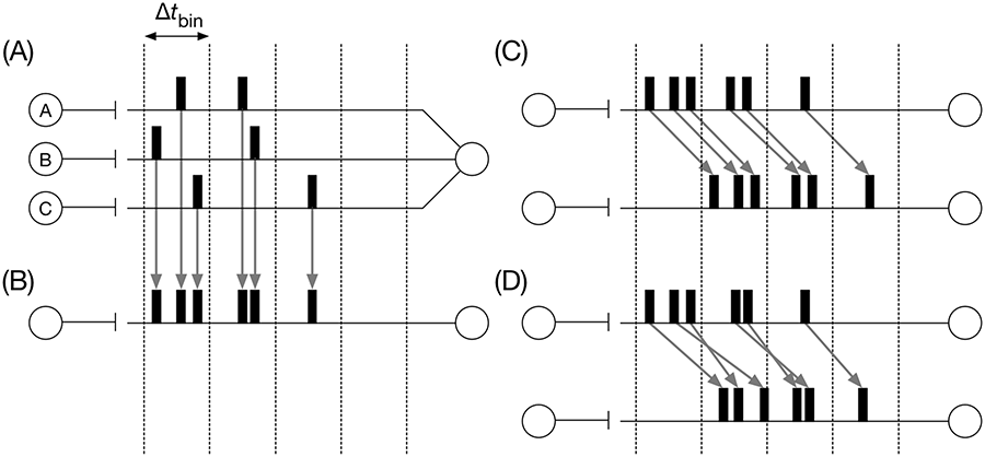
Noisy delayed spike transmission. (a) An example. Three presynaptic neurons A, B, and C send spikes to a postsynaptic neuron. The long horizontal lines represent the dendrites of the postsynaptic neuron, and black squares on the lines represent spikes emitted by the corresponding presynaptic neuron. $Δ t_{bin}$ is a time bin specified arbitrarily. For example, in the first time bin, neuron B emits a spike first, followed by neurons A and B. (b) Faithful spike transmission. Spikes are transferred to the postsynaptic neuron immediately while preserving the spike timing order. (c) Delayed spike transmission. The spikes are transferred while preserving the order, but the transmission is delayed uniformly. The top sequence is the same as in B, and the bottom sequence is the delayed sequence. (d) Noisy spike transmission. Transmission is delayed randomly for each spike; thus, the order is no longer preserved. In other words, we have made an assumption whereby the order of the spikes in each $Δ t_{bin}$ is not important due to biological noise.

The spike exchange must be performed, in principle, for each time step. However, this is only necessary when the spikes are faithfully transmitted and integrated at synapses without delays. In the biological brain, spike transmission and synaptic integration are noisy and delayed. For example, in rat cerebellar PCs, proximal PF stimulation evokes a synaptic current with a minimal latency of 1.9 ms, and then the current reaches its peak after 2.0 ms on average (Konnerth et al., 1990). Overall, the latency from the onset of stimulation to the peak current is approximately 4 ms. We assumed the same latency of 4 ms for all neurons. This means, for each postsynaptic neuron, incoming spikes from a presynaptic neuron within a time window of 4 ms are indistinguishable; thereby, the temporal order of the spikes is not important. On the other hand, neurons can emit spikes typically in a range of 0 to 100 spikes/s. Once a neuron emits a spike, the neuron cannot emit the next spike for a few millisecond, which is referred to as a refractory period. In our model, we set parameters so that all neurons emit spikes maximally at 100 spikes/s, resulting in a minimal interspike interval of 10 ms, which is greater than 4 ms. These observations allow us to perform the spike exchange between processors for each 4 ms but not for each 1 ms, because neurons emit at most one spike for each 4 ms, and spikes incoming within the 4 ms time window are indistinguishable.

The exact procedure is as follows. We split the outermost loop with respect to time with $Δ t = 1$ ms into a double loop. The inner loop counts 4 ms with $Δ t = 1$ ms and is calculated on the device (i.e. a PEZY-SC processor), whereas the outer loop counts up with $Δ t_{bin} = 4$ ms on the host. The device calculates the neural activity for 10 ms and stores the emitted spikes in a buffer, whereas the host reads the buffer of the spikes from the device, exchanges the buffer, and writes the buffer to the device for each 4 ms to calculate the next 4 ms. For consistency, when we calculated equation (2), we generated a random number from 0 to 4 for each spike as a random delay, decayed the spike with respect to the delay, and summed the spikes as a convolution.

In summary, we reduced the amount of MPI communications by one-quarter by assuming a minimal interspike interval of 4 ms for each neuron and spike transmission with random delay up to 4 ms. We could increase the value of $Δ t_{bin}$ to obtain further speedup, if we ignored the biological plausibility of the transmission delay.

3. Results

3.1. Performance

We first conducted a computer simulation of the resting state of our artificial cerebellum. To do so, we injected Poisson spikes of constant 15 spikes/s and 1.5 spikes/s to MF signals and CF signals, respectively. Poisson spikes are a sequence of spikes in time, where the average number of spikes for a certain period is fixed, for example, 15 spikes/s as in the simulation, and the actual spike timing for each spike is given uniformly at random within the period (Gerstner et al., 2014). In other words, only the number of spikes transmitted is meaningful information in Poisson spikes. We measured the computational time spent for the simulation of the resting state activity of 1 s. We obtained an average record of 0.783 s, which is faster than real time. We also counted the number of additions and multiplications at the C source code level. We found that the total number is approximately 68×10⁹ for 1 s simulation, suggesting 68 teraflops. The peak performance of Shoubu with 1008 processors is 2.6 petaflops, indicating that the effective performance of our artificial cerebellum in the resting state would be 2.6%.

3.2. Weak scaling property

Next, we changed the size of the simulated cerebellar network while varying the number of processors. In other words, we analyzed the weak scaling property. We tested the following four settings: four processors simulating 4×4 mm², 16 processors simulating 8×8 mm², 64 processors simulating 16×16 mm², and 256 processors simulating 32×32 mm². For each setting, the elapsed time increased to 0.726, 0.730, 0.737, and 0.740 s, respectively, for the simulation of 1 s, and for 1008 processors, the elapsed time was 0.783 s. Thus, the present model shows good weak scaling.

3.3. Computer simulation in a realistic scenario

Then, we carried out a computer simulation of the artificial cerebellum in a realistic scenario. We adopted simple motor control mediated by the cerebellum, that is, optokinetic response (OKR) eye movements (Figure 6). OKR is an oculomotor reflex in which the eye moves in the same direction as the visual world’s movement to stabilize the retinal image. In a standard protocol for OKR experiments, the subject is exposed to a check-patterned screen rotating slowly and sinusoidally in the horizontal direction, and the amplitude of the eye movement is analyzed (Figure 6(a)). The amplitude of the eye movement can increase adaptively by exposing the eye to a moving visual screen continuously for hours, which is called OKR adaptation. In this study, we did not consider this adaptation. We focused on only network dynamics during OKR.

Figure 6.

General overview of OKR. (a) Illustration of an OKR experiment (Shutoh et al., 2006). An animal is exposed to a check-patterned screen rotating slowly and sinusoidally. The animal’s eye moves to the same direction of the screen movement unconsciously, because this is a reflex. If the animal is exposed to the visual stimulus for a while, the eye movement becomes larger, in order to better follow the screen movement. (b) Input to the cerebellum and the output from the cerebellum in OKR adaptation. MFs convey the information of the screen movement, specifically, the velocity, whereas CFs convey the information of the slip of the visual image on the retina. The activity of CNs drives the downstream oculomotor neurons that move the eyeball. OKR: optokinetic response; MF: mossy fiber; CF: climbing fiber; CN: cerebellar nuclear neuron.

OKR is one of the simplest reflexes; thus, the cerebellar mechanism has been studied intensively. In OKR, the visual world movement, specifically the velocity of the movement, is sensed by the retinal neurons, and the information is conveyed by MFs to the cerebellum via the PN (NRTP in OKR). The retinal slip information is also sensed by retinal neurons and conveyed by CFs via the IO, which acts as an error signal to the cerebellum and triggers the induction of LTD at PF-PC synapses. The CN output drives the oculomotor neurons that move the eye (Figure 6(b)).

We conducted a computer simulation of OKR as follows. MF signals representing visual world movement were modeled as Poisson spikes with a sinusoidally modulating firing rate from 0 to 30 spikes/s in a period of 6 s (Figure 7(a)). The firing rate is consistent with cat data (Maekawa et al., 1981), and this period is typically used in standard experiments (Shutoh et al., 2006). On the other hand, CF signals representing retinal slip were modeled as Poisson spikes with a sinusoidally modulating firing rate from 0 to 3 spikes/s in the same period, according to experiments (Figure 7(b)) (Nagao, 1988). We fed those spike trains to the model for 2 min (Shutoh et al., 2006) corresponding to 20 cycles of screen rotation, obtained the spike data of all neurons, and examined the output of the network, that is, the activity of the CN. For the simulation, the whole network was not necessary. We used only one processor and one 2×2 mm² sheet.

Figure 7.

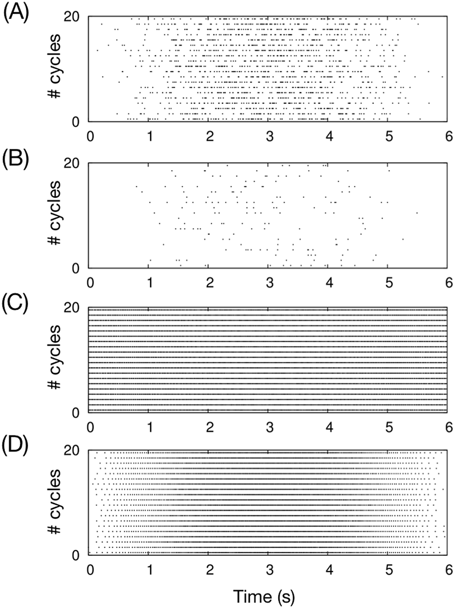
Spike patterns of an MF (a), a CF (b), a PC (c), and a CN (d) in the OKR simulation for 20 cycles. For each panel, the horizontal axis represents time in seconds, and the vertical axis represents the cycle number. A black dot represents a spike that the neuron emitted at the time of the cycle. The MF, CF, and CN emit spikes sinusoidally in phase, whereas the PC emits spikes with little modulation. MF: mossy fiber; CF: climbing fiber; PC: Purkinje cell; CN: cerebellar nuclear neuron; OKR: optokinetic response.

Figure 7 shows the result. In response to the sinusoidally modulating MF and CF signals (Figure 7(a) and (b)), GRs and GOs also emit spikes in phase with the MF signals. STs emit spikes in phase because they receive excitatory inputs from GRs, whereas PCs exhibited little modulation in their firing rate, because they receive both excitatory and inhibitory inputs from GRs and STs, respectively (Figure 7(c)). The average firing rate of PCs was 50 spikes/s, which is comparable to animal experiments. The CN emits spikes in phase with the MF signals by receiving the modulating MF signals and PC activity without modulation. The firing rate was modulated from 10 to 80 spikes/s. These activity patterns are consistent with OKR animal experiments (Kitama et al., 1999; Nagao, 1988; Shutoh et al., 2006). These results suggest that our artificial cerebellum reproduces the dynamics of the cerebellar network in a realistic scenario.

4. Discussion

High-performance neurocomputing is an emerging field in neuroscience. Various types of technology have been adopted, including supercomputers, such as the K-computer (Kunkel et al., 2014) and JuQueen (IBM; Zaytsev et al., 2015), graphics processing units (GPUs), field-programmable gate arrays (FPGAs), and dedicated hardware called neuromorphic chips (Furber et al., 2014; Merolla et al., 2014). The present article adds the PEZY-SC processor to this list. The Human Brain Project (2013) has been leading this field. This project aims to replicate and simulate the entire human brain using a supercomputer. The present study follows the same direction while focusing on the cerebellum. Several groups have been implementing small-scale cerebellar models on GPUs (Casellato et al., 2015; Garrido et al., 2013; Gosui and Yamazaki, 2016; Li et al., 2013; Naveros et al., 2014) and FPGAs (Luo et al., 2016). The many-core architecture of the PEZY-SC processor is suitable for simulating a large number of identical neurons, such as cerebellar GRs. In the present study, we elaborated a much large-scale cerebellum composed of one billion neurons, and now this size is comparable to the entire cat cerebellum.

The basic structure of the present model inherits that of our previously published cerebellar models (Gosui and Yamazaki, 2016; Luo et al., 2016; Yamazaki and Igarashi, 2013; Yamazaki and Nagao, 2012; Yamazaki et al., 2015). This allowed us to build this large-scale model reliably while comparing dynamics with previous models. As a result, our model demonstrated qualitatively similar dynamics to the previous models, which implies that the present study does not provide new insights into cerebellar mechanisms. In this sense, the simulation results reported in the present article might be considered a benchmark that justifies the overall dynamics of the present model. This would be one potential problem of the present article; however, this comes from another potential problem, that is, the lack of learning mechanisms. While we understand that learning is an essential function of the cerebellum, in this article, we have focused on an efficient implementation of the cerebellar circuit with one billion neurons on PEZY-SC processors. Implementation of learning mechanisms, particularly PF-PC LTD and LTP, is our next target. One challenge will be how to update so many synaptic weights for each time step efficiently while retaining real-time simulation, and we assume that some pipelining techniques to overlap reading, modifying, and writing memory will be required. On the other hand, once we succeed in implementing learning capability, the new model will successfully expand our knowledge of the cerebellar computation, as our previous models have done. For example, Yamazaki and Nagao (2012) proposed a unified computational principle of the cerebellum for gain and timing control, and Gosui and Yamazaki (2016) reproduced long-term memory consolidation in OKR adaptation by assuming two different synaptic plasticity sites in the cortex and nuclei. Luo et al. (2016) are exploring the possibility of applying our cerebellar model to medical applications. Furthermore, the present model has a huge advantage over our previous models, that is, its size. The present model could be applied to integrate many sensory and motor inputs from external systems including other brain models or robots and return many motor signals and predicted sensory signals to those systems simultaneously in real time. Overall, although the present model may be immature due to the lack of learning capability and somewhat unrealistic, we believe that the model can provide future insights into understanding the cerebellum.

Using PEZY-SC processors, we were able to implement the large-scale network efficiently, resulting in real-time simulation. In particular, local memory provides a means to turn the processor into a kind of neuromorphic chip. A neuromorphic chip, such as SpiNNaker (Furber et al., 2014) and TrueNorth (IBM; Merolla et al., 2014), comprises many computational cores, and each core has its own private memory. A core and the memory are located side by side; therefore, the chip can avoid bottle necks in global memory access. The use of local memory on the PEZY-SC processors provides the same functionality. On the other hand, in a neuromorphic chip, data transfer must be made via routing between cores. This could be a bottle neck when a large amount of data, for example, synaptic weights, must be read/written in bulk mode. A PEZY-SC processor also uses conventional DDR4 memory, which enables efficient global memory access. Thus, the architecture of a PEZY-SC processor seems ideal for a practical large-scale neural network simulation.

We developed noisy delayed spike transmission to reduce the amount of inter-node communications via MPI by assuming that spike transmission and invoking postsynaptic potentials are randomly delayed by a few millisecond due to biological background noise and several intracellular mechanisms. However, this means that, if a neural network model employs synaptic plasticity, which is sensitive to precise timing of individual spikes referred to as spike-timing-dependent plasticity (STDP) (Bi and Poo, 2001), the technique cannot be used. Nevertheless, we still believe that the technique can be adopted in various cases. The STDP is found and mainly studied in in vitro experiments (Dan and Poo, 1992). In in vitro experiments, background noise is so small that a presynaptic spike is reliably transmitted to a postsynaptic neuron without random delay caused by background noise. However, in in vivo situations, the neural network is full of background noise and so the precise timing of individual spikes can be easily compromised. Therefore, taking background noise into account seems more natural to simulate normal brain activity, and this is the situation that the technique assumes. In the cerebellum, the most important synaptic plasticity would be PF-PC LTD (Ito et al., 2014). PF-PC LTD is induced by conjunctive activation of a PF and a CF, and precise timing of activation is not required. In fact, LTD can be induced when PF is activated within the range of 250 ms prior to CF activation. On the other hand, the effect of this technique is tremendous, because we can reduce the amount of inter-node communication via relatively slower InfiniBand to one-quarter with $Δ t_{bin} = 4$ ms. This technique will be essential for efficient computer simulation of much large-scale neural network models than the current models.

The largest neural network simulation ever has been performed using the K-computer is manufactured by Fujitsu (Kunkel et al., 2014). The cerebral cortical model is composed of one billion neurons, the same size as our cerebellar model, yet runs far slower than real time. A difference between the simulation of the cerebrum and that of the cerebellum is the number of synapses. The cerebral model contains about 10¹³ synapses (Kunkel et al., 2014), whereas our cerebellar model is in the order of 10⁹ synapses. This comes from the anatomical structure of these areas of the brain. This suggests that the cerebellum is a practical candidate as a benchmark for high-performance neurocomputing, and perhaps will be the first brain area for which the human-scale simulation is achieved. The human cerebellum is estimated to contain 50–100 times more neurons than the cat cerebellum (Azevedo et al., 2009; Herculano-Houzel, 2009). We achieved 68 teraflops in this study; therefore, when we achieve 6.8 petaflops of effective performance, we will be able to simulate the entire human cerebellum in real time.

Once we achieve real-time simulation of the whole human cerebellum with learning capability, we can adopt it for various engineering applications that require real-time signal processing and motor control with the ability to adapt to changing environments and body states. The whole human cerebellum simulation allows us to explore the origin of humanity because the human cerebellum is three times larger than that of chimpanzees, which are our closest relatives. This expansion of the cerebellum as well as four times expansion of the cerebrum (Herculano-Houzel and Kaas, 2011) could be the key to obtaining specific human functions, such as bipedal locomotion, language communication, and extensive utilization of tools (Ito, 2012; Lieberman, 2014). Using a small-scale cerebellar model, several groups have demonstrated simple robot experiments, such as the manipulation of a robotic arm (Casellato et al., 2015; Garrido et al., 2013), adaptive control of a two-wheeled balancing cart (Pinzon-Morales and Hirata, 2014), and a batting robot that learns swing timing with a bat to hit a ball from a toy-pitching machine (Yamazaki and Igarashi, 2013). Previous theoretical and computational studies suggest that the present cerebellar model performs reservoir computing (Fujita, 1982; Jaeger and Haas, 2004; Maass et al., 2002; Yamazaki and Tanaka, 2007), which is a general-purpose supervised learning machine. Reservoir computing is considered an extension of a perceptron for spatiotemporal input signals and has been successfully applied to chaotic time-series prediction (Jaeger and Haas, 2004), speech recognition (Skowronski and Harris, 2007), robot navigation (Antonelo and Schrauwen, 2012), and stock price prediction (NN3, 2007). Thus, our cerebellar model as a reservoir computing machine has strong theoretical foundations and potential for real-world applications.

5. Conclusion

We have implemented a cat-scale artificial cerebellum comprising more than one billion spiking neurons on 1008 of 1024 PEZY-SC processors on Shoubu, and we conducted real-time computer simulation with temporal resolution of 1 ms. Introducing several techniques for efficient simulation, we achieved approximately 68 teraflops. This is the first step to building a fully functional mammalian-scale cerebellar model with learning mechanisms. We expect that the artificial cerebellum with learning mechanisms will be used for various engineering applications that require real-time signal processing and motor control ability, such as adaptive robotics and brain-style artificial intelligence.

Footnotes

Acknowledgements

The authors would like to thank Tadashi Ishikawa at the High Energy Accelerator Research Organization; Ryutaro Himeno and Motoyoshi Kurokawa at RIKEN ACCC; and Motoaki Saito, Yasuyuki Kimura, Sunao Torii, and Hideyuki Tanaka at PEZY Computing K.K. and ExaScaler, Inc. for their support using Suiren and Suiren Blue at KEK and Shoubu at RIKEN ACCC.

Authors’ note

Figure 1(a) was created by Takayuki Watanabe at the University of Electro-Communications.

Declaration of Conflicting Interests

The author(s) declared no potential conflicts of interest with respect to the research, authorship, and/or publication of this article.

Funding

The author(s) disclosed receipt of the following financial support for the research, authorship, and/or publication of this article: Part of this study was supported by JSPS KAKENHI under grant 26430009.

References

Albus

(1971) A theory of cerebellar function. Mathematical Biosciences 10: 25–61.

Ando

(2014) A 1024 core processor by PEZY-Computing, realizing 3TFlops per 1 Chip. MyNavi News. Available at: http://news.mynavi.jp/articles/2014/09/17/pezy (in Japanese) (accessed 16 May 2017).

Antonelo

Schrauwen

(2012) Learning slow features with reservoir computing for biologically-inspired robot localization. Neural Networks 25: 178–190.

Aoyama

Ishikawa

Kimura

. (2016) First application of lattice QCD to PEZY-SC processor. Procedia Computer Science 80: 1418–1427.

Audinat

Gähwiler

Knöpfel

(1992) Excitatory synaptic potentials in neurons of the deep nuclei in olivo-cerebellar slice cultures. Neuroscience 49: 903–911.

Azevedo

Carvalho

Grinberg

. (2009) Equal numbers of neuronal and nonneuronal cells make the human brain an isometrically scaled-up primate brain. Journal of Comparative Neurology 513: 532–541.

Bal

McCormick

(1997) Synchronized oscillations in the inferior olive are controlled by the hyperpolarization-activated cation current

I_{h}

. Journal of Neurophysiology 77: 3145–3156.

Poo

(2001) Synaptic modification of correlated activity: Hebb’s postulate revisited. Annual Review of Neuroscience 24: 139–166.

Brickley

Cull-Candy

Farrant

(1999) Single-channel properties of synaptic and extrasynaptic

{GABA}_{A}

receptors suggest differential targeting of receptor subtypes. Journal of Neuroscience 19: 2960–2973.

10.

Casellato

Antonietti

Garrido

. (2015) Distributed cerebellar plasticity implements generalized multiple-scale memory components in real-robot sensorimotor tasks. Frontiers in Computational Neuroscience 9: 24.

11.

Czubayko

Sultan

Thier

. (2001) Two types of neurons in the rat cerebellar nuclei as distinguished by membrane potentials and intracellular fillings. Journal of Neurophysiology 85: 2017–2029.

12.

Dan

Poo

(1992) Hebbian depression of isolated neuromuscular synapses in vitro. Science 256: 1570–1573.

13.

D’Angelo

Filippi

Rossi

. (1995) Synaptic excitation of individual rat cerebellar granule cells in situ: evidence for the role of NMDA receptors. Journal of Physiology (London) 484: 397–413.

14.

De Schutter

Bower

(1994) An active membrane model of the cerebellar Purkinje cell I simulation of current clamps in slice. Journal of Neurophysiology 71: 375–419.

15.

Dieudonné

(1998) Submillisecond kinetics and low efficacy of parallel fibre-Golgi cell synaptic currents in the rat cerebellum. Journal of Physiology (London) 510: 845–866.

16.

Eccles

Ito

Szentágothai

(1967) The Cerebellum as a Neuronal Machine. New York: Springer-Verlag.

17.

Fujita

(1982) Adaptive filter model of the cerebellum. Biological Cybernetics 45: 195–206.

18.

Furber

Galluppi

Temple

. (2014) The spinnaker project. Proceedings of the IEEE 102: 652–665.

19.

Garrido

Luque

D’Angelo

. (2013) Distributed cerebellar plasticity implements adaptable gain control in a manipulation task: a closed-loop robotic simulation. Frontiers in Neural Circuits 7: 159.

20.

Gerstner

Kistler

(2002) Spiking Neuron Models. Cambridge: Cambridge University Press.

21.

Gerstner

Kistler

Naud

. (2014) Neuronal Dynamics: From Single Neurons to Networks and Models of Cognition. Cambridge: Cambridge University Press.

22.

Gosui

Yamazaki

(2016) Real-world-time simulation of memory consolidation in a large-scale cerebellar model. Frontiers in Neuroanatomy 10: 1–10.

23.

Herculano-Houzel

(2009) The human brain in numbers: a linearly scaled-up primate brain. Frontiers in Human Neuroscience 3: 31.

24.

Herculano-Houzel

Kaas

(2011) Gorilla and orangutan brains conform to the primate cellular scaling rules: implications for human evolution. Brain, Behavior and Evolution 77: 33–44.

25.

Human Brain Project (2013) Available at: https://www.humanbrainproject.eu/ (accessed 16 May 2017).

26.

Ishii

(2015) Introduction of PEZY-SC processor (in Japanese). Available at: http://accc.riken.jp/wp-content/uploads/2015/09/ishii.pdf (accessed 16 May 2017).

27.

Ito

(1984) The Cerebellum and Neuronal Control. New York: Raven Press.

28.

Ito

(2008) Control of mental activities by internal models in the cerebellum. Nature Review Neuroscience 9: 304–313.

29.

Ito

(2012) The Cerebellum: Brain for the Implicit Self. Upper Saddle River: FT Press.

30.

Ito

Yamaguchi

Nagao

. (2014) Long-term depression as a model of cerebellar plasticity. Progress in Brain Research 210: 1–30.

31.

Jaeger

Haas

(2004) Harnessing nonlinearity: predicting chaotic systems and saving energy in wireless communication. Science 304: 78–80.

32.

Kandel

Schwartz

Jessell

. (eds) (2013) Principles of Neural Science. New York: McGraw-Hill Medical.

33.

Kitama

Omata

Mizukoshi

. (1999) Motor dynamics encoding in cat cerebellar flocculus middle zone during optokinetic eye movements. Journal of Neurophysiology 82: 2235–2248.

34.

Kondo

Marty

(1998) Synaptic currents at individual connections among stellate cells in rat cerebellar slices. Journal of Physiology 509: 221–232.

35.

Konnerth

Llano

Armstrong

(1990) Synaptic currents in cerebellar purkinje cells. Proceedings of the National Academy of Sciences USA 87: 2662–2665.

36.

Kunkel

Schmidt

Eppler

. (2014) Spiking network simulation code for petascale computers. Frontiers in Neuroinformatics 8: 78.

37.

Lange

(1974) Regional differences in the distribution of Golgi cells in the cerebellar cortex of man and some other mammals. Cell and Tissue Research 153: 219–226.

38.

Hausknecht

Stone

. (2013) Using a million cell simulation of the cerebellum: network scaling and task generality. Neural Network 47: 95–102.

39.

Lieberman

(2014) The Story of the Human Body: Evolution, Health, and Disease. New York: Pantheon Books.

40.

Llano

Marty

Armstrong

. (1991) Synaptic- and agonist-induced excitatory currents of Purkinje cells in rat cerebellar slices. Journal of Physiology (London) 434: 183–213.

41.

Llinás

Yarom

(1981) Electrophysiology of mammalian inferior olivary neurones in vitro different types of voltage-dependent ionic conductances. Journal of Physiology (London) 315: 549–567.

42.

Luo

Coapes

Mak

. (2016) Real-time simulation of passage-of-time encoding in cerebellum using a scalable FPGA-based system. IEEE Transactions on Biomedical Circuits and Systems 10: 742–753.

43.

Maass

Natschläger

Markram

(2002) Real-time computing without stable states: a new framework for neural computation based on perturbations. Neural Computation 14: 2531–2560.

44.

Maekawa

Takeda

Kimura

(1981) Neural activity of nucleus reticularis tegmenti pontis — the origin of visual mossy fiber afferent s to the cerebellar flocculus of rabbits. Brain Research 210: 17–30.

45.

Maex

De Schutter

(1998) Synchronization of Golgi and granule cell firing in a detailed network model of the cerebellar granule cell layer. Journal of Neurophysiology 80: 2521–2537.

46.

Marr

(1969) A theory of cerebellar cortex. Journal of Physiology (London) 202: 437–470.

47.

Merolla

Arthur

Alvarez-Icaza

. (2014) A million spiking-neuron integrated circuit with a scalable communication network and interface. Science 345: 668–673.

48.

Midtgaard

(1992) Membrane properties and synaptic responses of Golgi cells and stellate cells in the turtle cerebellum in vitro. Journal of Physiology (London) 457: 329–354.

49.

Mouginot

Gähwiler

(1995) Characterization of synaptic connections between cortex and deep nuclei of the rat cerebellum in vitro. Neuroscience 64: 699–712.

50.

Mugnaini

Atluri

Houk

(1974) Fine structure of granular layer in turtle cerebellum with emphasis on large glomeruli. Journal of Neurophysiology 37: 1–29.

51.

Munshi

Gaster

Mattson

. (2011) OpenCL Programming Guide. Boston: Addison-Wesley.

52.

Nagao

(1988) Behavior of floccular purkinje cells correlated with adaptation of horizontal optokinetic eye movement response in pigmented rabbits. Experimental Brain Research 73: 489–497.

53.

Naveros

Luque

Garrido

. (2014) A spiking neural simulator integrating event-driven and time-driven computation schemes using parallel CPU-GPU co-processing: a case study. IEEE Transactions on Neural Networks and Learning Systems 26: 1567–1574.

54.

NN3 (2007) Neural Forecasting Competition 3. Available at: http://www.neural-forecasting-competition.com/NN3/(accessed 16 May 2017).

55.

Palkovits

Magyar

Szentágothai

(1971a) Quantitative histological analysis of the cerebellar cortex in the cat I number and arrangement in space of the Purkinje cells. Brain Research 32: 1–13.

56.

Palkovits

Magyar

Szentágothai

(1971b) Quantitative histological analysis of the cerebellar cortex in the cat II cell numbers and densities in the granular layer. Brain Research 32: 13–32.

57.

Palkovits

Magyar

Szentágothai

(1971c) Quantitative histological analysis of the cerebellar cortex in the cat III structural organization of the molecular layer. Brain Research 34: 1–18.

58.

Palkovits

Magyar

Szentágothai

(1972) Quantitative histological analysis of the cerebellar cortex in the cat IV mossy fiber-Purkinje cell numerical transfer. Brain Research 45: 15–29.

59.

Palkovits

Mezey

Hámori

. (1977) Quantitative histological analysis of the cerebellar nuclei in the cat I numerical data on cells on synapses. Experimental Brain Research 28: 189–209.

60.

Pinzon-Morales

Hirata

(2014) A bi-hemispheric neuronal network model of the cerebellum with spontaneous climbing fiber firing produces asymmetrical motor learning during robot control. Frontiers in Neural Circuits 8: 131.

61.

Puia

Costa

Vicini

(1994) Functional diversity of GABA-activated

C l^{-}

currents in Purkinje versus granule neurons in rat cerebellar slices. Neuron 12: 117–126.

62.

RIKEN ACCC (2015) Shoubu information page (in Japanese). Available at: http://accc.riken.jp/shoubu_info. (accessed 16 May 2017).

63.

Rosenblatt

(1958) The perceptron: a probabilistic model for information storage and organization in the brain. Psychological Review 65: 386–408.

64.

Schweighofer

Doya

Kawato

(1999) Electrophysiological properties of inferior olive neurons: a compartmental model. Journal of Neurophysiology 82: 804–812.

65.

Shepherd

(2004) The Synaptic Organization of the Brain, 5th ed. New York: Oxford University Press.

66.

Shutoh

Ohki

Kitazawa

. (2006) Memory trace of motor learning shifts transsynaptically from cerebellar cortex to nuclei for consolidation. Neuroscience 139: 767–777.

67.

Silver

Traynelis

Cull-Candy

(1992) Rapid-time-course miniature and evoked excitatory currents at cerebellar synapses in situ. Nature 355: 163–166.

68.

Skowronski

Harris

(2007) Automatic speech recognition using a predictive echo state network classifier. Neural Network 20: 414–423.

69.

Vranesic

Iijima

Ichikawa

. (1994) Signal transmission in the parallel fiber-Purkinje cell system visualized by high-resolution imaging. Proceedings of the National Academy of Sciences USA 91: 13014–13017.

70.

Yamazaki

Igarashi

(2013) Real-time cerebellum: a large-scale spiking network model of the cerebellum that runs in real time using a graphics processing unit. Neural Network 47: 103–111.

71.

Yamazaki

Nagao

(2012) A computational mechanism for unified gain and timing control in the cerebellum. PLoS ONE 7: e33319.

72.

Yamazaki

Nagao

Lennon

. (2015) Modeling memory consolidation during posttraining periods in cerebellovestibular learning. Proceedings of the National Academy of Sciences USA 112: 3541–3546.

73.

Yamazaki

Tanaka

(2007) The cerebellum as a liquid state machine. Neural Network 20: 290–297.

74.

Yoshifuji

Sakamoto

Nitadori

. (2016) Implementation and evaluation of data-compression algorithms for irregular-grid iterative methods on the PEZY-SC processor. In: Tumeo

Feo

Villa

(eds.) Proceedings of the Sixth Workshop on Irregular Applications: Architectures and Algorithms, IAˆ3 ‘16, Piscataway, NJ, USA, 13 November 2016, pp. 58–61. Piscataway: IEEE Press.

75.

Zaytsev

Morrison

Deger

(2015) Reconstruction of recurrent synaptic connectivity of thousands of neurons from simulated spiking activity. Journal of Computational Neuroscience 39: 77–103.

Real-time simulation of a cat-scale artificial cerebellum on PEZY-SC processors

Abstract

Keywords

1. Introduction

2. Materials and methods

2.1. Overview of the cerebellum: Structure and function

2.2. The model

2.2.1. Anatomical structure

2.2.2. Neuron equations

2.2.3. Synaptic weights

2.3. Numerical method

2.4. PEZY-SC processor overview

2.5. Implementation on PEZY-SC processors

2.6. Techniques for efficient simulation on PEZY-SC processors

2.6.1. Local memory

2.6.2. Reduction of synaptic inputs on cache hierarchy

2.6.3. Packing spike data and asynchronous on communication

2.7. Reducing communication via MPI

3. Results

3.1. Performance

3.2. Weak scaling property

3.3. Computer simulation in a realistic scenario

4. Discussion

5. Conclusion

Footnotes

Acknowledgements

Authors’ note

Declaration of Conflicting Interests

Funding

References