
Abstract
The simulation of cardiac electrophysiology is a mature field in computational physiology. Recent advances in medical imaging, high-performance computing and numerical methods mean that computational models of electrical propagation in human heart tissue are ripe for use in patient-specific simulation for diagnosis, for prognosis and for selection of treatment methods. However, in order to move in this direction, it is necessary to make efficient use of modern petascale computing resources.
This paper focuses on an existing open source simulation framework (Chaste) and documents work done to improve the parallel scaling on a small range of electrophysiology benchmark problems.
These benchmarks involve the numerical solution of the monodomain or bidomain equations via the finite-element method. At the beginning of this study the electrophysiology libraries within Chaste were already enabled to run in parallel and were able to solve for electrical propagation using the monodomain or bidomain equations, but parallel efficiency dropped rapidly when run on more than about 64 processors.
Throughout the course of the study, improvements were made to problem definition input; geometric mesh partitioning; finite-element assembly of large, sparse linear systems; problem-specific matrix preconditioning; numerical solution of the linear system; and output of the approximate solution. The consequence of these improvements is that, at the end of the study, Chaste is able to solve a monodomain benchmark problem in close to real time. While some of the improvements made to the parallel Chaste code are specific to cardiac electrophysiology, many of the techniques documented in this paper are generic to the parallel finite-element method in other scientific application areas.
Keywords
1 Introduction
The arrival of petascale computing and the advent of the exascale era has led to a remarkable increase in computational power available to simulation scientists. This exciting technological advance has paved the way to higher complexity simulation studies in many fields of science. The added complexity comes from: a) the use of more accurate representations of computational domains already under study (e.g. finer computational meshes), b) the development of models describing larger entities, or c) model coupling (e.g. multi-scale, multi-physics modelling). The consequences of this technological shift are twofold. Firstly, there has been an increase in computational resources never seen before in the form of more CPU cores, larger amounts of memory, and faster interconnect technology. Secondly, a progressive increase in the volume of input data that algorithms need to handle must be also considered. Operations that do not constitute a parallel bottleneck at lower core counts become a major obstacle in the petascale era. Examples are input/output operations, synchronisations, and, in general, any operation requiring sequential execution or access to non-replicated resources.
Petascale hardware is becoming more accessible to the scientific community with a total of 20 machines––as of June 2012––achieving a sustained LINPACK performance of 1 petaflops (
There exists a large body of literature concerning the development of parallel cardiac electrophysiology solvers (see Bordas et al. (2009); Linge et al. (2009) and Clayton et al. (2011) for surveys). Examples of early contributions to parallel solution approaches are Fishler and Thakor (1991), Pollard and Barr (1991), Winslow et al. (1993), Ng et al. (1995), Saleheen et al. (1997), Quan et al. (1998) and Cai and Lines (2002). Common amongst most of these works is that they considered explicit solution schemes for the monodomain model, which can be parallelised very efficiently, and that they used shared-memory architectures. An early contribution to distributed-memory approaches was made by Porras et al. (2000), who compared four different parallel schemes for the two-dimensional monodomain equations. More recently, Vigmond et al. (2002) presented parallel computations on shared-memory architectures with two to four processors and compared the performance of a number of direct and iterative linear solvers.
In the context of distributed-memory architectures there exists a number of works that use the Message Passing Interface (MPI) standard (http://www.mpi-forum.org) and the PETSc library (http://www.mcs.anl.gov/petsc) for the development of parallel bidomain simulators. Early examples are Vigmond et al. (2003) and Colli-Franzone and Pavarino (2004). A similar PETSc-based approach is used in dos Santos et al. (2004) combined with parallel geometric multi-grid preconditioning. In Murillo and Cai (2004) the PETSc library was also used to devise a parallel bidomain solver based on a fully implicit time discretisation. More recently, in Plank et al. (2007) the solver presented in dos Santos et al. (2004) was extended to use algebraic multi-grid preconditioning. The same solver was adapted for the solution of the monodomain equations in Niederer et al. (2011), achieving close to optimal scalability with up to 1024 cores using both explicit and semi-implicit timestepping schemes, and achieving approximately 40% parallel efficiency using the explicit scheme on 16,384 cores. With the same number of cores, Reumann et al. (2009) shows 71% paralllel efficiency using an explicit finite difference method for the solution of the monodomain equations. Finally, in Vázquez et al. (2011) a large-scale computational mechanics simulation platform was adapted to solve the monodomain equations, achieving almost linear scaling on up to 1000 processors with an explicit timestepping scheme. The interested reader can refer to Keener and Bogar (1998) for a description of the timestepping methods mentioned here.
A performance comparison of the aforementioned solvers is difficult. They use different numerical schemes, are evaluated on platforms with major architectural differences, and authors do not usually release enough information about solution timesteps and tolerances for the level of accuracy of their solutions to be compared (the use of iterative numerical methods in some of the implementations allows for computational cost to be reduced by relaxing tolerances). A performance metric often reported by authors is the ratio between the time taken to perform a simulation and the amount of time simulated (i.e. the real––time ratio). Table 1 summarises some of the values found in the literature.
Ratio between the time taken to perform a simulation and the amount of time simulated.
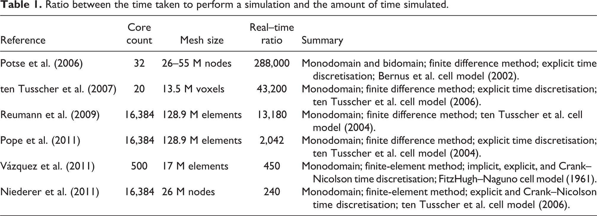
Note that the solvers reported to run efficiently using hundreds of processors or more (i.e. the last four in Table 1) share one or more of the following four limitations: i) they use the monodomain model, ii) they use explicit time discretisations, iii) they use spatial discretisation methods that only allow the use of regular grids (e.g. finite difference method), and/or iv) they are not freely available to the scientific community. This paper focuses on the development of open source cardiac simulation technology that achieves a similar degree of performance in large-scale high-performance computing (HPC) infrastructures using the bidomain equations and a semi-implicit time discretisation on arbitrary spatial domains pathmanathan10. The reasons for these choices are three-fold: several applications of interest (e.g. human shock-induced arrhythmogenesis (Bernabeu et al., 2010b) and drug-induced alterations on the body-surface ECG (Zemzemi et al., 2011)) require the use of the bidomain equations, since the monodomain model presents limitations for their study; explicit time discretisation imposes a constraint on the maximum timestep directly proportional to the grid edge length, so increasing the level of detail of the geometrical models will inevitably lead to increasingly shorter timesteps. This is likely to have a negative impact on overall performance. Unconditionally stable methods (e.g. semi-implicit time discretisation) allow the mesh to become more detailed without requiring shorter timesteps; unstructured grids allow for more realistic representation of ventricular surfaces and fine-grained features than structured grids. The finite-element method is preferred for the spatial discretisation of the bidomain equations for its support of unstructured grids.
This work has been conducted in the framework of the open source Computational Biology simulation package Chaste (Pitt-Francis et al., 2009).
The rest of the paper is structured as follows. Section 2 gives a brief introduction to computational cardiac electrophysiology, including the underlying mathematical models of interest. Section 3 presents the main components of the cardiac electrophysiology solver in Chaste. The parallelisation strategy adopted for each of these components is described in Section 4. Section 5 describes the benchmark used for the evaluation of the scalability improvements presented along with its results. Finally, Section 6 discusses the results and presents the conclusions.
2 Computational cardiac electrophysiology
At a cellular level, models of cardiac electrophysiology of different species and cell types have been successfully developed and used for a variety of applications. The models include representation of the main mechanisms of ionic transport across the cell membrane and between subcellular compartments. From a mathematical point of view, the models typically consist of systems of ordinary differential equations (ODEs), with the most detailed ones (such as Iyer et al. (2007)) having over 60 ODEs. These models allow representation of the effect of mutations, drugs and disease on ion channel function.
At a tissue level, simulating propagation of electrical excitation through cardiac tissue (mainly myocytes) involves solving a system of partial differential equations (PDEs)––the bidomain equations––over an anatomically based computational grid with realistic representation of geometry and microstructure. The level of detail in the models has grown due to a better characterisation of cardiac structure provided by recent advances in medical imaging techniques (Burton et al., 2006). It is now possible to generate highly detailed representations of cardiac structures such as blood vessels, papillary muscles, the Purkinje network and fibre orientation. Preliminary studies have provided insight into the role of previously neglected cardiac structures on ventricular activation following electrical pacing and shocks (Burton et al., 2006). However, this comes at the cost of an increase in problem size and hence computational burden.
2.1 The bidomain equations
For a bidomain simulation of cardiac tissue contained in a conductive surrounding medium, (referred to as the bath) the magnitudes of interest are intracellular and extracellular potentials (


where
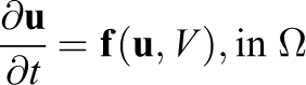
Appropriate boundary conditions are
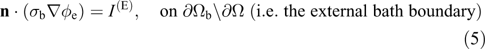
where
Following the spatial discretisation of 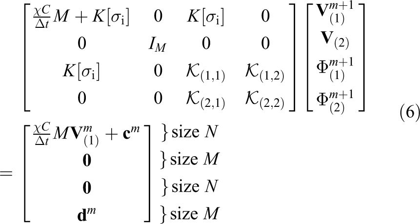
where, at timestep 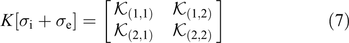
are the appropriate finite-element mass and stiffness matrices and
For simplicity, the linear system in equation (6) can be rewritten as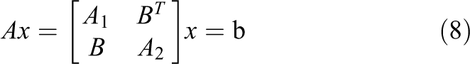
with blocks
2.2 The monodomain model
Under certain circumstances (e.g. see [Keener and Sneyd(1998)]) equations (1)–(3) can be reduced to a PDE of a single unknown, V, coupled to the system of ODEs describing transmembrane ionic transport. The problem to solve, therefore, becomes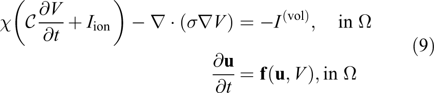
where 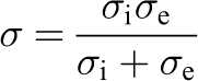
with boundary conditions
This simplification notably reduces the computational burden associated with the numerical solution of the bidomain model. However, it is not suitable for all kinds of application studies. More precisely, More precisely, Potse et al. (2006) concluded that, in the absence of applied currents, propagating action potentials on the scale of a human heart can be studied with a monodomain model. However, note that bath-loading effects are not correctly captured, as discussed in Bishop and Plank (2011).
The final finite-element linear system to be solved for the monodomain model at each timestep can be shown to be: find 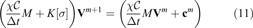
3 Large-scale cardiac electrophysiology simulation with Chaste
Chaste is an open source computational framework for the simulation of systems in biology, with a particular focus on cardiac electrophysiology, cancer modelling, and tissue growth. It aims to be extensible, robust, fast, accurate, maintainable and to use state-of-the-art numerical techniques, is distributed under the LGPL and BSD licenses and can be downloaded from www.cs.ox.ac.uk/chaste. For a detailed description of the Chaste project, its aims and functionality, the reader can refer to Pitt-Francis et al. (2009).
3.1 Main components of Chaste’s cardiac electrophysiology solver
Running a cardiac electrophysiology simulation consists of a number of different stages, illustrated in Figure 1. In the first phase of the simulation, the simulation parameters (including simulation duration, timesteps, tolerances, cell models etc.) are defined, the mesh is loaded from file, initial and boundary conditions are specified and the matrix defined in equations (6) or (11) is assembled. Subsequently, at each timestep, individual cell models at each mesh node are integrated (ODE solution), the right-hand-side vector in equations (6) or (11) is assembled and then the resulting linear system is solved. It should be noted at this point that although Figure 1 illustrates the stages of a cardiac electrophysiology simulation code, there are aspects of the problem which are generic to FEM programming in general. Nevertheless, some differences may occur: e.g. many FEM solvers do not need an ODE solver stage, problems with a time-varying left-hand side would require the “Assemble matrix” component to be inside the time-loop rather than in the initial phase, non-linear PDE solvers would require the linear system stage to be inside another iterative loop, and static problems like stress analysis would need no time loop. In the following sections (as annotated in Figure 1) the schemes implemented for reducing the parallel scaling bottlenecks in the Chaste code are described.
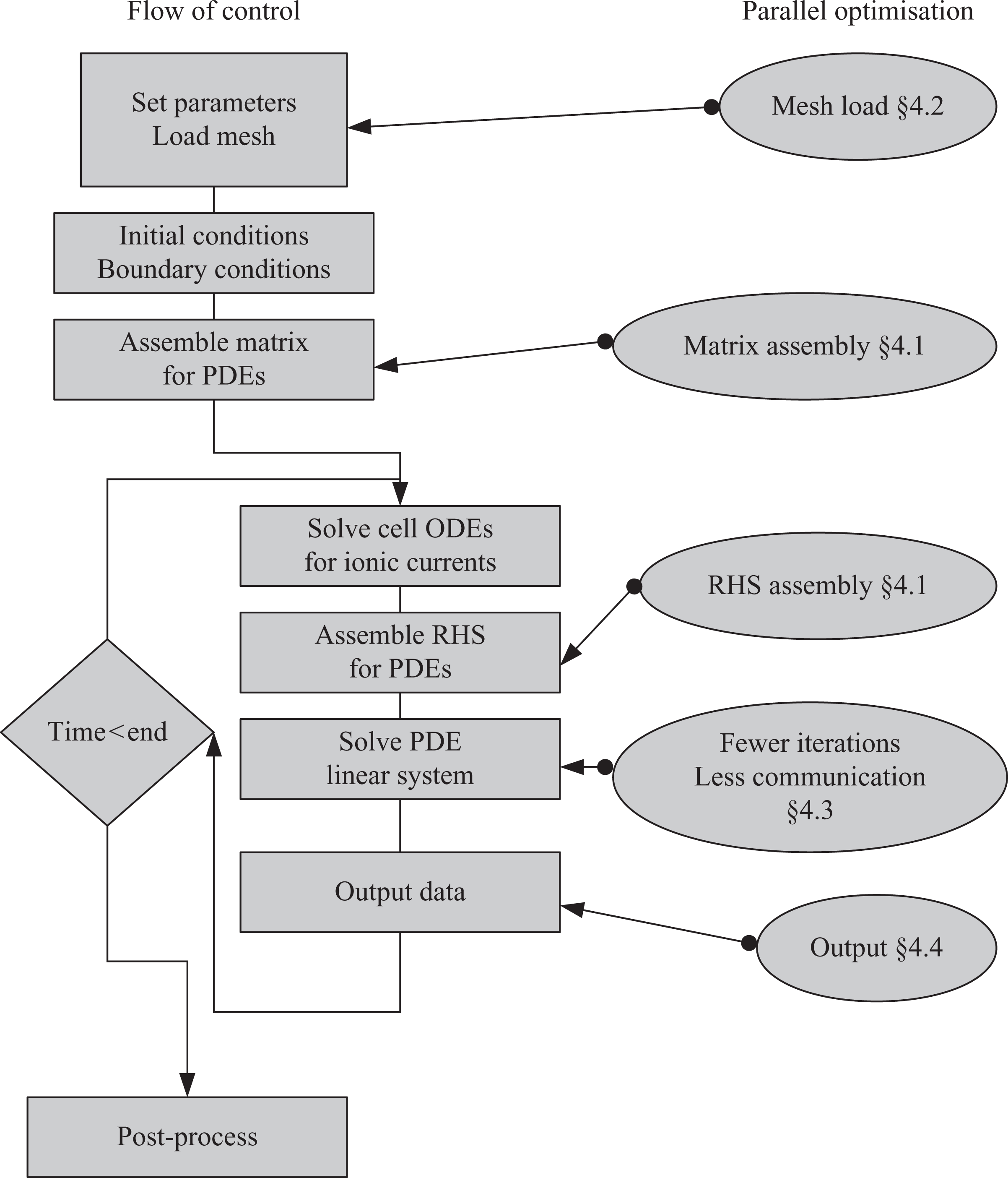
A schematic of the main components of the solver with cross-references to the sections describing parallel improvements made during this study.
3.2 Initial performance evaluation
In order to evaluate the performance of Chaste on large-scale supercomputers with realistic 3D cardiac models, an electrical propagation benchmark using a 4 million node anatomically-based rabbit ventricular mesh (Bishop et al., 2009) was designed. The benchmark consists of an apical stimulus followed by simulation of 100 ms of bidomain activity in the cardiac tissue only (i.e. there is no bath). The choice of 100 ms as total simulation time is a compromise between: i) simulating for a period of time that is short enough to be tractable with the lowest core count considered (i.e. 32 cores); and ii) choosing a simulation time that is representative of our applications of interest (e.g. hundreds of ms in Bernabeu et al. (2010b) and Zemzemi et al. (2011)). Table 2 summarises the experimental details.
Benchmark configuration.
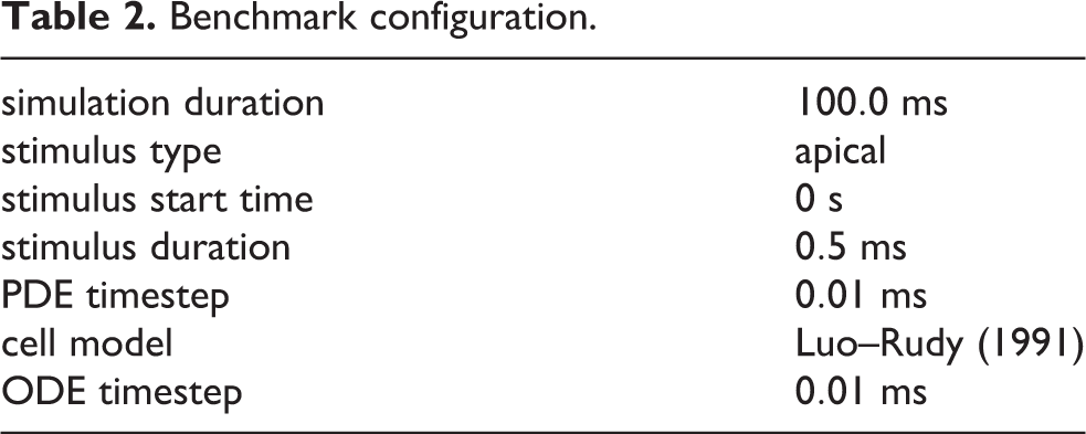
The following parameters were used in equations (1)–(5):
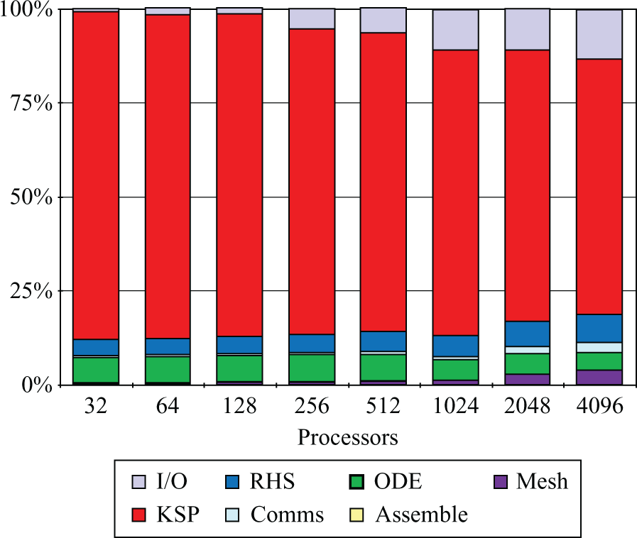
Prior to making any performance improvements, the benchmark was run on Phase 2a of the HECToR supercomputer, a Cray XT4 system with 3072 compute nodes (at the time of the study). Each compute node consisted of an AMD 2.3 GHz Opteron Barcelona quad-core and each quad-core socket shared 8 GB of memory and a Cray SeaStar2 chip router with 6 links used to implement a 3D-torus network topology. Figure 2 presents, for an increasing number of cores, the proportion of time spent by the benchmark simulation in each of the stages described in Section 3.1.
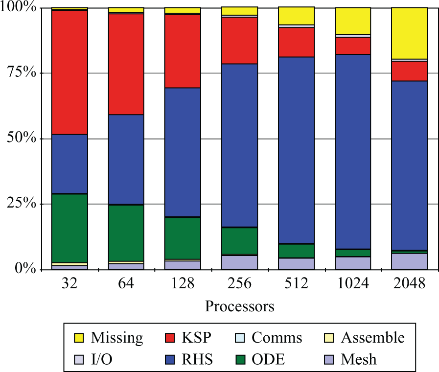
Original time breakdown before the improvements presented in this paper.
The first thing to note is that, as core count increases, the time within the ‘Missing’ section starts to increase. Further profiling confirmed that it was spent outside the main stages cited earlier and therefore it was potentially redundant. More precisely, it was identified to be unnecessary synchronisation and disk access contention when writing Chaste’s log files. Interestingly, this performance degradation had passed previously unnoticed when running in small size clusters and workstations (note how it is hardly visible for
It is also clear from Figure 2 that the proportion of time spent in ‘RHS assembly’ increases with core count and starts to dominate the total execution time for p > 128. This is a good indicator of poor scaling and therefore it was one of the first issues addressed (Section 4.1.2). It can also be seen that the time spent in ‘Mesh load’ also scaled poorly. There are two reasons for this: the sequential nature of the algorithm used for domain decomposition (METIS) and disk access contention. Section 4.2 describes how these two issues were addressed.
The two stages taking most of the time at p = 32 (i.e. ‘System solution’, labelled as KSP, and ‘ODE solve’) do not show major scaling problems or, where they do, it is not as severe as those seen with ‘RHS assembly’ or ‘Mesh load’. For ‘ODE solve’, this is expected behaviour since the problem is embarrassingly parallel, so will scale linearly provided that an even distribution of the ionic models among the available processors is generated. This part of the code has also been tuned (see Cooper (2009)) in order to reduce ODE solution time, but this tuning has had no impact on overall parallel efficiency. In contrast, ‘System solution’ involves the use of tightly coupled parallel algorithms that are likely to scale suboptimally. Following the improvements introduced in the ‘Missing’, ‘RHS assembly’, and ‘Mesh load’ stages, the analysis presented in Figure 2 was repeated, showing ‘System solution’ as the next target for improvement (results not shown here). The proposed improvements are summarised in Section 4.3.
Finally, it is noted that most of the initial phases of the solver (such as the application of boundary conditions or the assembly of the system matrix) do not have a major impact in parallel scalability. The post-processing phase (which essentially involves converting data formats for visualisation and analysing data) is application-specific and was outside the scope of this publication.
4 Parallelisation
4.1 Linear system assembly
When solving systems of coupled PDEs with FEM, several fields are computed at each discretisation point (two in the case of the bidomain equations). In this context, a design decision has to be taken regarding how unknowns are arranged in the linear system. The options are to use either a ‘blocked’ distribution (i.e.
Another relevant design decision concerns the way that the computational domain is partitioned. In principle, it is possible to partition either node- or element-wise. This decision has important consequences in terms of load balancing. The initial performance evaluation in Section 3.2 showed that the linear system and ODE solution stages dominate total execution time for low core counts. In both cases, execution time at each subdomain is a function of the number of grid points assigned (i.e. number of degrees of freedom and number of cell models, respectively). Therefore, it makes sense to partition node-wise to ensure that the number of grid points in each subdomain stays as constant as possible. Partitioning element-wise would instead optimise the element distribution (which would have a positive impact on stages like matrix assembly). Unfortunately, it would potentially generate a suboptimal node distribution and therefore unbalance the stages that dominate total execution time.
Hence, mesh elements need to be distributed among the available processors based on node ownership. For elements located at the border between two partitions (like II and III in Figure 3) a strategy for ownership assignment is required. Some options are: i) assigning each of them to the processor owning the larger number of nodes within the element, ii) allowing multiple ownership of an element or iii) distributing them in such a way that the number of elements owned by each processor is balanced. Some of the implications of this choice are discussed later in this section.
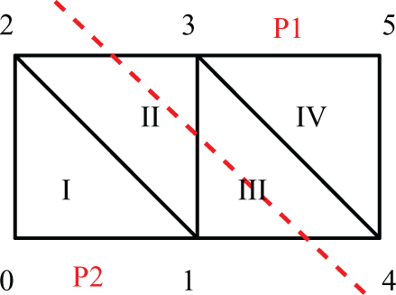
Model problem geometry. Dashed line shows parallel partition.
4.1.1 Matrix assembly
A commonly used method to assemble matrix 
that is the Boolean matrix that maps 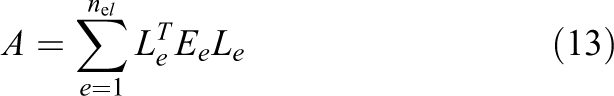
where the effect of pre- and post-multiplying
In a parallel simulation, the
More formally, let 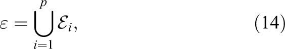
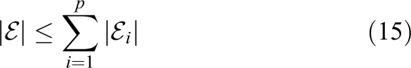
and consider a row-based distribution of the system matrix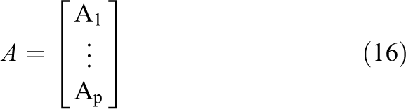
where 
be the Boolean matrix that maps 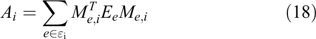
if and only if i) an interleaved ordering of unknowns and ii) multiple ownership of elements are implemented.
These two design decisions imply that for an element
4.1.2 Right-hand side assembly
In Chaste’s original design, vector 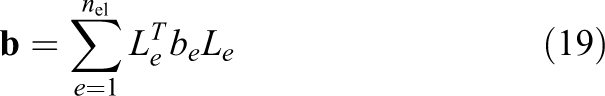
where
It was shown in Pathmanathan et al. (2010) that, provided 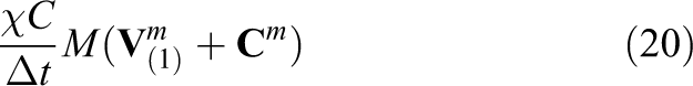
where
One final consideration is that in the case of bidomain RHS assembly, equation (20) only accounts for the first 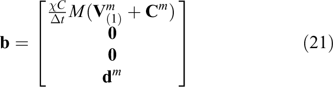
and a data partition compatible with equation (16)
with
Finally, evaluating
4.1.3 Implementation details
Chaste uses PETSc parallel data structures (Balay et al., 2010) wherever possible. When constructing parallel matrices, PETSc allows for data to be generated non-locally. At the last stage of construction (known as assembly), PETSc will work out the appropriate owner and migrate the data. This process requires several rounds of parallel reductions in order to ensure consistency among all the processes, even when no data is being migrated. It is possible to disable this check provided that all the data is generated locally, reducing the number of parallel reductions required with an important impact in parallel scalability. In PETSc version 3.0 this can be done for matrices with the following function call:
4.2 Mesh load and partitioning
The first step in running a simulation is to read in the mesh representing the system geometry from a file. In a parallel simulation it is then also necessary to partition this mesh between the available processes. In general, this one-time cost is relatively low for a sequential simulation––and, hence, little consideration has been given to optimising it.
At the beginning of this work, Chaste used the METIS-based mesh partitioning algorithm described in Pathmanathan et al. (2010). This method requires each process to perform a sequential partition of the mesh in order to determine which nodes it owns. This makes METIS unsuitable for partitioning meshes that are too large to fit into memory on a single core. Further, since each process calls METIS sequentially and the temporal cost of the partitioning algorithm is a function of the number of partitions, the overall time to obtain the partition increases (even for a fixed mesh) with the number of processes. Hence, for HPC simulations, Amdahl’s law (Amdahl, 1967) means that the cost of loading the mesh rapidly increases relative to all other parts of the code (the work for which can be distributed). Modifying the algorithm to use ParMETIS (Schloegel et al., 2002), the parallel version of METIS, is relatively straightforward (in Chaste, ParMETIS is instead accessed via PETSc wrapper functions that provide the functionality required to partition based on nodes that is absent when calling ParMETIS directly).
A good mesh partitioning will not only balance the amount of geometry on each compute node (and thus balance the work load), but will also minimise the communication boundaries and reduce the skyline of the main matrix. The effect of the mesh partition on the matrix structure results in improvements to the matrix assembly (Section 4.1.1), to the RHS assembly (Section 4.1.2) and the system solution (Section 4.3). We have previously quantified these improvements in Pathmanathan et al. (2010).
The importance of the mesh partitioning step has been previously acknowledged in the literature (e.g. see Devine et al. (2005) and Teresco et al. (2006)). Furthermore, it has become of increasing interest due to the substantial increment in the number of cores available in emerging architectures (Devine et al., 2006; Zhou et al., 2012). In particular, the use of ParMETIS-based partitioning algorithms for parallel finite-element method simulations has been widely reported in the literature (Piggott et al., 2008; Sahni et al., 2009; Bekas et al., 2010; Shadid et al., 2010; Niederer et al., 2011). In the current section, we also consider an often neglected aspect of the problem: the design of a scalable algorithm that, given a ParMETIS partition, reads the mesh from disk and creates the relevant data structures.
The original file format used in Chaste to represent meshes consisted of separate ASCII files containing
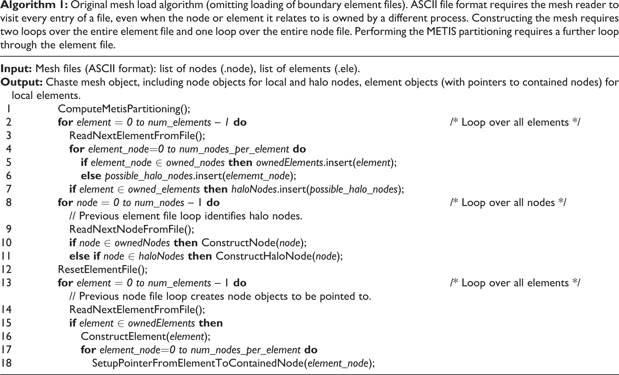
lists of node coordinates (.node file), a list of the nodes contained in each element (.ele file) and a list of the nodes contained in each surface element (.face file). For large meshes these files can grow to be very large, e.g. for a mesh containing approximately 4 million nodes and 24 million elements the file sizes are 129 MB (node), 958 MB (element) and 33 MB (face). Further, non-constant field length in ASCII files makes it difficult to implement random access, so it is necessary for each process to read the three files in their entirety, determine what information it needs to retain and discard the rest. In practice––since the software must be able to deal with files that are too large to fit in the memory available to a single process––the element file must be read several times, as can be seen in Algorithm 1, which shows the initial Chaste mesh load algorithm (excluding the face file read, which is equivalent to the final element file read).
Original mesh load algorithm (omitting loading of boundary element files). ASCII file format requires the mesh reader to visit every entry of a file, even when the node or element it relates to is owned by a different process. Constructing the mesh requires two loops over the entire element file and one loop over the entire node file. Performing the METIS partitioning requires a further loop through the element file.
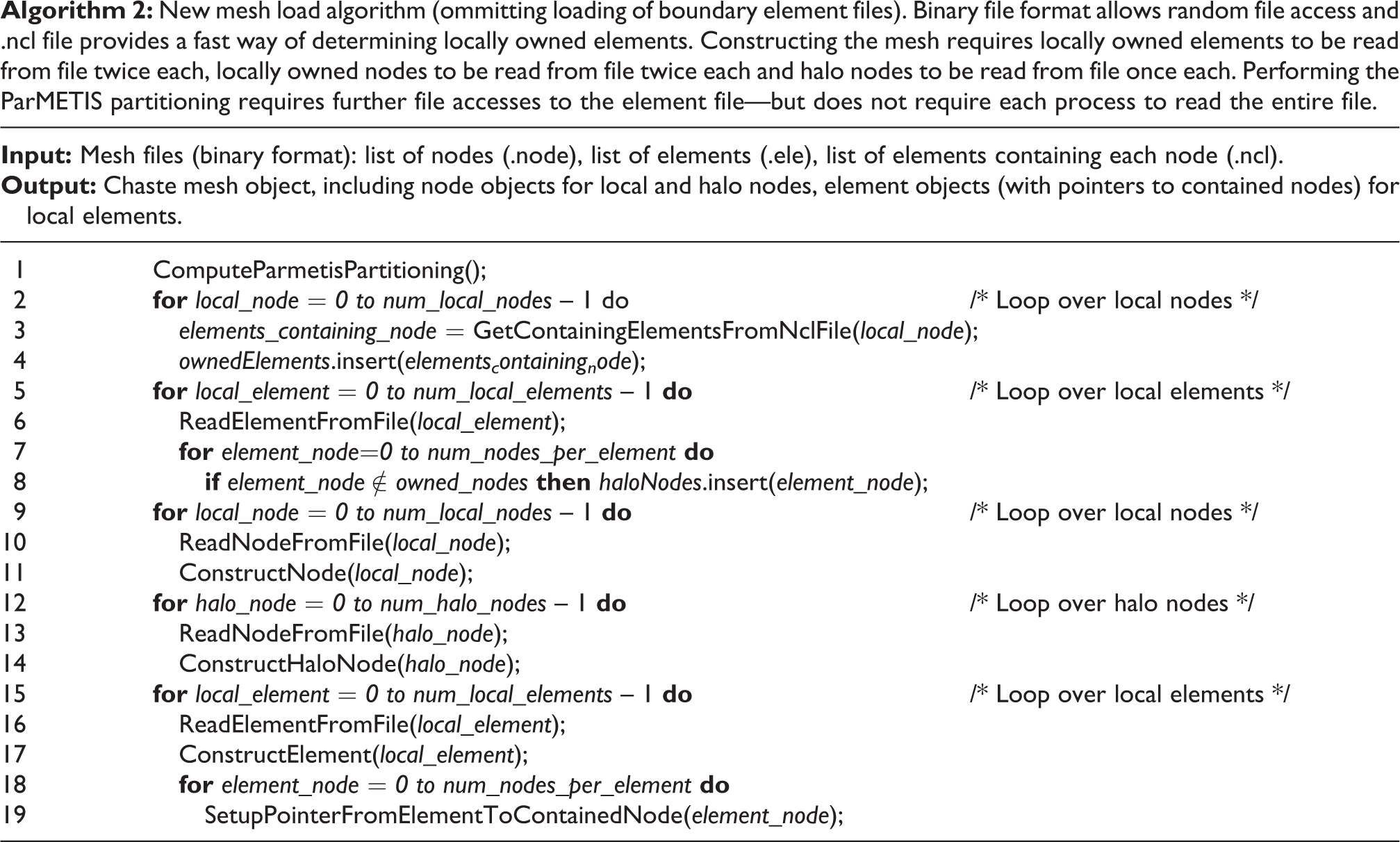
In order to reduce the amount of data that each process was required to read, the files were converted to binary format. This has two consequences: the files are smaller (and hence can be read in less time) and each entry is a fixed size (allowing random access, meaning that each process can jump straight to the entries it needs to read). However, since a process owns an element if it also owns one or more of its nodes, it is necessary for that process to interrogate each element in turn to determine whether or not it owns it––and (as seen in the first loop over elements in Algorithm 1) this necessitates a complete pass through the element file (generally the largest of the mesh files). Even when using a binary file format this is expensive and does not scale in parallel. Thus, a fourth (binary) mesh file was introduced for the largest meshes. This is the reverse of the element file: containing a list of which elements each node is contained in (known as the node-connectivity list or .ncl file). Each process can then access the parts of the .ncl file that correspond to the nodes that it owns and very rapidly construct a list of the elements that it owns. The process is then able to access directly only the parts of the element file that it needs to. Note that for a simulation on
New mesh load algorithm (ommitting loading of boundary element files). Binary file format allows random file access and .ncl file provides a fast way of determining locally owned elements. Constructing the mesh requires locally owned elements to be read from file twice each, locally owned nodes to be read from file twice each and halo nodes to be read from file once each. Performing the ParMETIS partitioning requires further file accesses to the element file—but does not require each process to read the entire file.
The improvements presented in this section only refer to algorithmic problem considerations, that is, ensuring that the volume of data read by each process decreases with the number of processes involved (for a fixed problem size). The authors believe that the techniques presented are generic enough to be usable by other parallel finite-element codes. However, we also acknowledge that achieving a good interaction with the underlying parallel file system will greatly influence the algorithm implementation performance. Such a task requires substantial knowledge of the underlying parallel file system and architecture and is beyond the scope of this work.
4.3 Linear system solution
Most authors choose the conjugate gradient (CG) algorithm for the solution of mono/bidomain FEM linear systems (e.g. Colli-Franzone and Pavarino (2004), Plank et al. (2007), Pennacchio and Simoncini (2009) and Pathmanathan et al. (2010)). However, other Krylov subspace methods such as GMRES (e.g. Whiteley (2006)) or Bi-CGSTAB (e.g. Potse et al. (2006)) have been successfully applied as well. In order to study the parallel efficiency of different iterative solvers, the different computational kernels involved must be considered individually. In the case of Krylov subspace methods, these are: i) vector inner products, ii) vector–vector linear combination (axpy) operations, iii) matrix–vector products, and iv) preconditioner application. axpy operations do not compromise parallel scalability since they can be performed without need of communication (assuming a consistent parallel distribution of all the vectors involved). Matrix–vector products require a certain degree of communication, but, as shown in Pathmanathan et al. (2010), reduction of the matrix bandwidth through the use of graph-based domain decomposition techniques increases scalability. The scalability of the preconditioning step is determined by the preconditioning technique of choice: preconditioners such as point Jacobi or block Jacobi with incomplete factorisation at each subblock do not require communications. Whole matrix incomplete factorisation or multigrid techniques are tightly coupled algorithms that require a higher degree of communication. Finally, vector inner products are communication-intensive operations as they are often implemented as parallel reductions. Parallel reductions are also required when checking for convergence if the stop criteria are based on the evolution of the
4.3.1 Inner product reduction
Several authors (e.g. Barrett et al. (1994) and Gutknecht and Röllin (2002)) have proposed the use of the Chebyshev Iteration (CI) method (Golub and Van Loan, 1996) for the solution of the symmetric linear systems
hence avoiding inner products which often become a performance bottleneck in parallel hardware. The method requires enough knowledge about the spectrum of the preconditioned operator 
with 
where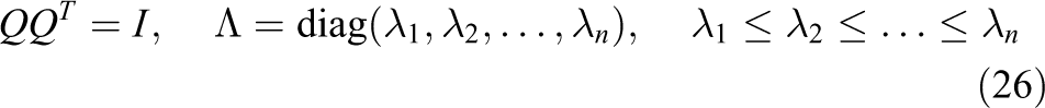
the method requires knowledge about the interval 
With this information, the method defines a family of Chebyshev polynomials
The following result will be useful in later discussion: let 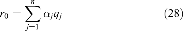
Then, it can be shown (e.g. see Calvetti et al. (1994)) that
Based on a survey of the literature, it appears that the CI method has never been successfully applied to the solution of the mono/bidomain equations using modern parallel hardware. Two possible reasons for this are: i) the intrinsic difficulty of estimating
In Calvetti and Reichel (1996) a hybrid iterative method that alternates CG and Richardson iterations for the solution of symmetric positive definite linear systems is proposed. The method starts by performing 
(with associated eigenvectors 
The Richardson iteration is then resumed with the new interval. The hybrid scheme alternates between CG and Richardson iterations as described until a sufficiently converged solution of equation (23) is found. Note that the definition of
In the current work, this idea is extended to the solution of linear systems with multiple—but not simultaneously available—right-hand sides, as is the case in the FEM solution of the mono/bidomain equations and other systems of PDEs including time derivatives. Interleaving complete CG and CI solves is proposed, rather than interleaving CG and Richardson iterations within the same solve. This is motivated by the fact that efficient parallel implementations of CG and CI solvers are readily available and can be used as black boxes. In this case, CG is used both for solving the first timestep (and possibly later ones) and for computing (via the aforementioned Lanczos connection) the interval
Solution residual
The choice of
Number of iterations taken by CI initialised with
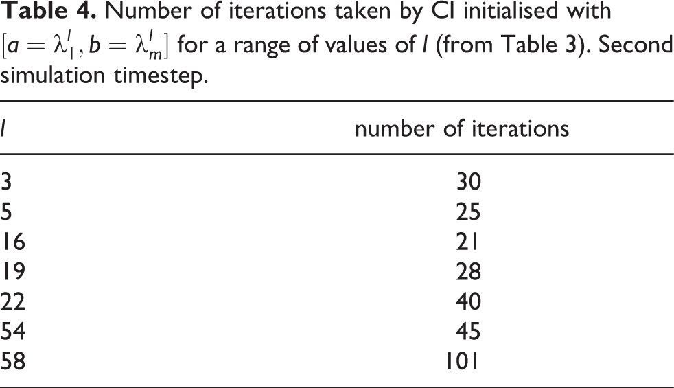
It can be observed that the minimum number of iterations is achieved with
Finally, it cannot be expected that the choice of parameters
4.3.2 -Norm reduction
Even in the cases when an inner-product free iterative method (such as CI) is used, one global reduction per iteration is required when the stop criteria of the method is based on the evolution of the
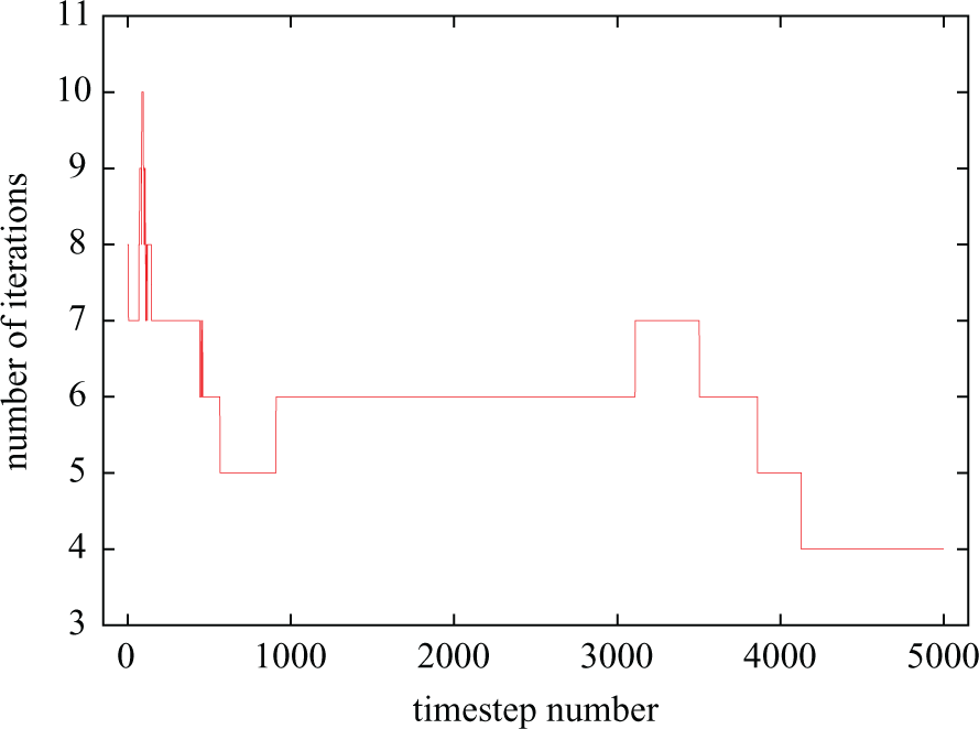
Number of iterations taken by CI (
Sudden changes in iteration count are triggered by events such as stimuli application (both user-defined and coming from self-stimulating cells), the presence in the domain of polarisation/repolarisation wavefronts and, in general, any event inducing sudden changes in
4.3.3 A hybrid CG–Chebyshev method
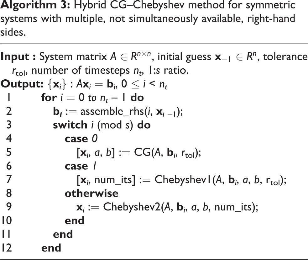
Algorithm 4.3.3 summarises the techniques presented in Sections 4.3.1 and 4.3.2 for the reduction of inner products and
Hybrid CG–Chebyshev method for symmetric systems with multiple, not simultaneously available, right-hand sides.
In order to evaluate the error introduced by the use of a fixed number of iterations, a benchmark consisting of 500 ms of bidomain activity following an apical stimulus on the UCSD rabbit model (Vetter and McCulloch, 1998) was designed. Figure 5(a) plots the infinity norm of the error against time for a range of values of 1 :
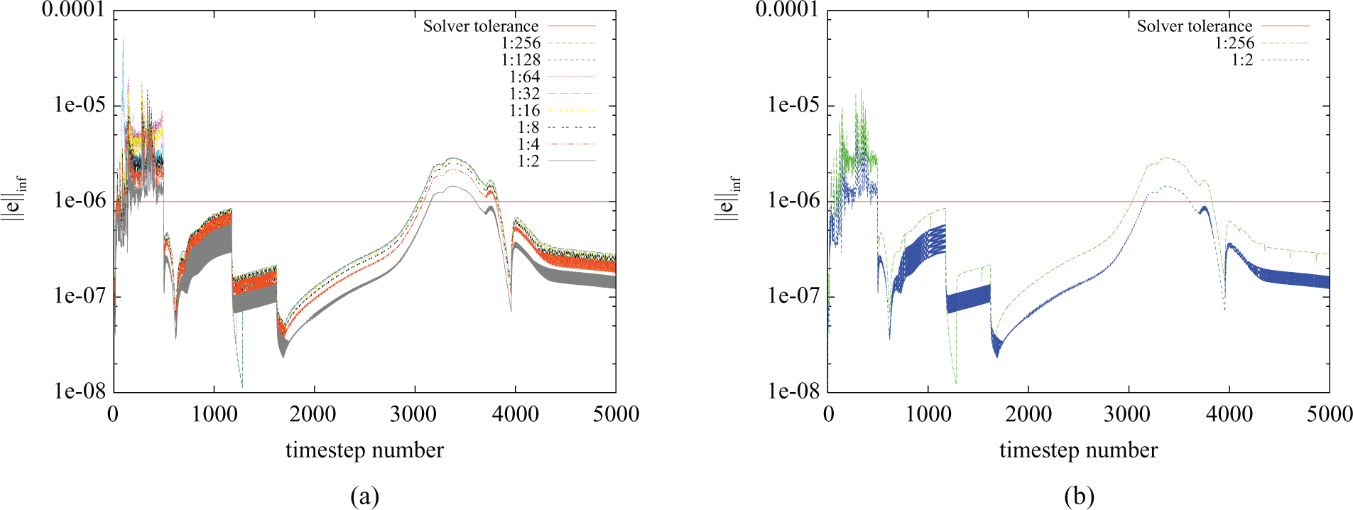
Error introduced by several configurations of the ratio 1 :
4.3.4 Preconditioning
Bidomain preconditioning has become an active field of research over the past years (dos Santos et al., 2004; Pennacchio and Simoncini, 2009; Plank et al., 2007; Pavarino and Scacchi, 2008). Algebraic multi-grid (AMG) preconditioning has been successfully applied to the efficient solution of bidomain linear systems. However AMG does not exhibit mesh-independent convergence properties, i.e. the convergence rate of an AMG-preconditioned linear solver will deteriorate with refinement of the computational domain. In order to address this issue, mesh-independent bidomain preconditioners have been proposed (Pennacchio and Simoncini, 2009; Bernabeu et al., 2010a). In Bernabeu et al. (2010a), we propose a preconditioner that exploits the block structure of the matrix in order to reduce computation time and achieve mesh-independent convergence. In a more recent publication (Bernabeu and Kay, 2011), we present scalable parallel implementations of the techniques described in Bernabeu et al. (2010a) and identify a dependency of the most efficient bidomain preconditioner on the coefficient between the PDE solution timestep and the square of the spatial discretisation (
4.4 Output
Output of the results of a massively parallel simulation is not as straightforward as in the sequential case or for a small number of processes. In these cases periodically writing the values of the variables of interest to a single file is likely to be relatively cheap compared to the cost of computing the solution. However, this strategy does not scale as the number of processes increases: each process in turn has to open the file, write its data and then close the file—and, hence, the time required to do this increases for a larger number of processes. This problem can be compounded if the computational resource being used has a distributed file system (e.g. Lustre or NFS), requiring additional time to be spent communicating the data to the location at which it is to be stored. So, small tasks (such as updating a file that tracks the progress of the simulation) that can be completed in a very small time by each process, and barely show up in profiling in parallel, even when using 10 s of processes can become very severe bottlenecks at larger scales as processes compete to write to disk. Hence, where possible, global information should be calculated and written to file by a single process (without communication) even though this may lead to other processes remaining idle and may result in less readable code.
However, for output of the simulation’s variables (which are distributed over all processes), bandwidth limitations mean that it is not efficient to concentrate data on a single process for output. Hence, Chaste was designed to make use of the HDF5 parallel I/O library (http://www.hdfgroup.org/HDF5). Based on MPI-IO, this provides a set of routines that efficiently write complex data structures to disk in parallel. The results of this have proved to be mixed: while the use of HDF5 does seem to prevent the time required to perform I/O from increasing significantly as the number of processes increases, the code does not appear to scale in parallel when used within Chaste and timings (on any number of processes) are extremely inconsistent.
5 Results
Following the initial performance evaluation presented in Section 3.2 and the description of the proposed improvements in Section 4, we now turn our attention to the evaluation of those improvements.
5.1 Scalability improvements
5.1.1 Mesh load
Figure 6 shows the time taken by the mesh-load stage against the number of cores for five different versions of the code. In the original version, the mesh-load time increased rather than decreased with the number of processors. There were two reasons for this: i) mesh files were read in their entirety by all the processors and ii) a sequential algorithm was used to compute the partitions. In this scenario, mesh-load time will, at best, remain constant. However, the fact that all the processors were concurrently accessing the entire set of files produced disk access contention due to the large number of read operations issued at large core counts. Further, in the case of ii) the asymptotic cost of the algorithm is directly proportional to the number of partitions to be generated (i.e. to the number of processors running the simulation).
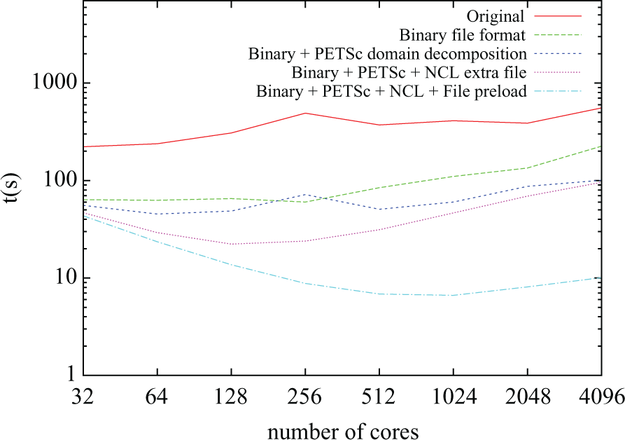
Mesh load time for different numbers of cores.
Following the introduction of a binary file format, mesh-read times were reduced by a factor of 4.21 on average, mainly due the fact that data representation was more compact and direct access could be performed on the node file. However, scalability still remained an issue. Next, the addition of PETSc-based partitioning (instead of raw calls to METIS) allowed for the partitioning step to be performed in parallel, greatly reducing the execution time for large core counts: a factor of 2.23 for
In the final version of the code (labelled “Binary + PETSc + NCL + File preload” in Figure 6) a warm-up run is performed before the actual simulation being timed in order to validate the hypothesis about the file access contention. The rationale behind this is that the files will be cached by the distributed file system before the time the second run starts, therefore reducing latency and hiding disk access contention. When compared with the previous version, it can be seen that the mesh-load time stays fairly constant for
5.1.2 Right-hand side assembly
The time taken by the RHS assembly stage is plotted against number of cores for three different versions of the code in Figure 7. In the original implementation, it can be seen that execution time remained constant no matter how many cores were used. Recall that this problem had been identified in Figure 2. The poor scaling resulted from the distributed vector containing the solution at the previous timestep (
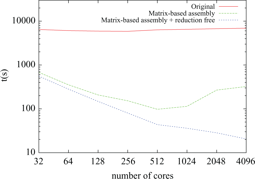
Right-hand side assembly time for different numbers of cores.
Even for low core counts, the original implementation turned out to be one order of magnitude slower than later improvements. The first of these improvements (plotted as “Matrix-based assembly” in Figure 7) comes from the elimination of global gather operations and from the switch from element-wise assembly to matrix-based assembly described in Section 4.1.2. It can be seen that the solution scales well for up to 512 cores; however for larger core counts, the execution time increases. Further profiling showed that this was due to the increasing time spent performing parallel reductions during the assembly of
5.1.3 System solution
At the beginning of this work, CG was Chaste’s default linear solver. However, when the code was ported to HECToR other available linear solvers were evaluated. It was found that PETSc’s implementation of the SYMMLQ algorithm was competitive. Finally, the hybrid CG–Chebyshev algorithm presented in Section 4.3 was also successfully ported.
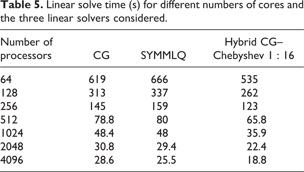
Table 5 shows the time taken by the system solution stage against the number of cores for the three linear solvers mentioned. It can be seen that the SYMMLQ algorithm is faster than CG for 1024 or more cores. This was unexpected since SYMMLQ needs to perform extra work to overcome the potential indefiniteness of the linear system. The magnitude of the difference in time suggests that this speedup is most likely to be due to implementation characteristics. Further profiling needs to be performed in order to validate this hypothesis. The hybrid CG–Chebyshev method is faster than any of the previous methods for all the core counts considered. For
Linear solve time (s) for different numbers of cores and the three linear solvers considered.
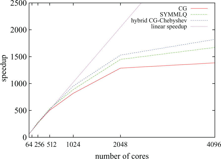
Parallel speedup for the three linear solvers considered and an increasing number of processors.
5.2 Final time breakdown
Following optimisation, the proportion of time spent by the benchmark simulation in each of the stages described in Section 3.1 is shown, for a range of processor counts, in Figure 9. This figure is exactly equivalent to the analysis before optimisation shown in Figure 2.
Final time breakdown after the improvements presented in this paper.
Firstly, note that the time initially reported as ‘Missing’ has been successfully removed. Secondly, the ‘RHS assembly’ stage has been greatly improved: it now takes no more than 8.6% of the total execution time (against 25–65% in the original time breakdown) and also scales almost linearly up to 1024 cores, degrading only slightly for 2048 and 4096 cores. Thirdly, the proportion of time spent reading in the mesh has been greatly improved, being almost unnoticeable for 32–1024 cores. However, the increasing proportion of time spent for 2048 and 4096 cores highlights the fact that the absolute time spent in this stage is actually higher than for 1024, indicating that the execution is probably suffering from file access contention. Nevertheless, the ‘Mesh’ time for
Finally, two operations that were almost unnoticeable in the initial time breakdown increase their presence at large core counts: ‘I/O’ and ‘Comms’ (which cover writing out the simulation results and performing certain synchronisations and distributed error checks). There are two reasons for this: i) both operations involve either synchronisation or access to resources with a low degree of replication (such as Lustre I/O nodes), and ii) the benchmark used consists of around 8 million degrees of freedom, at
6 Discussion and conclusions
In this paper, effective parallelisation strategies for Chaste’s bidomain solver have been described. The code was initially ported to HECToR (the UK’s high-end computational resource), where simulations could be run using two orders of magnitude more processors than ever before. Initial profiling highlighted a number of scalability issues only identifiable at a large scale (e.g. mesh read, RHS assembly, linear system solution). Section 4 describes the techniques implemented to address these issues, including novel computational and numerical techniques as well as techniques at the interface between them. Of particular interest is the novel hybrid CG–Chebyshev linear solver presented in Section 4.3. Although the hybrid concept was first introduced in the late 1980s, a literature survey indicates that the Chebyshev Iteration method has not been successfully applied to the reduction of linear system solution time using modern parallel hardware.
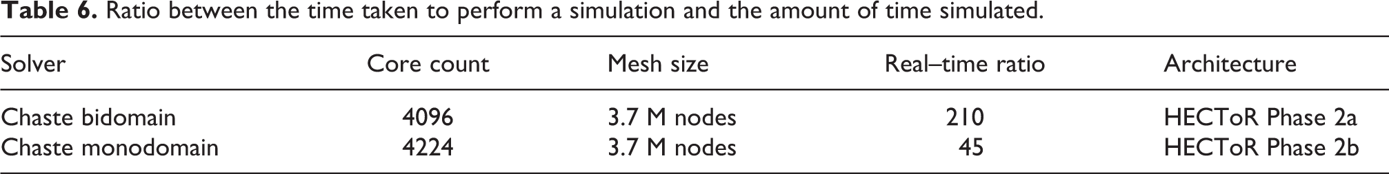
Figure 10 compares parallel speedup before and after the work presented in Section 4. It can be seem that in the code described in Section 3.2 (solid red line), speedup saturated at around 100 no matter the number of processors used. The optimisations allowed for speedups of over 1400 (compared to sequential execution) and resulted in optimal or near-optimal scalability for up to 512 cores. They yield a combined improvement (compared to the initial code) by a factor of over 140 in the fastest possible execution time for the benchmark, meaning that Chaste’s bidomain solver is now two orders of magnitude faster than at the beginning of the work described here. Further optimisations relating to sequential performance (with no impact on parallel scaling) have also been described in Southern et al. (2011). Table 6 summarises the real–time ratios achieved as a result of all the optimisations. The values represent an improvement with respect to those in Table 1. One limitation of our work is that scalability is only examined under sinus rhythm propagation and not during reentry. During reentry multiple wavefronts coexist and interact in the domain. How this affects load balancing and scalability needs to be determined.
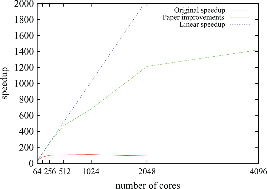
Chaste’s scalability for a typical bidomain simulation before (solid red line) and after (broken green line) the improvements presented in Section 4.
Ratio between the time taken to perform a simulation and the amount of time simulated.
It can, therefore, be concluded that this work has brought Chaste to the level of parallel performance necessary to run simulation studies with state-of-the-art whole-organ geometrical models (including human ventricular models). As a result of the improvements described here, it has been possible to conduct further studies (Bernabeu et al., 2008, 2009; Zemzemi et al., 2011) that would otherwise have been impossible due to the prohibitive computational expense required. Furthermore, given that Chaste is one of the first open source software platforms for bidomain simulation, the improvements are likely to have an immediate impact in the community, by making large-scale computational cardiac electrophysiology simulation more accessible, thus avoiding the overhead of developing multiple, often repetitive, in-house codes.
Footnotes
Acknowledgements
The authors would like to thank Dr Martin Bishop for providing some of the geometries used in this study, HECToR’s helpdesk, and the Chaste development team (http://www.cs.ox.ac.uk/chaste/theteam.html).
Funding
The work of Miguel O Bernabeu, James Southern, Nicholas Wilson, Jonathan Cooper and Joe Pitt-Francis, part of the preDiCT project, was supported (entirely or partially) by a grant from the European Commission Directorate General for the Information Society (grant number 224381). The work of Jonathan Cooper was also partially supported by the European Commission under the VPH NoE project (grant number 223920).