Sage Journals: Discover world-class research

Abstract

Allometric scaling between metabolic rate, size, body temperature, and other biological traits has found broad applications in ecology, physiology, and particularly in toxicology and pharmacology. Basal metabolic rate (BMR) was observed to scale with body size and temperature. However, the mass scaling exponent was increasingly debated whether it should be 2/3, 3/4, or neither, and scaling with body temperature also attracted recent attention. Based on thermodynamic principles, this work reports 2 new scaling relationships between BMR, size, temperature, and biological time. Good correlations were found with the new scaling relationships, and no universal scaling exponent can be obtained. The new scaling relationships were successfully validated with external toxicological and pharmacological studies. Results also demonstrated that individual extrapolation models can be built to obtain scaling exponent specific to the interested group, which can be practically applied for dose and toxicity extrapolations.

Keywords

allometric scaling metabolic rate extrapolation dose toxicity

Introduction

Metabolism supports life and relates to many important biological traits. Despite the size of organisms spans over 21 orders of magnitude,¹ basal metabolic rate (BMR) relates to body mass (M) by a simple power function of BMR = aM^b (refer to the first scaling relationship).^2

–9 This scaling relationship has been broadly used by toxicologists for toxicity and dose extrapolations, a typical example is the calculation of human equivalent dose (HED) from animal dose.^10

–15

Since the 1830s, the scaling exponent has been debated on whether it should be 2/3, 3/4, or neither.^4,16

-21 As a result, exponents of 1/3 and 1/4 were both widely used in toxicity extrapolations.^{3,10,11,14,15} The 3/4 exponent gained support thanks to the West, Brown, and Enquist (WBE) vascular resource supply network model, or WBE model²² and metabolic theory of ecology (MTE) developed over a decade ago,²³ which is described by MR = aM ^3/4 e^−E ^/(kT), where E is activation energy, k is the Boltzmann constant, and T is body temperature. However, the MTE model and its derivation of the 3/4 exponent have been increasingly questioned on many aspects such as its 8 assumptions, the limit of infinite network size, and the sensitivity of the exponent to the variations in the assumptions.^24

-31

Stumpf and Porter³² pointed out that a robust scaling power law should encompass mechanistic, statistical, and empirical support, and apparently current models lack such robustness. In an effort to better characterize the relationships between BMR, body mass, body temperature, and biological time, 2 new scaling relationships were derived based on thermodynamic principles. Linear regressions were conducted between these 4 biological traits with empirical data, and applications to dose and toxicity extrapolation from animals to humans were also discussed.

Methods

Thermodynamic Basis

Two major sources of energy gained by an organism are biochemical energy stored in food and light energy from solar radiation. At basal metabolic conditions, the gained energy is mainly used to support various metabolic processes or partly accumulated as body material:

M_{f o o d} + E_{l i g h t} = B M R + M_{a c c}

where M _food is food consumed, E _light is the absorbed light energy, and M _acc is body material accumulation.

Metabolic energy eventually dissipates into the environment as various forms of heat as shown in Figure 1:

B M R = Q_{r} + Q_{c o n v} + Q_{c o n d} + Q_{H_{2} O} + Q_{w} + Q_{o t h e r}

Figure 1.

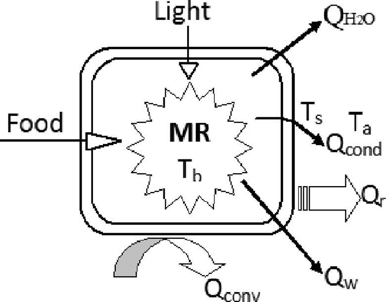
Energy balance in an organism model. Food and light are the 2 major energy sources. Metabolic energy eventually disippates into the environment via body surface radiation (Q _r), convection loss (Q _conv), conduction loss (Q _cond), heat loss through exhalation or evaporation (mainly as latent heat in water vapor, $Q_{H_{2} O}$ ), and heat loss through waste discharge (eg, feces and urine, Q _w).

where Q _r is body surface radiation, Q _conv is convection loss, Q _cond is conduction loss, $Q_{H_{2} O}$ is heat loss through exhalation or evaporation (mainly as latent heat in water vapor and can increase substantially for vigorous activities such as hunting and escaping), Q _w is heat loss through waste discharge, and Q _other is other unknown losses.

The calculation of each component at the right of Equation 2 requires additional efforts in heat transfer. Detailed analysis of each heat component indicated that radiation loss Q _r is the dominant source. As inspired by Kleiber view that metabolism is the fire of life,³³ we can regard all forms of heat losses in Equation 2 are released from an internal, equivalent radiating source (eg, a fire) at a particular body core temperature T _b. So, this will simplify the problem by applying the Stefan-Boltzmann law, which reduces the right of Equation 2 into the following equation:

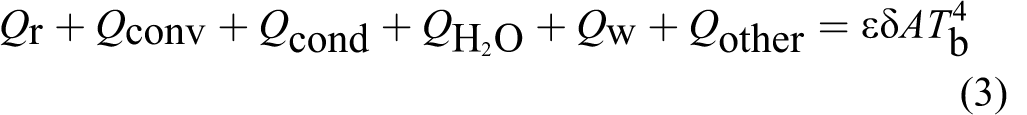
Q_{r} + Q_{c o n v} + Q_{c o n d} + Q_{H_{2} O} + Q_{w} + Q_{o t h e r} = ϵ δ A T_{b}^{4}

From Equations 2 and 3, we get

B M R = ϵ δ A T_{b}^{4}

where ∊ is body emissivity, δ is the Stefan-Boltzmann constant, A is body surface area, and T _b is body core temperature.

Derivation of the Second Scaling Relationship

It is easy to understand that body surface area is related to body mass by the following relationship:

A = {(M / ρ)}^{2 / 3}

Assuming ∊ in Equation 4 and density ρ in Equation 5 are constants, the substitution of Equation 5 into Equation 4 gave Equation 6:

B M R = a M^{2 / 3} T_{b}^{4}

where constant a combines ρ, ∊, and δ. The plot of log MR/T _b ⁴ against log M predicts a straight regression line with a slope of 2/3 and an intercept of log a. However, the presumed “constant” a in Equation 6 actually varies slightly among species due to small differences in body density and body surface characteristics (eg, variations of ρ and ∊ values), resulting in different intercepts of log a for each subgroup as indicated by the short regression lines in Figure 2. The variation in subgroup intercepts will eventually affect the overall mass scaling exponent when the overall regression is conducted for all subgroups (Figure 2A). In addition, the diversity and clustering of subgroups also affect the overall scaling exponent (Figure 2B).

Figure 2.

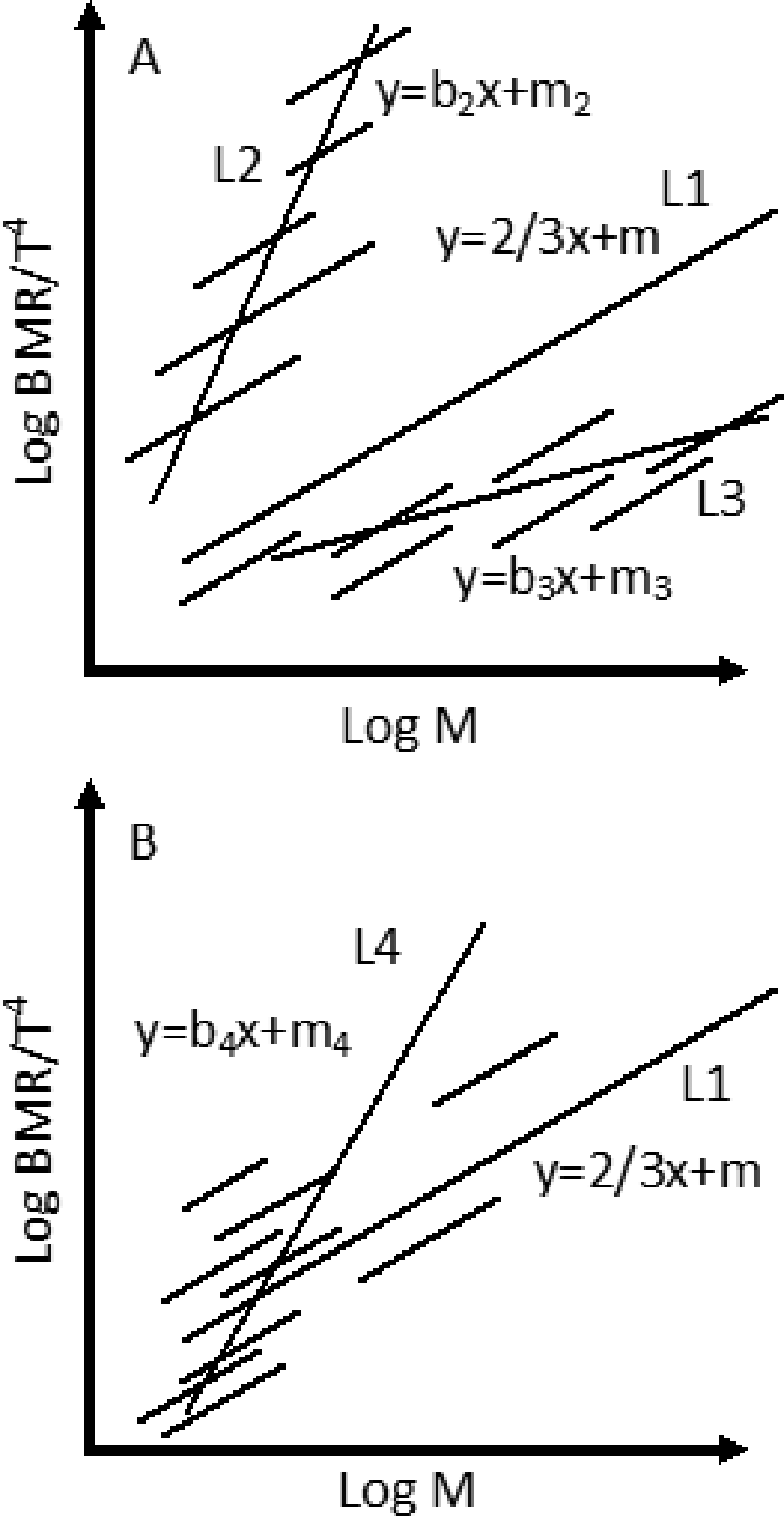
The effects of subgroup variations on the overall regression slope. L1 is a regression line with an expected slope of 2/3. L2, L3, and L4 are the actual regression lines affected by subgroup intercepts and clustering (short line represents a subgroup).

Therefore, a universal mass scaling exponent of 2/3 or 3/4 was found to be impossible. This conclusion echoes recent opinion made by other scholars.³⁴ Instead, the second scaling relationship is given between BMR, body mass, and body core temperature:

B M R = a M^{b} T_{b}^{4}

where b is the mass scaling exponent. Plots of log BMR/T _b ⁴ against log M predict a straight line with slope of b and intercept of log a.

Derivation of the Third Scaling Relationship

Another important biological trait is biological time (t), which can be derived from metabolic rate as well. At basal metabolic conditions, the product of t and BMR is the total amount of metabolic energy (if BMR is in W), or the total volume (V) of oxygen consumed (if MR in mL O₂/h) within the biological time:

V = B M R \times t

Volume is governed by the gas law, so biological time can be obtained from:

t = \frac{V}{B M R} = \frac{n R T_{b}}{P \times B M R}

where P is the gas pressure, R is the gas law constant, and n is the total moles of consumed oxygen within the biological time and assumed to relate to body mass by $n = f M^{d}$ (f and d are constants), so

t = \frac{f M^{d} {R T}_{b}}{P \times B M R}

As the variation of P is negligible, the following equation gave the third scaling relationship between BMR, mass, temperature, and biological time:

B M R = c M^{d} T_{b} t^{- 1}

where c combines all other constants of f, R, and P. A plot of log tBMR/T _b with log M predicts a straight line with slope of d and intercept of log c.

Sources of Validation Data

In order to test the 2 new allometric scaling relationships derived from thermodynamic principles as aforementioned, a large data set with 3622 values for BMR, M, and T _b collated previously by White et al³⁵ was used to test the second scaling relationship for multiple species. This data set includes 469 mammals, 83 birds, 483 reptiles, 1107 fishes, 682 amphibians, 288 insecta species, 102 arachnida species, 59 mammalian hibernators, 30 mammalian daily heterotherms, 133 protists, and 186 prokaryotes. A second data set comprised of 95 mammals with values for BMR, M, T _b, and t was used to test the third scaling relationship. This data set was extracted from an online database, which was previously reviewed, evaluated, and published.³⁶ In addition, the scaling relationships were also validated with several published data sets in toxicological³⁷ and pharmacological studies.^38
–40 All statistical analysis were conducted using the program OriginPro 8.1.⁴¹

Results

The Second Scaling Relationship

Plots of linear regression between log MR/T _b ⁴ and log M for 469 mammals, 83 birds, 483 reptiles, and 1107 fish are presented in Figure 3. Additional results obtained for amphibians, insecta species, arachnida species, mammalian hibernators, mammalian daily heterotherms, protists, and prokaryotes are presented in Table A1. Apparently, the regressions were statistically significant in all subgroups, showing robustness of the second scaling relationship.

Figure 3.

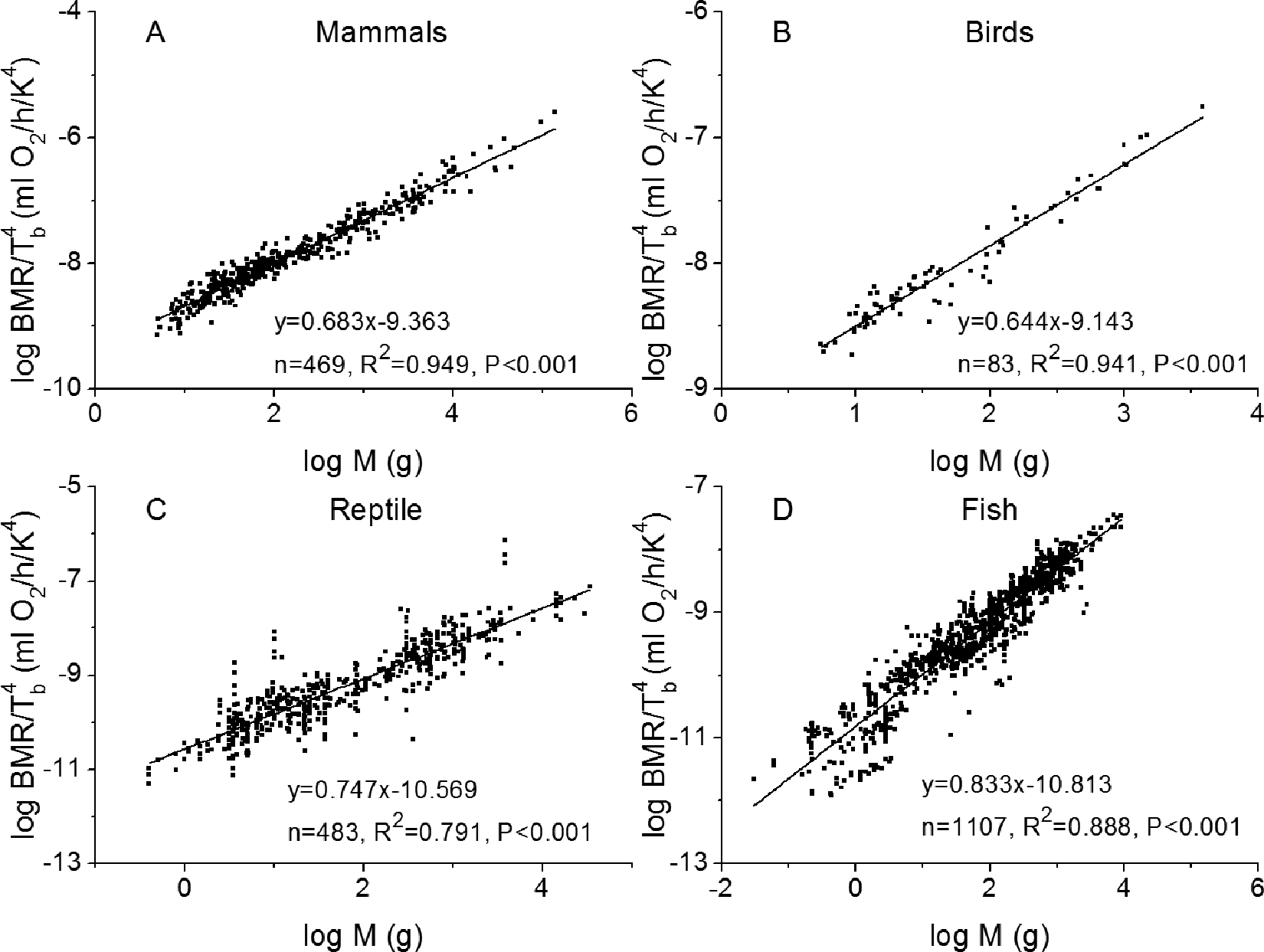
Plots of linear regression between basal metabolic rate, body mass, and temperature for (A) mammals, (B) birds, (C) reptiles, and (D) fish as described by the second scaling relationship in Equation 7. Original units of basal metabolic rate (BMR) in the source data³⁵ were used without conversion.

The Third Scaling Relationship

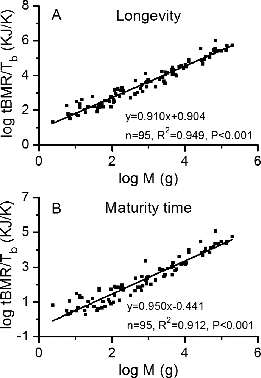
Plots of linear regressions between log tMR/T _b and log M are given in Figure 4 for 95 mammals with values of longevity and maturity time. The correlations were also found to be statistically significant with R ² > 0.912 and P < 0.001. The slopes for longevity and maturity time are close to 1, indicating the assumption of $n = f M^{d}$ made in Equation 10 is actually close to a linear relationship.

Figure 4.

Plots of linear regressions between metabolic rate, body temperature, biological time, and body mass for 95 mammals with (A) longevity and (B) maturity time from published data.³⁶

Discussion

The Second Scaling Relationship and Its Application

As the plots shown in Figure 3, the linear regressions were proved to be statistically significant, indicating robustness of the newly derived scaling relationship. Return to scaling relationship described by Equation 7, the regression results tested with empirical data showed slope differences between mammals, birds, reptiles, and fish (see Figure 3), such differences also existed in other subgroups (see results in Table A1). In addition, the second scaling relationship was tested with 30 unicells and 34 plants,²³ and slope differences were also found in these species (0.722 in Figure 5A and 0.795 in Figure 5B).

Figure 5.

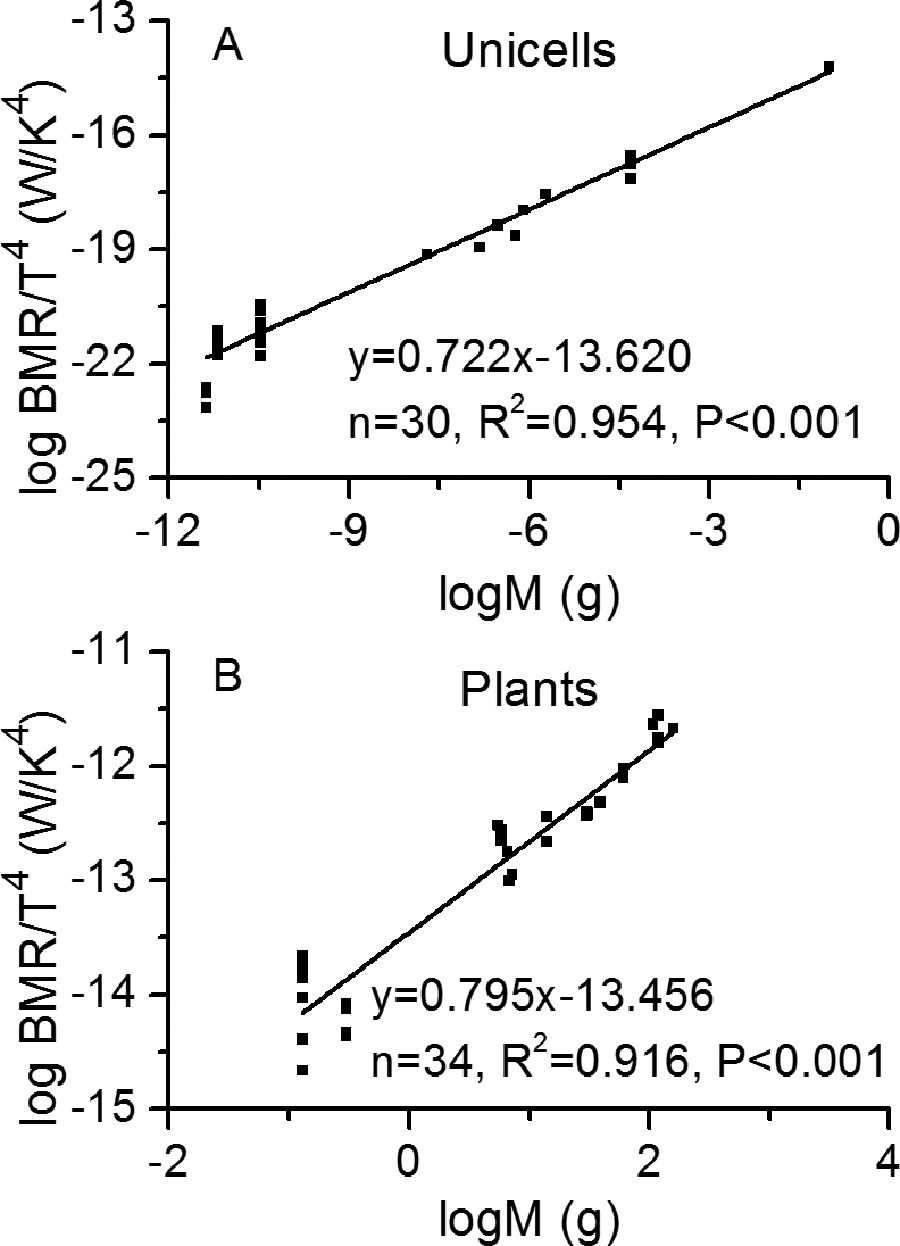
Plots of linear regression between basal metabolic rate, body mass, and temperature for (A) unicells and (B) plants, as described by the second scaling relationship in Equation 7. Original units of basal metabolic rate (BMR) in the source data²³ were used without conversion.

Thus, due to subgroup variations, universal scaling exponent (or the slope) is impossible. Mathematically, the scaling exponent b in Equation 7 varies between zero and infinity as implicated by possible regression lines of L2, L3, and L4 in Figure 2. However, the actual scaling exponent often falls within a range of 0.5 to 1.5 (see Table A1). This is consistent with a wide range of reported exponent values.^42,43

The second scaling relationship and its slope differences among subgroup species have significant implications for toxicity and dose extrapolations. For example, we can easily extrapolate the dose from the first to the second species by:

D_{2} = D_{1} \times \frac{a_{2}}{a_{1}} \frac{M_{2}^{b 2}}{M_{1}^{b 1}} {(\frac{T_{2}}{T_{1}})}^{4}

where D is dose in mg/d, lowercase 1 and 2 represent the first and second species, and T is body core temperature. If the studied species are from the same group with a common scaling exponent of b, then the above-mentioned extrapolation can be reduced to

D_{2} = D_{1} \times {(\frac{M_{2}}{M_{1}})}^{b}

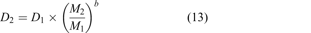
This simple equation has been widely used for the calculation of HED by toxicologists with a scaling exponent of 2/3:

H E D = D_{a} \times {(\frac{M_{h}}{M_{a}})}^{2 / 3}

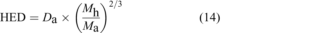
where the units of HED is in mg/d and M in g and lower case h and a for humans and animals. It is worthy of mention to write the following equation for body mass normalized HED_m for humans and D _a,m for animals, which is sometimes mistakenly used due to units problems:

{H E D}_{m} = D_{a, m} \times {(\frac{M_{a}}{M_{h}})}^{1 / 3}

where the units of HED_m is in mg/g/d.

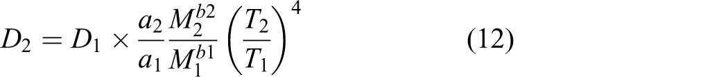
In reality, dose extrapolation is more often conducted for species from different subgroups, thus Equation 12 should be used to account for variations in a, b, and T _b in all subgroups. For example, if we conduct dose extrapolation for a human with body mass of 70 kg and body temperature of 37°C from a reptile with a body mass of 500 g and body temperature of 20°C, the HED value given in Equation 14 were about 15 times lower than results of Equation 12 (a and b values were taken from Table A1 for mammals and reptiles). This means the application of Equation 14 underestimates the desired effects of dose or it overestimates the undesired toxicity. On the contrary, the opposite extrapolation from mammals to reptiles using Equation 14 could sometimes underestimate the risk, causing drug overdosage.

The second scaling relationship was also validated using measured acute toxicity data (maximum tolerated dose [MTD]) compiled by Watanabe et al³⁷ for 23 chemicals from monkeys and dogs to humans. The values of a and b were taken from Table A1 for mammals. Thus, Equation 12 was transformed to Equation 16:

{M T D}_{h} = {M T D}_{a} {(\frac{M_{a}}{M_{h}})}^{0.317} {(\frac{T_{h}}{T_{a}})}^{4}

Using the above-mentioned equation and typical body temperature values,¹¹ good agreement was found between the extrapolated and measured human MTDs either from dog (Figure 6A) or monkey (Figure 6B) toxicity values. This implicates that human toxicity values can be predicted from animal studies with relatively high accuracy based on the second scaling relationship.

Figure 6.

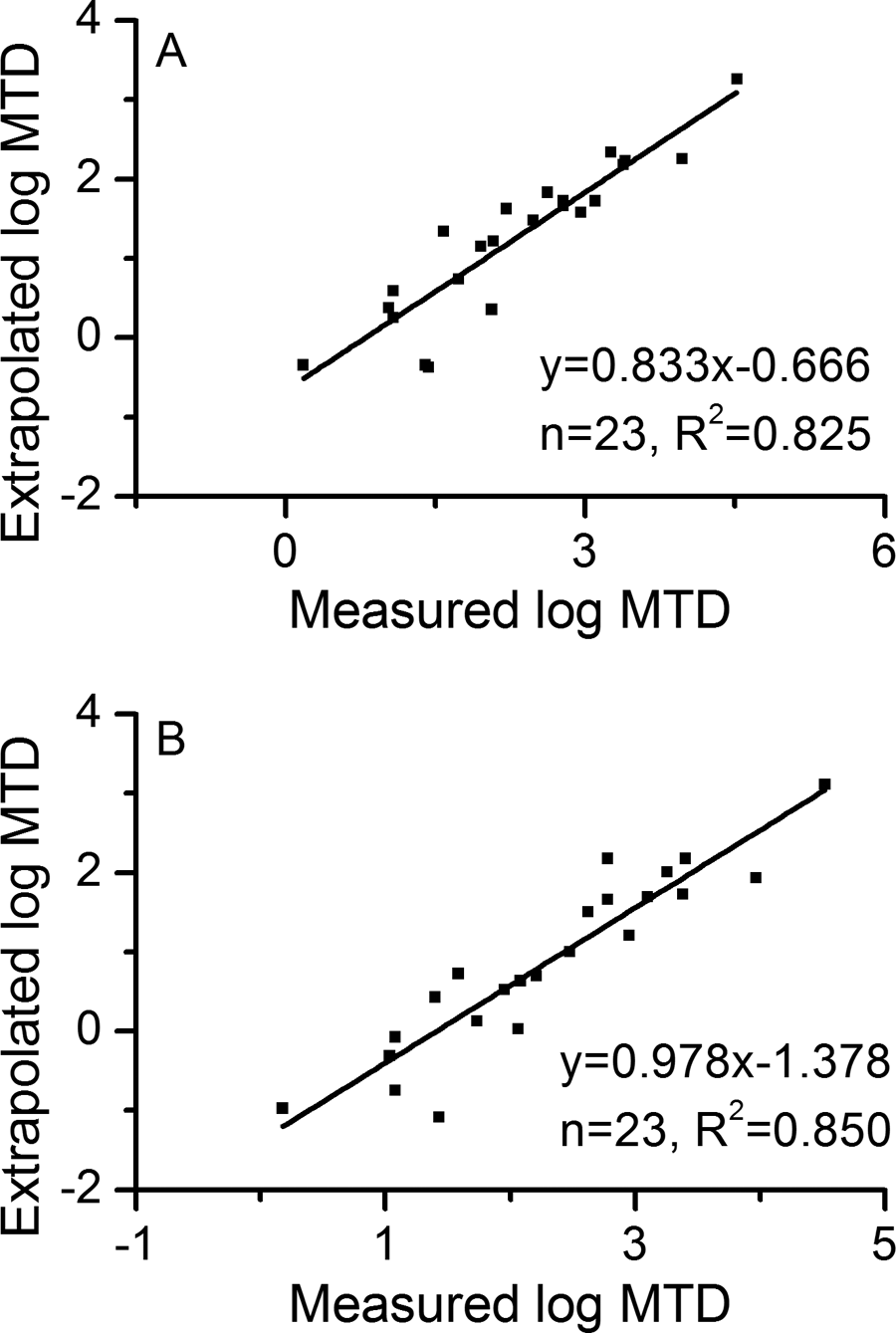
Comparison of extrapolated toxicity values (maximum tolerated dose [MTD]) by the second scaling relationship with measured values in published studies³⁷ for humans: (A) extrapolation from dog and (B) extrapolation from monkey.

The Third Scaling Relationship and Its Application

With the third scaling relationship described by Equation 11, it correlates with all 4 important biological traits of metabolic rate, mass, temperature, and biological time, from which biological time can be expressed as:

t = c M^{d} {(\frac{B M R}{T_{b}})}^{- 1}

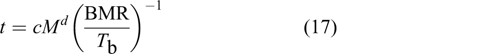
Apparently, biological time is the product of a mass scaling component with the reciprocal of a temperature normalized metabolic rate. In cases of longevity and maturity times, the exponent of d in Equation 17 is close to one as indicated by the slopes in Figure 4. This was also confirmed with the pharmacokinetic half-lives of some drug metabolism studies. For example, half-life values of a novel quinolone, garenoxacin,³⁸ and a sulfamide-containing NK₂ antagonist, UK-224,671³⁹ scales well between rat, monkey, dog, and humans as shown in Figure 7A to C. Although good scalings were also observed for mean residence time (MRT in Figure 7C) and time for maximal plasma concentration (t _max in Figure 7D), the scaling exponents not only deviated significantly from each other (eg, 0.825 for MRT against 0.638 for t _max) but also were much lower than one as observed for pharmacokinetic half-lives, implicating these parameters are probably more drug specific. The discussed examples demonstrated that the third scaling relationship found tremendous potential for the prediction of human pharmacokinetic times (eg, t _1/2, MRT, and t _max) based on animal studies, which are extremely useful in pharmacological studies.

Figure 7.

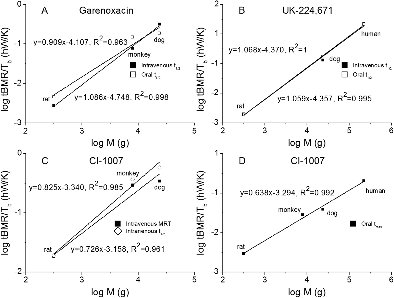
Validation of the third scaling relationship with published pharmacological studies for 3 drugs administered by rat, monkey, dog, and humans via intravenous and oral routes: (A) half-life (t _1/2) for garenoxacin,³⁸ (B) t₁ _/2 for UK-224,671,³⁹ (C) t _1/2 and mean residence time (MRT) for CI-1007 via intravenous administration,⁴⁰ and (D) time for maximal plasma concentration (t _max) for CI-1007 via oral administration.⁴⁰

Conclusions

Based on thermodynamic principles, 2 new allometric scaling relationships were derived between 4 important biological traits, namely BMR, body mass, body core temperature, and biological time. The robustness of new relationships was validated with empirical data, which all proved to be statistically significant. The results also demonstrated that it is impossible to find a universal scaling exponent in reality due to subgroup variations in body characteristics. This implicates that current method of toxicity and dose extrapolation based on existing allometric scaling with single mass exponent of 2/3 or 3/4 could over or underestimate the risk. Therefore, individual extrapolation models should be built to obtain different scaling exponents specific to the interested group of species. These individual models would be practically useful for scaling and extrapolation in ecology, toxicology, pharmacology, and many other areas.^1,7,44

Footnotes

Appendix A

Table A1.

Summary of Linear Regression Results for the Second Scaling Relationship.^a

Subgroup	Coefficients		Statistics
Subgroup	log a	b	n	R ²	P	F
Mammals	−9.363	0.683	469	0.949	<0.001	8648.681
Birds	−9.143	0.644	83	0.941	<0.001	1305.075
Reptile	−10.569	0.747	483	0.791	<0.001	1821.537
Fish	−10.813	0.833	1107	0.888	<0.001	8783.784
Amphibians	−11.008	0.881	682	0.799	<0.001	2700.132
Insecta	−10.358	0.83	288	0.82	<0.001	1301.101
Arachnida	−10.945	0.801	102	0.785	<0.001	365.826
Mammalian hibernator	−10.883	0.877	59	0.857	<0.001	340.482
Mammalian daily heterotherms	−9.975	0.778	30	0.837	<0.001	143.746
Protist	−11.695	0.69	133	0.821	<0.001	600.074
Prokaryote	−7.325	1.266	186	0.554	<0.001	228.656

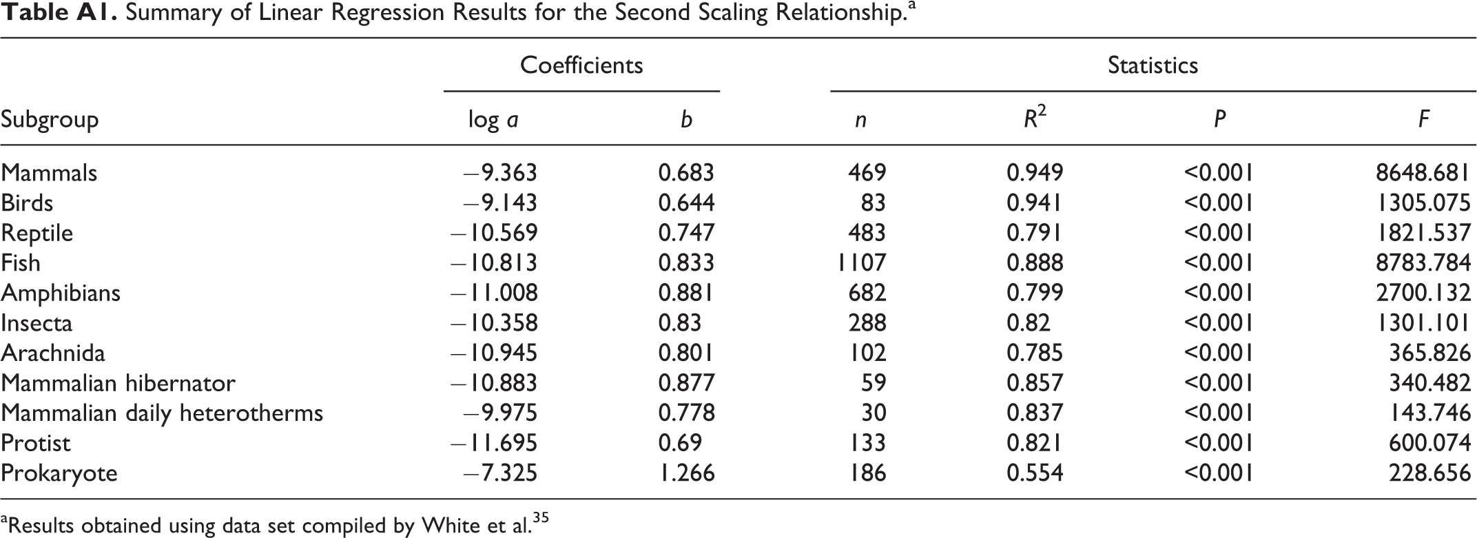
^aResults obtained using data set compiled by White et al.³⁵

Author Contributions

Qiming Cao contributed to acquisition, analysis, and interpretation; drafted the manuscript; critically revised the manuscript; gave final approval; and agrees to be accountable for all aspects of work ensuring itegrity and accuracy. Jimmy Yu contributed to analysis and interpretation, drafted the manuscript, critically revised the manuscript, gave final approval, and agrees to be accountable for all aspects of work ensuring itegrity and accuracy. Des Connell contributed to interpretation, drafted the manuscript, critically revised the manuscript, gave final approval, and agrees to be accountable for all aspects of work ensuring itegrity and accuracy.

Declaration of Conflicting Interests

The author(s) declared no potential conflicts of interest with respect to the research, authorship, and/or publication of this article.

Funding

The author(s) declared the following financial support for the research, authorship, and/or publication of this article: This work was supported by a UESTC Scientific Research Fund from the Ministry of Education of the People’s Republic of China. The author also benefited from earlier work supported by the ARC-Spirt Program from Australia Research Council.

References

West

Brown

. The origin of allometric scaling laws in biology from genomes to ecosystems: towards a quantitative unifying theory of biological structure and organization. J Exp Biol. 2005;208 (pt 9):1575–1592.

Schmidt-Nielsen

. Scaling: Why is Animal Size So Important? Cambridge, United Kingdom: Cambridge University Press; 1984.

McMahon

Bonner

. On Size and Life. New York: W.H. Freeman and Company; 1983.

Kleiber

. Body size and metabolism. Hilgardia. 1932;6 (11):315–353.

Biewener

. Biomechanical consequences of scaling. J Exp Biol. 2005;208 (9):1665–1676.

White

Seymour

. Allometric scaling of mammalian metabolism. J Exp Biol. 2005;208 (9):1611–1619.

Marquet

Quinones

Abades

. Scaling and power-laws in ecological systems. J Exp Biol. 2005;208 (9):1749–1769.

Hoppeler

Weibel

. Scaling functions to body size: theories and facts. J Exp Biol. 2005;208 (9):1573–1574.

Savage

Gillooly

Woodruff

. The predominance of quarter-power scaling in biology. Funct Ecol. 2004;18 (2):257–282.

10.

Daugherty

. Assessment of Chemical Exposures: Calculation Methods for Environmental Professionals. Boca Raton: CRC Press; 1997.

11.

Derelanko

. The Toxicologist's Pocket Handbook. Boca Raton: CRC Press; 2008.

12.

Derelanko

Auletta

, eds. Handbook of Toxicology. Boca Raton: CRC Press; 2008.

13.

Food and Drug Administration. Guidance for Industry Estimating the Maximum Safe Starting Dose in Initial Clinical Trials for Therapeutics in Adult Healthy Volunteers. Washington, DC: Food and Drug Administration, US Department of Health and Human Services; 2005:30.

14.

US Environmental Protection Agency. Recommended Use of Body Weight 3/4 as the Default Method in Derivation of the Oral Reference Dose. Washington, DC: US Environmental Protection Agency; 2011.

15.

Vermeire

Stevenson

Pieters

Rennen

Slob

Hakkert

. Assessment factors for human health risk assessment: a discussion paper. Crit Rev Toxicol. 1999;29 (5):439–490.

16.

Sarrus

Rameaux

. Application des sciences accessoires et principalement des mathématiques à la physiologie générale. Bull Acad R Méd. 1839;3:1094–1100.

17.

Rubner

. Concerning the influence of body size on energy metabolism. Z Biol. 1883;19:536–562.

18.

Heusner

AA.

Energy metabolism and body size. I. Is the 0.75 mass exponent of Kleiber's equation a statistical artifact?

Respir Physiol. 1982;48 (1):1–12.

19.

Feldman

McMahon

. The 3/4 mass exponent for energy metabolism is not a statistical artifact. Resp Physiol. 1983;52 (2):149–163.

20.

Schuster

. Power laws in biology. Complexity. 2010;16 (3):6–9.

21.

McMahon

. Size and shape in biology. Science. 1973;179 (4079):1201–1204.

22.

West

Brown

Enquist

. A general model for the origin of allometric scaling laws in biology. Science. 1997;276 (5309):122–126.

23.

Gillooly

Brown

West

Savage

Charnov

. Effects of size and temperature on metabolic rate. Science. 2001;293 (5538):2248–2251.

24.

de Castro

Gaedke

. The metabolism of lake plankton does not support the metabolic theory of ecology. Oikos. 2008;117 (8):1218–1226.

25.

Duncan

Forsyth

Hone

. Testing the metabolic theory of ecology: Allometric scaling exponents in mammals. Ecology. 2007;88 (2):324–333.

26.

Price

Weitz

Savage

. Testing the metabolic theory of ecology. Ecol Lett. 2012;15 (12):1465–1474.

27.

Terblanche

Janion

Chown

. Variation in scorpion metabolic rate and rate-temperature relationships: implications for the fundamental equation of the metabolic theory of ecology. J Evolution Biol. 2007;20 (4):1602–1612.

28.

Savage

Deeds

Fontana

. Sizing up allometric scaling theory. PLoS Computat Biol. 2008;4 (9):1–17.

29.

Kolokotrones

Savage

Deeds

Fontana

. Curvature in metabolic scaling. Nature. 2010;464 (7289):753–756.

30.

Dodds

Rothman

Weitz

. Re-examination of the “3/4-law” of metabolism. J Theor Biol. 2001;209 (1):9–27.

31.

Clarke

. Temperature and the metabolic theory of ecology. Funct Ecol. 2006;20 (2):405–412.

32.

Stumpf

MPH

Porter

. Critical truths about power laws. Science. 2012;335 (6069):665–666.

33.

Kleiber

. The Fire of Life: An Introduction to Animal Energetics. New York: Wiley; 1961.

34.

White

. PHYSIOLOGY There is no single P . Nature. 2010;464 (7289):691–693.

35.

White

Frappell

Chown

. An information-theoretic approach to evaluating the size and temperature dependence of metabolic rate. Proc R Soc B Biol Sci. 2012;279 (1742):3616–3621.

36.

Tacutu

Craig

Budovsky

. Human Ageing Genomic Resources: Integrated databases and tools for the biology and genetics of ageing. Nucleic Acids Res. 2013;41 (database issue):D1027–D1033.

37.

Watanabe

Bois

Zeise

. Interspecies extrapolation: a reexamination of acute toxicity data. Risk Anal. 1992;12 (2):301–310.

38.

Hayakawa

Fukushima

Kato

. Metabolism and disposition of novel des-fluoro quinolone garenoxacin in experimental animals and an interspecies scaling of pharmacokinetic parameters. Drug Metab Dispos. 2003;31 (11):1409–1418.

39.

Beaumont

Harper

Smith

Abel

. Pharmacokinetics and metabolism of a sulphamide NK2 antagonist in rat, dog and human. Xenobiotica. 2000;30 (6):627–642.

40.

Feng

Loo

Wright

. Disposition of the antipsychotic agent Cl-1007 in rats, monkeys, dogs, and human cytochrome P450 2D6 extensive metabolizers—species comparison and allometric scaling. Drug Metab Dispos. 1998;26 (10):982–988.

41.

OriginPro . Version 8.1. Northampton, MA: OriginLab Corporation; 2010.

42.

da Silva

JKL

Barbosa

Silva

. Unified theory of interspecific allometric scaling. J Phys A Math Theor. 2007;40 (44):F953–F959.

43.

White

Seymour

. Does basal metabolic rate contain a useful signal? Mammalian BMR allometry and correlations with a selection of physiological, ecological, and life-history variables. Physiol Biochem Zool. 2004;77 (6):929–941.

44.

Sharma

McNeill

. To scale or not to scale: the principles of dose extrapolation. Br J Pharmacol. 2009;157 (6):907–921.

New Allometric Scaling Relationships and Applications for Dose and Toxicity Extrapolation

Abstract

Keywords

Introduction

Methods

Thermodynamic Basis

Derivation of the Second Scaling Relationship

Derivation of the Third Scaling Relationship

Sources of Validation Data

Results

The Second Scaling Relationship

The Third Scaling Relationship

Discussion

The Second Scaling Relationship and Its Application

The Third Scaling Relationship and Its Application

Conclusions

Footnotes

Appendix A

Author Contributions

Declaration of Conflicting Interests

Funding

References