Hypothesis Testing in High-Throughput Screening for Drug Discovery

Abstract

Following the success of small-molecule high-throughput screening (HTS) in drug discovery, other large-scale screening techniques are currently revolutionizing the biological sciences. Powerful new statistical tools have been developed to analyze the vast amounts of data in DNA chip studies, but have not yet found their way into compound screening. In HTS, characterization of single-point hit lists is often done only in retrospect after the results of confirmation experiments are available. However, for prioritization, for optimal use of resources, for quality control, and for comparison of screens it would be extremely valuable to predict the rates of false positives and false negatives directly from the primary screening results. Making full use of the available information about compounds and controls contained in HTS results and replicated pilot runs, the Z score and from it the p value can be estimated for each measurement. Based on this consideration, we have applied the concept of p-value distribution analysis (PVDA), which was originally developed for gene expression studies, to HTS data. PVDA allowed prediction of all relevant error rates as well as the rate of true inactives, and excellent agreement with confirmation experiments was found.

Introduction

High-throughput screening (HTS) is considered to be the famous search for the needle in the haystack. This often referred-to picture describes the fact that in the majority of drug discovery screens, only a small number of active substances is searched for within a large number of inactive substances. This imbalance is the whole reason for performing random screening experiments, where “substance” can refer to anything from small organic molecules, natural products, peptides, RNA, to proteins or even cells. The purpose of primary screening, the first assay en route to an optimized medicine, is to arrive at a short list of mostly active compounds, starting from the large list of mostly inactive compounds, at a manageable consumption of material and resources. The primary hit list can only serve as a candidate set of possibly active compounds, because it is generated free of any prior hypothesis as to which of the compounds are expected to be active and which ones are expected to be inactive. Therefore, confirmation experiments have to follow to establish the real activity of the hit list members. From the details of the workflow, i.e., primary screen – hit list generation – confirmation of the hits, it is obvious that primary false negatives will never be followed later on. Only if additional knowledge in the form of structure-activity relationships is taken into account can weakly active compounds be rescued, that have interesting physico-chemical or pharmacokinetic properties. Vice versa, a lot of primary false positives unnecessarily increase the cost of follow-up experiments. The ideal hit list is a balance between these two counteracting consequences.

In order to arrive at this balance, a detailed characterization of the primary hit list is required. To stay in the illustrative picture: how many needles are in the haystack? For a certain hit list cutoff, how many needles will be found, how many will be missed, and how many are actually straws? Or, more seriously: how many more confirmed hits can be found if 1000 compounds more are retested? How many compounds have to be retested to achieve a false negative rate of less than 50%? And, most fundamental, are the hits in the list significant at all?

In the current situation, intuitive ad hoc visual inspection by an experienced senior screening expert is a common way to characterize the hit list distribution; hit selection is often determined by the retesting capacity rather than by statistical considerations; often no quantitative information of the quality of the primary hit list is available before confirmation experiments are finished; statistical methods are largely neglected, partly due to the fact that no replicates are available for full-library screens.

The characterization of primary screens has improved over the past years, most notably with the long-awaited introduction of a unified quality criterion, the Z′ factor, ¹ and after robust estimates for the mean and the standard deviation got in use, for instance, with the so-called B-score.^2,3 Nevertheless, there is still a need for quantification tools of hit list properties, i.e., estimates of the false positive rate (FPR), the false negative rate (FNR), the false discovery rate (FDR, 1-confirmation rate), for quality control and prioritization of confirmation experiments.

It is important to emphasize that the present work only makes statements about sensitivity and specificity from statistical variation. Reproducible assay artifacts that lead to erroneous hits or underestimated activities for individual compounds are not taken into account and cannot be investigated with the method presented here.

In contrast to pharmaceutical HTS, statistical analysis of high-throughput data has been developed and applied since the early days of DNA microarrays for gene expression profiling. A vast body of tools is available ^4,5 and standardized data quality control is nowadays a widely accepted procedure ^6,7 and required by many high-ranking journals upon publication. One difference is that, unlike in HTS with only one data point per compound, at least three DNA chips are usually analyzed per group to estimate the biological variability of each gene. With only one measurement per compound in HTS, it is impossible to estimate the variance of each individual compound. Hence, it is a common conviction that the tools and concepts used in and developed for genomic analyses cannot be utilized for chemical library HTS data. It will be demonstrated below that by exploiting the information from replicated positive and negative controls on each microwell plate, and by disseminating replicated pilot screens, assay variability can be estimated with sufficient accuracy also in pharmacological HTS.

As a first step in the hit list characterization procedure proposed here, the hit selection process is considered as a statistical test. In particular, Fisher’s Z-test is applied to find compounds significantly more active than inactive controls or than a preset minimum activity. The assumptions required for the Z-test are evaluated on the basis of a medium scale pilot screen including some 10 000 compounds and controls that span the whole range of activities from 0 to 100 percent. For the actual test, the mean and standard deviation under the Null hypothesis H₀, i.e., the inactive population, are calculated robustly (median and median absolute deviation) from negative controls or from the entire compound data, assuming a small rate of active compounds. For characterization of the hit list including, for instance, FDR and FNR, the p-value distribution analysis method proposed by John D. Storey for microarray data ^8,9 is introduced because of its intuitive usage and because it can be extended to multiple dimensions in a straightforward way. Finally, the predicted FDR is compared to confirmation experiments for five actual screens of different kinds and found to be highly accurate.

P-value distribution analysis (PVDA) holds promise to provide a solid quantitative understanding of the quality of primary HTS hit lists, to rationalize the extent of confirmation experiments and to facilitate data-driven prioritization of resources.

Materials and Methods

Large-Scale Screening as a Multitude of Statistical Tests

Rigorous statistical analysis of HTS data was rather limited in the past, at least partly because for most of the often one million compounds no replicates are available. In contrast, in gene expression profiling using DNA microarrays, statisticians were involved in data analysis at a time when the field was still in its infancy. As a consequence, a large and ever-growing body of statistical data analysis tools has been and is being developed.

In a typical microarray (chip) experiment, two or more groups of subjects, either true individuals or pooled individuals, are compared. For the sake of simplicity, let us assume two groups of individuals are different according to one treatment of interest and any stratifying variable shall be neglected for the moment. Replicated measurements are taken to estimate the distribution of expression for each gene because it can vary considerably from one gene to the other. The number of possible replicates is usually rather small due to the relatively high costs of the experiment. Fortunately, in many practical cases it is allowed to assume a normal distribution of the expression level fold changes and to apply the t-test. ¹⁰ As a consequence, acceptable statistical power is often achieved already with three to five good quality replicates by applying the shrinkage approach, where the variance estimate of each particular gene is stabilized by taking the variance of all other genes into account. ¹¹

Between the two groups, one statistical test is performed for each RNA transcript represented on the chip, about 50 000 for a human whole-genome chip. With such a large number of tests, the so-called “multiple testing problem” is easily illustrated in the following.

Consider a p-value cutoff for each individual test, p₀ ( Fig. 1a ). Then, the probability of finding at least one false positive test among the N genes when in fact both groups are identical, can be approximated as ptot ≤ Np₀ (Bonferroni). As discussed by Benjamini and Hochberg, ¹² in the multiple testing situation the relevant criterion to determine a hit list cutoff is rather, how many false positive results are expected for each positive finding (false discovery rate). For instance, in a full library screen of one million compounds, if the maximally accepted p value for each test is set to be as high as 5%, we would expect to observe 50,000 positives even when all compounds are really inactive. For cases where the number of tests is as large as in whole genome or full library experiments (N > 1000), John D. Storey has introduced an illustrative way to estimate the false discovery rate ⁸ and thus determine a statistically derived hit list cutoff. His line of argument will be followed for the remaining part of this work.

Figure 1.

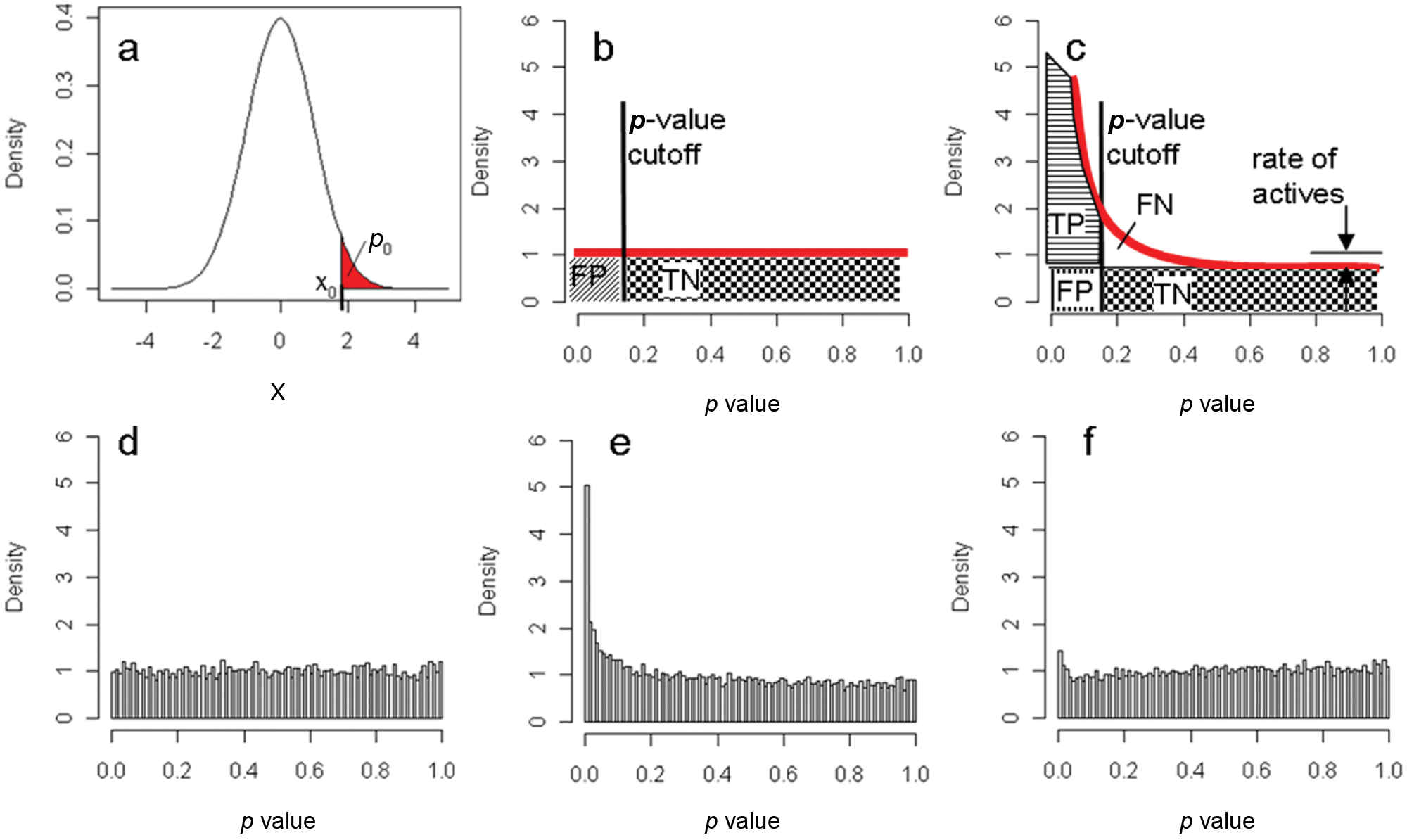
(a) Definition of the p value. For any value x₀ of a test statistics x, the p value p₀ is the probability of observing this value x₀ or an even more extreme value (red area). (b) Schematic of the uniform PVD under H₀ (red line), (c) of a mixture of observations from H₀ and different alternative hypotheses. (d) and (e) show PVDs based on simulated data, corresponding to the conditions (b) and (c), respectively. The irregular PVD (f) is obtained from the same data as in (e) but with an overestimation of the standard deviation by 10%, resulting in the dip at around p = 0.06.

The p-Value Distribution Analysis

The false discovery rate can be estimated by analyzing the distribution of p values that were calculated from any meaningful statistical test in a correct manner, i.e., by assuring that the derived p value really corresponds to the true type-1 error rate. In this case, the p-value distribution (PVD) for observations obeying the Null hypothesis H₀ is uniform by definition. This is due to the fact that the probability From this it follows that, independent of p, i.e., constant. From the schematic PVD of an H₀ ensemble in Figure 1b it becomes clear that a hit list generated by ranking or by a fixed p-value cutoff can contain many hits but they might all be false positives.

In most screening applications, in which the observations are coming from a mixture of many observations obeying the Null hypothesis and only a few obeying the alternative hypothesis, the shape of the PVD is similar to the one shown in Figure 1c , e : a peak at small p values which decreases monotonically toward the horizontal part at large p values. The two cases in Figure 1b , d and 1c , e are representing the only possible regular PVDs for a two-sided test. Any other behavior, such as a dip at low p values or a bump somewhere, is an indication for an irregular behavior of the data or incorrectly determined p values ( Fig. 1f ). Moreover, if no peak at low p values is visible the candidate list will have a very low confirmation rate.

From the horizontal part of the PVD, the rate of Null observations can be directly read as the plateau value of the PVD ( Fig. 1c ). This is a unique feature of the multiple testing situation and not accessible otherwise. Once a p-value cutoff is given, all relevant error rates can be directly read from the PVD. The hit rate is given by the area to the left of the cutoff; the true positive rate is equal to the area to the left of the cutoff and above the plateau; the false positive is equal to the area to the left of the cutoff and below the plateau. The false negative rate is equal to the area to the right of the cutoff and above the plateau; the true negative rate is equal to the area to the right of the cutoff and below the plateau.

It is now straightforward to determine the p-value cutoff that gives a desired FDR which is equal to the area to the left of the cutoff and above the plateau divided by the total area to the left of the cutoff. The estimated FDR, also called the q value, is conveniently calculated with the help of Storey’s package q value for the statistics software R. ¹³

Multivariate Testing and Hit Selection

The concept of selecting a hit list according to a predefined FDR cutoff using the PVD is readily generalized to the multivariate case. In certain situations the interesting observations may be selected not only according to one criterion but according to a combination of several selection criteria. In pharmaceutical screening this is often referred to as high-content screening (HCS), which describes in the most general meaning of the word a scoring based on more information than just one parameter. In the more common meaning, HCS describes the scoring based on multiple variables (analogous for parameters or readouts) that are determined from two or three dimensional image recordings from cells or tissue sections via image segmentation, object classification, and feature extraction. The features include geometrical properties of the objects, such as area (in number of pixels), circumference, long axis length, or ellipticity, and intensity properties, i.e., any pixel intensity statistics (mean, median, sum, …) in a certain object region, such as the cell membrane, or the cell nucleus, for a certain population of objects.

The p value for the multivariate case can in principle be estimated from the test statistics for any arbitrary multivariate joint probability distribution from pure H₀ samples, i.e., negative controls, or by resampling methods, such as bootstrap. While this might be feasible for univariate scoring, it is often beyond reach for the multivariate situation because the necessary sample size increases roughly with the power of the number of parameters.

A more realistic scenario can be obtained when the data are at least approximately described by the multivariate normal distribution. Then the relevant test statistics is the so- called Mahalanobis distance, m, which is related to the multivariate t statistics as $m_k=t_k^2={\displaystyle \sum _i{(x_{ki}-{\mu }_i)}^2/{\sigma }_i^2}$ , where µ_i, σ_i are mean and standard deviation of the parameter i, and x _ki is the value of parameter i in observation k. Under H₀, m is chi-square distributed, m ~ χ². Thus, the chi-square test in the multivariate case is analogous to the t-test in the univariate case ¹⁴ and known as test of Hotelling or referred to as multivariate analysis of variance (MANOVA).

Multivariate testing is not widely used in statistics because of the so-called curse of the dimensions: the refutation range of the test statistics, e.g., the typical 5% quantile of the Mahalanobis distance, is decreasing linearly with the number of dimensions. In geometrical terms, the outer 5% slice of the N-dimensional hypervolume is getting thinner and thinner as the number of dimensions increases. As a consequence, the univariate test has more power than the multivariate test; here, power means the statistical term describing the ability to detect a real difference, i.e., the true positive rate. Therefore, in any HCS application, a possible gain in information by integration of an additional parameter has to balance the loss in testing power.

Especially for cases where subsets of parameters are correlated to a different degree with each other but uncorrelated with other subsets several dimension reduction methods are available, ¹⁵ such as principal component analysis (PCA). They are also essential operations prior to hypothesis testing because in general the tests require independence of the individual measurement.

Experimental

For validation of the theoretical predictions for the FDR they are compared to actual screening data coming from a range of experimental situations. The data include biochemical and cellular assays, different target classes, such as, GPCRs or proteases, and different assay readouts, such as, fluorescence resonance energy transfer (FRET) for second messenger quantification or polarization anisotropy for detecting ligand binding.

The ~1 Mio compounds from the Roche screening library are plated in an arbitrary nonrandomized fashion in column 3 through 24 of a 384-well plate. During HTS, columns 1 and 2 are filled with a number of controls of different kind depending on the type of assay. Typically, these consist of three concentrations of a known effective reference compound with defined activities, such as, 0%, 50%, and 100% that are used later for normalization and quality control (QC). Experiments were performed at the Roche Basel screening facility.

QC and visual inspection of the raw data is done using Genedata’s Screener software (Genedata AG, Basel, Switzerland). The positive (-100%) and negative (0%) controls are used for plate-wise normalization of the signal to correct for additive and multiplicative plate-to-plate or daily variability of the sensitivity window of the assay. The normalized signal reads as

$$S_{norm}=\frac{S_{raw}-{\tilde{S}}_{neg}}{{\tilde{S}}_{pos}-{\tilde{S}}_{neg}},{\tilde{S}}_{neg}=\text{MEDIAN}\left(S_{neg}^i\right){\tilde{S}}_{pos}=\text{MEDIAN}\left(S_{pos}^i\right).$$

The software also allows for correction of between-plate patterns from systematic tip carry-over or clogging, or persistent within-plate patterns from temperature edge effects or gradients according to an undisclosed method. Correction is carried out only if necessary and only if it improves the apparent geometric patterns in the signal, as judged by visual inspection.

The FDR prediction is compared to the experimentally determined confirmation rate (1 - FDR) from concentration- response hit confirmation screens. The experimental false negative rate is compared with the prediction within a specific interval bounded on the one hand by the hit confirmation cutoff and on the other hand by the FDR cutoff, as given in the results section.

Hit confirmation experiments were carried out using the same plate and liquid handling robotic systems and the same readers as in the primary screen. Between-plate serial dilutions were prepared to obtain 12-point concentration response curves. A confirmed hit is defined as a compound for which the normalized activity at the screening concentration calculated from the concentration response is further away from the negative control than the cutoff: smaller than the cutoff for inhibitory assays and larger than the cutoff for activation assay. This phrasing takes into account the fact that in our convention the positive controls in antagonist assays correspond to -100 % activity while in agonist assays the positive control is at +100 %.

Results

The p-value distribution analysis method described in the methods section was validated on five screening campaigns as described in the experimental section. First, replicate pilot screens were analyzed to ensure that the assumptions of PVDA are in general sufficiently fulfilled for this type of assay. Next, the same assumptions are probed for the actual primary screening data as far as possible, with replicates available just for control compounds and single values for the test compounds. This step is important because the data variability is often different in the pilot as compared with the primary screen. Finally, the predicted rate of actives in the set of compounds retested in confirmation experiments is compared with the actual outcome.

Distribution of Compounds and Controls

Down to its foundation, PVDA depends on the correctness of the applied test. For the Z-test it means that for each compound, observations need to be independent and identical normally distributed each with the same variance but different means. It is clear from the very beginning that this assumption will not be fulfilled in a strict sense. Rather, the relevant question is going to be, how much will it be violated and what are the consequences. Fortunately, by visually analyzing the PVD we have an internal control allowing characterization of the influence of any gross deviation.

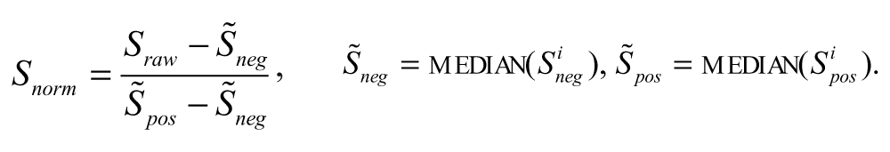
One powerful tool to compare data distributions with each other or with theoretical distributions is the so-called quantile-quantile plot, or QQ-plot (an example is shown in Fig. 2b ). If two distributions are the same, all their properties, including the quantiles, are identical. If the sample quantiles are plotted against the reference quantiles of two identical distributions, the data are located along a straight line. If the sample distributions contain more extreme values as expected, i.e., if it is long-tailed compared to the reference distribution, the QQ-plot exhibits points below the line on the left end of the data range and above the line on the right end ( Fig. 2b ); for short-tailed distributions it is the opposite; for right-skewed distributions, the points are above the line on both ends of the data range; for left-skewed distributions they are below on both ends. In the QQ-plot, the behavior of the tails is more strongly visible than the behavior of the center, just the opposite as compared with a histogram, where often the tail behavior is invisible.

Figure 2.

Characterization of compound and control activities during a pilot screen. (a) Point series of consecutive measurements. (b) Histogram and QQ-plot of the negative controls. (c) Two-run reproducibility plot. (d) Median of the standard deviation of two runs as a function of the median of the 2-run mean.

In order to guarantee that the data are independent identical normal distributed, two criteria shall be checked: (i) the overall frequency distribution is sufficiently close to a normal distribution, as illustrated by the QQ-plot and tested formally using the Kolmogorov-Smirnov test (H₀: data are normal: p = 0.14); (ii) the variance is independent of the mean, as judged visually from a plot median{(x₁-x₂)/√2} against median{(x₁+x₂)/2}, where x₁, x₂ are replicates of the same compound or control in a pilot screen.

This and other general quality control plots are shown in Figure 2 . Visualization is one of the most important methods for descriptive data analysis especially when dealing with large data sets or multiple dimensions. Figure 2a displays the series of data from three replicates of a pilot screen consisting of close to 35,000 data points from ninety-nine 384-well plates. Data were normalized to the medians of the negative and the positive control and corrected for geometric patterns as described. Color coding allows spotting of run-wise signal shifts or drifts of compounds or controls, as well as systematic changes of the variance during the pilot screen. The variance of the negative (red) and the positive control (green) are fairly constant, with a slightly less varying signal around data point 20,000 as compared to 10,000 or 30,000. The intermediate control is constant as expected, with a tiny step at around 23,000. The compounds’ signals cumulate around 0 with sparse outliers toward -100, just as expected.

The distribution of the negative controls and their QQ-plot show no signs for a strong deviation from a normal distribution ( Fig. 2b ). One outlier at around -40 causes the histogram to exhibit a long left tail. This is reflected in the QQ-plot by the point far below the straight line on the left-hand side. The controls from the independent replicates are highly reproducible with little bias ( Fig. 2c ), with a slightly decreasing variability from positive to intermediate to negative control. In 99% of the cases, the difference between the activities in the two runs is less than 15, 14, and 8 for the positive, intermediate, and negative control, respectively. Among the compound signal data points, less than one in a thousand can be considered outliers in at least one run (points along the axis run1 = 0 or run2 = 0) and most are nicely consistent between runs (points along the line run1 = run2). That means, about one in ten hits would be a false positive due to sporadic outliers. The standard deviation of compounds and negative controls is slightly smaller than that of the positive and intermediate controls ( Fig. 2d ). The difference from 3 to 2 over the whole activity range, i.e, 0.1 every 10% activity difference can safely be considered as constant.

To summarize the evaluation of the pilot screen, there are no indications from the data that the necessary assumptions to apply the Z-test are not fulfilled. Apart from a few outliers, the variance estimate from three independent repetitions is independent of the mean.

Parameter Estimation

The primary screen is initiated when the pilot has reached the preset QC criteria for reproducibility and Z′. Because the primary screen is often performed under similar but not identical conditions – a different cell or enzyme batch is used – the variance of the negative control, which is the relevant variable needed for performing the test, cannot be estimated from the pilot.

Essential QC plots for the primary screen are displayed in Figure 3 . Plate-wise 25, 50, and 75% quantiles ( Fig. 3a top) exhibit a larger variability of the inter-quartile range (IQR) than was expected from the pilot screen. The relatively small number of replicates of the controls on each plate results in a rather noisy estimate of the plate-wise variability. This limitation can be overcome by averaging over controls in neighboring plates, i.e., plates that have been measured one after the other, with the idea that they were recorded under similar conditions and therefore their variability should be similar. In the current example, the sliding median absolute deviation (MAD) of controls and compounds is depicted in Figure 3a bottom and serves as the robust estimator of the variance under H₀ for all compounds on a given plate. The smoothing parameter is chosen such that variations across several plates are captured while the large noise in the top panel is suppressed by averaging over approximately 50 wells or five plates. The negative control and the compounds exhibit similar variation, whereas the positive and intermediate controls vary sometimes five times stronger. This can be due to differences in the liquid handling. The median MAD over the whole screen of 2800 plates is similar for all controls and the compounds between 2 and 3.

Figure 3.

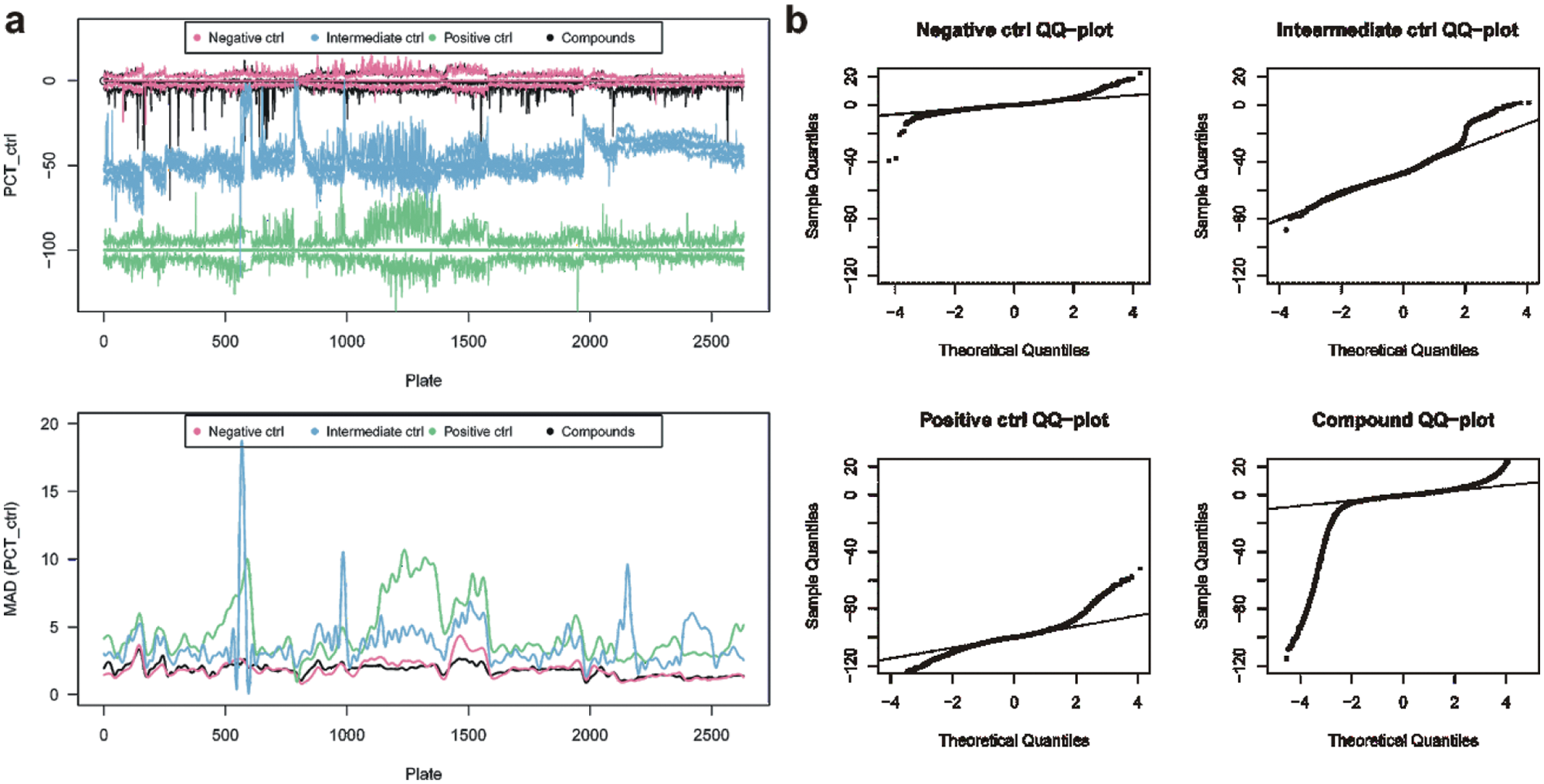
Characterization of compound and control activities during a primary screen. (a) Top: plate medians (center line) plus the 25% and 75% quantiles; bottom: local polynomial smoothing of the plate-wise MAD for controls and compounds. (b) QQ-plot of all controls and of the compounds.

Figure 3b shows QQ-plots for the three controls and the compounds. The negative controls are approximately normal distributed up to 3σ, the intermediate control even up to 4σ, would it not be for the gross outlier region around plate number 520 ( Fig. 3a , top). The positive control distribution is more long-tailed and can only be approximated by a Gaussian inside 2σ. The compounds are clearly skewed toward negative values beyond 3σ.

Predictions from the p-Value Distribution

Using the smoothed robust estimator for the variance of the negative controls on each plate, and their smoothed median as the robust estimator for the plate-wise sample mean under H₀ (activity x = 0), a Z-test is performed for each compound with x < 0, 549,298 in total. The corresponding p value and the normalized activity are illustrated in the one-sided volcano plot, or Geyser plot, in Figure 4b . The spread of the data points is a result of the different assay variability on each plate. If a constant variance is assumed for the whole screen, the graph would exhibit a continuous line. The volcano plot is a popular graphical tool to select hit lists because the significance (p value) of an observation, or more precisely, the negative logarithm, is related to its amplitude (effect size): highly potent substances can be chosen even though their significance is low; similarly, highly significant but weak signals may be rejected.

Figure 4.

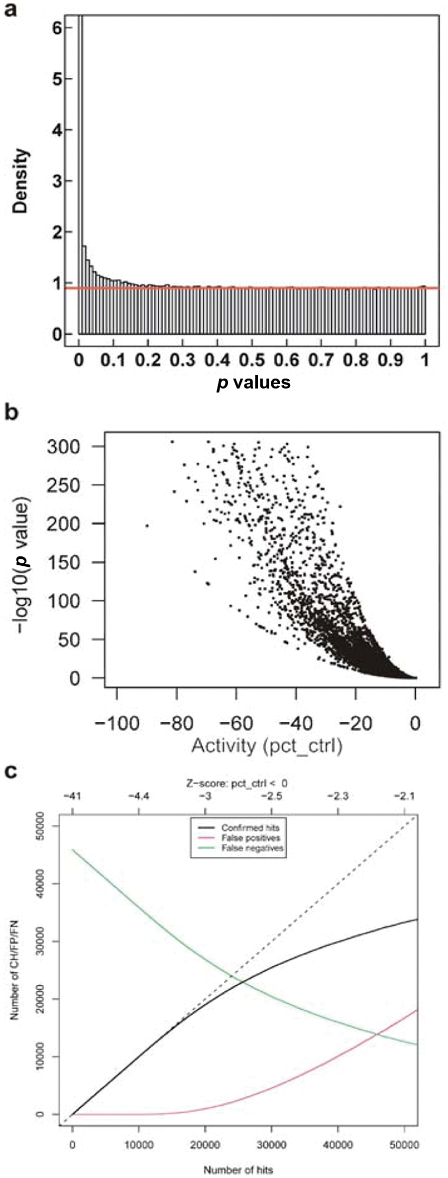
Primary screen hit selection graphs. (a) PVD with 90% inactives (red line), (b) Geyser plot (one-sided volcano plot), and (c) the cutoff selection graph displaying the number of confirmed hits as well as the number of false positives and negatives in relation to the number of selected hits, equal to the number of confirmation experiments to be performed.

From the p values and the corresponding PVD (Fig. 4a), the screening hits can be characterized as described in the methods section. Among the 549,000 compounds with activity < 0, 90% are consistent with H₀, i.e., x = 0 (they are really “inactive”). The number of confirmed hits (true positives), the number of false positives, and the number of false negatives are plotted as a function of the number of the most significant hits in Figure 4c , which are ordered by increasing p value. The graph reads, for instance, for the 40,000 most significant hits, the number of false positives is expected to be around 10,000. Up until 15,000 hits, the number of false positives is negligible and as long as the capacity for confirmation experiments is available it makes sense from a statistical point of view to retest all of them. The resulting FDR is well below 10%.

If the maximum tolerable FDR is set to 0.1%, PVDA estimates for the size of the hitlist 10,823 at a maximum p value of 2.6·10^-5 corresponding to a maximum Z-score of -4.0. Then the hitlist is predicted to include 10,158 true positives, five false positives, and exclude 415,348 true negatives, and 35,736 false negatives.

The presented graph allows for an easy but quantitative and statistically sound hit selection process, in which the experimentalist can rationally make the balance between two counteracting principles: selecting as many true hits as possible while keeping the number manageable from a logistics standpoint.

The same analysis was performed on altogether five screens of a variety of targets and assay formats from the past year. Without additional experimental efforts, the confirmation rate of primary hits in the secondary assays can be compared with the theoretical predictions from PVDA, as shown in Table 1 and Figure 5 . The agreement is very good (Wilcoxon’s signed rank test p = 0.81) and retrospectively confirms the validity of the approach.

Table 1.

Comparison of Predicted and Observed Hit ^a Confirmation Rates

Confirmation Rate, %	Screen 1	Screen 2	Screen 3	Screen 4	Screen 5
PVDA predicted	34	64	78	85	74
PVDA observed	27	69	77	88	70

a

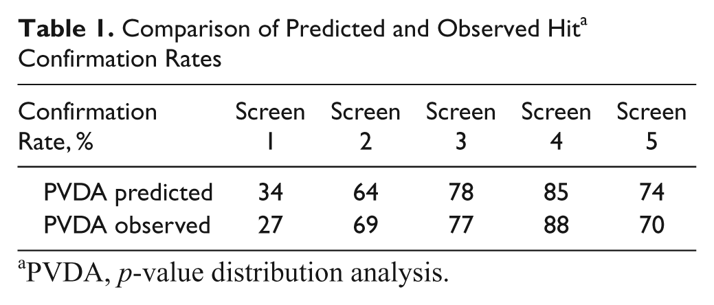
PVDA, p-value distribution analysis.

Figure 5.

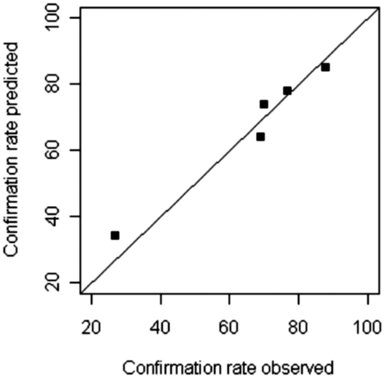
Comparison of the predicted and the experimentally determined confirmation rate for five HTS campaigns.

Discussion

The analysis of p-value distributions to control the FDR has been applied to primary compound screening hits and is reported here, to our knowledge, for the first time. In the previous sections it was described how knowledge about the activity distribution under the Null hypothesis is obtained from negative control compounds, which are present in replicates on each plate. Based on the robust estimates of location and scale of these controls under H ₀, Fisher’s Z-test is performed to calculate a p value for the single measurement of each compound. The shape of a p-value distribution of a mixture of active and inactive compounds is known and is used to derive estimates for the FPR, the FNR, and the FDR. Among them, the FDR can be readily compared to experimental confirmation results and a very good agreement is found for a variety of confirmation rates.

Distribution of Compounds and Controls

In the example shown above, and in many HTS campaigns, it is commonplace to perform pilot screens prior to the full HTS to guarantee sufficient quality, as judged by the Z′ factor. Conveniently, these data can be used to check whether the assumptions for the test statistics are fulfilled, without further experimental effort.

They also serve to learn about the assay reproducibility or the frequency of outliers, i.e., results that occur only in one out of three replicates. Too many outliers will hamper any model-based statistical analysis because the models usually do not include their presence. As a rule of thumb, when the frequency of outliers approaches the range of the hit rate statistical predictions become invalid.

Another imperfection visible in pilot experiments are trends or sudden changes in the plate-averaged signal of compounds and controls, which indicate an incorrect normalization and can make a correct statistical analysis in the worst case impossible. However, it is one main purpose of this work to present experimental evidence that even in the presence of some imperfections, predictions can be made that are valid to a large extent.

The fundamental assumption that the data are independent, identically normal distributed, is tested twofold: the distribution of all controls is normal with equal variance and the variance of the compounds is independent of the mean. For real data, in most cases, the assumption is only fulfilled approximately. Yet in fact, simulations show that the variance can increase by more than a factor of five across the whole activity range without large effect on predictions (for a uniform distribution of 0.1-1% actives, less than 15% error in the composition of the histlist; data not shown). In cases where the variance changes even more drastically, or when the type of data suggest a different error structure, monotonous transformation of the data may help to regularize the distribution, e.g., log-transform for a multiplicative error structure. ¹⁴

The two-group t-test (or Z-test) for unequal variance is not appropriate here because the p values for pooled variances are only asymptotically accurate, i.e., with an infinite number of samples. Since we are dealing here with single sample data, this is definitely not valid and would lead to irregular PVDs that cannot be analyzed with the present method.

In practice, without replicates, the Z-test is the only possible way to compute p values. But in general, PVDA is ignorant on the nature of the used test as long as the p values are correct. For this reason PVDA is easily transferable to the multivariate case. Other tests are in principle possible, for instance, the binomial test, or the signed rank test of Wilcoxon, but many require replicates and thus not applicable to single sample data. It should be emphasized that the PVDA hitlist is equivalent to the hitlist from the top-X scoring method when the variance is constant over the whole screen. But PVDA gives information on the significance and the error content of the hitlist, which are not available in the top-X method.

Parameter Estimation

After the type of test is chosen and its assumptions are checked, the parameters of the test statistics under H₀ need to be estimated. In the case of the Z-test the location and the scale of the normal distribution are estimated separately from the compound distribution using the negative controls. The reliability of this determination has a profound influence on the result of the scoring. For instance, even a MAD-based robust estimation of the variance of the H₀ distribution derived from the compound distribution (instead of the negative controls) often leads to an overestimation because the underlying assumption, that it is mostly determined by the inactive subpopulation, is not sufficiently fulfilled. Relying on a single estimate for the variance of a whole screen from the pilot experiment is also not sufficient because the variance is usually not constant. Especially between pilot screen and primary screen, due to small but important differences in the workflow timing, significant differences in the assay variability are commonly observed. It also changes during the screen along a single run due to systematic trends in the assay sensitivity coming from, e.g., decreasing enzyme activity, progressing substrate degradation/precipitation, or cell cycle-related changes in the metabolic state.

Robust estimation of the variance on each plate of the primary screen would be more appropriate to capture the day-to-day and plate-to-plate variability. In most practical cases, though, the relatively small number of controls per plate results in a large uncertainty of the variance estimation, which can lead to unnecessary false positives by an underestimation of the true variance. ¹⁴ This can be accounted for by using shrinkage methods. ¹⁶ Descriptive, simplified, and focused on the current work, shrinkage methods improve the estimation of a parameter of one group, e.g., the variance on one plate, by borrowing information from (all) other groups assuming they are in some sense similar, e.g., the plates that were measured shortly before and after. As an example, the variance of all compounds on plate i may be estimated by the weighted average of the sample variance of plate i and the variance over all controls on plates i-k to i+k without plate i, ${\tilde{\widehat{\sigma }}}_i^2=\lambda {\widehat{\sigma }}_i^2+(1-\lambda ){\widehat{\sigma }}_{2\text{k}\backslash \text{i}}^2$ the estimator ${\tilde{\widehat{\sigma }}}_i^2$ . Depending on the tuning parameter can change from ${\widehat{\sigma }}_i^2$ (local, low bias, large variance) to ${\widehat{\sigma }}_{2\text{k}\backslash \text{i}}^2$ (global, high bias, low variance). Depending on k, the estimator is more or less local. In the present work, $\lambda =\raisebox{1ex}{$1$}\!\left/ \!\raisebox{-1ex}{$2\text{K}$}\right.$ was chosen, leading to a simple averaging around plate i. The window size k was allowed to adapt for the local variability of ${\tilde{\widehat{\sigma }}}_i^2$ using a polynomial regression approach (loess), and typically ranged between 1 and 3.

Predictions from the p-Value Distribution

From the predictions made from the PVD, i.e., the FPR, FNR, and FDR, the latter can be compared with experimental results from follow-up dose-response profiling (see Table 1 and Fig. 5 ). The agreement achieved here gives confidence in the presented method, especially since the set completely represents all tried cases and no selection was made. It seems that any violation of the assumptions that may be present does not lead to large errors. This might be due to the low hit rate that is usual in HTS, and the relatively stringent cutoff at very low p values or low FDR, respectively. To gain additional confidence and to explore the range of experimental situations for which PVDA gives valid results, Monte-Carlo simulations have been performed which are described and discussed in the supplemental material. Detailed theoretical considerations may be available in the future which are both consistent with the true experimental situation and able to predict the conditions at which the approximations used here break down. However, this is beyond the scope of the present article.

Like a summary of the predictions, the gains and costs of choosing a particular number of confirmation experiments are illustrated in Figure 4b : more confirmation experiments constitute higher costs in time and reagents but bring more confirmed hits and fewer false negatives. Using a hit selection graph such as this allows the screener to find optimal conditions where the gain outweighs the cost.

The present work provides evidence that (1) p values can be accurately calculated for single-point HTS data using the variance of the controls for a Z-test, and that (2) from the p-value distribution, the relevant screen characteristics can be estimated. Most prominently, the false discovery rate allows prediction of the expected hit confirmation rate prior to any follow-up experiment.

Several advantages compared with the most widely used hit-list generation method, the topX method can be mentioned: PVDA allows finding out whether a candidate list contains any statistically significant hit at all. Especially screens with very few active compounds or with very weak compounds or large assay variability may have very few significant hits but will always have a top 100 list. A quick look at the PVD whether a peak at low p values is visible gives a qualitative impression about the expected FDR of the hit list.

The cutoff selection according to a preset false-discovery rate is among the most transparent rules and easy to interpret. In addition, by estimating the plate-wise variance, any variation of the assay variability from plate to plate is taken into account. And in situations where the calculated p values are not exact, the shape of the p-value distribution allows for an easy internal quality control. The essence of the method is finally illustrated by the relation of gains and costs of choosing a particular hit list size.

With PVDA, a modern and powerful statistical method was applied to HTS data. In the future, with more academic groups embarking on the journey of high-throughput miniaturized assays, both for genome-wide siRNA screens and small molecule compound screens, we expect new and more tailor-made methods to be developed which will enable an even better and scientifically sound analysis of large data sets.