
Abstract
Superior corporate environmental performance (CEP) is considered to be an indication of well-managed firms. While previous empirical research has operationalized various environmental measurements, one aspect has remained under-scrutinized, namely, continuous improvement. We examine whether continuous CEP improvement is reflected in aggregated environmental scores provided by sustainability rating agencies. From a natural resource-based view, we investigate the association of continuous CEP improvement with corporate financial performance (CFP). Based on panel data (2005–2020), the results show that continuous CEP improvement is not associated with aggregated environmental scores provided by three major rating agencies. At the same time, however, continuous improvement is positively associated with accounting as well as market-based CFP. The article concludes that continuous CEP improvement is relevant from a materiality perspective, but it is not adequately captured in the environmental scores from rating agencies. Therefore, we propose using a best-in-progress approach as a meaningful investment strategy instead of the established best-in-class screenings.
Keywords
Introduction
In academic research on organizations and the natural environment, corporate environmental performance (CEP) is seen as a multidimensional construct, which can be separated into the description of implemented processes and the realized outcomes that these processes generate (Delmas et al., 2013; Misani & Pogutz, 2015; Trumpp et al., 2015). Relatedly, several authors use corresponding terms, including environmental management performance relating to process-based measures (Ilinitch et al., 1998; Jung et al., 2001) and environmental operational performance relating to outcome-based measures (Trumpp et al., 2015). This article focuses on the latter aspect, the environmental outcomes from operational activities. To measure corporate performance from this operational perspective, indicators for physical inputs and outputs can be utilized (Jung et al., 2001; Shrivastava, 1995). These indicators can be operationalized in three distinct ways: annually as raw performance data, annually as improvement ratios, and as continuous improvement (Hart, 1995) over time. In this article, we seek to make a novel contribution with empirical results to the third approach, namely, continuous CEP improvement.
While research considering natural resource-based perspectives and proactive environmental strategies has emphasized the importance of continuous improvement as an organizational capability (Hart, 1995; Sharma & Vredenburg, 1998; Surroca et al., 2010), no previous study has empirically investigated CEP as a continuous improvement. Continuous improvement is defined in this article as a “recurring activity to enhance performance” (ISO, 2015). The majority of the empirical research measures CEP based on annual raw performance data. For example, many studies examine the relationship between CEP for a given year and corporate financial performance (CFP) in the following year (Grewatsch & Kleindienst, 2017; Hang et al., 2019). A few studies focus on change-related properties of CEP and investigate improvement ratios, such as realized reductions in carbon emissions (Delmas et al., 2015; Lewandowski, 2017; Misani & Pogutz, 2015) or toxic waste (Berchicci et al., 2012, 2017). For example, Berchicci et al. (2017) investigate the positive spillover effects and find that facilities improve CEP after acquisition. However, no previous study has empirically investigated the relevance of continuous CEP improvement over multiple years. As such, this article is essential in providing a new perspective on measuring and interpreting CEP. Static representations of CEP do not inform us of whether organizations are continually improving—an essential requirement for tracking substantial progress over time. In the context of climate change, for example, it is important for managers and investors to monitor if companies are achieving continual, absolute greenhouse gas (GHG) emission reductions year after year.
To shed light on this relevance of dynamic considerations, we formulate two research questions:
We use panel data from four different sustainability rating agencies, including Thomson Reuters Asset4, ISS-oekom, MSCI ESG IVA, and KLD, covering the years from 2005 to 2020. To measure continuous CEP improvement in an adequate manner, we first collect data on outcome-based indicators at the firm level, including physical inputs (i.e., total energy use and total water use) and physical outputs (i.e., total CO2 equivalent emissions and total water discharge). Based on this, we are able to develop two measurements for continuous CEP improvement in each firm: the cumulative improvement effect and the annual improvement rate over the entire period.
Our results reveal that continuous CEP improvement is not associated with aggregated environmental scores from sustainability ratings in a meaningful way. This holds true for the environment scores provided by all three sustainable rating agencies in our sample. We also confirm this result for KLD data in a robustness check. At the same time, our results show that all indicators of continuous CEP improvement are highly relevant from a materiality point of view, as all CEP indicators are positively associated with CFP (i.e., return on assets [ROA] and Tobin’s q).
This study contributes to the organizations and natural environment literature in several ways. First, we contribute to this literature by conceptually deriving a measurement approach for continuous CEP improvement and empirically testing it. While previous studies have captured change-related aspects of CEP based on the annual changes between 2 years (e.g., Alvarez, 2012; Ortiz-de-Mandojana & Bansal, 2016), this is the first study that reflects continuous improvement over many years. Based on two novel measurements, we are able to empirically validate that continuous CEP improvement is an important organizational capability. This holds not only for environmental outcomes but also from a financial perspective as depicted by the natural resource-based view (Branco & Rodrigues, 2006; Hart, 1995; Russo & Fouts, 1997). As such, our findings complement the extant CEP–CFP research by showing that through continuous CEP improvement, physical inputs are saved and physical outputs are prevented, which, in turn, yields increased internal profitability and heightened investor confidence (Delmas et al., 2015; Hang et al., 2019).
Second, the validity and consistency of aggregated scores provided by sustainability rating agencies have been the focus of many recent studies (Berg et al., 2019; Chatterji et al., 2016; Eccles et al., 2019). We are able to contribute to this literature by demonstrating that continuous CEP improvement is not adequately reflected in aggregated environmental scores provided by sustainability ratings, including ISS-oekom, MSCI ESG IVA, and KLD. This finding highlights that continuously improving CEP on the operational level does not automatically factor into the aggregated environmental scores of sustainability ratings. This is an interesting finding as previous research has found that superior environmental processes are positively correlated to environmental outcomes and together can explain a major proportion of variation in aggregated environmental scores (Delmas et al., 2013). Furthermore, rating agencies disclose that environmental outcomes are a major component in the construction of the aggregated environmental scores (Misani & Pogutz, 2015). While this may be the case for annual performance data to some extent, our results reveal that the environmental scores do not reflect continuous CEP improvement in a meaningful way.
Third, taking the practitioner’s point of view, our results have major implications for sustainability-oriented investors. Many investors rely on the so-called “best-in-class” approach, which limits the investment universe to those firms that have superior sustainability ratings within a sector (Global Sustainable Investment Alliance [GSIA], 2021). If a best-in-class approach based on aggregated environmental scores was effective in capturing the main CEP aspects, that is, environmental processes and outcomes, we would expect continuous improvement to be reflected in these scores. We discover, however, that these scores do not capture superior environmental performance based on continuous CEP improvement. As such, best-in-class screenings cannot fulfill this purpose. If investors seek to identify companies that in fact improve their CEP outcomes, they should apply a best-in-progress approach. At the same time, this approach also makes sense from a materiality point of view: our results reveal that continuous CEP improvement has a highly positive association with CFP. Thus, managers, investors, and academics alike should also reflect on continuous improvement from a best-in-progress approach for a more holistic assessment of CEP.
Literature Review
Multidimensionality of CEP
CEP is a multidimensional construct with distinct, albeit interrelated, aspects. This implies, in turn, that the literature faces the issue of conceptual ambiguity (Suddaby, 2010). According to the ISO 14031 definition (ISO, 2015), a norm for environmental performance evaluation, CEP is defined as “measurable results of an organization’s management of its environmental aspects.” While this definition delivers conceptual clarity regarding a common understanding, the operationalization of CEP remains under the discretion of the investigator (i.e., academic researcher, investment analyst, etc.).
Several authors have classified various elements as dimensions of CEP. Ilinitch et al. (1998) proposed multiple categories of CEP based on two generic dimensions—processes and outcomes. According to them (ibid.), internal systems belong to process-related aspects, and environmental impacts can be considered outcome-related issues. Trumpp et al. (2015) rephrased these dimensions as environmental management performance (EMP) and environmental operational performance (EOP). EMP is process-related, and it contains the “strategic level of environmental performance and focuses on management principles and activities with regard to the natural environment” (Trumpp et al., 2015, p. 190). EOP is outcome-related, and it includes “the environmental impacts of a firm’s management activities regarding the natural environment” (ibid.). Accordingly, outcome-based indicators related to operational performance are based on physical inputs and outputs (Jung et al., 2001; Shrivastava, 1995). Typically, these indicators either use the absolute performance value for a given year or they are expressed in relative terms, that is, as intensity by dividing the absolute value by sales (Hoffman & Busch, 2008).
The availability and quality of corporate environmental data have improved over the years, and CEP has been observable in academic studies on the operational level for several decades (Trumpp et al., 2015). Key sources of outcome-based data are mandatory reporting schemes from governmental agencies, such as the Toxic Release Inventory (TRI; for example, Chatterji et al., 2009; King & Lenox, 2002), as well as voluntary reporting schemes from nongovernmental agencies, such as the CDP (formerly known as the Carbon Disclosure Project; for example, Misani & Pogutz, 2015) and the Global Reporting Initiative (GRI). Furthermore, many studies incorporate CEP data offered by third-party providers, including Bloomberg, ISS-oekom, MSCI, Sustainalytics, Thomson Reuters, and Trucost.
These providers offer proprietary data on companies’ environmental, social, and governance criteria (e.g., Cheng et al., 2014; Escrig-Olmedo et al., 2017), covering a range of raw data on an annual basis, from disaggregated data points on environmental outcomes (e.g., total energy use, emissions, etc.) to aggregated environmental scores. As a result, several studies have incorporated outcome-based indicators based on physical inputs such as energy or water use and outputs such as emissions or waste (e.g., Delmas et al., 2015; Lewandowski, 2017; Misani & Pogutz, 2015).
Operationalization of Outcome-Based CEP
When investigating the relationship between CEP and other firm-based performance measures, such as CFP, outcome-based indicators can be operationalized in three distinct ways: annually as raw performance data, annually as improvement figures and ratios, and as continuous improvement over time. First, a good portion of early empirical research on CEP was based on annual raw performance data expressed in absolute or relative terms (e.g., King & Lenox, 2002; Wagner, 2005). These studies observe the environmental performance level of a firm for 1 year and put it in context with other measures of firm performance. While many early studies in this realm used cross-sectional data for a given single year, many more recent studies utilize panel data (e.g., Wagner, 2005). While these studies capture the general relevance of CEP for other measures of firm performance, they do not reveal any information about the relevance of CEP improvement (Elsayed & Paton, 2005; Wagner, 2005).
The notion of CEP improvement has been incorporated into recent studies. Several studies have focused on change-related properties of CEP and have investigated improvement ratios (e.g., Berchicci et al., 2012, 2017; Delmas et al., 2015; Lewandowski, 2017). These studies have acknowledged that the dynamic properties of CEP have been mentioned in earlier conceptual papers (e.g., Hart, 1995; Hart & Milstein, 2003) and deliver corresponding empirical evaluations (Short et al., 2016). These studies have operationalized the change-related properties of CEP in different ways, either as a change in facilities’ waste generation (Berchicci et al., 2017), as a decrease in firms’ emissions (Alvarez, 2012; Delmas et al., 2015; Lewandowski, 2017), or as an improvement of firms’ aggregated environmental scores (Ruf et al., 2001; Yadav et al., 2017).
Several studies have conceptualized what managers could measure in terms of continuous improvement, that is, operational performance indicators such as energy use or carbon emissions (e.g., Albertini, 2013; Brouwer & van Koppen, 2008). Yet, no study has operationalized empirical data to investigate the association between continuous CEP improvement and other key measures of firm performance, such as CFP. For this reason, we develop two novel approaches to operationalize continuous CEP improvement and derive related hypotheses.
Theoretical Framework and Hypotheses Development
Continuous Improvement as an Organizational Capability
The notion of continuous improvement originates in the total quality management literature (Deming, 1982) and has proliferated through developments of well-recognized management initiatives, such as lean production and Six Sigma (Anand et al., 2009; Sanchez & Blanco, 2014). Continuous improvement entails a firm’s ability to plan, implement, and work toward the goal “to correct the cause not the symptoms . . . and so effect permanent improvement” (Bond, 1999, p. 1320). As many organizational fields become increasingly complex and experience rapid technological changes, firms rely on their capability to improve their existing processes, products, services, and performance on a continuous basis (Anand et al., 2009). As the concept of continuous improvement implies, firms are frequently and deliberately adjusting their processes over longer periods, and it has been noted that “organizations that use this process focus on making small, incremental changes, modifying them, and eventually creating a large, cumulative effect” (Choi, 1995, p. 612).
From the literature on organizations and the natural environment, continuous improvement has been considered to be a key organizational capability to increase resource efficiency and reduce environmental impacts over time (Brouwer & van Koppen, 2008; Sharma & Vredenburg, 1998). The natural resource-based view proposes that firms seeking continuous improvement should continuously innovate and seek ways to reduce their environmental impact, such as preventing pollution (Albertini, 2013; Hart, 1995; Sharma & Vredenburg, 1998). According to international environmental standards, especially the ISO 14001 environmental management norm, continuous CEP improvement is considered a key component of superior environmental performance (Brouwer & van Koppen, 2008). The resource-based view also posits that companies are considered “a bundle of strategic and operating resources . . . represented as a set of visions, inputs, throughputs, and outputs (VITO)” (Shrivastava, 1995, p. 189). In this way, environmental improvements on an operational level can be broken down into physical inputs and physical outputs (Jung et al., 2001). As such, the next two subsections discuss the relevance of continuous CEP improvement on the operational level in more depth and derive our hypotheses.
Continuous CEP Improvement and Aggregated Environmental Scores
Due to the rising demand for sustainability-related investment products over the last decade, a significant interest in reliable environmental data has emerged (Chatterji et al., 2009; Delmas et al., 2013; Eccles et al., 2019). This has led to the expansion of environmental data offered by sustainability rating agencies and data providers, such as Asset4, MSCI, RobecoSAM, Sustainalytics, and KLD (Berg et al., 2019; Eccles et al., 2019; Mattingly & Berman, 2006). Another recent phenomenon is that major established financial data providers have acquired sustainability rating agencies, and now offer ratings on firms’ social and environmental performance, that is, Bloomberg, ISS-oekom, and MSCI (Eccles et al., 2019).
Previous studies recognized a need for sustainability rating agencies to develop consistent and comprehensive scores for measuring firms’ environmental performance (Escrig-Olmedo et al., 2017; Singh et al., 2009). While aggregated environmental scores cover multiple environmental dimensions, we see two reasons why continuous CEP improvement should be expected to be adequately reflected by aggregated environmental scores. First, Trumpp et al. (2015) reveal that superior environmental management (i.e., process-based environmental indicators) is positively associated with high levels of environmental operational performance (i.e., outcome-based environmental indicators). As continuous improvement in environmental outcomes is the result of corporate strategy and previously implemented superior environmental policies (Jiang & Bansal, 2003), we assume environmental processes and outcomes to be positively correlated. This implies, in turn, that continuous CEP improvement should be reflected in high environmental scores (Dragomir, 2018).
Second, it has been empirically validated that operational performance (outcome-based indicators) along with environmental management (process-based indicators) represent a good portion of variation in aggregated environmental scores (Delmas et al., 2013; Misani & Pogutz, 2015). Rating agencies, such as ISS-oekom and MSCI, state that outcome-based indicators related to physical inputs and outputs play an important role in the construction of these aggregated scores (Misani & Pogutz, 2015). This implies that continuously improved environmental outcomes should factor into high environmental scores. Thus, we propose the following hypothesis:
Continuous CEP Improvement and CFP
An ongoing inquiry as to whether and under what circumstances it pays to be green can be traced back to the 1970s (Grewatsch & Kleindienst, 2017). The majority of studies draws the conclusion that CEP does not have a negative association with CFP (Friede et al., 2015; Russo & Minto, 2012), while many studies find that CEP positively influences CFP (e.g., Delmas et al., 2015; Hang et al., 2019). One important conclusion in this realm may be that the link between environmental strategy and competitive advantage depends on the form of environmental improvement being considered . . . being committed to pollution prevention is less likely to create profit by itself, than when it is in combination with general capabilities (Albertini, 2013, p. 435).
Building upon the natural resource-based view (Aragón-Correa & Sharma, 2003; Hart, 1995; Russo & Fouts, 1997), continuous improvement is considered one of these important organizational capabilities, which can lead to the achievement of simultaneous economic and environmental benefits through reflection and organizational learning (Albertini, 2013; Nonet et al., 2016; Sharma & Vredenburg, 1998). Companies possessing the capability for continuous CEP improvement focus on well-defined environmental objectives rather than merely on “end-of-pipe” solutions (Hart, 1995), which tend to be very costly. In this sense, continuous improvement helps firms to concentrate on eradicating the root cause of the problem rather than merely the symptoms (Bond, 1999; Hart & Milstein, 2003; Sharma & Vredenburg, 1998). Several studies have shown that companies possessing the capability for continuous improvement experience lower investment and implementation costs for environmentally friendly technologies (Brouwer & van Koppen, 2008; Hart & Milstein, 2003).
From a physical input perspective (Shrivastava, 1995), a reduction in material and energy consumption corresponds to an increase in resource efficiency and productivity (Aragón-Correa & Sharma, 2003; Hart & Dowell, 2011; Hart & Milstein, 2003). Resource efficiency is a central term used in the assessment of environmental performance, as it seeks to decouple the direct relation between business growth, natural resource exploitation, and environmental degradation (Trumpp et al., 2015). More efficient use of natural resources and energy directly affects operational costs, and thus, should enhance accounting-based CFP.
From a physical output perspective (Shrivastava, 1995), the reduction in environmental outputs, such as emissions, water discharge, or waste, can create competitive benefits. These stem from cost savings through internal waste prevention to monetary benefits for lowering carbon emission levels from carbon trading schemes (Busch & Hoffmann, 2011; Cadez et al., 2019). For example, several authors find clear evidence that waste management contributes to a financial benefit over mere waste reduction (King & Lenox, 2002), as onsite treatment is associated with high investment costs and even increased waste amounts, as these amounts are correctly accounted for the first time. As physical outputs have a direct effect on the cost structure of firms, we predict that optimizations will be positively associated with accounting-based CFP.
Financial benefits achieved through superior CEP can encourage companies to reinvest in further CEP improvements, which is called the virtuous circle (Waddock & Graves, 1997). Presuming that such efforts are recognized and valued by financial market participants, such gained operational efficiencies should also be reflected in market-based CFP. Furthermore, profitability from improved CEP can lead to further spillover effects for market-based indicators, including increased investor confidence and an improved reputation with stakeholders (Hart & Dowell, 2011; Lewandowski, 2017). For example, several authors claim that investors perceive superior carbon performance as a top value, as low-carbon companies may provide a “carbon premium” (Busch & Hoffmann, 2011; Misani & Pogutz, 2015). Therefore, the second hypothesis is framed as follows:
The next section describes the method, including how the samples were generated to test the hypotheses, and how the data was collected and operationalized.
Method
Data Collection
To estimate our panel regression models, we draw data from various sources, including Thomson Reuters Asset4, ISS-oekom, MSCI ESG Intangible Value Assessment (IVA), and Compustat. We collect longitudinal data on various environmental and financial aspects for the timeframe 2005–2020. Thomson Reuters Asset4 (2017) offers a range of variables for environmental performance, ranging from disaggregated raw data points to aggregated environmental scores. According to Trumpp et al. (2015, p. 192), Asset4 is the only “available database that provides non-aggregated data” for numerous process-based and outcome-based environmental indicators. In a first step, we search for adequate disaggregate indicators in Asset4 that best capture environmental outcomes, including physical inputs and outputs. Afterward, we include four disaggregate indicators that have considerable firm-year observations for our panel data regressions, including (a) total energy use and (b) total water use as physical input indicators, and (c) total CO2 equivalent emissions (Scope 1 and 2), and (d) total water discharge as physical output indicators. Despite the fact that several authors considered waste to be an important environmental output indicator (Brouwer & van Koppen, 2008; Trumpp et al., 2015), we excluded this indicator due to a lack of data availability.
For the aggregated environmental scores, we collect data from ISS-oekom, MSCI ESG IVA, and MSCI KLD. Each of these databases provides an aggregated environmental score separated from other sustainability issues, such as social and governance. The MSCI KLD environmental scores are only used in a robustness check. While KLD data are considered a “widely recognized benchmark for measuring the impact of [. . .] environmental screening on investment portfolios” (Ortiz-de-Mandojana & Bansal, 2016, p. 37), many studies pointed toward issues concerning aggregation issues, notably when aggregating KLD strengths and concerns (e.g., Berg et al., 2019; Escrig-Olmedo et al., 2017).
We collect all financial data from Compustat, including total annual sales, total assets, total equity, total liabilities, R&D expenditures, cashflow, and market capitalization to calculate ROA and Tobin’s q.
Data Description
Our total sample covers up to 1,724 companies totaling 9,759 firm-year observations for the period 2005–2020. The panel is unbalanced because, depending on data availability, separate models have smaller observations. Therefore, we conduct t-tests to assess the differences between the means of the individual models and our total sample. Supported by a large number of firm-year observations, we cannot find that the means significantly differed between any of our models (95% confidence interval). In addition, similar to previous studies (Trumpp & Guenther, 2017), we use the winsorizing technique at the top and bottom first percentiles for all variables used in this study to account for potential outliers in the dataset. The following sections describe the dependent, independent, and control variables.
Dependent Variables
To test our first hypothesis, we obtain aggregated environmental scores from ISS-oekom and MSCI ESG IVA. In our sample, ISS-oekom provides environmental scores for more than 1,800 companies in 120 countries. Their rating scale is translated into units that allow for the computation of environmental scores (ISS-oekom, 2018). Finally, MSCI ESG IVA provides scores for more than 1,500 global firms in our sample. Their environmental performance is on a scale from 0 to 10, which is based on the categories climate change, natural capital, pollution and waste, and environmental opportunities (MSCI, 2014). These two environmental scores are acceptable for our empirical analysis, as they aggregate environmental characteristics of the firm and claim to include outcome-based indicators in their rating of firms’ environmental performance (Eccles et al., 2019; Misani & Pogutz, 2015).
To test the second hypothesis, we obtain financial data from Compustat, including net income as well as total assets, total equity, total liabilities, and market capitalization to calculate ROA and Tobin’s q. These financial variables are frequently used in the literature researching the connection between CEP and CFP. For example, several prominent studies (Delmas et al., 2015; King & Lenox, 2002; Russo & Fouts, 1997) use ROA and Tobin’s q exclusively to depict companies’ financial performance. Thus, we include measures for accounting-based CFP portrayed as ROA as well as market-based CFP portrayed as Tobin’s q to capture a firm’s financial performance. ROA gives a manager, investor, or analyst an idea of how efficient a company’s management is at using its assets to generate earnings. Tobin’s q is calculated as the market value of a company divided by the replacement value of the firm’s assets.
Independent Variables
Our longitudinal dataset allows us to capture the improvement in disaggregated CEP measures. For the disaggregated variables, we use annual sales figures to determine the intensity of the respective environmental variables (e.g., total energy use divided by total annual sales) and then calculate the dynamic factor ΔCEP as a year-over-year percentage change in intensity, which is similar to several previous studies (Alvarez, 2012; Lewandowski, 2017). Figure 1 depicts our calculation measuring annual CEP improvement. To illustrate our ΔCEP calculation, we provide an example: we subtract a company’s previous year’s carbon intensity (CO2/Sales t − 1) from the current year’s data (CO2/Sales t), divided by the previous year’s intensity (CO2/Sales t-1). As we are assessing improvements year after year, a decrease in intensity will result in a positive coefficient value.
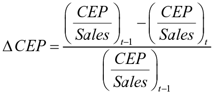
Calculation for CEP Annual Improvement (ΔCEP)
We use intensities for these disaggregated environmental variables, as these relative terms allow us to compare the effects for companies of different sizes and correct for pure growth effects. To illustrate our variable design, the average carbon intensity of our sample is 0.02. This implies that—on average—a company with US$25,000,000 sales would emit 500,000t of CO2 equivalents. If sales stay the same while the company improves its carbon intensity by one percent, the company’s CO2 equivalent emissions would be reduced by 5,000t.
After calculating the year-over-year percentage change for each intensity variable, we operationalize the data to capture continuous improvement. First, we introduce a persistence measure for continuous CEP improvement over multiple years, which we have labeled the cumulative improvement effect. The calculation of the variable is based on the accumulative years that a firm has experienced an improvement. For example, if a company improved consecutively in the timeframe 2005–2010 (5 years) but did not improve at all between 2011 and 2016, and then improved consecutively again in the timeframe 2017–2020 (4 years), we consider the cumulative improvement effect to equal nine in the final calculation. We present this cumulative improvement effect variable along with the ΔCEP in certain models (see Tables 2, 3, and 6 in the Findings).
Second, we present an amplitude measure for continuous improvement, which we have labeled the average improvement rate. This approach is inspired by the literature on the compound annual growth rate, which provides a smooth, constant rate of return over the entire time period (Chan, 2009). To calculate the average improvement rate, we divide the initial value by the end value for each firm, and then take the square root of the fraction of 1 over the number of years. Figure 2 portrays the calculation of the average improvement rate for our independent variables.
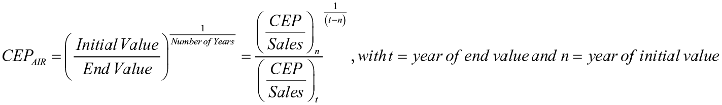
Calculation for CEP Average Improvement Rate (CEP_AIR)
The initial value will be the year with the first documented CEP intensity per firm, and it will remain the initial value over all periods. The end value will change correspondingly depending on the year of interest. For example, if a company has published information on their CO2-equivalent emissions for the first time in 2007, we will accordingly calculate the carbon intensity for 2007 as the initial value. The end value will change from year to year. In 2008, the end value will be based on the carbon intensity for this year, and in 2009, the end value will be based on the carbon intensity in 2009 and so on. Thereafter, the average improvement rate will be calculated over the respective timeframe. This variable is presented separately from the cumulative improvement effect in certain models (see Tables 4, 5, and 7 in the Findings).
Control Variables
There are a number of control variables that are likely to be associated with our dependent variables. Risk has been considered a source of firm-level heterogeneity in previous studies (e.g., Delmas et al., 2015), and it is included as a control variable, calculated as the debt to assets ratio. In addition, we consider firm size to affect financial performance and therefore include it in the form of a logarithm of total assets (log[assets]). We also include R&D intensity (i.e., R&D divided by sales) as a control, as it has been argued in the literature that distinctive technological capabilities can create value for firms (Barnett & Salomon, 2012; McWilliams & Siegel, 2000; Shrivastava, 1995) and thus can have an effect on CFP. In addition, we control for capital intensity and cash flow in our regression models to capture a firm’s investments in growth opportunities and financial liquidity (Delmas et al., 2015; Trumpp & Guenther, 2017). As environmental improvement necessitates upfront financial investments on the part of the firm (i.e., new equipment, consultancies, and training), which are not entirely offset by financial returns from environmental activities (Hang et al., 2019), negative consequences are more likely to occur in the short term, when the costs are incurred. Similar to other studies (e.g., Lewandowski, 2017), we did not use the logarithm for cash flow.
Statistical Analysis
According to our two hypotheses, we analyze the relevance of continuous CEP improvement in two different ways: (a) its association with aggregated environmental scores and (b) its association with CFP. According to our first research question, we model the relationship between aggregated environmental scores and continuous improvement of disaggregated environmental variables as follows:
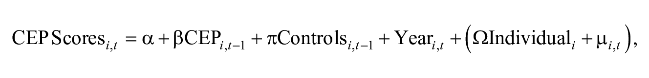
where time is denoted by t and firms are denoted by i. CEP Scores is our dependent variable (i.e., either the rating obtained from ISS-oekom or MSCI). CEP is our explanatory variable, which is integrated in two ways: first, as the cumulative improvement effect measured as the change between 2 years (ΔCEP) plus the count variable for improvement over the years (ΔCEP_cumulative), and second, as the average improvement rate (CEP_AIR). As the environmental scores from rating agencies are based on the previous year’s performance, the observations for the main explanatory variables (e.g., ΔCEP variables) and control variables are lagged 1 year behind for testing H1. Individual represents firm-fixed effects, which control for firm unobserved heterogeneity that captures any time-invariant firm characteristics. In all models, we also use year-fixed effects to denote time effects that capture common shocks, like financial crises, changes in government policy, or other systematic macroeconomic shocks that affect the financial performance of all firms. µ is the error term that captures all other omitted factors. As environment scores may be influenced by previous environmental performance, we included the previous CEP scores in the models.
Next, we consider the association of continuous improvement of disaggregated environmental indicators with CFP and modified the econometric model accordingly:

Again, time is denoted by t and firms are denoted by i. Here, CFP is our dependent variable, including ROA and Tobin’s q. In this case, we again present CEP in two ways, the cumulative improvement effect and the average improvement rate, for all disaggregate environmental indicators: Energy, Water, CO2, and WaterDischarge. For the controls, we include Risk, Size, Capital Intensity, Cashflow, and R&D Intensity. To rule out issues of endogeneity, we lag all independent variables that do not indicate annual change rates as prior research has suggested (Russo & Fouts, 1997). In addition, we include lagged dependent variables as control variables—that is, lagged ROA and Tobin’s q (Barnett & Salomon, 2012; Surroca et al., 2010). Other CEP studies lag the main explanatory variables, that is, the logarithm of total GHG emissions (Delmas et al., 2015) and the difference between logarithms of actual and predicted waste (King & Lenox, 2002); however, we decided against this for several reasons. First, our measure of continuous CEP improvement rates already includes prior year data in their formulae. As a result, the difference between 2 years builds a time interval into the measurement. Second, we believe that lagging the main explanatory variables behind the dependent variables by 1 year could cause misspecification. We intend to examine the effects of achieved continuous CEP improvements on the operating expenses. This effect will be tangible on the profit and loss statement in that very year—as such the effect will also be displayed in accounting-based CFP. If we took the ROA of the next year instead of the concurrent year, then other factors—that occur in the future—could affect the ROA figure as well. For Tobin’s q we see a similar reason. We presume that improved internal operational efficiencies from continuous CEP will result in additional spillover effects for market-based indicators, such as increased investor confidence (Hart & Dowell, 2011; Lewandowski, 2017). If we investigated the effect on Tobin’s q 1 year ahead, it is quite plausible that new, nonrelated information could alter the market value, which could potentially counterbalance the main effect.
For all basic models, we start with a pooled ordinary least squares (OLS) model, which is consistent and efficient if individual heterogeneity is not expected (or Individual only contains a constant term). In contrast, both random effects and fixed effects assume the existence of unobserved individual heterogeneity (Individual), with fixed effects models allowing for correlation between Individual and CEP or Control, whereas random-effects models do not allow for this correlation. Thus, if Individual is uncorrelated with CEP or Control, random effects will be more efficient, while if Individual is correlated with CEP or Control, random effects will be biased but fixed effects will be consistent.
In addition, we conduct the Breusch-Pagan Lagrange Multiplier (LM) test to decide between a random effect or pooled OLS regression. The LM test has a null hypothesis of zero variances across individuals. To decide between random and fixed effects, we run a Hausman test with a null hypothesis of µ it not correlated with other control variables (CEP or Control). Our test results show that fixed effects are the most appropriate econometric model. We use standard errors that are robust to heteroscedasticity and serial correlation in all fixed effects models.
Results
Descriptive Statistics
Table 1 presents the descriptive statistics for the underlying set of variables. For all ΔCEP variables, the values are close to zero, indicating an even distribution between companies increasing and decreasing their environmental performance over the entire sample. All variables appear to be within a reasonable range of variation. For ROA, we find a mean value of 4.5%, while the mean value of Tobin’s q is slightly greater than 1. This indicates that, on average, the market value of companies is marginally higher than the disclosed value of assets.
Descriptive Statistics and Correlations.
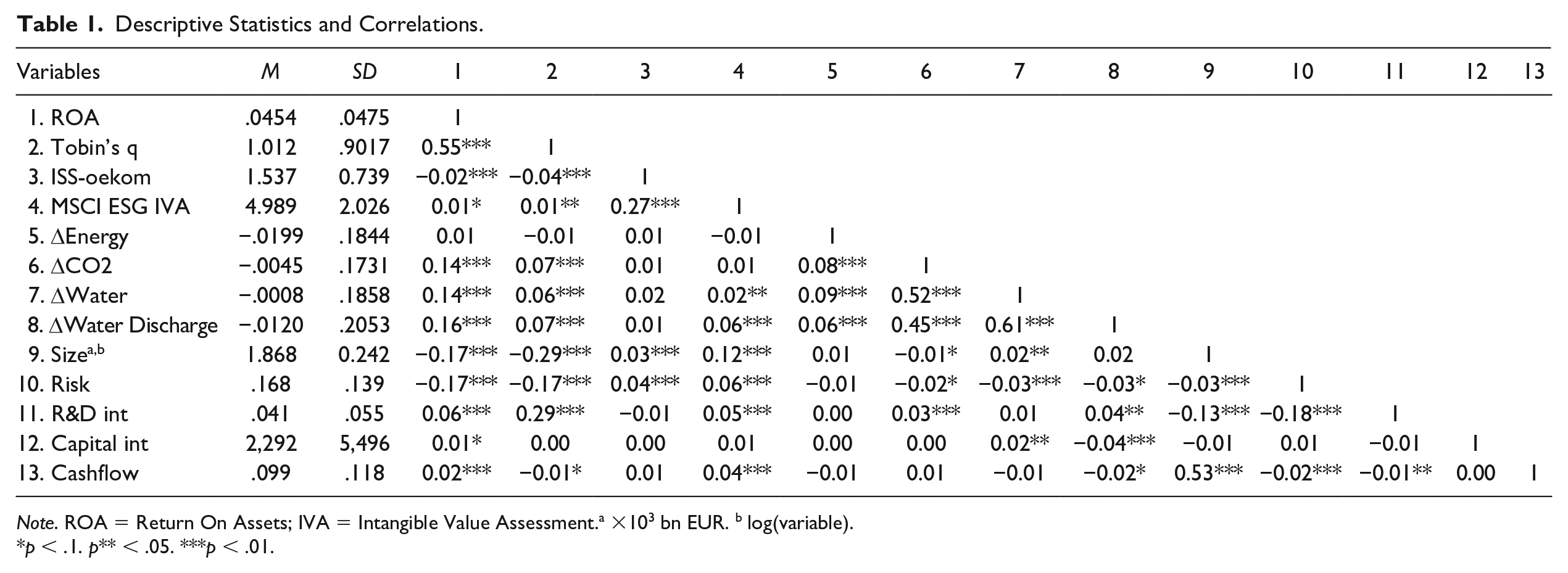
Note. ROA = Return On Assets; IVA = Intangible Value Assessment.a ×103 bn EUR. b log(variable).
p < .1. p** < .05. ***p < .01.
In addition, we detect that most variables are only slightly correlated with each other. For the ΔCEP variables, we see that, that is, ΔEnergy is not strongly correlated with ΔCO2 (0.08) and that ΔWater is only moderately correlated with ΔWaterDischarge at 0.61. Using the Variance Inflation Factor (VIF), we tested if the inclusion of all ΔCEP variables in the model is possible. The test indicated that there are no problematic issues with multicollinearity (i.e., the VIF values ranged from 1.01 to 2.07, which is well below the commonly accepted threshold of 10; Neter et al., 1996). As a result, we integrate all CEP variables into multiple models for both hypotheses.
Main Results
For H1, we provide four tables consisting of eight models each for both aggregated CEP Scores (i.e., ISS-oekom and MSCI ESG IVA) and our disaggregated CEP variables, represented in two measurements for continuous CEP improvement (i.e., the cumulative improvement effect measured by ΔCEP & ΔCEP_cumulative) and the average improvement rate (CEP_AIR). We adhere to a consistent pattern to present our results. We start with the cumulative improvement effect for both CEP Scores, including ISS-oekom (Table 2 including Models 1–10) and MSCI ESG IVA (Table 3 including Models 11–20). Next, we present the results for the average improvement rate and both aggregated CEP Scores, including ISS-oekom (Table 4 including Models 21–30), and MSCI ESG IVA (Table 5 including Models 31–40). In all tables, the four disaggregate measures are presented in the same sequence: CO2, Energy, Water, and WaterDischarge.
Regression Results for CEP Cumulative Improvement Effect and ISS-oekom Environmental Score.
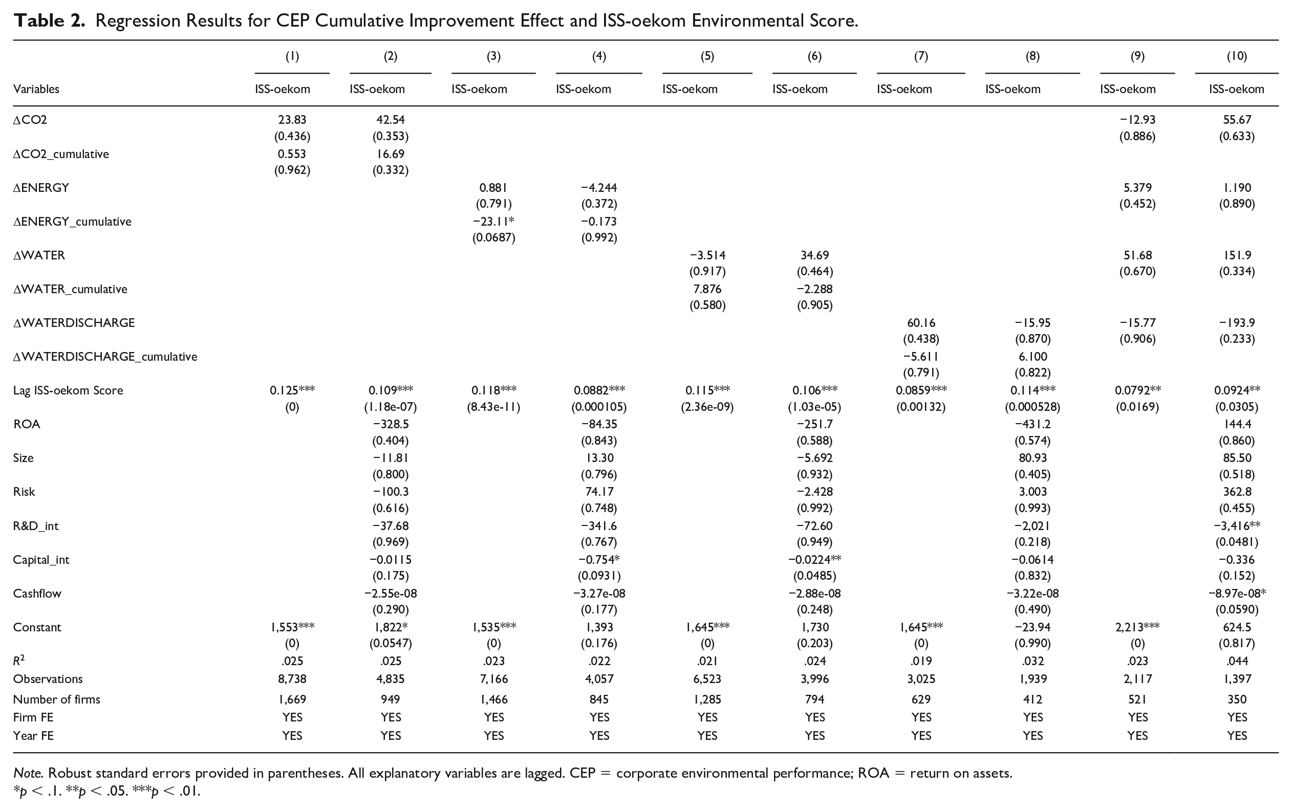
Note. Robust standard errors provided in parentheses. All explanatory variables are lagged. CEP = corporate environmental performance; ROA = return on assets.
p < .1. **p < .05. ***p < .01.
Regression Results for CEP Cumulative Improvement Effect and MSCI ESG IVA Environmental Score.
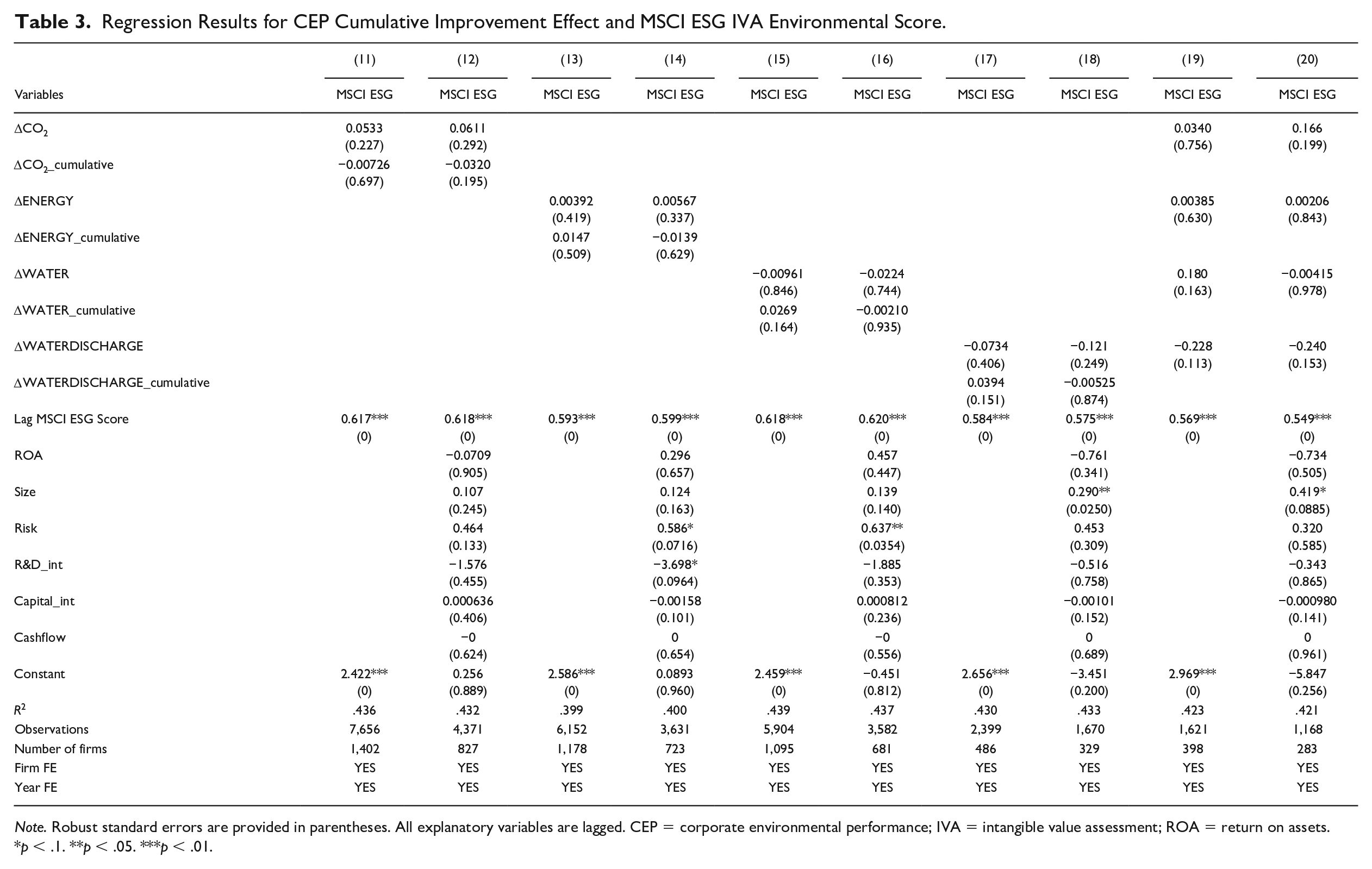
Note. Robust standard errors are provided in parentheses. All explanatory variables are lagged. CEP = corporate environmental performance; IVA = intangible value assessment; ROA = return on assets.
p < .1. **p < .05. ***p < .01.
Regression Results for CEP Average Improvement Rate and ISS-oekom Environmental Score.
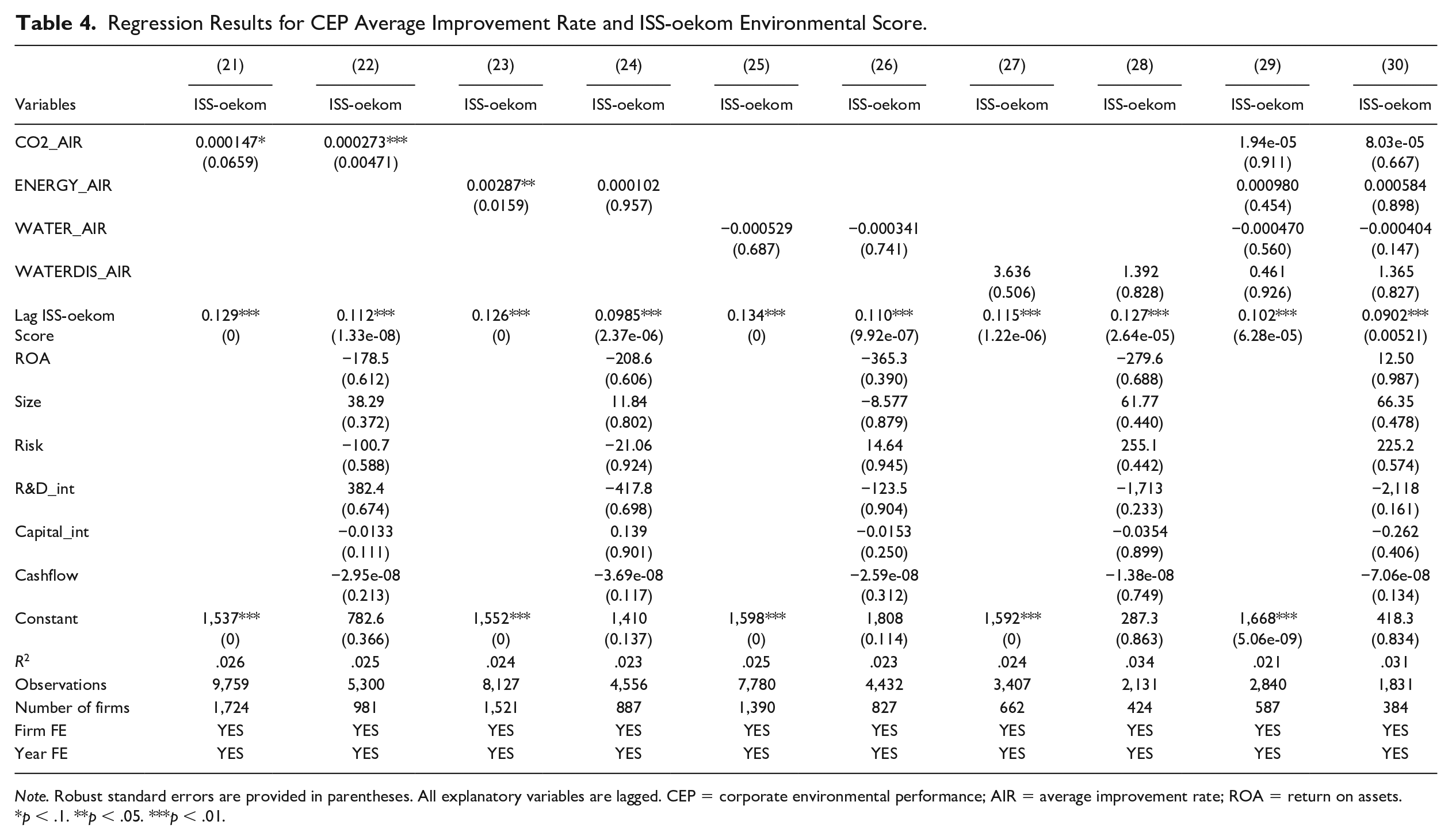
Note. Robust standard errors are provided in parentheses. All explanatory variables are lagged. CEP = corporate environmental performance; AIR = average improvement rate; ROA = return on assets.
p < .1. **p < .05. ***p < .01.
Regression Results for CEP Average Improvement Rate and MSCI ESG IVA Environmental Score.
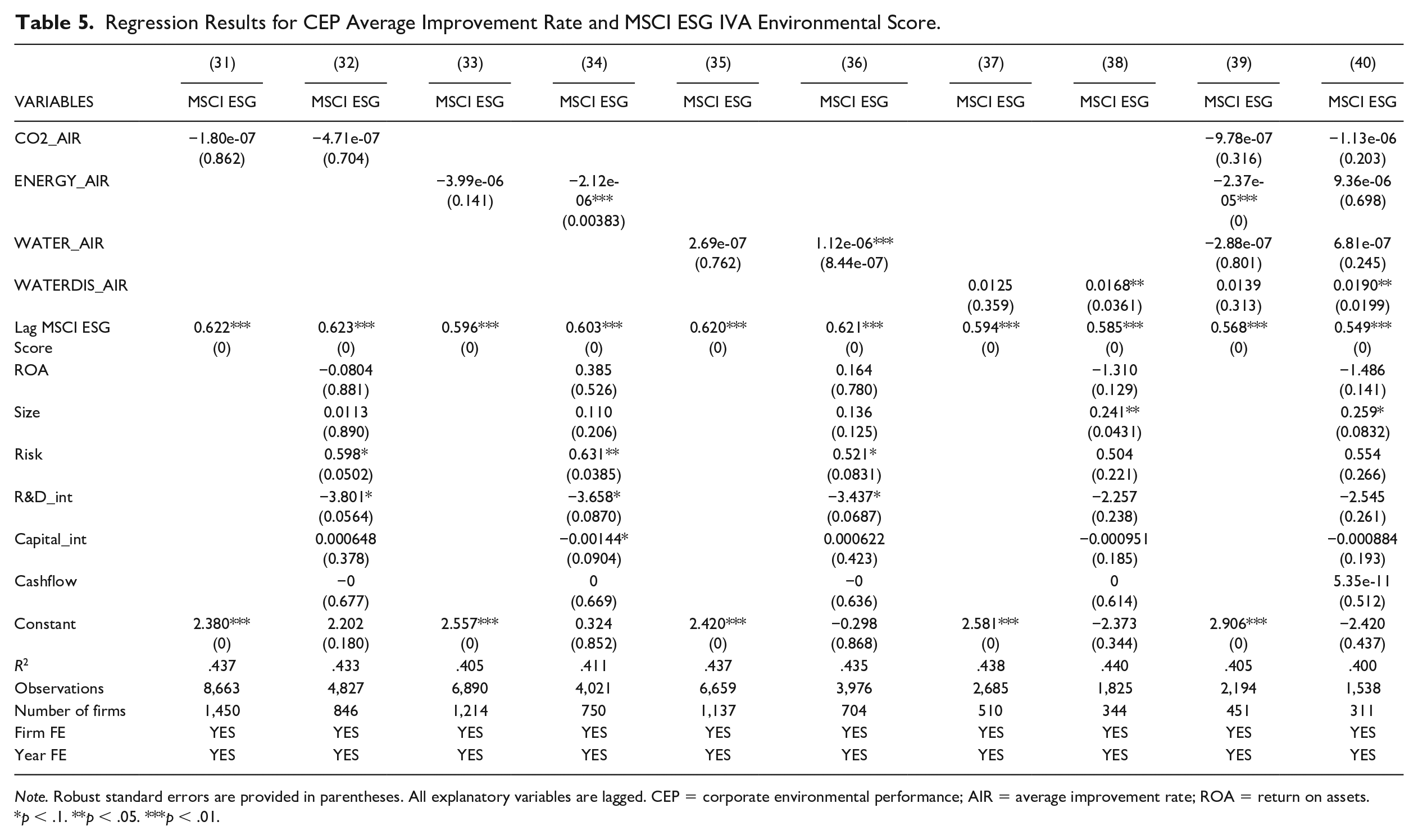
Note. Robust standard errors are provided in parentheses. All explanatory variables are lagged. CEP = corporate environmental performance; AIR = average improvement rate; ROA = return on assets.
p < .1. **p < .05. ***p < .01.
For the vast majority of models in Tables 2 and 3, we cannot find any significant positive relationship between the cumulative improvement effect and aggregated environmental scores. For Model 3 (ΔEnergy_cumulative), we find a significant negative relationship, which is counterintuitive; however, this model is without controls. When controls are included, the significance is removed. As such, no model can confirm the influence of the cumulative improvement effect on environmental scores.
The subsequent two tables (Tables 4 and 5) cover the association between the average improvement rate (AIR) and aggregated environmental scores. For Table 4 covering ISS-oekom, the association between CO2_AIR is both positive and significant with and without the control variables (21 and 22). While it appears that Energy_AIR is also positive and significant (Model 23), it is no longer significant when all controls are included (Table 24). The remaining variables, including Water and WaterDischarge, are not significant. In Table 5, several indicators are significant covering MSCI ESG IVA. Here, Energy_AIR reveals a significant, albeit negative association when including control variables (Model 34). The only positive, significant results between the average improvement rate and MSCI ESG IVA scores are Water_AIR (Model 36) and WaterDischarge_AIR (Model 38). With the exception of these findings, and the one exception found for CO2_AIR and ISS-oekom, the results provide little proof of a significant, positive association between the average improvement rates and aggregated environmental scores.
With the three exceptions mentioned earlier, the results provide little proof of significant, positive associations and mostly reveal insignificant associations between our measurements of continuous CEP improvement and all aggregated environmental scores. The results are contradictory at best, as the combined models in the previously mentioned tables did not produce any significant results. Consequentially, we cannot confirm H1. Thus, continuous CEP improvement—either as cumulative improvement effects or average improvement rates—is not captured in aggregated environmental scores in a meaningful way. In some cases, we obtain the surprising result that corresponding improvements even worsen a firm’s environmental score.
With respect to H2, we provide two tables (Tables 6 and 7) containing 10 models each to test the association between CFP (i.e., ROA and Tobin’s q) and continuous CEP improvement. Table 6 reveals the findings for the cumulative improvement effect and ROA (Models 41–45), followed by the results for the cumulative improvement effect and Tobin’s q (Models 46–50). Similarly, Table 7 represents the association between the average improvement rate and ROA (Models 51–55), as well as the association between the average improvement rate and Tobin’s q (Models 56–60). The tables presenting the four disaggregate measures are presented in the same sequence: CO2, Energy, Water, and WaterDischarge. In addition, we include the four ΔCEP variables one model for testing ROA (Models 45 and 55) as well as Tobin’s q (Models 50 and 60).
Regression Results for CEP Cumulative Improvement Effect and CFP.
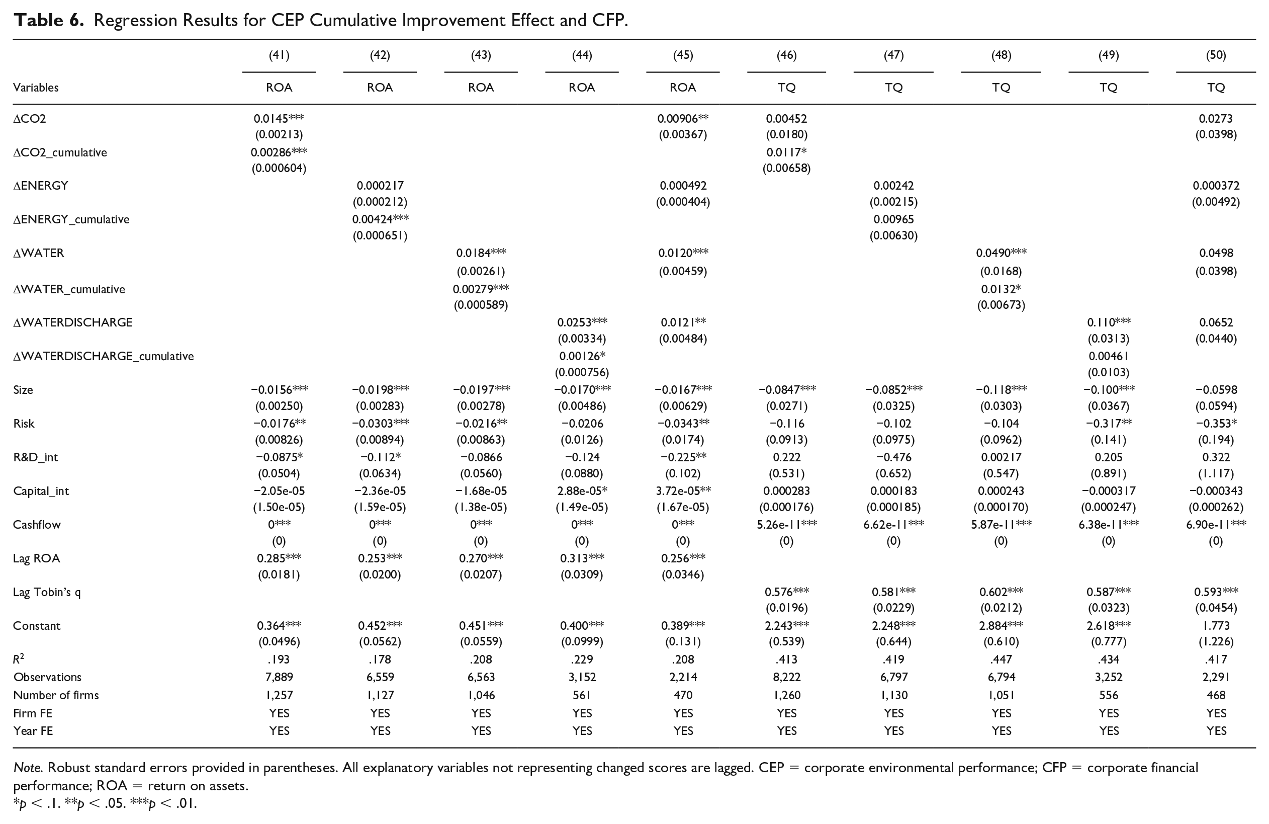
Note. Robust standard errors provided in parentheses. All explanatory variables not representing changed scores are lagged. CEP = corporate environmental performance; CFP = corporate financial performance; ROA = return on assets.
p < .1. **p < .05. ***p < .01.
Regression Results for CEP Average Improvement Rate and CFP.
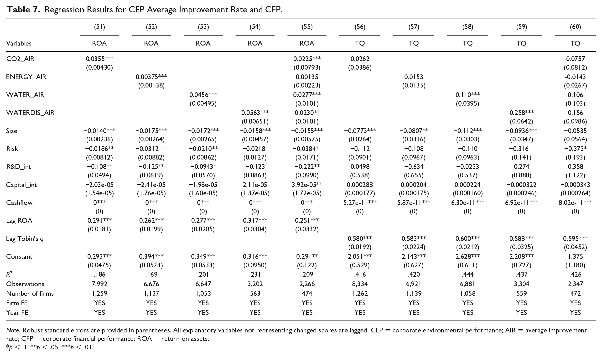
Note. Robust standard errors are provided in parentheses. All explanatory variables not representing changed scores are lagged. CEP = corporate environmental performance; AIR = average improvement rate; CFP = corporate financial performance; ROA = return on assets.
p < .1. **p < .05. ***p < .01.
In total, we regress our independent variables in 20 different panel data models to empirically test H2. For the cumulative improvement effect on ROA (Table 6, models 41 to 45), the first three models are highly significant (at the ρ < 0.01 level); for ΔWATERDISCHARGE_cumulative we obtain significance at the p < .1 level. For Tobin’s q, we obtain significant, positive results for half the models representing the individual effects, including ΔCO2_cumulative (Model 46, b = .0117*, robust SE = 0.00658) as well as ΔWATER_cumulative (Model 48, b = 0.0132*, robust standard error = 0.0231). For several models, however, we did not find significant results, including ΔENERGY_cumlative and ΔWATERDISCHARGE_cumulative. In addition, we also included all ΔCEP variables in one model for ROA and Tobin’s q. For ROA, our results remain quite stable although the variables are partly addressing similar aspects of ΔCEP. In the combined model for ROA (model 45), ΔEnergy_cumulative is not significant. For Tobin’s q, we cannot find any significant results when including all ΔCEP variables in the same model. We speculate that potential overlaps in the variables could cannibalize the individual effects.
For the average improvement rate (Table 7), we obtain very robust results for ROA and only moderate support for Tobin’s q. All models for ROA are highly significant (at the ρ < 0.01 level) with one exception: ENERGY_AIR is not significant in the combined models for ROA (Model 55). For Tobin’s q, two environmental variables are significant, that is, WATER_AIR (Model 58, b = 0.110***, robust standard error = 0.0395) as well as WATERDIS_AIR (Model 59, b = 0.258***, robust standard error = 0.0642); however, both CO2_AIR and ENERGY_AIR are not significant. When all variables are placed in one model for Tobin’s q (Model 60), we cannot see any significant results.
For the second hypothesis, we find mostly positive results. For the accounting-based measure ROA, we find highly significant, positive associations with continuous CEP improvement rates. Even the combined models show mostly significant, positive results. The results for Tobin’s also indicate positive results to a lesser extent. Many individual models reveal a significant, positive relationship with the market-based measure Tobin’s q. Although we did not see any significant results when all variables were placed in one model with Tobins’s q, this may have to do with the combined effects in the models. Thus, the results support H2: continuous CEP improvement—portrayed either as the cumulative improvement effect or as the average improvement rate—is positively associated with accounting-based and market-based CFP indicators.
Robustness Checks
We conduct several robustness checks to test the reliability of our results. KLD scores have been used in many previous studies (e.g., Chatterji et al., 2009; Chen & Delmas, 2011; Eccles et al., 2019; Ortiz-de-Mandojana & Bansal, 2016), and it has been asserted that they are a measure that captures the overall CEP of firms by including both managerial and operational issues (Cheng et al., 2014; Misani & Pogutz, 2015). Accordingly, we are able to obtain firm-level data for more than 200 firms from 2005 to 2012. First, we reassess H1 by analyzing the relationship between CEP improvement and the KLD environmental score (i.e., environmental strengths minus environmental concerns). In addition, we include the individual KLD environmental strengths and KLD environmental concerns for a less biased analysis. For both the cumulative improvement effect and the average improvement rate, we find similar results comparable to our analysis. Thus, this check supported the previous claim that we cannot confirm H1.
Moreover, we also analyzed the consequences of switching from firm-fixed effects to industry-fixed effects and country-fixed effects in all models; however, we cannot find any meaningful differences in the results. While industry-fixed effects detect distinctions within an industry, firm-fixed effects imply that each firm has unique characteristics, and will remove the commonalities on the firm level. Thus, we chose to keep the original models with firm-fixed effects in our paper as these represent a stronger restriction of the model design and account more for firm-specific characteristics.
Finally, we realized that our results could be affected by unbalanced panels. The panel in our models is covering companies from 40 countries and 52 industries focusing on a timeframe from 2005 to 2020. We conducted robustness checks by creating a most balanced panel based on the International Securities Identification Numbers (ISIN). This step significantly reduced the number of firms and observations. The results show that the positive effect of CEP on CFP remains stable in most of the models. The implications of our findings for future research and practice are discussed in the next section.
Discussion and Conclusion
While studies considering the natural resource-based view and proactive environmental strategies have emphasized the importance of continuous improvement as an organizational capability (Hart, 1995; Sharma & Vredenburg, 1998; Surroca et al., 2010), no previous study has empirically investigated the relevance of continuous CEP improvement. Therefore, we present two novel approaches to operationalize continuous CEP improvement: the cumulative improvement effect and the average improvement rate. As such, this study makes a contribution to studies about how organizations can shift toward sustainability via organizational capabilities (e.g., Albertini, 2013; Zollo et al., 2013).
The cumulative improvement effect presents a persistent measure, which considers how many years firms are able to maintain continuous CEP improvement over time. The calculation is based on two components. First, we apply a formula to compute the improvement rate between 2 years, and second, we calculate the accumulative years during which firms have experienced improvements. The concept of a cumulative improvement effect was inspired by previous studies on continuous improvement (Brouwer & van Koppen, 2008; Choi, 1995) as well as by studies dealing with financial signaling (Brouhle & Harrington, 2010; Connelly et al., 2011; Hahn et al., 2015). For example, Brouhle and Harrington (2010) suggest that firms utilize continuous reporting to signal to regulators and investors their environmental responsibility, which is usually based on outcome-based indicators (e.g., CO2 equivalent emissions). Where investors and analysts value proactive disclosure, companies prefer to convey outstanding performance (Clarkson et al., 2008; Hahn et al., 2015). This line of reasoning should hold for continuous CEP improvement as well, especially considering that firms’ environmental performance should constantly improve year on year. A substantiated effect is important for stakeholders, and the cumulative effect is one measure to track progress. Another measure to capture improvement is the average improvement rate, which is adapted from the literature on compound annual growth rate (Chan, 2009). In this article, the average improvement rate represents an amplitude measure, that is, how much improvement can be achieved over the entire time period (2005–2020). It is based on the assumption that the size of continuous improvement should also have a positive association with CFP.
Each approach for measuring continuous CEP improvement tells a different story; one measure is focused on persistence (i.e., time dependent) and the other on amplitude (i.e., size dependent). While the cumulative improvement effect captures the continuity of improvements over a given time frame, it does not reveal the extent or size of the achieved improvement over time. On the contrary, the average improvement rate illustrates the size of the improvement. While the rate is compounded annually, it does not reveal exactly when this improvement was achieved. For example, company A’s emissions could improve significantly in the first year, followed by consecutive years of minor decline. Meanwhile, company B’s emissions might slightly improve every single year over the entire period. The average improvement rate cannot display these differences as the rate of both companies could theoretically be the same. The cumulative improvement effect would make this difference. While each method presents both advantages and disadvantages, neither of our improvement measures is able to cover both persistence and amplitude simultaneously. Thus, it is worth considering both measurements in future research.
This study contributes to the organizations and natural environmental literature in three ways. The first contribution relates to the relevance of continuous improvement as an important organizational capability. Our results empirically demonstrate that continuous CEP improvement has a significant positive association with accounting-based measure (ROA) and with the market-based measure Tobin’s q to a lesser extent. This empirical outcome, based on a large sample over 15 years, confirms previous research that mostly theorized about continuous CEP improvement in the context of operational efficiencies (Hart, 1995; Hart & Milstein, 2003). Given that firms can realize continuous CEP improvement as a capability to increase operational efficiencies by saving resources and preventing waste, they should be able to improve profitability (Ortiz-de-Mandojana & Bansal, 2016). When evaluating the impact of continuous CEP improvement, we can confirm that recurring improvement in terms of reduced energy use and CO2 equivalent emissions will lead to better company profitability; however, this may not (yet) be captured fully in the market value. This finding contests previous findings that empirically show that emission reductions are associated with lower short-term, accounting-based CFP, especially in times of regulatory uncertainty (Delmas et al., 2015; Hart & Ahuja, 1996; King & Lenox, 2002). In contrast, we find a general positive association between CO2 equivalent emissions and CFP for both our measurements of continuous CEP improvement. Two explanations could be that we incorporate a novel way how to measure carbon performance as a continuous improvement and that we incorporate more recent data in our study. However, most importantly, we ascribe this interesting outcome to the fact that we cover the influence of cumulative firm-year observations over time. The other studies neither empirically tested nor controlled for this time effect.
Our study presents interesting results showing continuous improvement in companies’ carbon performance. Continuous CO2 improvements are positively associated with accounting-based CFP (i.e., both improvement rates—ΔCO2_cumulative and CO2_AIR—are significant with ROA); however, the association is only partially captured with market-based CFP (i.e., only ΔCO2_cumulative effect is significant with Tobin’s q). We discover that ongoing CEP improvements capture internal efficiency; yet it appears that the market is either unaware of such improvements or does not price this information. If the former is truly the case, companies should intensify the disclosures of continuous improvements. If the latter is true, further studies should be conducted to establish that our findings hold true in various research contexts. Based on the results, financial markets will increasingly consider continuous CEP improvement as a reflection of good management practices (King & Lenox, 2002; Waddock & Graves, 1997) and, as such, is financially material.
Our second contribution relates to the literature covering the validity and consistency of aggregated scores provided by sustainability rating agencies (Berg et al., 2019; Chatterji et al., 2016; Eccles et al., 2019). We are able to contribute to this literature by demonstrating that continuous CEP improvement is not adequately reflected in aggregated environmental scores provided by sustainability rating agencies, including ISS-oekom, MSCI ESG IVA, and KLD. We find that, with only a few exceptions, the bulk of continual CEP improvements have no meaningful effect on environmental scores. The detected inconsistencies between continuous CEP improvement and aggregated environmental scores are a starting point for further understanding of this relationship and further debate about the consistency of sustainability ratings. One potential reason for our insignificant results when testing H1 may be due to the underlying methodologies, that is, the data construction methods of aggregated environmental scores (Berg et al., 2019). These scores are typically based on multiple environmental criteria, albeit with limited transparency about how the criteria are exactly aggregated and weighted (Escrig-Olmedo et al., 2017), as this is typically the intellectual property of the individual agencies. Berg et al. (2019) acknowledge that these weightings, including the issues covered (i.e., scope) and the manner in which these issues are calculated (i.e., measurement), can explain a huge amount of the divergence between ratings.
Nevertheless, the data providers have claimed that environmental scores incorporate outcome-based operational indicators as well as process-based indicators (Misani & Pogutz, 2015; Trumpp et al., 2015). Process-based indicators deal with environmental management policies, norms, and systems, which are mostly of a rather static nature (i.e., whether a company has an environmental policy or not). When such indicators are aggregated, they may dilute and diminish the relevance of outcome-based operational areas with greater variation, such as CO2 or water emissions. Thus, aggregated environmental scores seem to be inundated by static properties of CEP, which may weaken the more dynamic effects of continuous CEP improvement.
Our third and final contribution considers a more practical point of view, in particular that our results have major implications for sustainability-oriented investors. Such investors often rely on the so-called best-in-class approach (GSIA, 2021). If a best-in-class approach based on aggregated environmental scores was effective from a purely environmental point of view, we would expect improvement to be reflected in these scores. We discover, however, that these scores do not capture superior CEP based on continuous improvement. As such, best-in-class screenings cannot fulfill this purpose—that is, they do not filter out firms that have a bad improvement record. If investors seek to identify companies that in fact improve their CEP outcomes, they should apply a best-in-progress approach. At the same time, this approach also makes sense from a materiality point of view: our results reveal that continuous CEP improvement has a significant, positive association with CFP. Thus, managers, investors, and academics should not rely merely on aggregated environmental scores provided by sustainability rating agencies and best-in-class screenings. Instead, they should consider continuous CEP improvement from a best-in-progress logic to obtain a more holistic picture. In this holistic perspective, a new range of indices could measure and promote firms that improve substantially compared with others in their industry, region, and overall. As a result, investors would strengthen the effort to proactively finance the UN 2030 Agenda for Sustainable Development and the Sustainable Development Goals. This could embrace a larger scope of environmental indicators, including climate mitigation, aspects of biodiversity, and resource efficiency (Howard-Grenville et al., 2017). Companies currently considered environmental laggards could possibly be rewarded for vast environmental improvement. In terms of system-wide improvements, such an effort would be more effective than limiting the investment universe to companies that are already top-rated.
An interesting question is whether there are any distinctions between firms that have consistently improved over extended periods of time and those that have not. For example, are there any significant differences in board composition or R&D activities? These results might explain why we observe these distinctions in continuous CEP improvement. We offer this question for future research. Moreover, while calculating intensities are helpful to focus on efficiency gains by individual firms and to ensure inter-firm comparability, firms could still conceivably maintain the same levels of environmental outputs. A change in the underlying sales figures could explain the resulting change in CEP. Thus, absolute reductions are not achieved. As such, our measurements of continuous improvement do not reveal any information about whether overall contributions to sustainability challenges and goals are achieved—such as a net reduction in CO2 equivalent emissions. Nevertheless, these relative figures still highlight that companies are becoming more eco-efficient. This perspective is important, especially in industries where further growth is desirable from a sustainability point of view. For example, we can expect continued sales growth of wind turbines over the next years. Thus, absolute CO2 equivalent emissions are expected to increase due to the manufacturing of these turbines. At the same time, more efficient manufacturing approaches can lower the relative CO2 equivalent emissions per wind turbine. In addition to the generally positive features of wind turbines for electricity generation, such relative improvements are important steps toward the decarbonization of our economy.
We recognize several limitations of our study. Previous studies have addressed several reliability and consistency issues arising from environmental data taken from third-party providers (Dragomir, 2018; Escrig-Olmedo et al., 2017). According to the data providers, various sources are consulted, including sustainability reports, CDP responses, and questionnaires from rating agencies. We presume that the data source is primarily self-reported by companies. In some cases, independent accounting firms audit these data, but the sustainability rating agencies typically do not disclose this information. As such, we need to trust that this self-reported data has been collected and reported in a correct manner.
As a further limitation of our presented results, we recognize that we do not show the effect of industry association on our dependent variables, especially for environmental scores. While the potential effect that industry has on the environmental score from environmental ratings is contained in the firm-fixed effects, this effect is not transparent in our results. In a separate analysis, however, we ran the models with industry-fixed effects. The results show that no significant deviations occur when comparing industry-fixed effects models to firm-fixed effects models. Another point of discussion is that we did not lag the main explanatory variables in our models by one year behind Tobin’s q. We argued that this might cause a potential misspecification. At the same time, however, given the prevalence of information asymmetry in the provision and availability of a firm’s social and environmental performance (Doh et al., 2010), we cannot rule out the possibility that financial markets may need time to monitor and respond to CEP improvements. We propose that future studies delve into this more as our study does not intend to investigate and explain how and when financial markets react to a specific type of information.
Furthermore, other CEP measurements and indicators exist, which might be equally eligible to act as indicators of continuous CEP improvement. Brouwer and van Koppen (2008) listed multiple indicators in international environmental management frameworks, including the indicators that we selected (e.g., energy use, water use, CO2 equivalent emissions, and water discharge). However, they also provided further physical indicators at the operational level (e.g., total waste) as well as nonphysical indicators pertaining to other managerial aspects (e.g., total environmental investments, amount of environmental education, etc.). While the exclusion of additional physical indicators was due to data restrictions, we purposefully omitted environmental management indicators, as we strongly focus on the operational side of CEP for continuous improvement. Future studies may investigate further CEP measurements and indicators to further generalize our findings. Future research might also broaden the discussion toward the social dimension. For example, social indicators could be applied to cover health and safety issues, working conditions for employees, and labor standards in supply chains. However, the empirical validation of such indicators depends largely on the general availability of data—that is, sufficient observations for many companies over multiple years—as well as the fluidity of data—that is, indicators that can capture change over time.
Footnotes
Declaration of Conflicting Interests
The author(s) declared no potential conflicts of interest with respect to the research, authorship, and/or publication of this article.
Funding
The author(s) received no financial support for the research, authorship, and/or publication of this article.