Sage Journals: Discover world-class research

Abstract

The conditions of sound fields used in research, especially testing and fitting of hearing aids, are usually simplified or reduced to fundamental physical fields, such as the free or the diffuse sound field. The concepts of such ideal conditions are easily introduced in theoretical and experimental investigations and in models for directional microphones, for example. When it comes to real-world application of hearing aids, however, the field conditions are more complex with regard to specific stationary and transient properties in room transfer functions and the corresponding impulse responses and binaural parameters. Sound fields can be categorized in outdoor rural and urban and indoor environments. Furthermore, sound fields in closed spaces of various sizes and shapes and in situations of transport in vehicles, trains, and aircrafts are compared with regard to the binaural signals. In laboratory tests, sources of uncertainties are individual differences in binaural cues and too less controlled sound field conditions. Furthermore, laboratory sound fields do not cover the variety of complex sound environments. Spatial audio formats such as higher-order ambisonics are candidates for sound field references not only in room acoustics and audio engineering but also in audiology.

Keywords

room acoustics spatial sound fields acoustic environment

Introduction

In daily life, human listeners are confronted with sound fields of various kinds. Extreme examples are outdoor sounds in a “free” field and indoor sound in a “diffuse” field. The sound signal of interest for communication, mostly speech, is therefore affected by specific reflection patterns. Furthermore, background noise or other signals must be taken into account. They affect the total perception, impression, intelligibility, interpretation, and segregation into the meaningful acoustic components as well (Bregman, 1990). The total sound signals received and interpreted by human beings carry information not only about the sources such as location and distance, and the semantic content and meaning, but also about the environment. A natural hearing situation is, therefore, composed of many factors not only related to communication as such but also to the surrounding ambience.

When it comes to hearing-impaired patients and hearing aids or cochlear implant technology, the definition of targets for signal processing is crucial. The ideal case for optimum speech intelligibility is surely the complete extraction of reverberation and all competing signals. After the equalization and amplification of the speech component a best match of an anechoic and quiet situation is obtained. All information about the environment is, however, lost. Furthermore, a reasonable social interaction in a group is disturbed since the communication channel is focused in a kind of tunnel to just one communication partner. This might be intentional in some cases, but generally the acoustic environment in its full complexity should be provided to these patients. The spatial cues of sound fields and the complexity of sound fields in various environments are, therefore, of great interest.

Sophisticated signal-processing algorithms exist for hearing devices as well as for communication systems such as hands-free telephone or teleconferencing. These systems are able to handle numerous monaural (in signal domain) and spatial (in spatial domain) effects by internal processing in the communication channel. To optimize the overall auditory quality, however, the exterior sound field, its composition of direct and reflected waves, and its binaural representation are still of interest, since they provide the characteristics of the input signals for the normal hearing system and for the hearing device microphone(s).

The sound field parameters in daily-life environments are revisited for this contribution. The effects on the signals at the individual eardrum or for hearing device microphones are discussed. We have a seemingly good basis for describing the sound-level conditions in laboratory tests of audiological applications (precedence effect, spatial unmasking, for example, cafeteria, etc.), but how do these laboratory sound fields compare with real-world situations? And how can research results in real-world situations be comparable, if we don’t have a clear and robust sound field definition and repeatable sound field reference. After all, the question is, “What do we know about the performance of signal processing (beamforming, echo cancellation, source separation, etc.) in real-world situations?

Sound Fields in Rooms

In a typical communication situation the sound travels along a spherical wave from the source to the listener. At distances larger than 1 m, the wave can even be considered plane because the wavefronts are almost plane and the field impedance at the listener position (without the listener present) is approximately Z₀ = ρc; ρ denotes the density of air and c the speed of sound.

Energy Relations in Classical Room Acoustics

A basic, free, sound field model can thus be composed by assuming a sound incidence of plane waves with a squared sound pressure of

p^{2} = \frac{p_{0}^{2}}{r^{2} / 1 m^{2}}

(1)

(p₀ = sound pressure of the source at 1-m distance). Although the wave fronts are in fact almost plane (see Figure 1), the spherical wave spread in included by accounting for the 1/r² distance law. In level notation and reference to the level in 1-m distance, L₀, this reads

L = L_{0} - 20 \log (r / 1 m)

(2)

Figure 1.

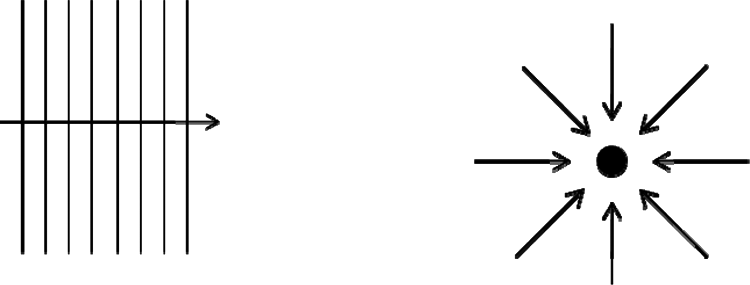
Plane propagating sound waves (left) and diffuse sound field (right)

This basic model is often used to describe the sound field composed by the contribution from a primary talker, mostly frontal incidence. Other talkers, as used in the typical “cocktail party” situation (Blauert, 1996), are placed around the listener at other angles of incidence. The total field is then obtained by summing the plane waves energetically because of incoherent superposition of different broadband sources. The result is often assumed as “diffuse” (see Figure 1).

The imagination of a diffuse sound field is also a useful model to describe sound fields in rooms. At first, no other sources are involved. In this case, the summation concerns delayed and spatially mixed reflected versions of the original source signal. Due to a limited coherence length (transient behavior), the signals must be added energetically as well.

In fields created by more than one source, the signal-to-noise ratio defines the level difference between the one source signal and the competing background signals, p_i, with each of them referred to in 1 m distance, and thus

L_{noise} = 10 \log (\sum_{i} \frac{p_{i}^{2}}{r_{i}^{2} / 1 m^{2}})

(3)

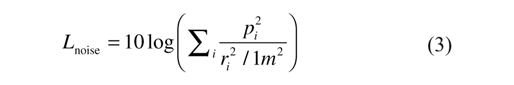
and

\frac{s}{n} [d B] = L - L_{noise} + 10 \log Γ

(4)

10 log Γ denotes the directional characteristics of beamforming or other directional behavior of the listener.

In rooms at distances larger than the reverberation distance, r_c, the same is expressed by the signal-to-diffuse ratio,

\frac{s}{d} [d B] = L - L_{diffuse} + 10 \log Γ

(5)

with

L_{diffuse} = L_{0} - 20 \log (r_{c} / 1 m)

(6)

and

r_{c} = 0.057 \sqrt{\frac{V}{T}} m

(7)

in a room of volume V in m³ and reverberation time T in s. This could be extended by including other sources that excite a diffuse noise field. All in all, a situation where the listener, the talker, and noise sources are in a room yields a level balance that accounts for the signal energies but not for wave superposition of the signals and room response. Ideally, these equations can be applied with power-density spectra in form of band-filtered data.

As mentioned previously, the diffuse sound field is an imagination and academic model assumption (Kuttruff, 2009). In daily-life environments nondiffuse sound fields occur, particularly in noncompact room shapes, coupled rooms, long and flat rooms, and modern architecture with staggered rooms. In case of locally concentrated absorption or reflecting objects in proximity of the listener no diffuse sound field can be expected. The basic equations listed previously do not hold for these examples.

Furthermore, in small rooms with high Schroeder frequency (Schroeder & Kuttruff, 1962) the modal response has to be taken into account. The total room response is given by the stationary room transfer function between the excitation point and the receiver point.

As illustrated in Figure 2, the room response for excitation with stationary signals consists of modes (eigen functions) that are the basic solution of the harmonic wave equation (Helmholtz equation). These modes are also called room resonances. The width and height of the resonance peaks depend on the amount of damping that is typically caused by surface absorption on floor, ceiling, and walls. It can be shown that modes exist in any room and that their density on the frequency axis increases with the square of the frequency. Now it is only a question of basic room parameters such as volume and damping at which frequency neighbored modes overlap. Thus, this frequency response consists of two parts, lower and higher frequencies, separated by the Schroeder frequency

f_{s} = 2000 \sqrt{V / T} H z

(8)

that indeed just depends on the room volume and the amount of damping expressed by the reverberation time. The mostly used definition for f_s is based on the criterion that three modes coincide in the average half-width. It is also important to notice that the transfer function in the region above the Schroeder frequency is extremely complicated and apparently stochastic. The curve in the high-frequency region in Figure 2 depicts an average level and an average spacing of maxima and minima that can as well be predicted from the room volume and the reverberation time. But other design factors such as room shape and distribution of absorption cannot be identified at all.

Figure 2.

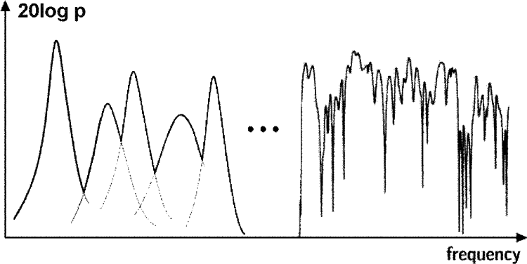
Stationary room transfer function of the rms sound pressure, p, at an arbitrary receiver point

The range of Schroeder frequencies in real-world environments is about 800 Hz in car compartments and below 20 Hz in large rooms. The discrepancy in the definition of the “frequency range of interest” (particularly for speech) with reference to the Schroeder frequency is obvious. It may be far above or below the Schroeder frequency. None of the modal or stochastic behavior can be assumed to be valid throughout the frequency range of interest. We will now focus on the physical behavior of such modal room sound fields.

Wave Acoustics and Fine Structure of Room Transfer Functions

In the statistical domain of the room transfer function the fine structure is stochastic. Even small changes in temperature, humidity, or air movement due to air condition cause large changes in fine structure, particularly in the phase response. The exact physical solution of the statistical mode domain is thus instable and not appropriate for practical application. Apart from that, the listening experience in rooms is not sensitive to those small changes in the environmental conditions. For discussion of the room acoustic perception, the signal and its spectrum and transient behavior comes into play. Purely harmonic signals, as used in the solution of the stationary room transfer function, are hardly relevant in daily life. Speech and noise are broad-band and transient signals. Therefore, luckily, the fine structure is not crucial as it seems at first sight. But the transient response, given the fine structure of the room impulse response, is crucial for the room acoustic perception.

The specification of sound fields in time domain can easily be defined by series of reflections (see Figure 3).

h_{j} (t) = \sum_{j = 1}^{N} p_{j} \cdot δ (t - t_{j})

(9)

Figure 3.

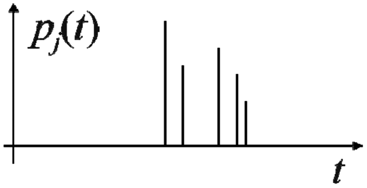
Impulse response

By carrying out a Fourier transformation we obtain the corresponding result in the frequency domain. It consists of overlapping comb filters.

H_{j} (f) = \sum_{j = 1}^{N} p_{j} \cdot e^{- i 2 π ftj}

(10)

This fact is illustrated in Figure 4 by following a listener during a day along his or her situation in various environments: a sidewalk along a street, a passenger compartment of a car, a church, and a classroom (examples). The car has a volume of 2.7 m³ and a Schroeder frequency of 350 Hz, the church has 160,000 m³ and a Schroeder frequency of 10 Hz, and the classroom 300 m³ and 80 Hz, respectively. The sound field conditions are discussed by using the magnitude spectra of sound transmission from a talker to the listener.

Figure 4.

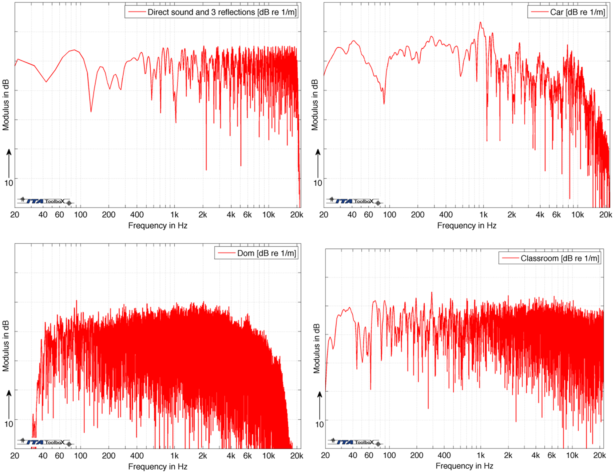
Typical transfer functions (magnitude) of four acoustic environments: sidewalk (upper left), car compartment (upper right), church (lower left), classroom (lower right)

To discuss the specific effects of those transfer functions, we must keep in mind that speech communication signals are transient signals. The fine structure of the transfer functions will not be effective in detail. Nevertheless, it is obvious that the environments affect the speech spectrum significantly and specifically. This fact is even more pronounced if spatial attributes are added. After all, every room response has a specific spatial/temporal or spatial/spectral character that is not taken into account by the simple global-level Equations 1 to 6.

To better account for the specific room acoustic environment, at least the direct and reverberant field should be classified with regard to the signal and background noise components. This is discussed in the next section.

Room Classification by Coherence Estimation

State-of-the-art room classification suffers from the problem that the results depend on the signal used or evaluated. This is because reverberation can be present already in the signal (imagine music from TV or home audio from a hall recording), or reverberation can be introduced by the actual listening environment. Recently, Scharrer and Vorländer (2010) invented a novel room classification technique that is independent of the signal. Thus, any kind of signal can be processed to estimate the room volume, the reverberation time, and the signal-to-noise ratio, provided the room sound is evaluated at two positions in the room. The method takes benefit from the specific complex room transfer functions. Two sensors are required (e.g., binaural microphones or bilateral hearing aid microphones). The estimation is then calculated from the discrete coherence function between the two channels. The crucial point is that this coherence estimate depends on the block length of the discrete processing implementation.

Figure 5.

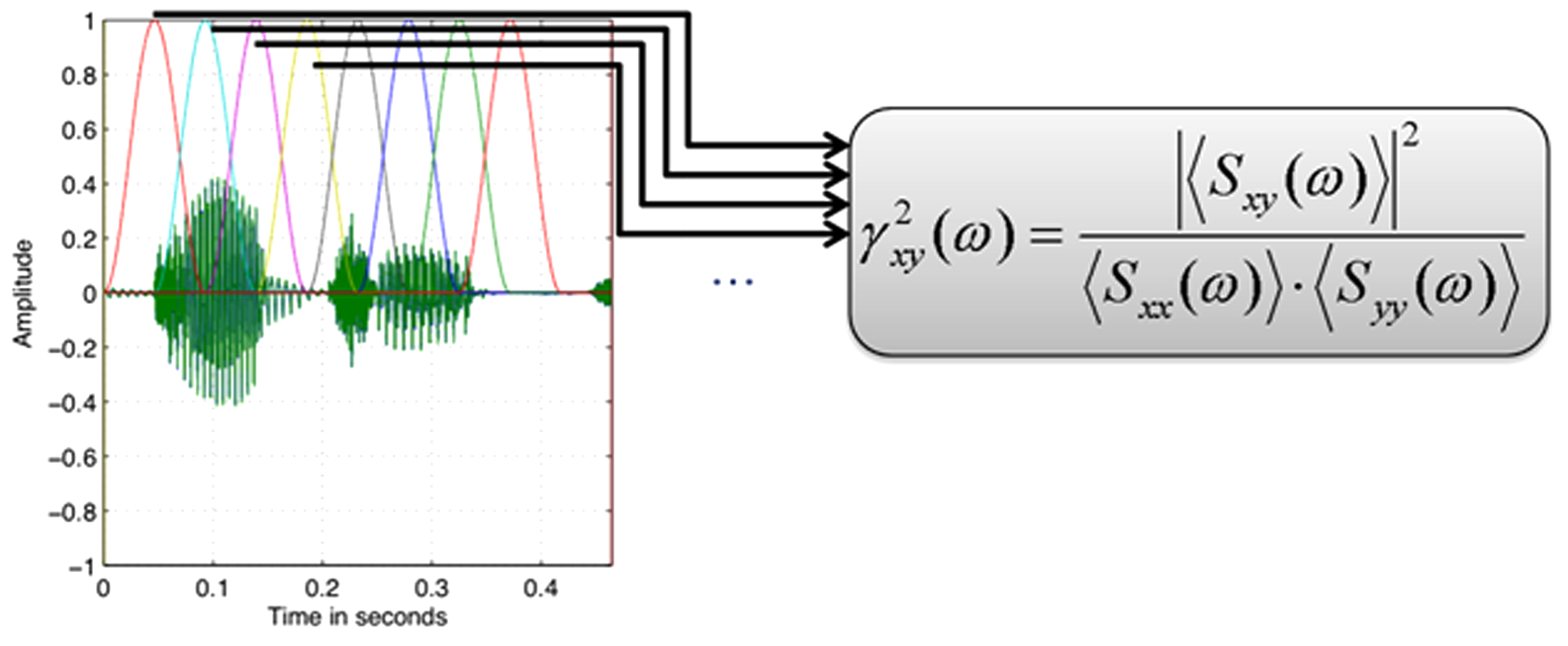
Blockwise estimation of binaural coherence, (Scharrer & Vorländer, 2010)

The result, the coherence estimate versus block length function, CEF, shows specific features depending on room volume, reverberation time, and signal-to-noise ratio.

Figure 6.

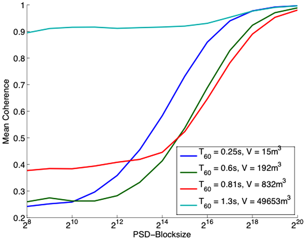
Dependence of the spatial coherence estimate, CEF, on room acoustics (Scharrer & Vorländer, 2010)

Although the evaluation is computationally too heavy to be implemented in hearing aids, it is promising and is worth being investigated. If the conditions of the acoustic environment can be estimated, settings of signal processing parameters for beamforming, echo cancellation, and other techniques can be optimized.

Spatial Attributes in Room Acoustics

Spatial attributes in room acoustics have been analyzed since the 1970s. It was found that in concert-hall acoustics a certain amount of lateral reflections is required. Early lateral reflections create a sufficient apparent source width, and late lateral sound creates an impression of listener envelopment (Barron, 1971). The objective measures for describing lateral reflections are using directional microphones or binaural impulse responses and cross-correlation quantities such as IACC (Ando, 1977). With the IACC a reference is made to a certain dummy head, which must be standardized in shape and size to represent a good match with the heads of an average human population (see section “Individual Cues in Binaural Technology”).

Independently of research on room acoustic perception, physical properties of room sound fields have been studied until today to record and reproduce spatial sound (Abhayapala & Ward, 2002; Fazi, Nelson, Christensen & Seo, 2008; Zotter, 2009). The latter is obviously connected with the recording task in audio engineering and corresponding standardization of spatial audio formats. A very promising technique of spatial audio is the decomposition into spherical harmonics (SH). This technique is similar to a Fourier transformation. It involves an orthogonal function basis, the spherical harmonics. The spherical harmonics are elementary source directivity functions such as monopole, dipole, quadrupole, and so on. They can be combined in linear superposition to describe the arbitrary distribution of directivities in spatial angles (Gerzon, 1976). The maximum order of such harmonics just depends on the spatial fine structure of the directional characteristic. It is clear that this concept can be applied not only for source and listener directivities but also for decomposition of spatial sound fields incident on the listener (Balmages & Rafaely, 2007; Ahrens & Spors, 2009). The SH technique in recording and reproduction is known as Ambisonics or HOA (higher-order Ambisonics; Poletti, 2005). The crucial question is, which spatial format or measurement technique can serve as a general descriptor of three-dimensional sound fields in real life (see “Reference to a Spatial Interface—A Solution for the Future?”).

Spatial aspects of Speech Intelligibility in Complex Sound Fields

One of the often-cited examples in communication situations is the conversation at a cocktail party. The so-called cocktail party effect is a well-known example for selective attention. In this situation, the relevant information is masked by irrelevant speech, noise, and reverberation. This phenomenon is, therefore, subject to research in audiology and cognitive psychology. In classical studies, sounds are presented to the test participants via headphones or loudspeakers in very simple arrangements. A spatially distributed scene is often just approximated by dichotic headphone presentation or by a setup of few loudspeakers around the listener. From the physical point of view, the spatial listening environment is well studied but is only studied within laboratory conditions; thus, results derived from a laboratory-based study cannot be considered as a sufficient interpretation of real-life source distributions. Needless to say that all neurophysiological models of binaural hearing, source segregation, and semantic interpretation are related to those simple sound field conditions as well. This fact might be the reason why we still have to do with unsatisfactory models of neurological signal processing, speech recognition in noisy environments, and appropriate signal-processing algorithms for signal-to-noise improvements implemented in hearing aids. It is known, for example, that the binaural masking-level difference, BMLD, is a significant feature of source segregation and speech enhancement, in case the speech and the noise are spatially distributed (Colburn & Durlach, 1978).

To define a robust spatial sound field reference, the crucial question is exactly the same as mentioned previously in the disciplines of room acoustics and audio engineering: Which spatial format or measurement technique can serve as a general descriptor of three-dimensional sound fields in real life?

The first attempts to create a reference focused on binaural technology. In binaural representation of eardrum signals, the spatial attributes are included properly, at least theoretically. The aim behind the standardization of KEMAR; International Electrotechnical Commission [IEC] 60959, 1990) was to achieve a good reproducibility for measuring hearing aids. Later, in the International Telecommunication Union, other dummy heads were standardized, or more precisely, more dummy heads shapes were allowed in a larger tolerance range to harmonize the variety of binaural measuring devices (International Telecommunication Union [ITU], p.58, 1993).

Individual Cues in Binaural Technology

The latest findings in binaural recording technology is based on measurements of head-related transfer functions, HRTF, on a population in the U.S. Army in the 1960s (Burkhard & Sachs, 1975) and on ear canal impedances (Shaw & Teranishi, 1968). It was first applied to measure hearing aids under in situ conditions. Furthermore, it became the de facto standard for virtual acoustics and home video systems (Mannerheim & Nelson, 2005). In the 1980s, Genuit (1984) developed the technology of artificial heads with regard to specific geometric features of human heads. He introduced a parametric model and a robust structural averaging procedure to calculate the diffraction field at the head. All these dummy heads were tested in intercomparisons of HRTF, headphone transfer functions, and hearing protectors. Hearing aids are in the focus, including all kinds of telephones.

The model-based dummy heads may serve as a good reference. If, however, spatial sound fields are to be used in listening tests, problems occur, and these are caused by a mismatch of the individual head parameters of the test participant with the rather simplified dummy-head data. Replicas of actual persons still yield significantly better results than the standardized dummy heads (Minnaar, Olesen, Christensen, & Møller, 2001; Møller, Sørensen, Hammershøi, & Jensen, 1995; Schmitz, 1995). It is also interesting that those replicas are bigger in the head size than KEMAR and the other standard heads. This is, again, led to some research on the relevance of head dimensions and determination of the best average (Vorländer & Fels, 2008).

It can be also shown that individual binaural cues play an important role when it comes to children. Fels et al. (Fels, Buthmann, & Vorländer, 2004) investigated the differences between head dimensions of adults and children and the differences between individual cues of the ear canal (Fels, 2007). The most significant result is that children are not scaled adults. As for the whole body, the head dimensions have specific features that cannot be achieved by simply scaling the frequency range for smaller sizes.

Figure 7.

Head models of infant, child and adult and head-related transfer functions in the horizontal plane (top) and in the median plane (bottom), (Fels, Buthmann, & Vorländer, 2004)

Uncertainties, therefore, have to be faced when listeners are placed in a binaural listening scenario. These differences are caused by individual binaural cues.

Positioning Uncertainties in Laboratory Tests

Not only the individual binaural cues may cause uncertainties, but, in laboratory tests, a very simple error can occur that is caused by a lack of precision of head positions in listening tests. Let us consider once again the typical scenario of a test of BMLD in the laboratory or in a real sound field of high complexity. Consider that the researcher or test operator describes the test conditions by giving information about the listening room, the loudspeaker placement in direction and distance. And possibly a table is used for filling out a questionnaire, see Figure 8. This is not even a very complex sound field, but a situation from daily life in a classroom or a cafeteria. Accordingly, this situation is often used to simulate those environments.

Figure 8.

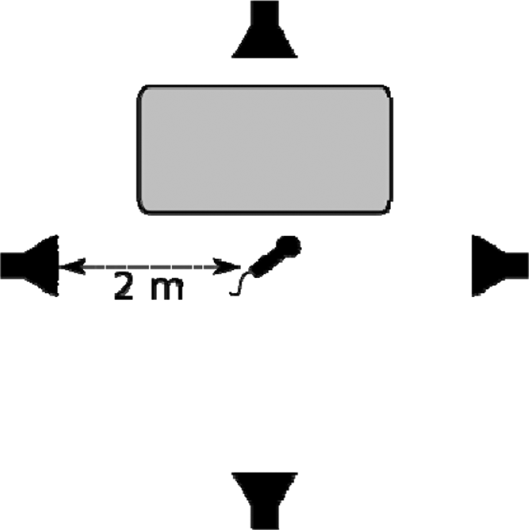
Example of a test scenario for a test participant sitting at a table. The speech signal is presented from the front and the noise additionally from surround loudspeakers. The microphone marks the reference position of the test participant at the height of the ears

We now imagine that the setup is calibrated with a microphone at the reference position, and speech and noise levels are adjusted accordingly. Then the test participants are asked to sit down at the table. In such experiments, however, it is hardly checked whether the head positions of the individual test participants are located exactly at the reference point. Some persons are taller than others. And some persons may move the head to the side or turn the head slightly for getting benefit from dynamic binaural cues.

In the following, the real speech and noise levels and the SNR in a region around the reference point are calculated and compared with the nominal (calibration) SNR levels at the reference point. It is illustrated that the indication of SNR suffers from uncertainties caused by apparently small deviations of the head position from the calibration position. Figure 9 shows the level differences in the sound field spectra between a calibration measurement of the signal levels and noise levels at the reference head position, compared to an actual listening position only 20 cm apart from the reference position. At increasing SNR, the effect becomes more prominent that is caused by the influence of the dominating speech signal interfering with its reflection at the table. A distance mismatch of 20 cm happens easily due to movement of the test participant’s chair or due to differences in the head positions with reference to the table. If the calibration condition is not defined properly or if the test condition is not appropriately matched in height of the test participant’s seat, we obtain results with a level uncertainty illustrated in Figure 9. This uncertainty will be inherent in the test results, possibly in tests during development of hearing aid signal processing and finally in fitting.

Figure 9.

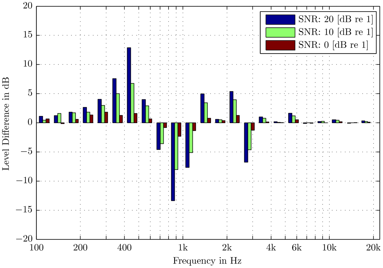
Sound-pressure-level uncertainties in one-third octave bands. Differences between the actual sound level at the listening position compared to the level at the reference position. The distance between the listening position and the reference position is 20 cm (in height)

Thus, given the variance in the physical size of the test participants—participants can be short or tall—the concept of using a reference sound field of one speech source and surround “diffuse” noise sources may create uncertainties of more than 10 dB, and these uncertainties depend on the signal-to-noise ratio.

Reference to a Spatial Interface—a Solution for the Future?

The reasons mentioned previously may cause that the specific input signals into the auditory system are only roughly identified and that unknown amplitude and phase cues often prohibit comparability. Even if the setup was described in detail, the degree of complexity would still be low if we compare this with real sound fields in rooms, with early distinct and late diffuse reflection patterns. The question is how to achieve a sufficient sound field reference instead of using apparently insufficient reference sound fields. The solution is not ready yet, but a promising way of sound field reference data is using spatial data formats that form an intermediate step from the spatial sound field to binaural signals. If the directional sound field is known, its transformation into binaural signals can be done subsequently and individually (Meyer, & Elko, 2002) (Noisternig, Sontacchi, Musil, & Höldrich, 2003) (Song, Ellermeier, & Hald, 2008). The spatial sound field is, thus, a basis for postprocessing in various applications in general. A digital signal format in three-dimensional space is required for documentation of test scenarios with temporal, spectral, and spatial attributes. This format could be higher-order ambisonics, HOA, as discussed earlier. To reach the goal of a robust sound field reference, cooperation is required among groups of researchers from different fields such as room acoustics, audio engineering, and audiology.

Conclusions

Listening conditions for hearing aid development and fitting require a certain degree of significance concerning the environment. The typical reference sound fields such as free field and diffuse fields, however, do not exist in the real world. What is needed is a sound field reference rather than a set of reference sound fields.

Candidates for sound field references are descriptors for room classification, better representations of individual binaural signals, and spatial audio formats. But the first two options are not ideal due to lack of completeness of the information and of general applicability. The latter technique, spatial audio technology, is well known in audio engineering and music recording, but not yet in room acoustics and hearing aid technology. It is suggested to enhance cooperation among the respective scientific communities in order to stimulate further progress in development of robust sound field descriptors for complex environments.

Footnotes

This work was presented at IHCON 2010, Lake Tahoe, August 11-15, 2010.

The author declared no potential conflicts of interests with respect to the authorship and/or publication of this article.

The author received no financial support for the research and/or authorship of this article.

References

Abhayapala

T. D.

Ward

D. B.

(2002). Theory and design of high order sound field microphones using spherical microphone array. Proceedings ICASSP 2002, 2, 1949-1952.

Ahrens

Spors

(2009). Spatial encoding and decoding of focused virtual sound sources. Ambisonics Symposium, Graz, Austria.

Ando

(1977). Subjective preference in relation to objective parameters of music sound fields with a single echo. Journal of the Acoustical Society of America, 62, 1436-1441.

Balmages

Rafaely

(2007). Open-sphere designs for spherical microphone arrays. IEEE Transactions on Audio, Speech and Language Processing, 15(2), 727–732.

Barron

(1971). The subjective effects of first reflections in concert halls—the need for lateral reflections. Journal of Sound and Vibration, 15, 475-494.

Blauert

(1996). Spatial hearing: The psychophysics of human sound localization. Cambridge: MIT Press.

Bregman

A. S.

(1990). Auditory scene analysis: The perceptual organization of sound. Cambridge: MIT Press.

Burkhard

M. D.

Sachs

R. M.

(1975). Anthropometric manikin for acoustic research. Journal of the Acoustical Society of America, 58, 214-222.

Colburn

Durlach

N. I.

(1978). Models of binaural interaction. In Carterette

E. C.

Friedman

M. P.

(Eds.), Handbook of perception (pp. 467-518). San Diego, CA: Academic Press.

10.

Fazi

F. M.

Nelson

P. A.

Christensen

J. E. N.

Seo

(2008). Surround system based on three dimensional sound field reconstruction. 125th AES Convention, San Francisco.

11.

Fels

(2007, December 6-8). Ear canal impedances of children and adults—investigations with simulation and measurements. Proceedings of the 4th International Pediatric Conference: Sound Foundation Through Early Amplification, Chicago.

12.

Fels

Buthmann

Vorländer

(2004). Head-related transfer functions of children. Acta Acustica United With Acustica, 90, 918-927.

13.

Genuit

(1984). Ein Modell zur Beschreibung von Außenohrübertragungseigenschaften (A Model for the description of the transfer function of the external ear). PhD Dissertation, RWTH Aachen University, Aachen, Germany.

14.

Gerzon

M. A.

(1976). Multidirectional sound reproduction systems (UK Patent No. 3 997 725).

15.

International Electrotechnical Commission. (1990). Provisional head and torso simulator for acoustic measurements on air conduction hearing aids (IEC 60959; adopted into IEC 60318-7). Geneva, Switzerland.

16.

International Telecommunication Union. (1993). Head and torso simulator for telephonometry (ITU P. 58). Geneva, Switzerland.

17.

Kuttruff

(2009). Room acoustics. 5th edition, Taylor & Francis, New York.

18.

Mannerheim

Nelson

P. A.

(2005). Adaptive loudspeaker based virtual acoustics imaging system (Technical Report No. 05/07). Southampton, UK: Institute of Sound and Vibration Research.

19.

Meyer

Elko

G. W.

(2002). A highly scalable spherical microphone array based on an orthonormal decomposition of the soundfield. Proceedings ICASSP, 1781-1784.

20.

Minnaar

Olesen

S. K.

Christensen

Møller

(2001). Localization with binaural recordings from human and artificial heads. Journal of the Audio Engineering Society, 49, 323-336

21.

Møller

Sørensen

M. F.

Hammershøi

Jensen

S. B.

(1995). Head-related transfer functions of human subjects. Journal of the Audio Engineering Society, 43, 300-321.

22.

Noisternig

Sontacchi

Musil

Höldrich

(2003). A 3D ambisonic based binaural sound reproduction system. 24th International Conference on Multichannel Audio, Banff, Alberta, Canada.

23.

Poletti

M. A.

(2005). Three-dimensional surround sound systems based on spherical harmonics. Journal of the Audio Engineering Society, 53(11), 1004-1025.

24.

Scharrer

Vorländer

(August, 2010). Blind reverberation time estimation. Proceedings of the International Conference on Acoustics, Sydney, Australia.

25.

Schmitz

(1995). Ein neues digitales Kunstkopfmesssystem (A new digital dummy head measurement system). Acustica, 81, 416-420.

26.

Schroeder

M. R.

Kuttruff

K. H.

(1962). On frequency response curves in rooms. Comparison of experimental, theoretical and Monte Carlo results for the average frequency spacing between maxima. Journal of the Acoustical Society of America, 34, 76-80.

27.

Shaw

E. A. G.

Teranishi

(1968). Sound pressure generated in an external-ear replica and real human ears, by a nearby point source. Journal of the Acoustical Society of America, 44, 240-256.

28.

Song

Ellermeier

Hald

(2008). Using beamforming and binaural synthesis for the psychoacoustical evaluation of target sources in noise. Journal of the Acoustical Society of America, 123(2), 910-924.

29.

Vorländer

Fels

(2008). The next generation of artificial heads. Proceedings of the 2nd Joint Meeting ASA-EAA, Paris.

30.

Zotter

(2009). Analysis and synthesis of sound-radiation with spherical arrays. Doctoral thesis, University of Music and Performing Arts Graz, Austria.

Sound Fields in Complex Listening Environments

Abstract

Keywords

Introduction

Sound Fields in Rooms

Energy Relations in Classical Room Acoustics

Wave Acoustics and Fine Structure of Room Transfer Functions

Room Classification by Coherence Estimation

Spatial Attributes in Room Acoustics

Spatial aspects of Speech Intelligibility in Complex Sound Fields

Individual Cues in Binaural Technology

Positioning Uncertainties in Laboratory Tests

Reference to a Spatial Interface—a Solution for the Future?

Conclusions

Footnotes

References