We investigate a scalar partial differential equation model for the formation of biological transportation networks. Starting from a discrete graph-based formulation on equilateral triangulations, we rigorously derive the corresponding continuum energy functional as the Γ-limit under network refinement and establish the existence of global minimizers. The model possesses a gradient-flow structure whose steady states coincide with solutions of the p-Laplacian equation. Building on this connection, we implement finite element discretizations and propose a novel dynamical relaxation scheme that achieves optimal convergence rates in manufactured tests and exhibits mesh-independent performance, with the number of time steps, nonlinear iterations, and linear solves remaining stable under uniform mesh refinement. Numerical experiments confirm both the ability of the scalar model to reproduce biologically relevant network patterns and its effectiveness as a computationally efficient relaxation strategy for solving p-Laplacian equations for large exponents p.
In this paper, we study the scalar partial differential equation system modeling the formation of biological transportation networks,
for the scalar pressure field of the fluid transported within the network and the scalar conductance (permeability) , with metabolic constant and metabolic exponent . We assume the validity of Darcy’s law for slow flow in porous media, connecting the flux q of the fluid with the gradient of its pressure via the action of the permeability ,
The total permeability is assumed to be of the form , where the scalar function describes the isotropic background permeability of the medium. The source term in the mass conservation equation (1) is to be supplemented as an input datum and is assumed to be independent of time. We pose (1), (2) on a bounded domain , , with smooth boundary .
For (1), we prescribe the homogeneous Neumann boundary condition
where is the outer normal vector to the boundary . We note that (2) is a system of ordinary differential equations (ODEs) (coupled through the term ) and, therefore, no boundary condition can be prescribed for .
We prescribe the initial condition
with almost everywhere in Ω.
A fundamental structural property of the systems (1)–(2) is that it represents the constrained -gradient flow associated with the energy functional
where is a solution of the Poisson equation (1) subject to homogeneous Neumann boundary condition (3). We note that this property only holds when the source term does not depend on time. The first term in (5) describes the kinetic (pumping) energy necessary for transporting the medium, while the second term is the metabolic expenditure of the network. It is well known that for , the energy functional is convex, see [1,2]. Based on this fact, we construct a unique solution of (1)–(2) as the corresponding gradient flow. We refer to [3,4] for further details.
A variant of the systems (1)–(2) was proposed and studied in Hu and Cai [5,6], where the local permeability of the porous medium is described in terms of a vector field. Detailed mathematical analysis was carried out in a series of papers [3,7–9] and in [10–12], while its various other aspects were studied in [2,13–16]. Another variant with a diagonal permeability tensor was derived formally in Haskovec et al. [17] from the discrete network formation model [16]. The corresponding continuum energy functional was obtained as a limit of a sequence of discrete problems under refinement of the network, with geometry restricted to rectangular networks in two dimensions. In Haskovec et al. [14], the process was carried out rigorously, in terms of the Γ-limit of a sequence of discrete energy functionals with respect to the strong -topology. In Haskovec et al. [1], this was generalized to general symmetric, positive semi-definite conductivity tensors. The continuum energy functional was obtained as a refinement limit of discrete problems on a sequence of triangular meshes. However, the derivation was only formal. Finally, in Alves and Haskovec [18], a graphon limit has been derived rigorously, where (1) is replaced by an integral equation.
Let us note that as long as we are interested in calculating the minimizers of the energy functional (5), i.e., the steady states of the systems (1)–(2), for metabolic exponents , it is sufficient to work with the scalar conductivity c. Indeed, setting and for simplicity, the steady-state condition for (2) reads . Inserting into (1) gives the p-Laplacian equation
Note that the exponent for and when . Now, the steady-state condition for the model [1] with tensor-valued conductivity reads . Therefore, C is the rank-one tensor , and the flux reads
Inserting into the Poisson equation then gives (6). Consequently, the equilibrium fluxes of both the tensor- and scalar-valued models coincide and are given by , where u solves (6). We conclude that it is sufficient to work with the scalar-valued conductivity.
Among the most successful numerical solvers for the p-Laplacian are preconditioned gradient descent algorithms [19], barrier methods [20], and quasi-Newton methods [21]. Within this landscape, relaxed Kačanov iterations [22,23] can be considered the gold standard, as they combine robustness with provable convergence. Semi-implicit formulations arising from gradient flows associated with the p-Laplacian energy have also been investigated [24]. In contrast, the gradient flow proposed here serves as a dynamical relaxation: time integration regularizes the nonlinearity and drives the solution to the p-Laplacian steady state, offering an alternative to classical stationary iterations and complementing existing relaxation techniques.
Numerical experiments validate our approach as a competitive alternative to existing relaxation techniques, confirming optimal convergence rates for manufactured solutions and demonstrating robustness for large values of p without the need for adaptive mesh refinement. Numerical evidence indicates that the algorithm can also be applied in the presence of mixed, non-homogeneous Dirichlet and Neumann boundary conditions for (1), and that it exhibits mesh-independent convergence, in the sense that the number of required time steps, nonlinear iterations, and inner linear solver steps remains essentially unaffected by mesh resolution.
This paper is structured as follows. In Section 2, we rigorously derive the energy functional (5) with from the discrete model [5,6] in the refinement Γ-limit of a sequence of triangulations. We also construct its global minimizers in the class of uniformly Lipschitz continuous functions as limits of minimizers of the discrete problem. In Section 3, we consider the numerical approximation of the systems (1)–(2) with general boundary conditions. First, in Section 3.1, we consider the case and demonstrate its ability to generate two-dimensional network patterns. Then, in Section 3.2, we solve (1)–(2) with until equilibrium to obtain solutions of the p-Laplacian equation (6).
2. Derivation from the discrete model in two dimensions
The goal of this section is to provide a derivation of the continuum energy functional (5) with as a limit of discrete energy functionals [5,6] posed on a sequence of equilateral triangulations of a bounded polygonal domain . Without loss of generality, we will assume that is a constant. For the sake of simplicity, we will consider homogeneous Neumann boundary conditions in the derivation. Nevertheless, the energy functional (5) induces the same gradient-flow structure also for non-homogeneous Neumann boundary conditions and for homogeneous Dirichlet boundary conditions.
We construct a sequence of undirected graphs , , consisting of finite sets of vertices and edges , which are all equilateral triangulations of Ω with edge length approaching zero as . For any , we shall denote the set of all the triangles in the corresponding equilateral triangulation. One possible approach is to iteratively refine each triangle into four equilateral triangles with half the original edge lengths. This would imply and the number of triangles (and edges, nodes) proportional to . However, the methods presented in this paper work for any sequence of equilateral triangulations such that as . In fact, our approach can be generalized to quasi-uniform triangulations. However, this would significantly increase the technical complexity of the exposition. We therefore choose to restrict to the equilateral case.
Each edge , connecting the vertices i and , has an associated non-negative conductivity denoted by . Moreover, each vertex has the pressure of the material flowing through it. The local mass conservation in each vertex is expressed in terms of the Kirchhoff law
where denotes the set of vertices connected to through an edge. Moreover, is the prescribed vector of strengths of flow sources () or sinks (). Given the matrix of edge conductivities , the Kirchhoff law (7) is a linear system of equations for the vector of pressures . A necessary condition for its solvability is the global mass balance
whose validity we assume in the sequel. Note that the solution is unique up to an additive constant.
The conductivities are subject to a minimization process with the energy functional
The first term in the summation describes the (physical) pumping power necessary for transporting the material through the network, while the second term describes the metabolic cost of maintaining the network structure.
For convenience, we shall use both notations to address edges by the indices of their adjacent vertices, and to address the linear segment in connecting them (i.e., the set of all convex combinations of the vertex coordinates , ). For each edge we denote by the adjacent closed diamond, i.e.,
Since the graph represents an equilateral triangulation of Ω, the diamonds are parallelograms with angles and . For edges belonging to the boundary the definition of has to be adjusted accordingly, such that the corresponding diamond is also a parallelogram with angles and . For each vertex , we denote the union of adjacent diamonds,
The main idea of our construction is to map the vector of discrete edge conductivities onto the set of piecewise constant scalar fields on Ω through the mapping defined as
is a constant scalar on each diamond , taking the value . We also introduce the operator that maps the edge conductivities onto piecewise constant scalar fields on the triangles ,
where the sum goes through the three edges constituting the triangle T. We also introduce the piecewise constant vector field , defined as
where we recall that (respectively ) denotes the spatial coordinates of the vertices (respectively ).
Our strategy is, by means of the mappings and , to establish a connection between a properly rescaled version of the discrete energy functional (9) and its continuum counterpart (5). Following the strategy of [14], the connection will be established through an intermediate functional , where the pressure is a solution of a finite element discretization of the Poisson equation on the triangulation . We shall call this functional the semi-discrete energy functional.
2.1. The Kirchhoff law and the Poisson equation
As the first step, we study the connection between the Kirchhoff law (7) and the Poisson equation (1). We consider the weak formulation of the Poisson equation (1) with the non-negative permeability and homogeneous Neumann boundary condition,
Since throughout Section 2 we are considering homogeneous Neumann boundary conditions, we impose the global mass balance
We first establish the solvability of (13) with a square-integrable permeability kernel . In the sequel, we denote the set of functions in the Sobolev space with zero mean, i.e.
Proposition 1.Let, satisfying the global mass balance (14), andwithalmost everywhere on Ω. Then, there exists a uniqueverifying (13) for all test functions. Moreover, we have
and
whereis the Poincaré constant of the domain Ω.
The proof is obtained as a slight modification of the proof of [3, Lemma 6] or [18, Lemma 5.5]. Now, for the non-negative permeability , we consider the modified Poisson equation
with defined in (12) and the symbol⊗ denoting the standard tensor product. The factor 2 is introduced because, as we shall see, as . In the sequel, we shall work with the first-order finite element approximation of (17),
here denotes the space of continuous, piecewise linear functions on ,
Moreover, we denote the space of bounded, piecewise constant functions on the triangulation ,
Existence of solutions of (18) is established by a standard application of the Lax–Milgram theorem, where coercivity of the respective bilinear form with follows from formula (22) below. The following proposition establishes a connection between the solution of (18) with and the Kirchhoff law (7).
Proposition 2.Letverify the global mass balance assumption (14) and fix. Letfor alland denotefor. Letbe the solution of the discrete Poisson equation (18) with conductivity. Fordenote.
Then, we have, for all,
where we denoted
andis a piecewise linear function supported on, taking the vertex valuesandfor all.
The proof is a minor modification of the proof of [1, Proposition 2.1]. Note that (19) is the Kirchhoff law (7) with right-hand side given by (20). We have
where we used the fact that the sum of barycentric coordinates on each triangle is constant unity, i.e., for all . Consequently, assumption (14) implies the discrete mass balance (8).
Moreover, for equilateral triangulations, we have
Consequently, by the Cauchy–Schwarz inequality,
so that
To facilitate the limit passage , we shall work with the discrete Poisson equation (18) with . We have the following result.
Lemma 3.Fix. For anyand any equilateral triangle, we have
Proof: Let us denote the three edges of the triangle T by , , and, without loss of generality, assume . Since both and are, by definition, constant on the triangle, with (12), we have
By rotational symmetry, the matrix is a scalar multiple of the identity. Since
we conclude . Consequently,
■
Lemma 3 allows us to write the left-hand side of (18) with as
where denotes the constant value of on the triangle . Consequently, (18) with can be equivalently formulated as
This formulation facilitates the passage to the Γ-limit as since it avoids the oscillatory term that converges only weakly to .
To estimate the difference between the scalar fields and , let us for any denote
where are the vertices constituting T.
Lemma 4.For any, we have
Proof: Let us fix any triangle and denote its vertices i, j, . For the half-diamond , we have
Consequently,
Repeating the estimate for the other two half-diamonds constituting T, and taking the maximum over all , we obtain (25). ■
2.2. The semi-discrete energy functionals
For the non-negative permeability , we introduce the semi-discrete energy functional
where the unique weak solution of the discrete Poisson equation (18). Let us note that using the first-order finite element approximation (18) of the modified Poisson equation (17) in the definition of the semi-discrete energy functional (26) is a fundamental step in the derivation of the continuum limit because it allows us to establish a connection to the discrete model. Namely, we introduce the rescaled version of the discrete energy functional (9),
where is a solution of the rescaled Kirchhoff law (19). The following proposition, which is a slight modification of [1, Proposition 2.2], establishes the equality of evaluated at the piecewise constant function to the value of .
Proposition 5.For anyand any vector of non-negative conductivities, we have
with the rescaled discrete energy functionaldefined in (27) and the semi-discrete energygiven by (26).
We now estimate the difference of energies calculated with and .
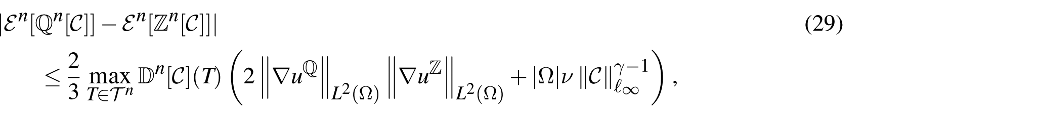
Lemma 6.Fix. For any, we have
where we denotedthe solution of the discrete Poisson equation (18) with permeability, andthe solution of (18) with permeability.
Proof: Using as a test function in the discrete Poisson equation (18) for yields for the kinetic part of (26),
Analogously, we have
Therefore,
Now, using as a test function in the discrete Poisson equation for and vice versa, and subtracting the resulting identities, we obtain
We combine the last two identities and use the Cauchy–Schwarz inequality to estimate
where we also used the uniform bound .
To estimate the difference of the metabolic parts of (26), we use the inequality , which holds for a, and . We obtain
We conclude by using (25). ■
With the uniform -bound (15) on the solutions of the Poisson equation (18) provided by Proposition 1, we readily obtain the following corollary.
Corollary 7.Let,, be a sequence of non-negative conductivities such that
Then
2.3. The continuum energy functional
In this section, we study the properties of the continuum energy functional (5) and its relation to its semi-discrete version (26). We start by proving the continuity of (5) with respect to the norm topology of , .
Lemma 8.Letsatisfy (14) and fix. Let the sequenceconverge toin the norm topology ofas. Then
Proof: Let be a sequence of weak solutions of the Poisson equation (13) with permeability , provided by Proposition 1. Identity (16) gives
Due to the uniform bound (15), there exists , a weak limit of (a subsequence of) , verifying (13) for all test functions . Since strongly in , we can pass to the limit in the weak formulation (13) which establishes u as its weak solution with permeability c and test functions . Again, (16) gives
Combining with (31) we have
which proves the strong continuity of the kinetic part of the energy functional E. The metabolic part is a multiple of the -norm of c; consequently, its strong continuity is obvious. ■
A major observation is that for , the energy functional given by (5) is convex. A proof can be found in [1, Proposition 3.2] or [18, Lemma 6.4]. Then, since is strongly continuous on due to Lemma 8, an application of Mazur’s lemma [25] establishes its weak lower semi-continuity, i.e.,
whenever converges weakly in to c.
Next, we establish an inequality between the semi-discrete and continuum energy functionals restricted to piecewise constant permeabilities on the triangles .
Lemma 9.For anyand non-negative, we have
with the semi-discrete energy functionalgiven by (26) andgiven by (5).
Proof: Let us recall the weak formulation of the discrete Poisson equation (18) with test function ,
Lemma 3 gives
where denotes the constant value of on the triangle , and similarly for and .
Let be the unique weak solution of the Poisson equation (1) with permeability . Using again as a test function gives
Due to the uniqueness (in the respective spaces of functions with vanishing mean) of the solutions of (18) and (1), we have
Then, we have for the kinetic parts of the semi-discrete and continuum energies
where we used the Jensen inequality. Since the metabolic part is identical for both the semi-discrete and continuum energies, we conclude (33). ■
Lemma 10.Let, be a sequence of piecewise constant non-negative conductivitiessuch that. Then
Proof: Using the solution of (13) as a test function, we obtain
On the contrary, using the solution of (18) as a test function, we obtain
Consequently,
where is an -stable interpolator, i.e., Scott–Zhang or Clement. Note that due to the uniform boundedness of in provided by (15), we have
Moreover, using as a test function in the discrete Poisson equation (18) for , we have
where we used Lemma 3 in the first line, recalling that . On the other hand, using as a test function in the Poisson equation (13) for , we obtain
Consequently,
Using again the uniform boundedness of in provided by (15) of Proposition 1, combined with the -stability (35), we conclude. ■
2.4. Γ-convergence of the semi-discrete energy functionals and construction of global energy minimizers
The main result of this section is the Γ-convergence of the sequence of the semi-discrete energy functionals (26) in the appropriate topology.
Theorem 11.Letbe a sequence of non-negative conductivitiessuch thatandweakly- ∗ in. Then
Moreover, for any, there exists a sequenceconverging to c in the norm topology of,, such that
Proof: Statement (36) is a direct consequence of the weak lower semi-continuity (32) of the energy functional , combined with Lemma 10. Indeed, for any , we have
To prove (37), let us fix and construct as the sequence of piecewise constant approximates of c. By standard approximation theory, we then have in the norm topology of for any . Then, the strong continuity of the energy functional with respect to the -topology established in Lemma 8 gives
Moreover, Lemma 9 gives , which directly implies (37). ■
With Theorem 11, it is straightforward to construct global minimizers of the continuum energy (5) as limits of sequences of minimizers of the discrete energy functional (27) on equilateral triangulations.
Theorem 12.Let,, be a sequence of global minimizers of the rescaled discrete energy functionalsgiven by (27). Assume that. Then, up to an eventual selection of a subsequence,converges weakly-* to. Under the additional assumption that, c is a global minimizer of the continuum energy functional (5).
Proof: The uniform boundedness of obviously implies that is uniformly bounded in and (an eventual subsequence) converges weakly-* to some . Then, statement (36) of Theorem 11 gives
We claim that if , then it is a global minimizer of the energy functional (5). For contradiction, let us assume that there exists such that
By averaging over the diamonds , we construct a sequence such that converges to in the norm topology of . Moreover, since , the sequence satisfies the property (30). Corollary 7 and the statement (37) of Theorem 11 gives then
On the contrary, we have
Since by construction we have for all , we finally obtain
which is a contradiction to (38). ■
Finally, let us note that by the standard theory of convex gradient flows on Hilbert spaces, see, e.g., [26,27], we can construct unique weak solutions of the systems (1)–(2). We refer to [1, Section 3.1] for further details.
Proposition 13.Let, satisfying (14) andnon-negative almost everywhere in Ω. Then, the problems (1) –
(4) admit a unique global weak solution, withand satisfying the energy inequality
3. Numerical results
In this section, we briefly discuss some of the details of our numerical implementation. We first introduce the finite element spaces, the semi-discrete nonlinear equations, and their time-advancing scheme and then discuss the linearized equations. We conclude with numerical experiments in Section 3.1 and 3.2. For additional details, see [28].
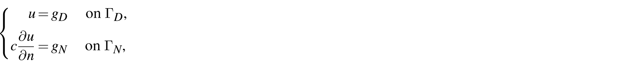
While we used homogeneous Neumann boundary conditions to derive the continuum energy, here we consider the system of equations (1)–(2) closed with more general boundary conditions
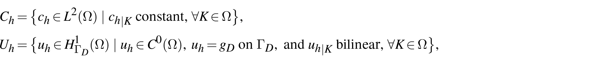
where , with (respectively ) being the subset of the boundary where we may consider non-homogeneous essential (respectively natural) boundary conditions with datum (respectively ). We use finite element spaces consisting of piecewise constant elements for the conductivity and bilinear elements for the pressure in two dimensions, i.e.,
where K is a quadrilateral cell of the tessellated domain Ω.
For the sake of stability and well-posedness, we will use a regularized metabolic cost when
that reduces to when , as initially proposed in Astuto et al. [29].
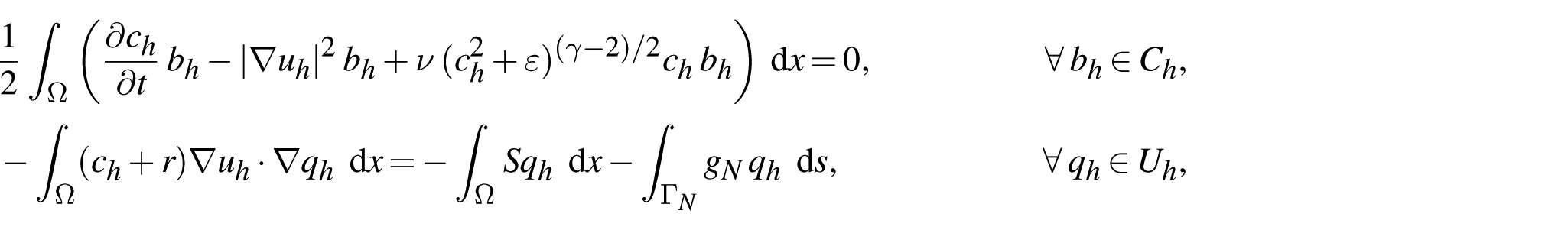
After a simple rescaling to ensure the symmetry of the linearized equations, the variational formulation of the discrete problem reads: given , find , such that, for almost every
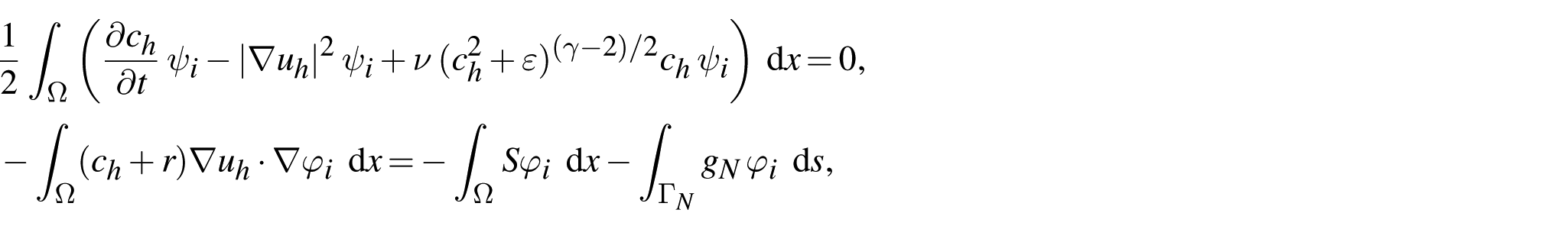
which leads to the set of differential-algebraic equations
where (respectively ) are the test functions for (respectively ).
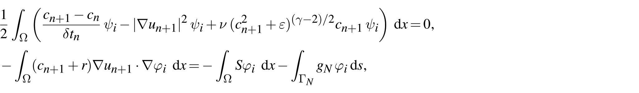
To advance in time, we use the backward Euler scheme, which allows us to preserve the positivity of the conductivity. Dropping the h subscript, we first compute the initial pressure by solving
where is the given initial condition for the conductivity. Denoting by and the finite element approximations for the conductivity and pressure at step n, we then solve the equations
where is the time step.
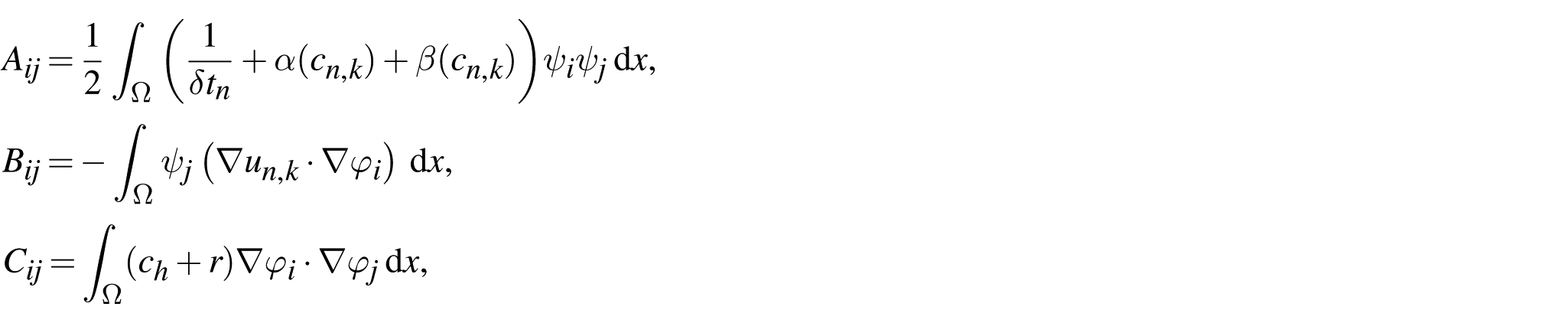
This nonlinear system of equations is solved using the inexact Newton method [30]. The symmetric indefinite Jacobian matrix at a given linearization point is of the form
where
with (respectively ) is the linearization point at the kth Newton step for the conductivity (respectively pressure), and the function coefficients α and β are given by
Note that, when and , A is a symmetric positive definite matrix because
When , the positive definiteness of A cannot be guaranteed unless we make assumptions on the time step.
The matrix J admits the exact factorization
where the Schur complement D can be explicitly assembled since A is a block-diagonal matrix with each block associated with a single element. The inverse factorization requires solving the inexpensive diagonal problem A twice, and the Schur complement system D only once. Numerically, we observed that D is a symmetric positive semi-definite matrix representing a perturbed scalar diffusion problem having the same kernel as the discretized Poisson problem C. Instead of solving the Schur complement system exactly, we can thus use an algebraic multigrid (AMG) preconditioner, which guarantees robustness and has an overall cost that is linear in the matrix size.
The code used to conduct the numerical experiments described in this section is publicly available as a tutorial of the Portable and Extensible Toolkit for Scientific Computing (PETSc, [31]).1 The management of unstructured grids and the implementation of finite elements are based on the DMPLEX infrastructure [32]. Time integration is performed using the TS module [33]; adaptive time stepping is performed using digital filtering-based methods [34] combined with the approximation of the local truncation error using extrapolation. The nonlinear systems of equations arising from the time-advancing schemes are solved with a tight absolute tolerance of 1.E-10; Jacobian linear systems are solved using the right-preconditioned generalized minimal residual (GMRES) method [35], and the Schur complement system is approximatively solved using the application of an AMG preconditioner based on smoothed aggregation [36]. Linear system tolerances are dynamically adjusted using the well-known Eisenstat and Walker trick, which prevents over-solving in the early steps of the Newton process and tightens the accuracy as convergence is approached [37]. The nonlinear time step problems can sometimes be quite challenging to solve; as a safeguard, we cap the maximum number of nonlinear iterations at 10 and shorten the time step if the Newton process stagnates and does not reach convergence within the maximum number of iterations.
3.1. Network formation
In the first numerical experiment, we demonstrate that the scalar model is capable of simulating a network formation process. For this experiment, we consider a unit square domain , homogeneous Neumann boundary conditions (i.e. , ), and the model parameters , , , and . The domain is discretized using a structured quadrilateral mesh with a 512 x 512 cell arrangement, resulting in a total of 263,000 degrees of freedom. The initial conductivity field is the constant function , the simulation is run up to the final time , and we use the Gaussian source
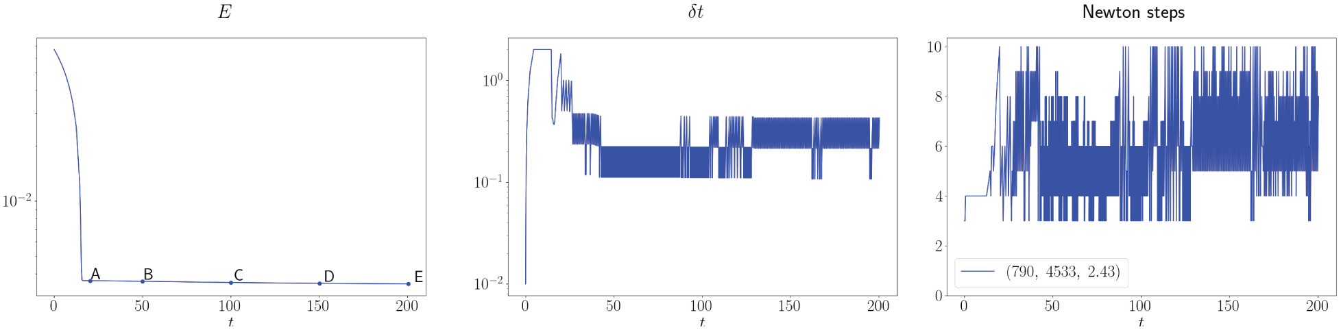
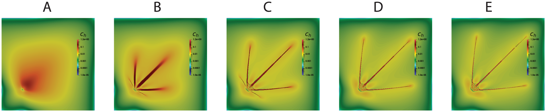
with . Figure 1 presents the system energy E (left panel), the time step size (center), and the number of nonlinear iterations (right) as functions of the simulated time. The legend in the right panel reports the total number of time steps, the total number of Newton steps, and the average number of Krylov iterations per Newton step, providing an overview of the algorithmic costs of the solver. Snapshots of the conductivity field (in logarithmic scale) taken at selected times indicated by the text boxes in Figure 1, are shown in Figure 2.
Network formation: energy (left panel, logarithmic scale), time step (central, logarithmic scale), and number of nonlinear iterations as a function of simulation time for 512 x 512 mesh.
Network formation: conductivity in logarithmic scale at selected time instances as reported at the top of each panel (see Figure 1).
The system energy decreases monotonically throughout the simulation. In the initial phase, the energy decays rapidly as the conductivity field evolves from an initially homogeneous state to a spatially heterogeneous configuration (see panel (a) of Figure 2), allowing relatively large time steps. At this stage, the dynamics are dominated by the minimization of the term . In the subsequent phase, network formation begins (see panels (b) and (c)), driven by the interplay between this positive term and the negative contribution from the metabolic term. During this process, energy variations become smaller, and the solver selects smaller time steps. In the final phase, the energy decreases more slowly toward its steady state, with minimal changes in the conductivity field (see panels (d) and (e)). Overall, the problem exhibits a mild nonlinearity. The backward Euler time advancing scheme encounters a few nonlinear solver failures during the later stages of network formation. Nevertheless, the average number of Krylov iterations per Newton step remains very low, confirming the effectiveness and robustness of the linear preconditioning strategy.
3.2. Solutions of the p-Laplacian equation
We dedicate a substantial portion of the numerical section to the integration of the differential-algebraic equations (1) and (2) up to their steady state, in order to compute solutions of the p-Laplacian equation
with , , , and . To evaluate the approximation properties of the method, we first apply the method of manufactured solutions and compare the numerical results against analytical solutions. Finally, we present experiments demonstrating the robustness of the method for large values of p and non-convex domains.
A priori estimates for the lowest order -conforming finite element discretizations of the p-Laplacian equation with have been established in Ebmeyer and Liu [38] (see also Diening and Ruzicka [39]) in terms of a quasi-norm for convex domains and a sufficiently smooth source term S
where the quasi-norm is defined as
In addition to the quasi-norm, we report convergence rates in terms of the standard Lebesgue norm and the semi-norm of the Sobolev space
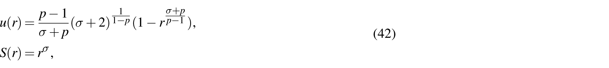
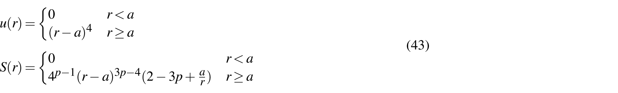
We consider three test cases from Barrett and Liu [40] with radially symmetric smooth functions on the unit square. The first two tests use
with (denoted by TC1) and (TC2) as given in Examples 5.2 and 5.3 in Barrett and Liu [40]. The third test case (denoted by TC3) is also from Barrett and Liu [40] (Example 5.4)
with and . In order to showcase the convergence of the method for larger p-Laplacian exponents, we complement these tests with a fourth one, denoted by TC4, considering (42) with and . For all these tests, we use non-homogeneous essential boundary conditions defined by the analytical solution at the boundary, i.e., and .
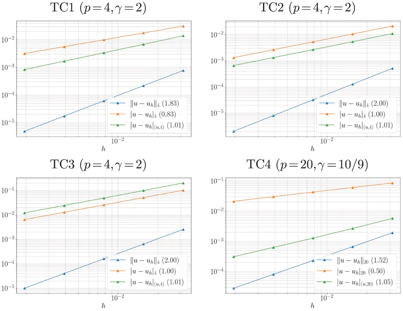
We consider five levels of uniform refinement starting from a uniform grid of elements and report the convergence curves of the final pressures in Figure 3. Optimal first-order convergence in the quasi-norm is obtained in all the cases. Convergence rates in and instead depend on the test case. For TC1, we recover the same convergence rates as in Barrett and Liu [40] (see Table 5.2 in the reference), while our convergence rates for TC2 and TC3 are different than those presented in Tables 5.3 and 5.4 in Barrett and Liu [40] because Barrett and Liu reported the error , where is the finite element method (FEM) interpolant of the exact solution, thus observing superconvergence. The convergence rates in and reported in Figure 3 are in perfect agreement with the best approximation error for linear quadrilateral elements (see, e.g., Corollary 4 in Ainsworth and Kay [41]). For TC1, we have that with , while for TC4 . For TC2 and TC3, we have , and thus, we recover optimal convergence rates using bi-linear elements.
MMS errors and convergence rates (in parentheses) for the test cases TC1, TC2, TC3, and TC4 and different error metrics.
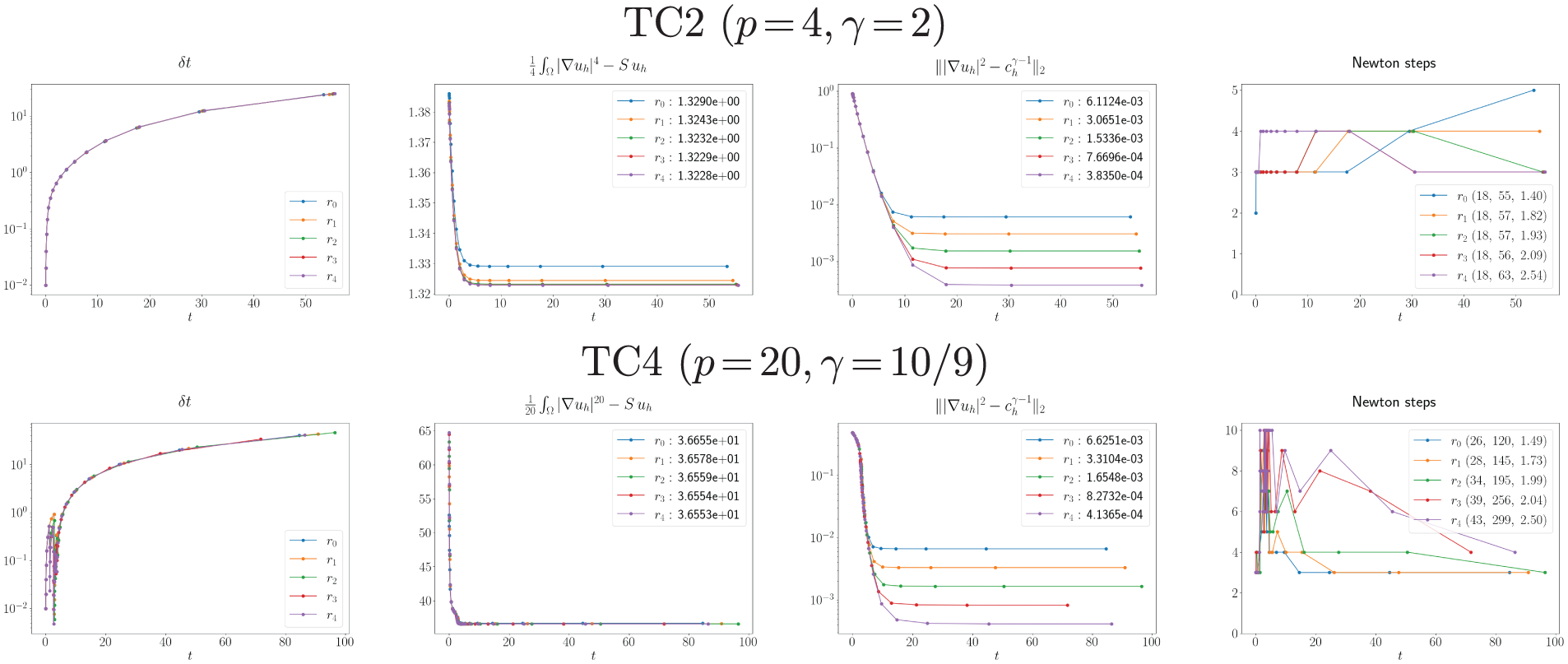
Details on the solution algorithm for the cases TC2 and TC4 are reported in Figure 4; for each time step n, we report, from left to right, the time increment , the p-Laplacian energy , the norm of , and the number of Newton steps as a function of simulation time for the different levels of refinement, from the coarsest , to the finest . The legends in the right panels display the total number of time steps, the total number of Newton steps, and the average number of Krylov iterations per Newton step, providing additional information on the computational costs of the method.
From left to right: time step, p-Laplacian energy (final value in the legend), norm of , and number of Newton steps as a function of time for different levels of uniform refinement r for TC2 (top row) and TC4 (bottom row).
In both test cases, the time step is adaptively adjusted to follow the dynamics of the differential-algebraic equations, which is smoother in the TC2 case. The p-Laplacian energy and decrease over time, with being reduced up to the discretization error because we evaluate the quantity at quadrature points and is not piecewise constant when using bi-linear quadrilateral elements for . For TC2, the number of time steps and the total number of Newton steps remain independent of the refinement level, making the convergence of the method mesh-independent. The linear preconditioning strategy is also highly effective, requiring, on average, only two Krylov iterations per Newton step in all cases. For the TC4 case, time relaxation is more challenging, and a larger value of p leads to stiffer dynamics at all refinement levels. After an initial transient phase, during which the Poisson problem with constant coefficients relaxes smoothly, the increasing nonlinearity of the problem causes the method to enter a second phase that demands a higher number of both time and Newton steps. This occurs because we cannot guarantee the non-negativity of within the nonlinear time step solver, which in turn fails more frequently, resulting in the time step being forced to shrink. Nevertheless, as the mesh is refined, these numbers appear to plateau. To address these challenges, we are currently investigating extensions of our method based on a mass-preserving mixed formulation of the Poisson problem [42]. We are also exploring alternative time-advancing schemes such as pseudo-transient continuation [43], where the rule used to adapt the time step differs fundamentally from the conventional local error–control strategies employed in ODE solvers. This distinction is natural, as the objective of reaching equilibrium as efficiently as possible contrasts with that of accurately tracking a specific trajectory over time.
We now consider a more challenging test case with a non-convex domain and mixed boundary conditions for the pressure, using an analytical solution expressed in polar coordinates
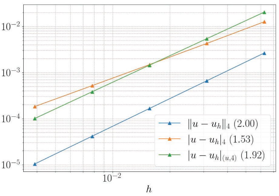
with and . This test case, referred to as TC5, is defined on an L-shaped domain . We impose non-homogeneous essential boundary conditions for the pressure on where the prescribed values are taken from the analytical solution. On the complementary part of the boundary , we enforce non-homogeneous natural boundary conditions with where u is the exact solution. Convergence rates with different levels of uniform refinement are given in Figure 5, showing second-order convergence in the norm and superlinear convergence in the semi-norm and in the quasi-norm .
TC5: MMS errors and convergence rates (in parentheses) for different error metrics.
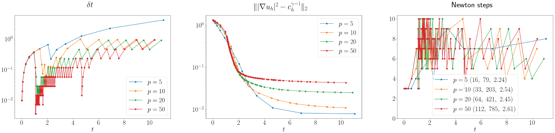
We conclude this section by presenting results for different values of p in a challenging problem without an analytical solution, following the experimental setting of Section 7.3 in Balci et al. [23]. This test, referred to as TC6, considers a constant source term and homogeneous essential boundary conditions for the pressure on the L-shaped domain . The domain is uniformly discretized using 10,000 elements, with mesh size . Solver performance for p-Laplacian exponents (corresponding to ) is reported in Figure 6.
TC6: time step (left panel), norm of (center), and the number of Newton steps (right) as a function of time for different p-Laplacian exponents p.
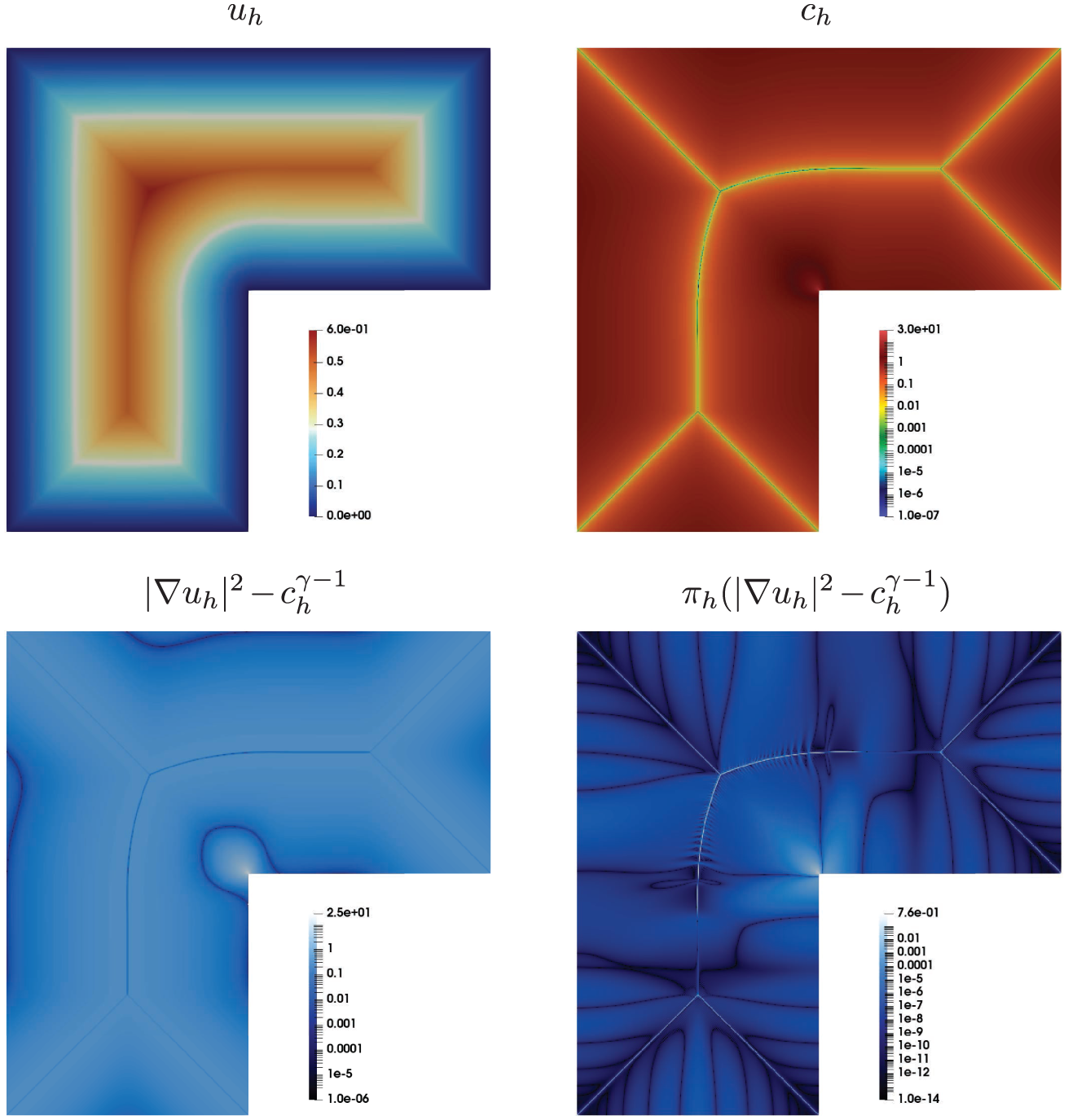
The final values of are larger for larger p, possibly because we did not use a p-dependent norm. The solver is not p-independent overall, as it requires more time and Newton steps as p is increased, due to the increase in nonlinear solver failures. However, the average number of Krylov iterations per Newton step remains essentially constant across all cases, confirming the robustness of the Schur complement-based preconditioner. Figure 7 shows the final states of the pressure and the conductivity for , together with the pointwise error (evaluated in post-processing) and its projection onto , (evaluated within the finite element simulation code). The conductivity (plotted on a logarithmic scale) is small in regions of sharp pressure gradients, where the singularities appear to have Hausdorff dimension one, and attains large values near the concave corner of the domain. These patterns closely resemble the mesh adaptation patterns reported in Figure 7.3 of Balci et al. [23]. The error distribution is nearly uniform across the domain and noticeably larger near the L-shaped corner; the projection of the error is small everywhere in the domain and slightly larger near the corner and where . We remark that a small regularization parameter, , was introduced to ensure convergence of the solver for and . This small level of regularization does not affect the numerical approximation properties, as the region of the domain where has Hausdorff dimension one. Future work will focus on adaptive mesh refinement strategies and the development of error indicators tailored explicitly to the differential-algebraic transient dynamics of the solver.
Top row: final state for pressure (left) and conductivity (right) for the TC6 test case with (corresponding to ).
Footnotes
Acknowledgements
We are thankful for the computing resources of the Supercomputing Laboratory at King Abdullah University of Science and Technology and, in particular, the Shaheen3 supercomputer.
ORCID iD
Stefano Zampini
Funding
The authors disclosed receipt of the following financial support for the research, authorship, and/or publication of this article: The research reported in this paper was funded by King Abdullah University of Science and Technology.
Declaration of conflicting interests
The authors declared no potential conflicts of interest with respect to the research, authorship, and/or publication of this article.
Notes
References
1.
HaskovecJMarkowichPPilliG. Tensor PDE model of biological network formation. Commun Math Sci2022; 20: 1173–1191.
HaskovecJMarkowichPPerthameB. Mathematical analysis of a PDE system for biological network formation. Commun Part Diff Eq2015; 40(5): 918–956.
4.
HaskovecJMarkowichPPortaroS. Emergence of biological transportation networks as a self-regulated process. Discrete Continuous Dyn Syst2023; 43: 1499–1515.
5.
HuDCaiD. Adaptation and optimization of biological transport networks. Phys Rev Lett2013; 111: 138701.
6.
HuDCaiD. An optimization principle for initiation and adaptation of biological transport networks. Commun Math Sci2019; 17(5): 1427.
7.
HaskovecJMarkowichPPerthameB, et al. Notes on a PDE system for biological network formation. Nonlin Anal2016; 138: 127–155.
8.
AlbiGBurgerMHaskovecJ, et al. Continuum modelling of biological network formation. In: BellomoNDegondPTamdorE (eds) Active particles vol. I - theory, models, applications, Modelling and Simulation in Science and Technology. Boston, MA: Birkhäuser-Springer, 2017, pp. 1–48.
9.
AlbiGArtinaMFornasierM, et al. Biological transportation networks: modeling and simulation. Anal Appl2016; 14(1): 185–206.
10.
LiB. Uniqueness of classical solution to an elliptic-parabolic system in biological network formation. J Phys Conf Ser2018; 1053: 012024.
11.
XuX. Regularity theorems for a biological network formulation model in two space dimensions. Kinet Relat Mod2018; 11(2): 397–408.
12.
XuX. Partial regularity of weak solutions and life-span of smooth solutions to a biological network formulation model. SN Partial Differ Equ Appl2020; 1: 18.
13.
BurgerMHaskovecJMarkowichP, et al. A mesoscopic model of biological transportation networks. Comm Math Sci2019; 17(5): 1213–1234.
14.
HaskovecJKreusserLMMarkowichP. Rigorous continuum limit for the discrete network formation problem. Commun Part Diff Eq2019; 44(11): 1159–1185.
15.
HaskovecJMarkowichPPilliG. Murray’s law for discrete and continuum models of biological networks. Math Models Methods Appl Sci2019; 29: 2359–2376.
16.
HuD. Optimization, adaptation, and initialization of biological transport networks. Notes from lecture, 2013.
17.
HaskovecJKreusserLMMarkowichP. ODE and PDE based modeling of biological transportation networks. Commun Math Sci2019; 17(5): 1235–1256.
18.
AlvesNHaskovecJ. Rigorous dense graph limit of a model for biological transportation networks. arXiv [preprint]2025. DOI: 10.48550/arXiv.2507.15829.
LoiselS. Efficient algorithms for solving the p-Laplacian in polynomial time. Numer Math2020; 146(2): 369–400.
21.
CaliariMZuccherS. Quasi-Newton minimization for the p(x)-Laplacian problem. J Comput Appl Math2017; 309: 122–131.
22.
DieningLFornasierMTomasiR, et al. A relaxed Kačanov iteration for the p-Poisson problem. Numer Math2020; 145(1): 1–34.
23.
BalciAKDieningLStornJ. Relaxed Kačanov scheme for the p-Laplacian with large exponent. SIAM J Numer Anal2023; 61(6): 2775–2794.
24.
BartelsSDieningLNochettoRH. Unconditional stability of semi-implicit discretizations of singular flows. SIAM J Numer Anal2018; 56(3): 1896–1914.
25.
RockafellarRT. Monotone operators and the proximal point algorithm. SIAM J Control Optim1976; 14(5): 877–898.
26.
AmbrosioLGigliNSavaréG. Gradient flows in metric spaces and in the space of probability measures. Basel; Boston, MA; Berlin: Birkhäuser Verlag, 2005.
27.
SantambrogioF. Euclidean, metric, and Wasserstein gradient flows: an overview. Bull Math Sci2017; 7: 87–154.
28.
HaskovecJMarkowichPPortaroS, et al. Robust and scalable nonlinear solvers for finite element discretizations of biological transportation networks. arXiv [preprint]2025. DOI: 10.48550/arXiv.2504. 04447.
29.
AstutoCBoffiDHaskovecJ, et al. Asymmetry and condition number of an elliptic-parabolic system for biological network formation. Commun Appl Math Comput2025; 7(1): 78–94.
30.
NocedalJWrightSJ. Numerical optimization. New York: Springer, 2006.
31.
BalayS, et al. PETSc/TAO users manual revision 3.23 (ANL-21/39 rev 3.23,). Argonne, IL: Argonne National Laboratory, 2025.
32.
KnepleyMGKarpeevDA. Mesh algorithms for PDE with Sieve I: mesh distribution. Sci Program2009; 17(3): 215–230.
33.
AbhyankarSBrownJConstantinescuEM, et al. PETSc/TS: a modern scalable ODE/DAE solver library. arXiv [preprint]2018. DOI: 10.48550/arXiv.1806.01437.
34.
SöderlindG. Digital filters in adaptive time-stepping. ACM Trans Math Softw2003; 29(1): 1–26.
35.
SaadYSchultzMH. GMRES: a generalized minimal residual algorithm for solving nonsymmetric linear systems. SIAM J Sci Stat Comput1986; 7(3): 856–869.
36.
AdamsMBrezinaMHuJ, et al. Parallel multigrid smoothing: polynomial versus Gauss–Seidel. J Comput Phys2003; 188(2): 593–610.
37.
EisenstatSCWalkerHF. Choosing the forcing terms in an inexact Newton method. SIAM J Sci Comput1996; 17(1): 16–32.
38.
EbmeyerCLiuWB. Quasi-Norm interpolation error estimates for the piecewise linear finite element approximation of p-Laplacian problems. Numer Math2005; 100: 233–258.
39.
DieningLRuzickaM. Interpolation operators in Orlicz–Sobolev spaces. Numer Math2007; 107(1): 107–129.
40.
BarrettJWLiuWB. Finite element approximation of the p-Laplacian. Math Comp1993; 61(204): 523–537.
41.
AinsworthMKayD. Approximation theory for the hp-version finite element method and application to the non-linear Laplacian. Appl Numer Math2000; 34(4): 329–344.
42.
BoffiDBrezziFFortinM. Mixed finite element methods and applications, vol. 44. Heidelberg: Springer, 2013.