We consider a frame-indifferent variational model for magnetoelastic solids in the large-strain setting with the magnetization field defined on the unknown deformed configuration. Through a simultaneous linearization of the deformation and sharp-interface limit of the magnetization with respect to the easy axes, performed in terms of Γ-convergence, we identify a variational model describing the formation of domain structures and accounting for magnetostriction in the small-strain setting. Our analysis incorporates the effect of magnetic fields and, for uniaxial materials, ensures the regularity of minimizers of the effective energy.
In the modeling of deformable ferromagnets, magnetostriction refers to the effect for which mechanical and magnetic responses of materials influence each other. Nowadays, this effect is largely exploited in the design of many technological devices such as sensors and actuators [1, 2]. In this regard, specific rare-earth and shape-memory alloys (e.g., TerFeNOL and NiMnGa) have been found of great interest in view of their ability of undergoing remarkably large deformations upon the application of relatively moderate magnetic field, which is often referred to as giant magnetostriction [3].
Magnetocrystalline anisotropy, i.e., the existence of preferred directions of magnetization (called easy axes) determined by the underlying lattice structure of materials, plays a key role in the mechanism behind magnetostriction. In the absence of external stimuli, magnetic materials spontaneously arrange themselves in regions of uniform magnetization (called Weiss domains) separated by thin transition layers (called Bloch walls) [4]. The application of an external magnetic field leads to a reorganization of the domain structure mainly due to the more favorable orientation of certain easy axes with respect to the magnetic field. The movement of domains results in a macroscopic strain, thus inducing a deformation of the material. For a comprehensive treatment of the physics of magnetoelastic interactions, we refer, e.g., to the books of Brown [5], Landau and Lifshitz [6].
Providing an effective description for the emergence of domain structures accounting for mechanical stresses in precise mathematical terms appears to be a very challenging task. This study constitutes an attempt in this direction by means of variational methods. Starting from a large-strain model for magnetostrictive solids, we study the asymptotic behavior of the energy for infinitesimal strains and for magnetization aligning with the easy axes. In this way, we identify an effective model accounting for the linearized elastic energy and the formation of domain structures. Our main results are outlined in subsection 1.4 below.
1.2. The variational model
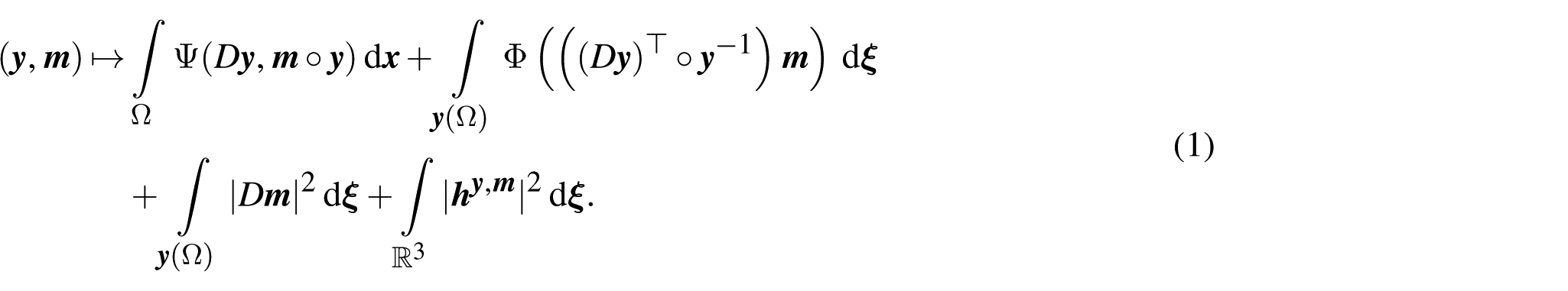
In this work, we adopt the variational model of magnetoelasticity due to Brown [5, 7]. A magnetoelastic body is subjected to a deformation , where represents its reference configuration, and a magnetization field . The latter is understood as the average of magnetic dipoles per unit volume. Hence, the saturation constraint [5, p. 73] requires in . The magnetoelastic energy reads
The first term in (1) accounts for the elastic energy and involves a material density Ψ which exhibits the coupling between magnetization and deformation gradient. The prototypical example takes the form
where W is an auxiliary density and represents the spontaneous strain corresponding to z. For instance, magnetostriction often induces an elongation along the magnetization direction [8, 9], which can be modeled as
by choosing .
The second term in (1) stands for the anisotropy energy. The density Φ is nonnegative and vanishes exactly in the direction of the easy axes, thus favoring their attainment. For instance, in the case of uniaxial materials,
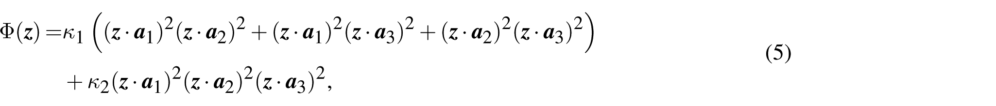
with being the easy axis and , while for cubic materials,
where are the mutually orthogonal easy axes, , and . The easy axes are determined by the undistorted lattice structure in the reference configuration. In this model, these axes are transported to the deformed configuration via the Cauchy–Born rule [10]. For densities Φ depending on the direction cosines, such as those in (4)–(5), this assumption explains the term multiplying m in (1). The third term in (1) constitutes the exchange energy which favors a constant magnetization of the specimen. More generally, the norm squared could be replaced by a quadratic form in the magnetization gradient.
Eventually, the fourth term in (1) stands for the magnetostatic self-energy related to the long-range interactions. In absence of external currents, the stray field solves the Maxwell system
We remark that, when Ψ is invariant under left-multiplication by rotation matrices (see, e.g., [8, Equation (20)]), the energy in (1) fulfills the principle of frame indifference. In particular, this happens for (2)–(3) when the same property is satisfied by W. In this regard, we highlight that the dependence of the anisotropy energy on the deformation gradient (see, e.g., [8, Equation (21)]) remains crucial for frame indifference. Additionally, the energy is invariant upon replacing m with .
Equilibrium configurations correspond to minimizers of the energy (1). The minimization becomes nontrivial once the deformation y is prescribed on a portion of the boundary or applied loads are considered. In presence of an external field f, the corresponding energy contribution reads
1.3. Review of the most relevant literature
To put our findings into context, we briefly review the most relevant literature. Without any claim of completeness, we only mention a few works concerning the model outlined in subsection 1.2 that are related to our work.
The existence of minimizers for the functional (1) has been investigated in [11–15] under various regularity assumptions on admissible deformations. The papers [12, 13, 15] address also the existence of quasistatic evolution in the rate-independent setting. Other results of this kind have been achieved in previous works [16–18] for a similar model of nematic elastomers. Note that in all these studies the anisotropy energy is either assumed to be independent on the deformation gradient [13, Equation (1.2)] or entirely neglected. Indeed, according to (1), the anisotropy contribution constitutes a leading-order term of the functional whose lower semicontinuity cannot be guaranteed when Φ is nonconvex such as in (4)–(5).
The linearization of the energy (1) has been rigorously performed in the work by Almi et al. [19], thus recovering a well-established magnetoelasticity model for the small-strain setting [20]. For rigid bodies, the sharp-interface limit of magnetizations toward the easy axes has been addressed by Anzellotti et al. [21]. The case of deformable bodies has been tackled in the papers by Grandi and co-authors [22, 23]. More precisely, these works concern multiphase solids with Eulerian interfaces but, as mentioned in [23, p. 411], their analysis can be reformulated in terms of the model in subsection 1.2 by interpreting the diffuse phase indicators as magnetization fields. Still, the dependence of the anisotropy energy on the deformation gradient is dropped in these two works, so that the model does not comply with frame indifference. All above-mentioned results for the linearization and the sharp-interface limit are stated in terms of Γ-convergence [24, 25].
Although not directly relevant for our study, we also mention the derivation of effective models, still by Γ-convergence, in the direction of dimension reduction [26, 27] and relaxation [28, 29].
1.4. Contributions of the paper
In this paper, we rigorously derive a variational model describing the formation of domain structures and accounting for magnetostriction in the small-strain regime. The derivation is performed in the sense of Γ-convergence through a simultaneous linearization of deformations and sharp-interface limit of magnetizations with respect to the easy axes. Our main results are given in Theorem 2.1, Theorem 2.2, and Theorem 2.4. Here, we limit ourselves in briefly outlining their content and we refer to section 2 for their precise statement.
We adopt the functional setting of Barchiesi et al. [11]. Deformations are modeled as maps with satisfying the divergence identities (see Definition 3.3 below), which is equivalent to excluding cavitation. Thus, by replacing the deformed configuration with the topological image (see Definition 3.2 below), we can define magnetizations as Sobolev maps on this set, which in turn allows for a meaningful definition of the magnetoelastic energy (1).
For a small parameter , we consider a rescaled version of the magnetoelastic energy (see (7)–(9) beylow). Specifically, the elastic term is rescaled by and the elastic density takes the form in (2) with the spontaneous strain of magnetizations (i.e., the term in (8) below) given by a perturbation of the identity of order ε (see (10) below); anisotropy and exchange term are rescaled similarly to the classical Modica–Mortola functional [30] in terms of a power with
where specifies the growth of W with respect to the determinant of its argument (see assumption (W5) below); eventually, we neglect the stray-field term. Condition (6) is commented in subsection 1.5 below.
Theorem 2.1 shows that the sequence enjoys suitable compactness properties or, in the terminology of Γ-convergence, that this sequence is equi-coercive (see, e.g., [25, Definition 7.6]). Limiting states are determined by infinitesimal displacements and magnetizations which attain only the easy axes (up to sign). Thus, each limiting magnetization determines a domain structure.
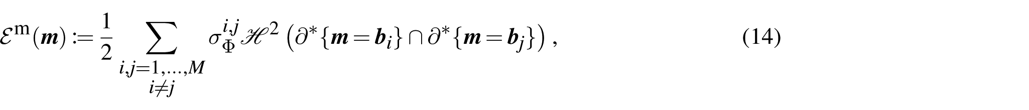
Theorem 2.2 provides the Γ-limit of the sequence , as . The functional is the sum of two contributions (see (12)–(14) below): a linearized elastic energy where the strain corresponding to stress-free configuration is quadratic in the magnetization, and an energy measuring the area of the interfaces between different magnetic domains that resemble the classical Γ-limit of the vectorial Modica–Mortola functional [30]. The elastic contribution coincides with the one commonly adopted in small-strain models [20], while the magnetic one agrees with the sharp-interface limit identified in [21].
From Theorem 2.1 and Theorem 2.2, we immediately deduce the convergence of almost minimizers by standard Γ-convergence arguments (see, e.g., [25, Theorem 7.8]). As the contributions given by stray and external fields are both continuous with respect to the relevant notion of convergence, these are easily incorporated (see, e.g., [24, Remark 1.7]). The convergence result for almost minimizers is given in Corollary 2.3.
Eventually, Theorem 2.4 addresses the regularity of minimizers of the functional in the case of uniaxial materials as in (4). For sufficiently regular boundary datum and external field, we prove the regularity of the infinitesimal displacement and the boundaries of magnetic domains. This result provides a slight extension of [21, Theorem 5.1] which accounts for magnetostriction in the small-strain setting.
1.5. Comments and outlook
Our main findings represent the first results combining linearization and sharp-interface limit for Eulerian-Lagrangian energies, i.e., energies comprising both terms in the reference configuration and in the unknown deformed configuration.
The expression of the spontaneous strain of magnetizations postulated here (see (10) below) is evidenced in the literature (see, e.g., [8, Equation (90)]) and seems more natural compared with the one in previous work [19], even though the two are asymptotically equivalent. In contrast with previous works [22, 23], the anisotropy energy depends on the deformation gradient, so that our diffuse-interface model complies with frame indifference. In this regard, the rigidity of the model arising from the linearization process is steadily exploited while handling this additional dependence on the deformation gradient.
From a technical point of view, we observe that is assumed in previous works [19, 22, 23], while here we only require . Thus, admissible deformations are possibly discontinuous in our setting. The consequent difficulties are overcome by means of the techniques developed in previous works [11, 12, 14]. In this regard, excluding cavitation is essential not only for a consistent definition of energy functionals on the deformed configuration, but also for analytical reasons. Indeed, this setting ensures that geometric image (see Definition 3.1 below) and topological image of deformations coincide up to negligible set (see Proposition 3.4 below), which justifies the change-of-variable formulas used throughout the proofs.
Condition (6) identifies the regime where no interaction between elastic and magnetic energy terms occurs during the process of Γ-limit. As a result, the magnetic term of the limiting energy is independent of the displacement. This decoupling simplifies the proofs significantly. Different regimes potentially leading to a Γ-limit where the magnetic term depends also on the displacement will be the subject of future investigations.
Other interesting and ambitious directions might concern the linearization for spontaneous strains of magnetizations that are not perturbations of the identity, and the sharp-interface limit at large strains with the anisotropy energy depending on the deformation gradient.
1.6. Structure of the paper
The paper is organized into four sections. Section 1 constitutes this introduction. In section 2, we specify the setting of our problem and we state our main findings. Section 3 collects results from the literature that will be needed for the proofs of our main results presented in section 4.
1.7. Notation
Given , we employ the notation and . We work in with denoting the unit sphere centered at the origin. The class of square matrices is endowed with the Frobenius norm. The symbol id is used for the identity map on , while I and O denote the identity and the null matrix in . Given , we write for its determinant and for its transpose. is the set of matrices with positive determinant, while is the set of rotations. stands for the class of symmetric matrices and is the symmetric part of . We write for the symmetric difference of two sets .
The Lebesgue measure and the two-dimensional Hausdorff measure on are denoted by and , respectively. The expressions “almost everywhere” (abbreviated as “a.e.” within the formulas) as well as the adjective “negligible” always refer to the Lebesgue measure. The symbol is employed for the indicator function of a set . We use standard notation for Lebesgue spaces (), spaces of differentiable and Hölder functions ( and ), Sobolev spaces (), and spaces of functions with bounded variation (BV). The subscripts “loc” and “c” are used for their local and compactly supported versions. Domain and codomain are separated by a semicolon, and the codomain is omitted for scalar-valued maps. We write for the measure with density g with respect to . Lebesgue spaces on boundaries are always meant with respect to . Given , we write . Distributional gradients are indicated by D, while E is used for symmetrized gradients. Boundary conditions for Sobolev functions are always understood in the sense of traces. Given a map w with bounded variation, we write and for its total variation and jump set, respectively. Eventually, the class of sets of locally finite perimeter in is written as with denoting the reduced boundary of . Thus, stands for the relative perimeter of E in an open set .
We adopt the usual convention of denoting by C a positive constant depending on known quantities (in particular, independent on ε) whose value can change from line to line.
2. Setting and main results
2.1. Setting
Throughout the paper, we fix
The fact that Δ has Lipschitz boundary in is understood in the sense of [31, Definition 2.1].
Fix . For each , we consider the functional
with
defined on the class of admissible states
where
The divergence identities (DIV), introduced in [32], are given in Definition 3.3 below. Intuitively, the validity of these identities excludes the phenomenon of cavitation [33]. Recall that y is termed almost everywhere injective whenever the restriction of y to the complement of a negligible subset of Ω is an injective map [34].
The elastic energy (8) depends on a material density on which we make the following assumptions:
(W1) Orientation preservation: if and only if ;
(W2) Regularity: W is continuous on and of class in a neighborhood of ;
(W3) Frame indifference: W is frame indifferent, i.e.,
(W4) Ground state: ;
(W5) Growth: there exist a constant such that
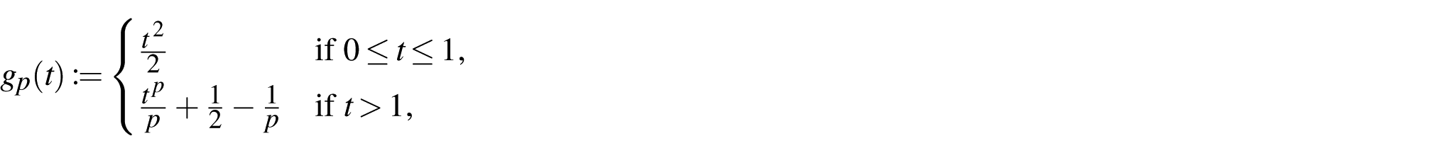
where and are defined as
and
The specific expressions of the functions and are not relevant as long as is bounded from below by , and goes as for and controls for . The tensor field appearing in (8) is defined as
with and , where . This tensor is invertible and its inverse reads as
The magnetic energy (9) is given by the sum of two integrals on the topological image of Ω under y. This set was introduced in [11] and it is here recalled in Definition 3.2 below. The first integral features the function which is assumed to satisfy:
(Φ1) Multiple wells: There exist with and distinct elements such that ;
(Φ2) Regularity: Φ is continuous on and of class in a neighborhood of .
From the modeling point of view, in (Φ1) we should take with , for , and for where denote the easy axes. However, this fact is not relevant for the present analysis.
By passing, we also remark that the energy in (7)–(9) is frame indifferent in view of (W3) and the objectivity of , that is,
The limit functional
with
is defined on the class
In (13), the quadratic form is defined as
where the elasticity tensor is defined as the differential of W at the identity, is the symmetrized gradient of u, and, as in (3), we define by setting
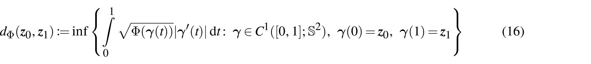
Moreover, we set
where denotes the geodesic distance defined by
for all .
2.2. Main results
Our main results show that the asymptotic behavior of the functionals , as , is effectively described by the functional in the regime (6). In this setting, each of the two functionals in (13) and (14) is the Γ-limit of the corresponding term in (8) and (9).
The first result ensures that the sequence enjoys suitable compactness properties.
Theorem 2.1 (Compactness). Assume (W1)–(W5), (Φ1)–(Φ2), and (6). Letbe a sequence withfor all. Suppose that
Then, there existssuch that, up to subsequences, we have as
The second result shows that the functional provides an optimal lower bound for . For the notion of Γ-convergence, we refer to [24, 25].
Theorem 2.2 (Γ -convergence). Assume (W1)–(W5), (Φ1)–(Φ2), and (6). Then, the sequence-converges to the functional, as, with respect to the convergences in Theorem 2.1. Namely, the following two conditions hold:
(i) Lower bound: For any sequencewithfor alland anyfor which (18) – (21) hold true, we have
(ii) Optimality of the lower bound: For any, there exists a sequencewithfor allfor which (18) – (21) hold true and we have
The effect of magnetic fields can be easily incorporated within our analysis. Following [7], we define the stray field corresponding to a deformation and a magnetization as the unique distributional solution to the Maxwell system
where denotes the inverse of y as given in Proposition 3.5 below. As a consequence of Proposition 4.1 below, existence and uniqueness of the stray field are guaranteed in our setting, and the associated energy contribution
is well defined. Additionally, the work of the applied magnetic field is accounted by the Zeeman energy functional
For a fixed constant , we define the total energies
and
It turns out that the functionals and constitute continuous perturbations with respect to the relevant topology. Therefore, standard Γ-convergence arguments (see, e.g., [24, Remark 1.7]) yield the following statement for sequences of almost minimizers.
Corollary 2.3 (Convergence of almost minimizers). Assume (W1)–(W5), (Φ1)–(Φ2), and (6). Letbe a sequence withfor allsatisfying
where we set. Then, there existssuch that, up to subsequences, (18)–(21) hold true andis a minimizer ofwith
Eventually, we discuss the regularity of minimizers for the limiting energy in a special case. For simplicity, as in [21], we discuss only the interior regularity in the case . This setting can describe uniaxial materials with Φ as in (4) by choosing and . In this situation, the limiting magnetic energy (14) can be trivially rewritten as
Therefore, we can resort to the regularity theory for sets with minimal perimeter [35].
Theorem 2.4 (Regularity of minimizers). Letbe a minimizer of the functional. Then,for all. Additionally, assume. Ifwith, then the setis a surface of classin Ω. Furthermore, ifwith, then.
3. Preliminary results
In this section, we collect some preliminary notions and facts that will be instrumental for the proofs of the results in section 2.
3.1. Geometric and topological image
We introduce two concepts of image for deformations, namely that of geometric and topological images. For the notions of approximate differentiability and density of a set, we refer to [36].
Definition 3.1 (Geometric image). Letwithfor almost all. The geometric domainofyis defined as the set of pointsat whichyis approximately differentiable withand there exist a compact setwith density one atxand a mapsuch thatand. Moreover, for any measurable set, the geometric image ofAunderyis defined as.
From [37, pp. 582–583], we known that has full measure in Ω. The technical condition expressed in terms of w is included in the definition just for convenience as it ensures that is (everywhere) injective [37, Lemma 3]. Hence, we can consider the inverse of y as the map .
Below, will denote the precise representative of the map defined as
In loose terms, the restriction of to the boundary of almost every set is continuous as a consequence of the assumption and Morrey’s embedding. This observation allows for a notion of topological degree for Sobolev mappings. For the degree of continuous functions, we refer to [38]. The next definition exploits the sole dependence of the degree on boundary values.
Definition 3.2 (Topological image). Letandbe a domain such that. The topological image ofUunderyis defined as
wheredenotes the topological degree of any extension oftoat the pointξ. Moreover, the topological image of Ω underyis defined as
By classical properties of the topological degree (see, e.g., [14, Remark 2.17]), is a bounded open set. The set is thus open but possibly unbounded.
3.2. Divergence identities
The divergence identities are a generalization of the identity , asserting that the distributional and pointwise determinant coincide [39], which has been investigated in connection with the weak continuity of the Jacobian determinant [32].
Definition 3.3 (Divergence identities). Let. The mapyis termed to satisfy the divergence identities (DIV) whenever
where the divergence on the left-hand side and the equality are understood in the sense of distributions over Ω. Namely,
for alland.
Let us remark that satisfying the divergence identities is equivalent to having zero surface energy in the setting of [11, 40].
We state two consequences of the divergence identities. The first result shows that geometric and topological images actually coincide and, in turn, rule out the phenomenon of cavitation.
Proposition 3.4 (Excluding cavitation). Letwithsatisfy (DIV). Then,up to negligible sets. That is,.
The second result concerns the inverse of deformations. As already noted, if y is almost everywhere injective, then the restriction is actually (everywhere) injective. Thus, the inverse yields an almost everywhere defined map on the open set in view of Proposition 3.4. The next results assert its Sobolev regularity.
Proposition 3.5 (Regularity of the inverse). Letwithbe almost everywhere injective and satisfy (DIV). Then,withalmost everywhere in.
Proof. From [11, Proposition 5.3], we know that and the inverse formula holds. Moreover,
and
thanks to Proposition 3.4, the inverse formula, and the change-of-variable formula, where the last integral is finite since . □
3.3. Least upper bound of positive measures
Let be an open set and let be a finite family of positive Borel measures on U. The least upper bound of is defined for every Borel set by setting
This is also a positive Borel measure, namely, the smallest positive Borel measure on U with the property that for any Borel set [36, p. 31]. In particular, as noted in [36, Remark 1.69], for absolutely continuous measures, one has
The following lower semicontinuity result will be employed in the proof of Theorem 2.2(i).
Lemma 3.6 (Lower semicontinuity of the least upper bound of total variations). Letbe an open set and, for each, letbe a sequence inandsuch thatin, as. Then,
Proof. Let be a Borel partition of U. By the lower semicontinuity of the total variation,
Thus
The claim follows by taking the supremum among all Borel partitions of U. □
4. Proofs
In this section, we prove the main results stated in section 2.
4.1. Compactness result
We begin by proving our compactness result. Below, we will consider the first-order Taylor expansion of Φ. For fixed , we have
where , as . For , we define
so that
in view of (Φ2). Additionally, for , we define by setting
where is given by (16).
Proof of Theorem 2.1. We subdivide the proof into three steps.
Step 1 (Compactness of deformations and displacements). For convenience, we set , and , where we adopt the notation in (10). From (17) and assumption (W5), we obtain
Given that for all , the previous estimate implies in . Thus, the sequence is bounded in . Noting that for all , where we employ (10) and (15), and computing
the triangle inequality gives
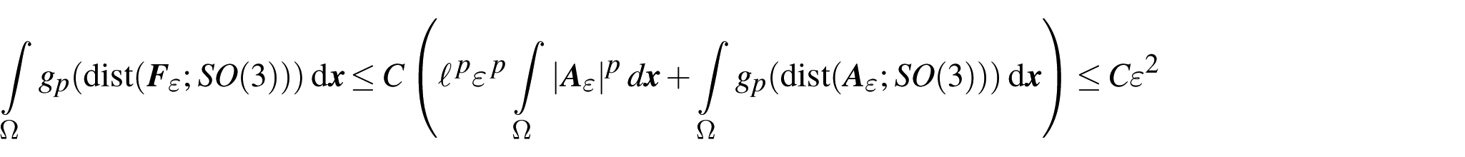
The estimates (32) and (34) together with the monotonicity of and the elementary inequality
yield
given that . As
from the last estimate we obtain
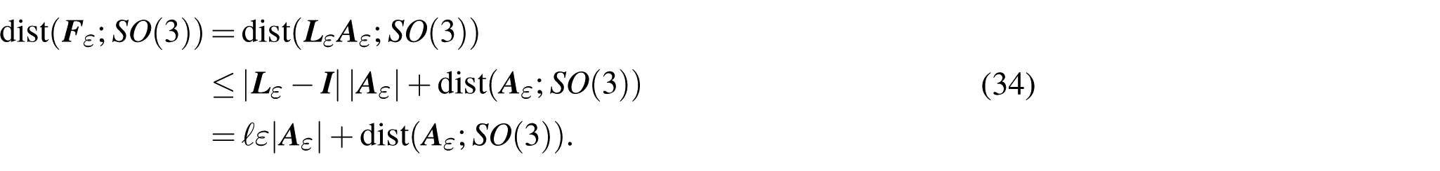
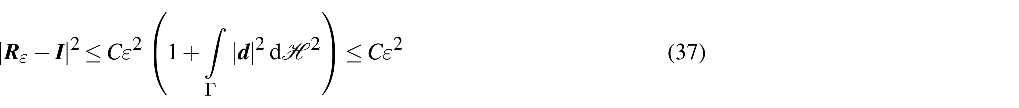
Let and . First, we show that is bounded in . Then, by applying the Poincaré inequality with trace term, we find for which (19) holds along a not relabeled subsequence. In particular, on Δ owing to the weak continuity of the trace operator. From (35), using the classical rigidity estimate [41, Theorem 3.1] (see also [26, Remark 2.3] and [42, Section 2.4]), we identify a sequence in satisfying
Then, by arguing as in [43, Proposition 3.4], taking advantage of the boundary condition on Δ, we establish
and, in turn,
This proves the claim.
Next, we check that in . Then, (18) follows once again thanks to the Poincaré inequality. We argue as in [19, Lemma 3.3] and we estimate
The first integral on the right-hand side is bounded by (36), while for the second one we estimate
thanks to (37). Altogether, we find
which yields the desired convergence.
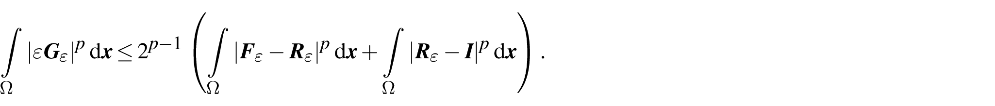
Furthermore, we claim that
so that, by applying [12, Proposition 2.23(ii)], we obtain
Note that
where . Hence, as , we have
Using the elementary estimate
together with (32), we deduce
Thus, is bounded in . In view of (18), we also know that almost everywhere in Ω for a not relabeled subsequence. Therefore, (38) follows by Vitali’s convergence theorem and Urysohn’s property.
Step 2 (Compactness of magnetizations). We fix an exponent satisfying
noting that such a choice is always possible in view of (6). Let . By Chebyshev’s inequality,
Recall that
where each is a homogeneous polynomial of degree k in the entries of G and, as such,
Thus, recalling (43), we have
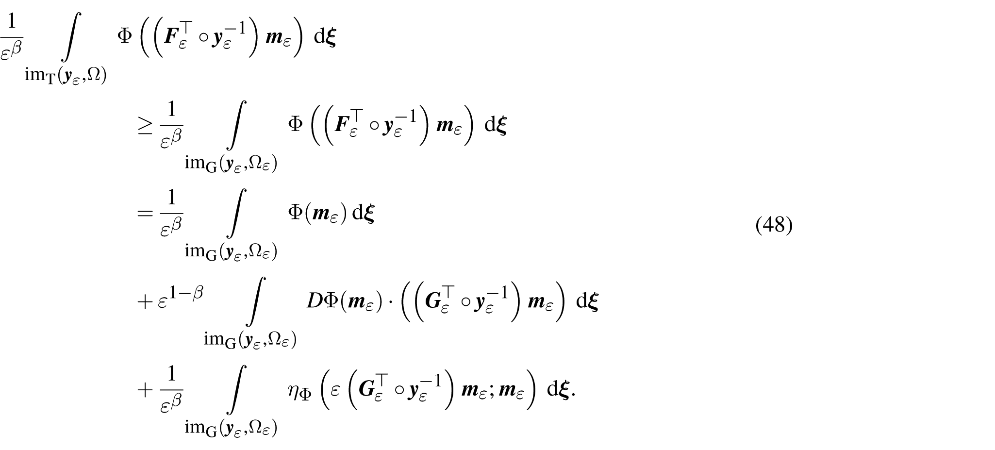
By considering the Taylor expansion of Φ around as in (29) and Proposition 3.4, we write
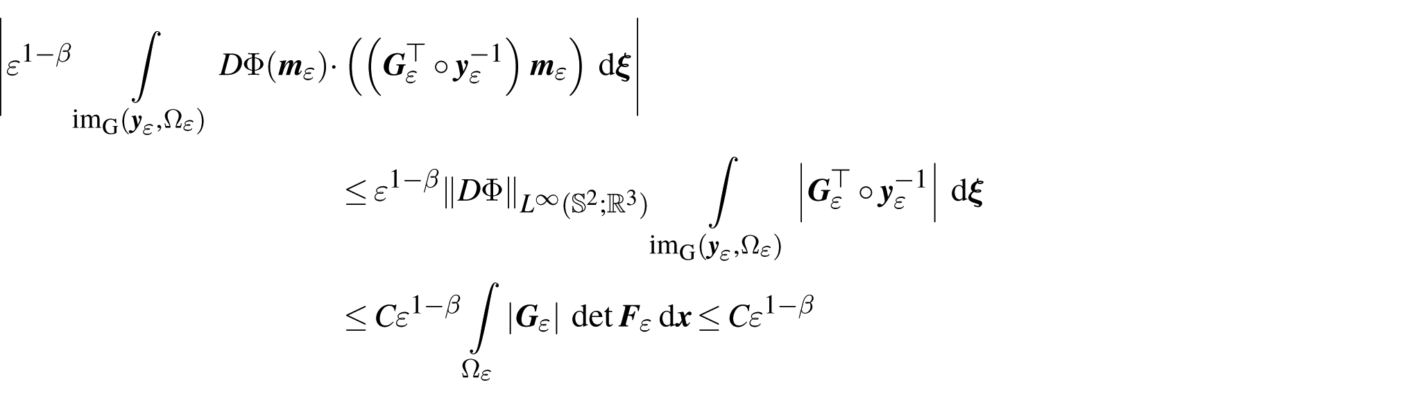
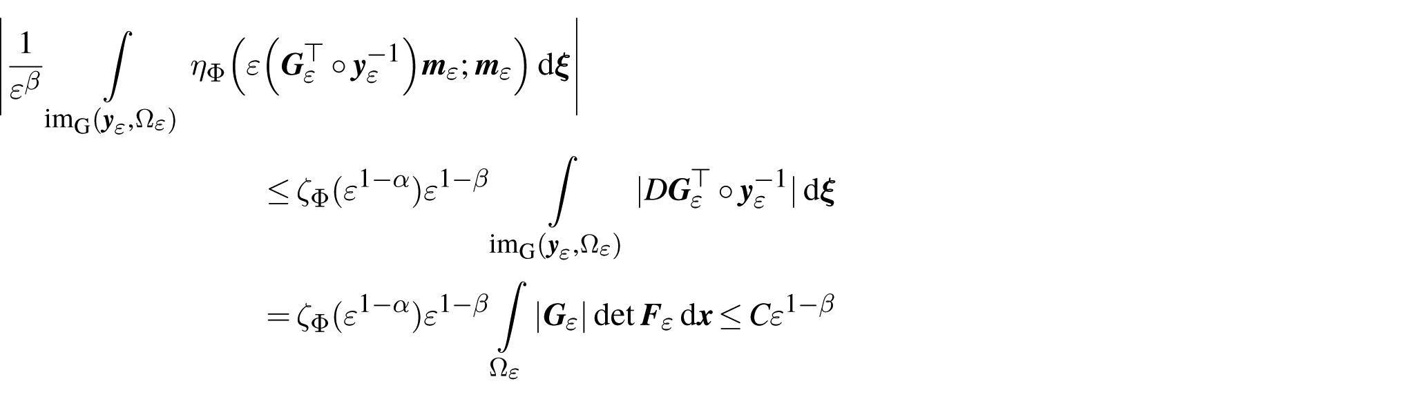
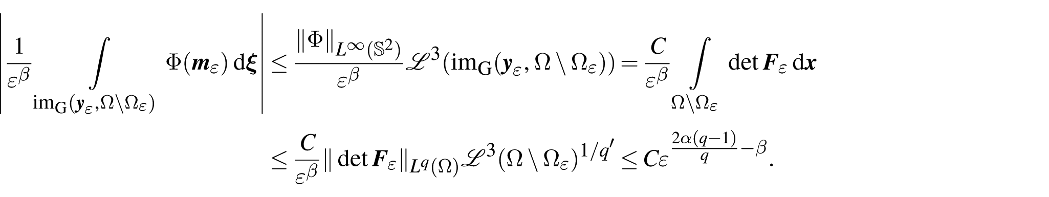
For the last two integrals on the right-hand side of (48), we observe that
and
thanks to the change-of-variable formula, (30), the boundedness of in , and (47). Thus, from (48), we deduce
Exploiting again Proposition 3.4, the integral on the right-hand side can be rewritten as
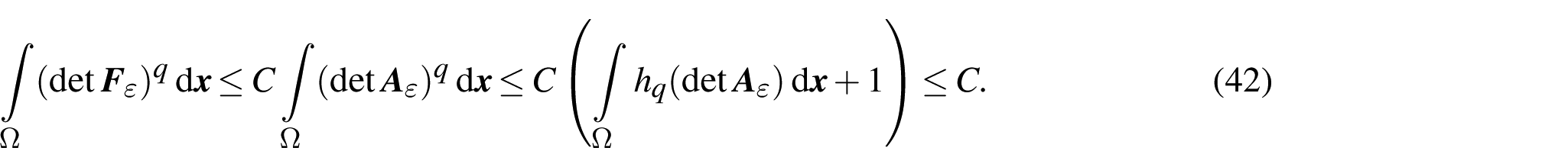
Using (42), (44), the change-of-variable formula, and Hölder’s inequality, the second term can be estimated as
Thus, from (49), we obtain
where
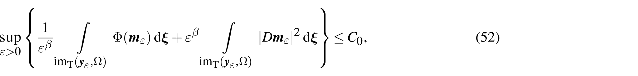
Noting that in view of (6) and (43), from (17) and (50) we obtain
where is a constant depending on the supremum in (17).
Given (18), by applying [11, Lemma 2.24 and Lemma 3.6(a)], we find a Lipschitz domain such that along a not relabeled subsequence. Hence, (52) yields
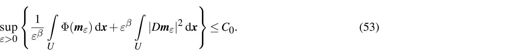
Let . Recall (31) and define . By [21, Lemma 4.2], we infer that with
From (53)–(54) and Young’s inequality, we find
while, trivially,
We deduce that the sequence is bounded in . Hence, there exists such that, up to subsequences,
as . Since the constant in (53) does not depend on U, by applying [11, Lemma 2.24 and Lemma 3.6(a)] with a sequence of Lipschitz domains invading Ω together with a diagonal argument, we realize that and we select a not relabeled subsequence for which (55) holds true for any domain .
Let and define by setting . We claim that
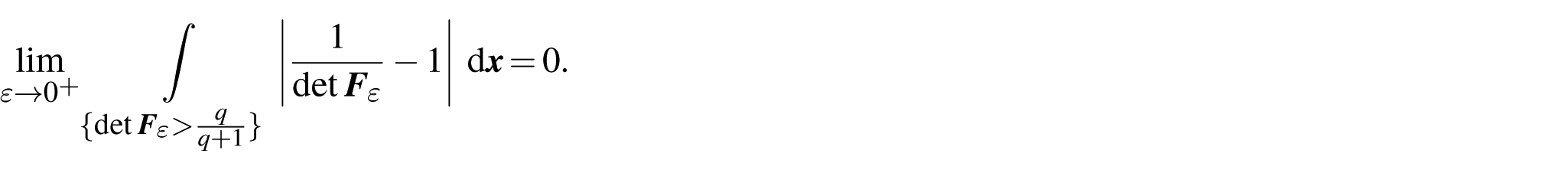
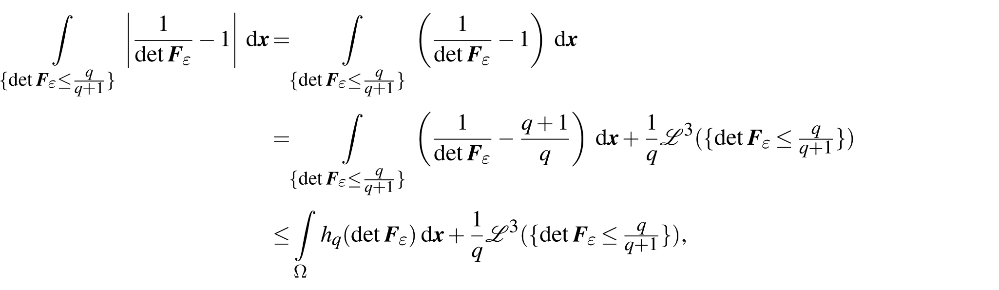
From (53), we have in . Hence, we can select a not relabeled subsequence with the property that, for almost every , there exists . Let and recall (31). For almost every , if , then but also , as , in view of (55). Thus, which entails . Therefore, for almost all and, by applying the dominated convergence theorem, we establish (56). Additionally, this argument ensures that for all as well as . Given the continuity of , by applying once again the dominated convergence theorem and comparing the result with (55), we realize that almost everywhere in Ω. Therefore, we deduce that each has finite perimeter in Ω and, in turn, . In particular, . Eventually, the combination of (39) and (56) easily gives (20).
Step 3 (Convergence of compositions). We move to the proof of (21). From (32) and the trivial inequality
we have
Then, thanks to (41), we find
By [44, Remark 3.5], we infer the equi-integrability of the sequence , while the same property trivially holds for . Therefore, given (18) and (20), the convergence in (21) is achieved by applying [14, Proposition 3.4] and the dominated convergence theorem. □
4.2. Gamma-convergence
Next, we move to the proof of the Γ-convergence result. We will consider the second-order Taylor expansion of W near the identity. Taking into account (W2)–(W5), we have
where , as . In particular, by (W3)–(W5), W has a global minimum at the identity, so that is a positive-semidefinite quadratic form and, hence, convex. Additionally, in view of the minor symmetries of the elasticity tensor [45, p. 195], and for all . Therefore, we have
For , we define
so that assumption (W2) yields
We begin by proving the lower bound.
Proof of claim (i) of Theorem 2.2. For convenience, the proof is split into two steps.
Step 1 (Lower bound for the elastic energy). As in the proof of Theorem 2.1, we set , , and . Additionally, we let . Given (11), we have
where
Similar to (33), we note that
As in Step 2 of the proof of Theorem 2.1, define for satisfying (43). From (19), we recover (44). Thus, in measure and, from (19) and (21), we infer
For convenience, let . From (33) and (60), we easily obtain
where the right-hand side goes to zero because of (43). Using the Taylor expansion (57), we write
For the first integral on the right-hand side, owing to the convexity of and (58), we have
thanks to (61)–(63). For the second one, we estimate
thanks to the boundedness of in coming from (19), and to (33) and (63). Hence, recalling (43), we obtain
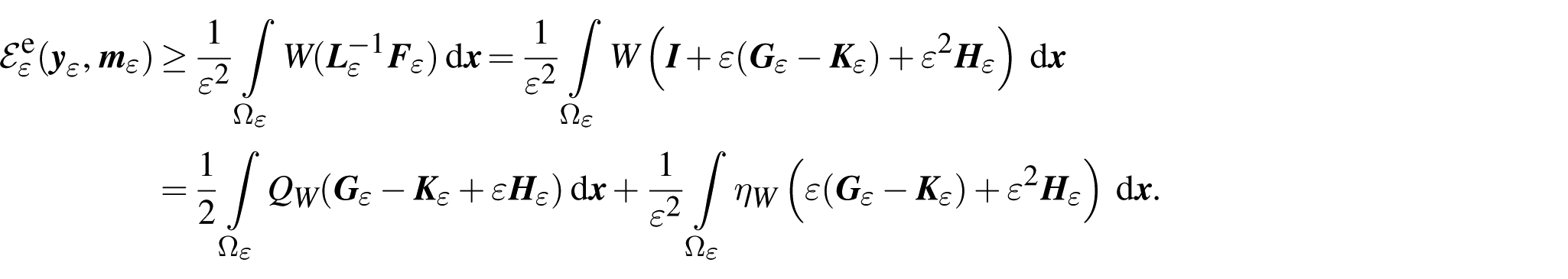
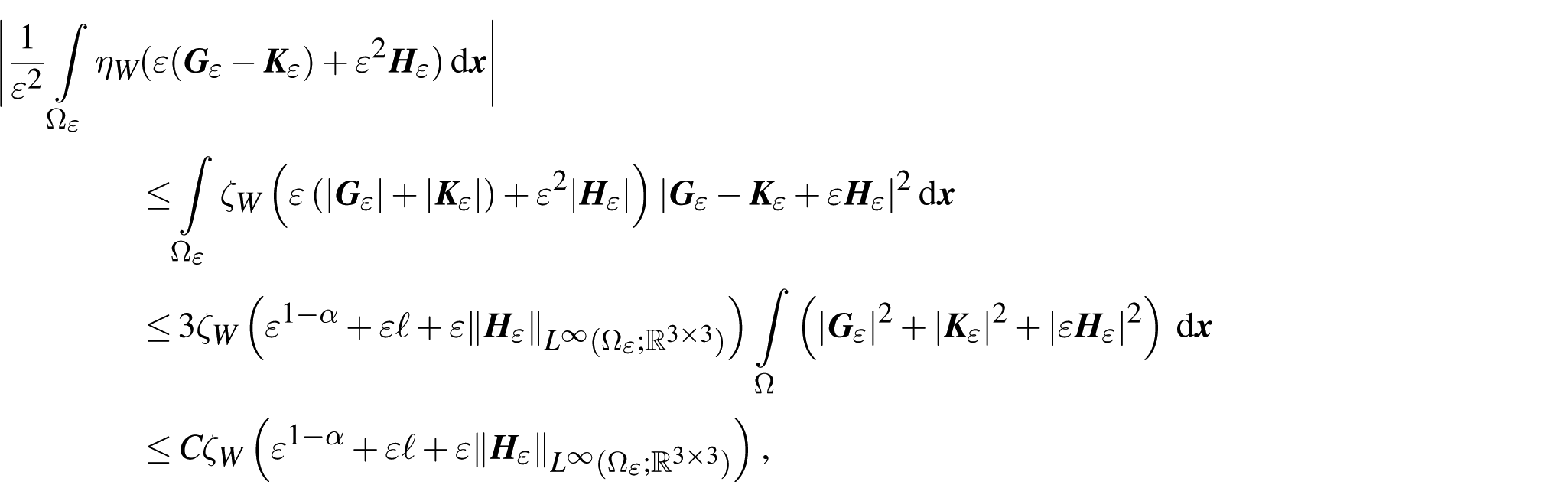
Step 2 (Lower bound for the magnetic energy). Without loss of generality, we assume (17) and we select a not relabeled subsequence for which the inferior limit of is attained as a limit.
By arguing as in Step 1 of the proof of Theorem 2.1, we conclude that the sequence is equi-integrable. Additionally, we recover (50) with defined as in (51) for some and, in turn,
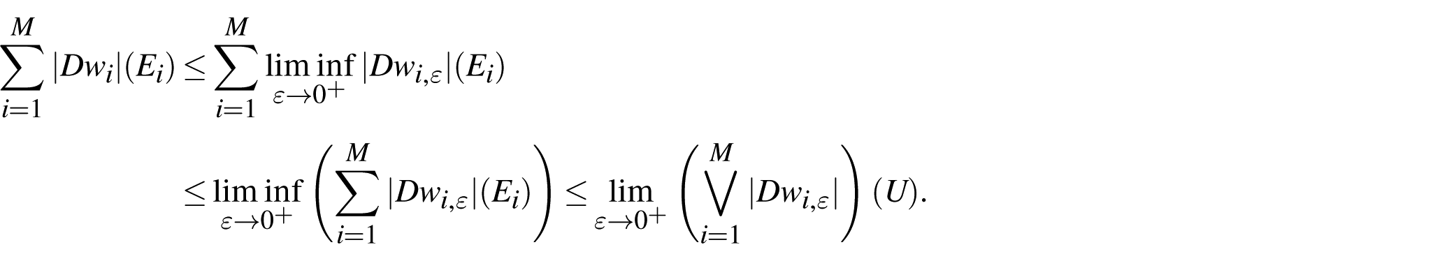
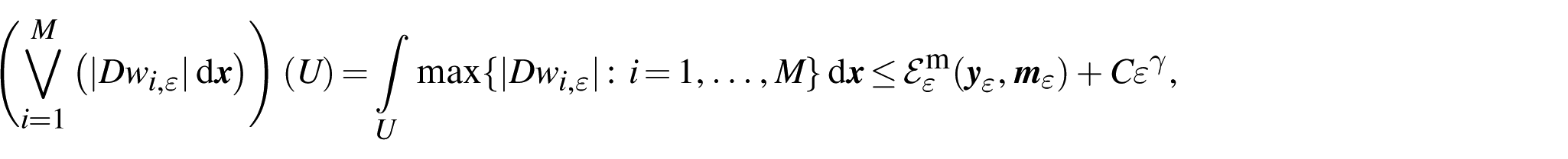
Let be arbitrary. Given (18), by [11, Lemma 2.24 and Lemma 3.6(a)], we deduce that for a not relabeled subsequence. Hence, (20) yields (56). Recalling (31), again by [30, Lemma 4.2] we have that satisfies (54) for all . Using (65) and Young’s inequality, we obtain
for any measurable subset , and, in turn,
where the equality is justified by (28). From (56), we obtain (55) for , where we employ (31). Therefore, taking the inferior limit, as , in the previous inequality by means of Lemma 3.6, then the supremum among all domains , and applying [30, Proposition 2.2], we obtain
Eventually, the combination of (64) and (66) proves (22). □
Proof of claim (ii) of Theorem 2.2. We subdivide the proof into three steps.
Step 1 (Reduction to Lipschitz displacements). We argue that it is sufficient to prove the claim for Lipschitz displacements. Given our assumptions on Δ and d, in view of [31, Proposition A.2], there exists a sequence in such that
so that, by dominated convergence,
Hence, if we show that there exists a recovery sequence for each , then the claim for u can be established by means of a standard diagonal argument (see, e.g., [24, Remark 1.29]). Henceforth, to avoid cumbersome notation, we will simply assume that and we will always consider its Lipschitz representative.
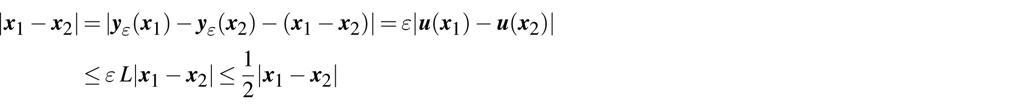
Step 2 (Construction of the recovery sequence). Setting , we consider . We define the Lipschitz map and we check that it is injective. Let with and, by contradiction, suppose that . Then
which provides a contradiction. A similar argument shows that the inverse deformation is also Lipschitz: given , we have
so that
since . This proves the claim and shows that
We observe that , , and . Also, (18) and (19) trivially hold.
Let . From [21, Theorem 2.6], we infer the existence of a sequence in satisfying
and
We set . To prove (20), fix . By the area formula,
while, for any , we have
thanks to the change-of-variable formula and the dominated convergence theorem with (18) and (67). Hence, in . As uniformly in Ω, the set is contained in any compact neighborhood of Ω, at least for , so that the previous convergence implies (20).
Step 3 (Attainment of the lower bound). First, we prove that
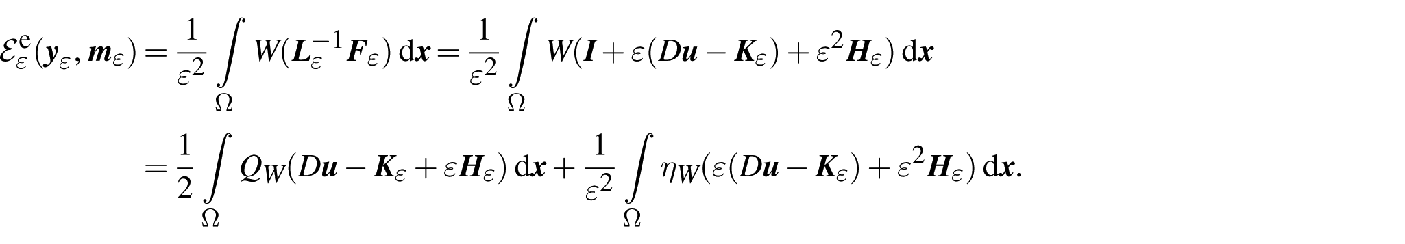
For convenience, noting that , we set , , and . Clearly, (67) yields
by the dominated convergence theorem. Similar to Step 1 in the proof of Theorem 2.2(i), we define
which still fulfills (60). Also, we let and, similar to (63), we check that
By considering the Taylor expansion (57), we write
Using (58), (70) and (71), and the dominated convergence theorem, we compute
As
in view of (33) and (71), then (69) follows thanks to (59).
Next, we prove that
Having (68) in mind, it is sufficient to check that
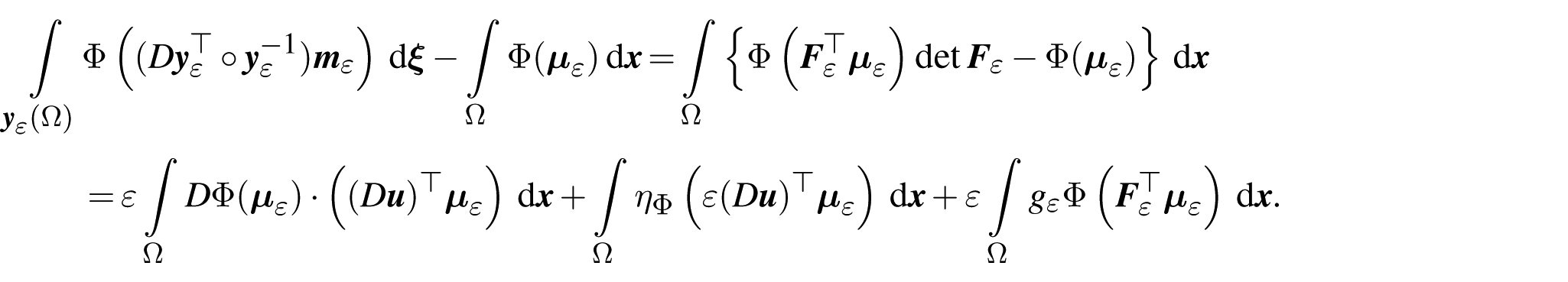
and
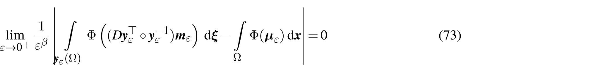
For (73), recalling (45)–(46), we observe that for a sequence bounded in . By applying the change-of-variable formula and considering the Taylor expansion of Φ in (29) around , we write
Thus, given a neighborhood V of , for we find
so that (73) follows from (6) and (30).
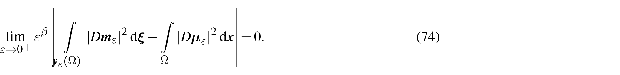
For (74), we observe that for a sequence bounded in . Indeed, using Neumann series,
where, for ,
Additionally, almost everywhere in thanks to the chain rule, and (68) entails
where we set . By applying the change-of-variable formula, we write
Therefore, (75) and the boundedness of the sequences and in and , respectively, yield
and, in turn, (74) follows.
This concludes the proof of (72) which, together with (69), gives (23). □
4.3. Convergence of almost minimizers
Before presenting the proof of Corollary 2.3, we discuss the well-posedness of the steady Maxwell system (24). More generally, given and , we consider the system
Solutions to the previous system will be considered in the distributional sense. Below, we refer to the homogeneous Sobolev space (sometimes named after Beppo Levi or Deny-Lions [46]) defined as
Proposition 4.1 (Well-posedness of the Maxwell system). Letwith. Then, there exists a unique distributional solutionto (76). Moreover, the solution operatoris linear and bounded on.
Proof. In view of the first equation, we can write for some . Hence, the system (76) is equivalent to the single equation
By [47, Theorem 5.1], the latter admits a unique distributional solution up to additive constants. The same result shows that the map defines a bounded linear operator on . □
For the proof of Corollary 2.3, we need the following result.
Proposition 4.2 (Additional compactness). Under the same assumptions of Theorem 2.1, we additionally have
Proof. First, we prove (77). For convenience, let again and . By (W5), we have
so that in . Recalling that by (40), we estimate
where the right-hand side goes to zero as . Thus,
As in Step 1 of Theorem 2.1, we have (38) and, from the convergence in measure, we obtain
Using (38) and dominated convergence, we easily see that
Then,
where the right-hand side goes to zero in view of (79) and (80). Therefore, (77) follows.
Next, we look at (78). For convenience, we write . By applying the change-of-variable formula, we compute
Given (77), letting in the previous equation yields
Let . By employing once again the change-of-variable formula, with the aid of the dominated convergence theorem, using (18) and (20)–(21), we obtain
Thus, in which, together with (81), gives (78). □
With Proposition 4.2 at hand, the result for almost minimizers follows from Theorem 2.1 and Theorem 2.2 in a standard manner.
Proof of Corollary 2.3. We consider a sequence with for all such that
By applying Theorem 2.2(ii) for limit with constantly equal to , we see that such sequences exist. From Proposition 4.2 to , we infer that the sequence with is bounded in . Thus,
in view of Proposition 4.1. Using Hölder’s inequality, we immediately find
Hence,
so that (25) entails
From this, we easily get
By applying Theorem 2.1 and Proposition 4.2 to the sequence , we identify for which (18)–(21) and (77)–(78) hold true. Proposition 4.1 ensures that and are well-defined and belong to . In particular, linearity and boundedness of the solution operator of the Maxwell system yield the estimate
and, in turn,
thanks to (78). Having in mind (20), we obtain
At this point, the minimality of and (26) follow from Theorem 2.2 by standard Γ-convergence arguments (see, e.g., [24, Remark 1.7]). □
4.4. Regularity of the limiting problem
Recalling that for we have (27), our problem is related to the regularity of perimeter minimizers. Specifically, we will refer to the notion of sets of almost minimal boundary [35].
Definition 4.3 (Set of almost minimal boundary). Let. A sethas ϰ-almost minimal boundary in Ω if, for every set, there existsuch that, for every, , andwith, there holds
In view of [35, Theorem 1], we known that is a surface of class whenever E has ϰ-almost minimal boundary in Ω.
We now present the proof of the regularity result. For convenience, we fix .
Proof of Theorem 2.4. We subdivide the proof into three steps.
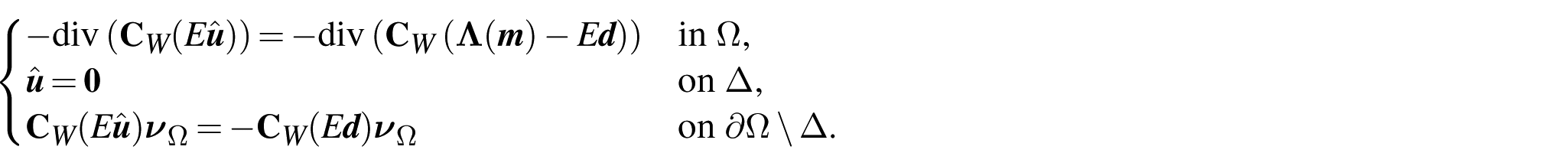
Step 1 (Regularity of the displacement). Let with on Δ. Testing the minimality of by taking as a competitor, we realize that u is a minimizer of . Thus, , where is the unique weak solution of the boundary value problem
Here, and denote the elasticity tensor of W and the outer unit normal to Ω, respectively. Note that . Therefore, standard elliptic regularity theory (see, e.g., [48, Theorem 16.4]) yields and, in turn, for all .
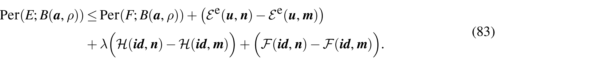
Step 2 (Regularity of the jump set). Let and . We claim that E is a set of ϰ-almost minimal boundary in Ω. To see this, we consider and we set . Let , , and with . We need to show that
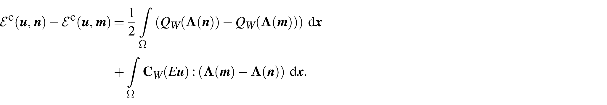
for some constant to be determined. Define by setting in F and in . Then, in . By minimality, from which we obtain
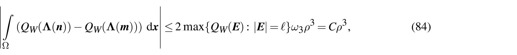
We estimate the three differences on the right-hand side of (83). We have
Recalling (33), the first summand on the right-hand side is easily estimated as
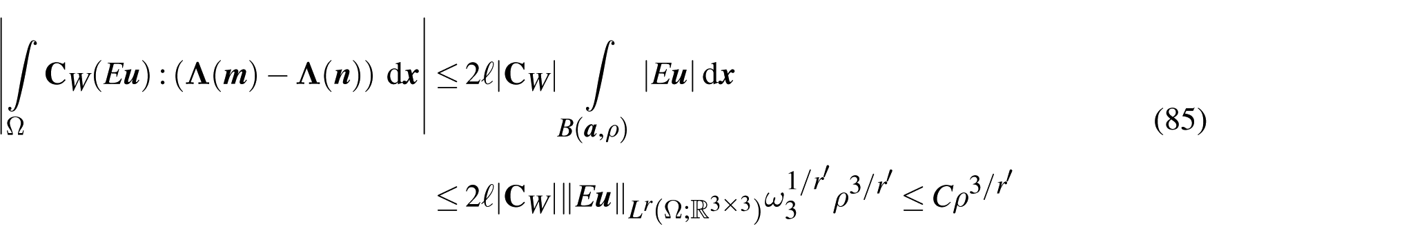
while for the second one we find
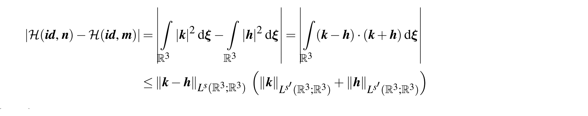
for any thanks to Hölder’s inequality. Writing and , the second difference on the right-hand side of (83) is bounded by
for any . Then, from Proposition 4.1, we infer the estimates
and
Thus,
Eventually, for the last difference on the right-hand side of (83), we have
Altogether, (83)–(87) yield the estimate
In particular, choosing and , by noting that , we obtain the desired estimate (82) with . Therefore, E is a set of ϰ-almost minimal boundary in Ω, so that is a surface of class in Ω.
Step 3 (Improved regularity for the displacement). Observe that is a closed subset of Ω. Let U be one of the connected components of . As m is constant on U, the displacement is a weak solution to the equation
Hence, if with , elliptic regularity theory (see, e.g., [48, Remark 15.16]) yields and, by Morrey’s embedding, . As the connected component U is arbitrary, we conclude . □
Footnotes
ORCID iD
Marco Bresciani
Funding
M.B. acknowledges the support of the Alexander von Humboldt Foundation. He is member of GNAMPA (Gruppo Nazionale per l’Analisi Matematica, la Probabilitá e le loro Applicazioni) of INdAM (Istituto Nazionale di Alta Matematica). The work of M.F. was supported by the DAAD (Deutscher Akademischer Austauschdienst) project 57702972.
Declaration of conflicting interests
The authors declared no potential conflicts of interest with respect to the research, authorship, and/or publication of this article.
References
1.
ApicellaVClementeCSDavinoD, et al. Review of modeling and control of magnetostrictive actuators. Actuators2019; 8: 45.
2.
GrimesCARoySCRaniS, et al. Theory, instrumentation and applications of magnetoelastic resonance sensors: a review. Sensors2011; 11: 2809–2844.
LandauLDLifshitzEM. Electrodynamics of continuous media, Course of Theoretical Physics, vol. 8. Pergamon Press, 1984.
7.
De SimoneAPodio-GuidugliP. On the continuum theory of deformable ferromagnetic solids. Arch Ration Mech Anal1996; 136: 201–233.
8.
JamesRDKinderlehrerD. Theory of magnetostriction with applications to TbxDy1−xFe2. Philos Mag B1993; 68: 237–274.
9.
KinderlehrerD. Magnetoelastic interactions. In: SerapioniRTomarelliF (eds) Variational methods for discontinuous structures, Progress in Nonlinear Differential Equations and Their Applications, vol. 25. Basel: Birkhauser, 1996.
10.
EricksenJL. On the Cauchy–Born rule. Math Mech Solids2008; 13(3–4): 199–220.
11.
BarchiesiMHenaoDMora-CorralC. Local invertibility in Sobolev spaces with applications to nematic elastomers and magnetoelasticity. Arch Ration Mech Anal2017; 224(2): 743–816.
12.
BrescianiM. Quasistatic evolutions in magnetoelasticity under subcritical coercivity assumptions. Calc Var Partial Differ Equ2023; 62: 181.
13.
BrescianiMDavoliEKružíkM. Existence results in large-strain magnetoelasticity. Ann Inst Henri Poincare Anal Non Lineaire2023; 40(3): 557–592.
14.
BrescianiMFriedrichMMora-CorralM. Variational models with Eulerian–Lagrangian formulation allowing for material failure. Arch Ration Mech Anal2025; 249: 4.
15.
KružíkMStefanelliUZemanJ. Existence results for incompressible magnetoelasticity. Discrete Contin Dyn Syst2015; 35: 5999–6013.
16.
BarchiesiMDe SimoneA. Frank energy for nematic elastomers: a nonlinear model. ESAIM Control Optim Calc Var2015; 21(2): 372–377.
17.
BrescianiMStroffoliniB. Quasistatic evolution of Orlicz–Sobolev nematic elastomers. Ann Mat Pura Appl2025; 204(6): 2489–2542.
18.
HenaoDStroffoliniB. On Sobolev–Orlicz nematic elastomers. Nonlinear Anal2020; 194: 111513.
19.
AlmiSKružíkMMolchanovaA. Linearization in magnetoelasticity. Adv Calc Var2025; 18(2): 577–591.
20.
JamesRDDe SimoneA. A constrained theory of magnetoelasticity. J Mech Phys Solids2002; 50(2): 283–320.
21.
AnzellottiGBaldoSVisintinA. Asymptotic behavior of the Landau–Lifschitz model of ferromagnetism. Appl Math Optim1991; 23(1): 171–192.
22.
GrandiDKružíkMMaininiE, et al. A phase-field approach to Eulerian interfacial energies. Arch Ration Mech Anal2019; 234: 351–373.
23.
GrandiDKružíkMMaininiE, et al. Equilibrium of multiphase solids with Eulerian interfaces. J Elast2020; 142: 409–431.
24.
BraidesA. Γ-convergence for beginners, Oxford Lecture Series in Mathematics and its Applications, vol. 22. Oxford: Oxford University Press, 2002.
25.
Dal MasoG. An introduction to Γ-convergence, Progress in Nonlinear Differential Equations and their Applications, vol. 8. Birkhauser, 1993.
26.
BrescianiM. Linearized von Kármán theory for incompressible magnetoelastic plates. Math Models Methods Appl Sci2021; 31(10): 1987–2037.
27.
BrescianiMKružíkM. A reduced model for plates arising as low energy Γ-limit in nonlinear magnetoelasticity. SIAM J Appl Math2023; 55(4): 3108–3168.
28.
Mora-CorralCOlivaM. Relaxation of nonlinear elastic energies involving the deformed configuration and applications to nematic elastomers. ESAIM Control Optim Calc Var2019; 25: 19.
29.
ScillaGStroffoliniB. Relaxation of nonlinear elastic energies related to Orlicz–Sobolev nematic elastomers. Rend Lincei Mat Appl2020; 31: 349–389.
30.
BaldoS. Minimal interface criterion for phase transitions in mixtures of Cahn–Hilliard fluids. Anal Inst Henri Poincare Anal Non Lineaire1990; 7(2): 67–90.
31.
AgostinianiVDal MasoGDe SimoneA. Linear elasticity obtained from finite elasticity by Γ-convergence under weak coerciveness conditions. Ann Inst H Poincare Anal Non Lineaire2021; 29: 715–735.
32.
MüllerS. Weak continuity of determinants and nonlinear elasticity. C R Acad Sci Paris Ser I Math1988; 307(9): 501–506.
33.
BallJM. Discontinuous equilibrium solutions and cavitation in nonlinear elasticity. Philos Trans Roy Soc London A1982; 306: 557–611.
34.
BallJM. Global invertibility of Sobolev functions and the interpenetration of matter. Proc Roy Soc Edinburgh A1981; 88: 315–328.
35.
TamaniniI. Boundaries of Caccioppoli sets with Hölder-continuous normal vector. J Reine Angew Math1982; 334: 27–39.
36.
AmbrosioLFuscoNPallaraD. Functions of bounded variations and free discontinuity problems. Oxford Mathematical Monographs. Oxford: Oxford University Press, 2000.
37.
HenaoDMora-CorralC. Fracture surfaces and the regularity of inverses for BV deformations. Arch Ration Mech Anal2011; 201(2): 575–629.
38.
FonsecaIGangboW. Degree theory in analysis and applications, Oxford Lecture Series in Mathematics and its Applications, vol. 2. Oxford University Press, 1995.
39.
MüllerS. Det = det. A remark on the distributional determinant. C R Acad Sci Paris Ser I Math1990; 311(1): 13–17.
40.
HenaoDMora-CorralC. Invertibility and weak continuity of the determinant for the modelling of cavitation and fracture in nonlinear elasticity. Arch Ration Mech Anal2010; 197: 619–655.
41.
FrieseckeGJamesRDMüllerS. A theorem on geometric rigidity and the derivation of nonlinear plate theory from three-dimensional elasticity. Comm Pure Appl Math2002; 55: 1461–1506.
42.
ContiSSchweizerB. Rigidity and gamma convergence for solid–solid phase transitions with SO(2) invariance. Comm Pure Appl Math2006; 59(6): 830–868.
43.
Dal MasoGNegriMPercivaleD. Linearized elasticity as Γ-limit of finite elasticity. Set Valued Var Anal2002; 10: 165–183.
44.
BrescianiM. Anisotropic energies for the modeling of cavitation in nonlinear elasticity. Adv Calc Var2026; 19(1): 71–84.
45.
GurtinME. An introduction to continuum mechanics, Mathematics in Science and Engineering, vol. 158. Cambridge, MA: Academic Press, 1981.
46.
DenyJLionsJL. Les espaces du type de Beppo Levi. Ann Inst Fourier1954; 5: 305–370.
47.
PraetoriusD. Analysis of the operator Δ−1 div arising in magnetic models. Z Anal Anwend2004; 23(3): 589–605.
48.
AmbrosioLCarlottoAMassaccesiA. Lecture notes on elliptic partial differential equations. Pisa: Scuola Normale Superiore di Pisa, 2010.