Uniqueness results for operators with a p -Laplacian structure

Abstract

The goal of this note is to present different uniqueness results for problems associated with pseudo-monotone operators having the structure of the p-Laplace operator. The results are quite different when the equations at hand have a strictly monotone lower order term. The topic uses different test functions depending on the assumptions of the coefficients of the operators. Some of them are used in the references mentioned below but most of the time we simplify them and compare their strength. At the end of the note, we introduce some new type of such operators for which uniqueness can be proved roughly speaking the same way.

MSC2020-Mathematics Subject Classification: 35A16, 35J60, 35J66, 35J92.

1. Introduction and notation

We will denote by Ω a bounded open subset of ${\mathrm{ℝ}}^n$ , $n\ge 1$ . We would like to consider problems of the following type:

$$\{\begin{array}{c}\multicolumn{1}{c}{u\in W_0^{1,p}(\mathrm{\Omega }),}\\ \multicolumn{1}{c}{-\mathrm{\nabla }\cdot (a(x,u)|\mathrm{\nabla }u{|}^{p-2}\mathrm{\nabla }u)+b(x,u)=f\mathrm{in}\mathrm{\Omega }.}\end{array}$$

(1)

Here $a,b$ are Carathéodory functions, p is a real number such that $p>1$ , $f\in W^{-1,p^{\prime }}(\mathrm{\Omega })$ , $p^{\prime }=\frac{p}{p-1}$ is the conjugate of p. We refer to [1–3] for the definition of the spaces used in this paper. We will assume that for some positive constants $\lambda ,\mathrm{\Lambda }$

$$\lambda \le a(x,u)\le \mathrm{\Lambda }\mathrm{a.e.}x\in \mathrm{\Omega },\mathrm{\forall }u\in \mathrm{ℝ}.$$

(2)

For b we will assume that

$$u\to b(x,u)\mathrm{is}\mathrm{nondecreasing}$$

(3)

and defines a continuous mapping from $L^p(\mathrm{\Omega })$ into $L^{p^{\prime }}(\mathrm{\Omega })$ . An important case will be when this mapping is increasing, i.e., satisfies

$$(b(x,u)-b(x,v))(u-v)>0\mathrm{a.e.}x\in \mathrm{\Omega },\mathrm{\forall }u\ne v\in \mathrm{ℝ}.$$

(4)

As a canonical example for b, one could think to

$$b(x,u)=\beta (x)|u{|}^{(p-2)}u$$

where β denotes some nonnegative function.

Note that we will consider (1) under its weak form which is

$$\{\begin{array}{c}\multicolumn{1}{c}{u\in W_0^{1,p}(\mathrm{\Omega }),}\\ \multicolumn{1}{c}{{\int }_{\mathrm{\Omega }}a(x,u)|\mathrm{\nabla }u{|}^{p-2}\mathrm{\nabla }u\cdot \mathrm{\nabla }v+b(x,u)\mathrm{vdx}=⟨f,v⟩\mathrm{\forall }v\in W_0^{1,p}(\mathrm{\Omega }).}\end{array}$$

(5)

This model problem will help us to stress out the ideas and address more involved issues. Our goal is mainly to give simple proofs of results spread in the literature, not always in their strongest form (cf. [4–11]), and when several proofs are available to compare their strength.

The paper is divided as follows. In the next section, we address the case of operators with a lower order term strictly monotone. In section 3, this strict monotonicity is removed which surprisingly makes the problems more involved. Finally, in the last section, we use our knowledge acquired previously to extend our results to some other operators, some of them new, with structures close the p-Laplacian.

Let us first recall an important inequality when dealing with operators close to the p-Laplacian (see, for instance, [2] for a proof). For any $p>1$ , there exists a constant $c_p>0$ such that

$$c_p{(|\xi |+|\zeta |)}^{p-2}|\xi -\zeta {|}^2\le (|\xi {|}^{p-2}\xi -|\zeta {|}^{p-2}\zeta )\cdot (\xi -\zeta )\mathrm{\forall }\xi ,\zeta \in {\mathrm{ℝ}}^n.$$

(6)

Here, like in equation (5), the scalar product in ${\mathrm{ℝ}}^n$ is denoted by a dot.

2. The case with lower order term strictly monotone

The first uniqueness result that we can establish is the following.

Theorem 1. Suppose that $a,b$ are Carathéodory functions satisfying (2)–(4). In addition, suppose that $u\to a(x,u)$ is Hölder continuous of exponent $\frac{1}{2}$ , i.e., that for some constant A one has

$$|a(x,u)-a(x,v)|\le A|u-v{|}^{\frac{1}{2}}\mathrm{a.e.}x\in \mathrm{\Omega },\mathrm{\forall }u,v\in \mathrm{ℝ}.$$

(7)

Then, if $u_i$ are solutions to equation (5) corresponding, respectively, to $f=f_i$ , $i=1,2$ one has

$$f_1\le f_2\Rightarrow u_1\le u_2.$$

(8)

(Note that in particular problem (5) admits at most one solution. $f_1\le f_2$ stands for

$$⟨f_1,v⟩\le ⟨f_1,v⟩,$$

(9)

for all $v\in W_0^{1,p}(\mathrm{\Omega })$ , $v\ge 0$ ).

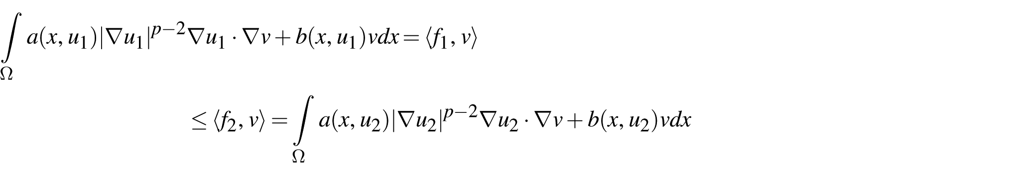
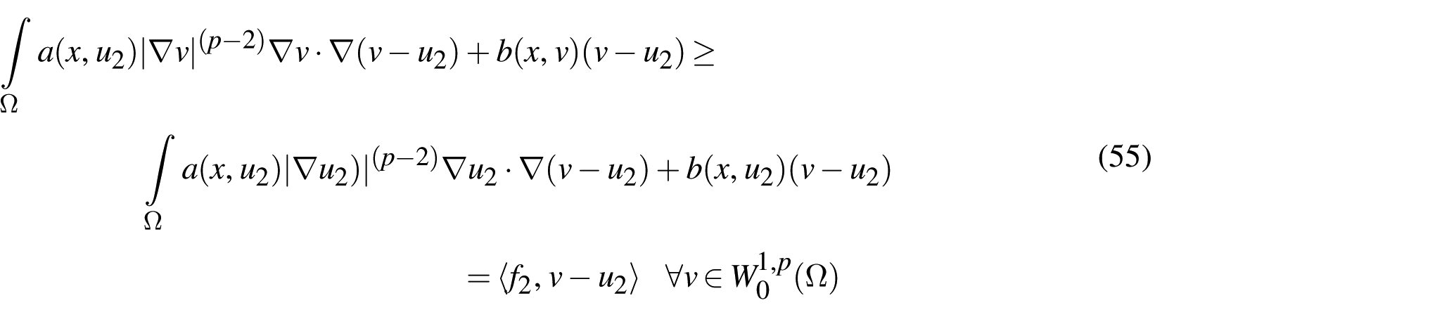
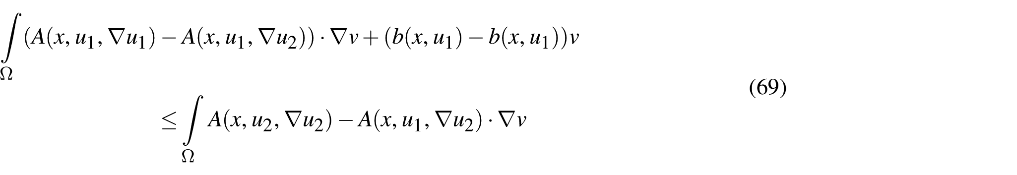
Proof. One has

$$\begin{array}{ccc}\multicolumn{1}{c}{\underset{\mathrm{\Omega }}{\mathrm{\int }}a(x,u_1)|\mathrm{\nabla }{u}_1{|}^{p-2}}& \multicolumn{1}{c}{\mathrm{\nabla }{u}_1\cdot \mathrm{\nabla }v+b(x,u_1)\mathrm{vdx}=⟨f_1,v⟩}& \multicolumn{1}{c}{}\\ \multicolumn{1}{c}{}& \multicolumn{1}{c}{\le ⟨f_2,v⟩=\underset{\mathrm{\Omega }}{\mathrm{\int }}a(x,u_2)|\mathrm{\nabla }{u}_2{|}^{p-2}\mathrm{\nabla }{u}_2\cdot \mathrm{\nabla }v+b(x,u_2)\mathrm{vdx}}\\ \multicolumn{1}{c}{}\end{array}$$

for all $v\in W_0^{1,p}(\mathrm{\Omega })$ , $v\ge 0$ .

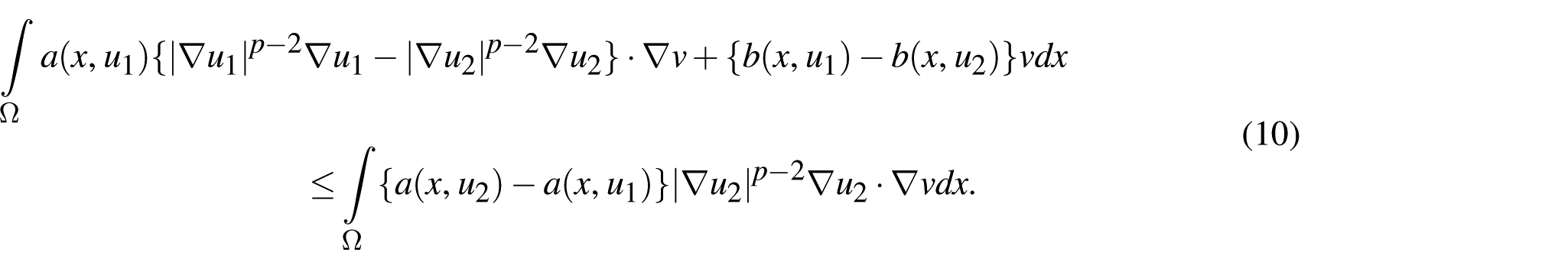
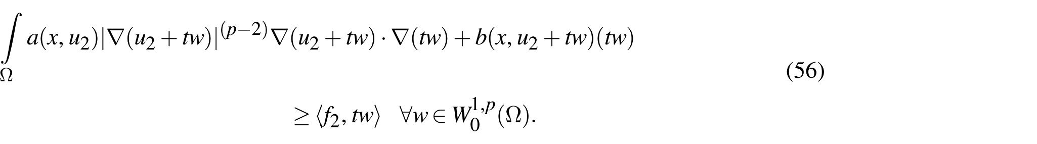
This implies easily subtracting ${\int }_{\mathrm{\Omega }}a(x,u_1)|\mathrm{\nabla }{u}_2{|}^{p-2}\mathrm{\nabla }{u}_2\cdot \mathrm{\nabla }\mathrm{vdx}$ to both sides of the inequality

$$\begin{array}{ccc}\multicolumn{1}{c}{\underset{\mathrm{\Omega }}{\mathrm{\int }}a(x,u_1)\{|\mathrm{\nabla }{u}_1{|}^{p-2}}& \multicolumn{1}{c}{\mathrm{\nabla }{u}_1-|\mathrm{\nabla }{u}_2{|}^{p-2}\mathrm{\nabla }{u}_2\}\cdot \mathrm{\nabla }v+\{b(x,u_1)-b(x,u_2)\}\mathrm{vdx}}& \multicolumn{1}{c}{}\\ \multicolumn{1}{c}{}& \multicolumn{1}{c}{\le \underset{\mathrm{\Omega }}{\mathrm{\int }}\{a(x,u_2)-a(x,u_1)\}|\mathrm{\nabla }{u}_2{|}^{p-2}\mathrm{\nabla }{u}_2\cdot \mathrm{\nabla }\mathrm{vdx}.}\\ \multicolumn{1}{c}{}\end{array}$$

(10)

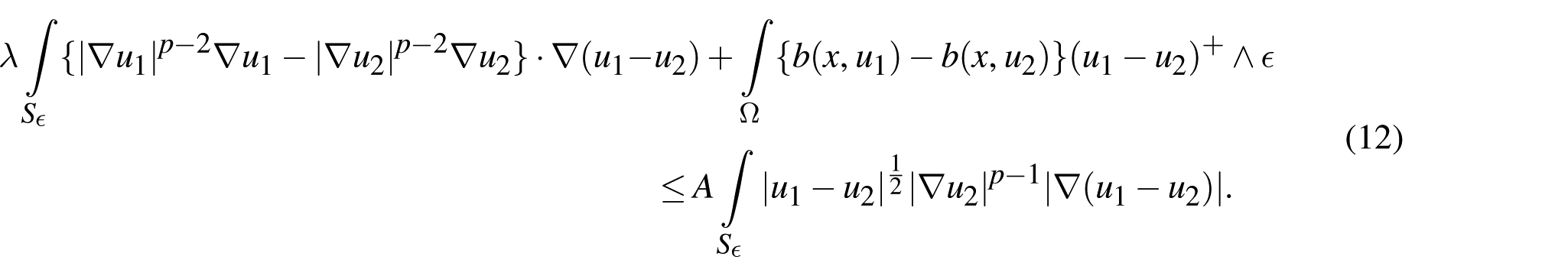
Then, for $ϵ>0$ one chooses as test function (cf. [6,12]) $v={(u_1-u_2)}^{+}\wedge ϵ$ where ∧ denotes the minimum of two numbers. One has

$$\mathrm{\nabla }v=\mathrm{\nabla }(u_1-u_2)\mathrm{on}{S}_{ϵ}=\{x\in \mathrm{\Omega }|0<(u_1-u_2)(x)<ϵ\},0\mathrm{else}.$$

(11)

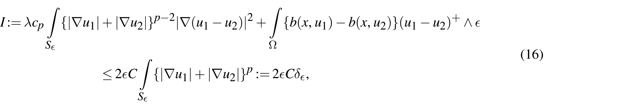
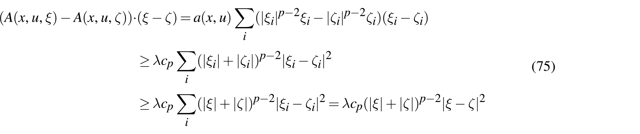
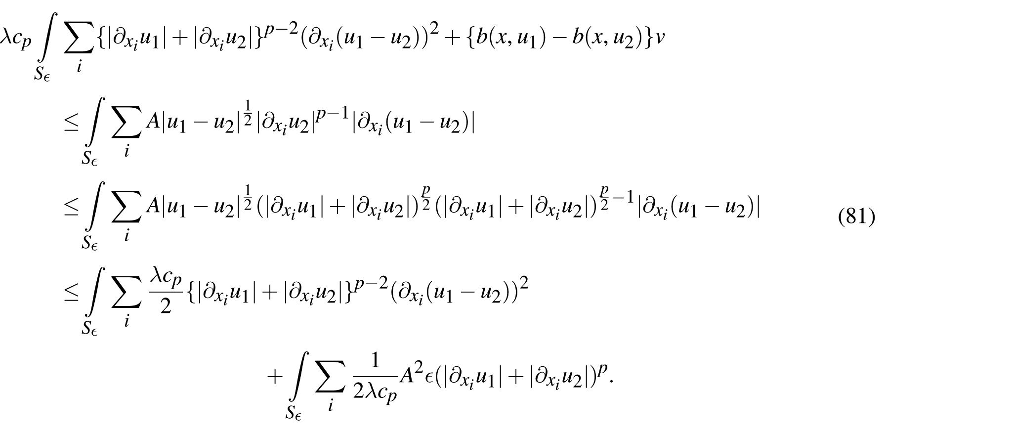
Taking into account (2), (7) one derives easily from equation (10) dropping the measures of integration

$$\begin{array}{ccc}\multicolumn{1}{c}{\lambda \underset{S_{ϵ}}{\mathrm{\int }}\{|\mathrm{\nabla }{u}_1{|}^{p-2}\mathrm{\nabla }{u}_1-|\mathrm{\nabla }{u}_2{|}^{p-2}\mathrm{\nabla }{u}_2\}\cdot \mathrm{\nabla }(u_1-}& \multicolumn{1}{c}{u_2)+\underset{\mathrm{\Omega }}{\mathrm{\int }}\{b(x,u_1)-b(x,u_2)\}{(u_1-u_2)}^{+}\wedge ϵ}& \multicolumn{1}{c}{}\\ \multicolumn{1}{c}{}& \multicolumn{1}{c}{\le A\underset{S_{ϵ}}{\mathrm{\int }}|u_1-u_2{|}^{\frac{1}{2}}|\mathrm{\nabla }{u}_2{|}^{p-1}|\mathrm{\nabla }(u_1-u_2)|.}\\ \multicolumn{1}{c}{}\end{array}$$

(12)

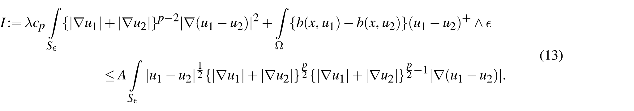
Using the inequality (6) this implies

$$\begin{array}{ccc}\multicolumn{1}{c}{I:=\lambda c_p\underset{S_{ϵ}}{\mathrm{\int }}\{|\mathrm{\nabla }{u}_1|}& \multicolumn{1}{c}{+|\mathrm{\nabla }{u}_2|{\}}^{p-2}|\mathrm{\nabla }(u_1-u_2){|}^2+\underset{\mathrm{\Omega }}{\mathrm{\int }}\{b(x,u_1)-b(x,u_2)\}{(u_1-u_2)}^{+}\wedge ϵ}& \multicolumn{1}{c}{}\\ \multicolumn{1}{c}{}& \multicolumn{1}{c}{\le A\underset{S_{ϵ}}{\mathrm{\int }}|u_1-u_2{|}^{\frac{1}{2}}{\{|\mathrm{\nabla }{u}_1|+|\mathrm{\nabla }{u}_2|\}}^{\frac{p}{2}}{\{|\mathrm{\nabla }{u}_1|+|\mathrm{\nabla }{u}_2|\}}^{\frac{p}{2}-1}|\mathrm{\nabla }(u_1-u_2)|.}\\ \multicolumn{1}{c}{}\end{array}$$

(13)

Applying the Young inequality

$$\mathrm{ab}\le \lambda c_p\frac{|a{|}^2}{2}+\frac{1}{\lambda c_p}\frac{|b{|}^2}{2}$$

(14)

in the right-hand side of the inequality we get for some constant $C=C(p,\lambda ,A)$

$$I:=\le \frac{\lambda c_p}{2}\underset{S_{ϵ}}{\mathrm{\int }}{\{|\mathrm{\nabla }{u}_1|+|\mathrm{\nabla }{u}_2|\}}^{p-2}|\mathrm{\nabla }(u_1-u_2){|}^2+C\underset{S_{ϵ}}{\mathrm{\int }}|u_1-u_2|{\{|\mathrm{\nabla }{u}_1|+|\mathrm{\nabla }{u}_2|\}}^p.$$

(15)

Thus, it comes

$$\begin{array}{ccc}\multicolumn{1}{c}{I:=\lambda c_p\underset{S_{ϵ}}{\mathrm{\int }}\{|\mathrm{\nabla }{u}_1|}& \multicolumn{1}{c}{+|\mathrm{\nabla }{u}_2|{\}}^{p-2}|\mathrm{\nabla }(u_1-u_2){|}^2+\underset{\mathrm{\Omega }}{\mathrm{\int }}\{b(x,u_1)-b(x,u_2)\}{(u_1-u_2)}^{+}\wedge ϵ}& \multicolumn{1}{c}{}\\ \multicolumn{1}{c}{}& \multicolumn{1}{c}{\le 2\mathrm{ϵC}\underset{S_{ϵ}}{\mathrm{\int }}{\{|\mathrm{\nabla }{u}_1|+|\mathrm{\nabla }{u}_2|\}}^p:=2\mathrm{ϵC}{\delta }_{ϵ},}\\ \multicolumn{1}{c}{}\end{array}$$

(16)

where, by the Lebesgue theorem, ${\delta }_{ϵ}\to 0$ when $ϵ\to 0$ . Then, one deduces that

$$\underset{\mathrm{\Omega }}{\mathrm{\int }}\{b(x,u_1)-b(x,u_2)\}\frac{{(u_1-u_2)}^{+}}{ϵ}\wedge 1\to 0$$

(17)

when $ϵ\to 0$ . Since $\frac{{(u_1-u_2)}^{+}}{ϵ}\wedge 1\to {\chi }_{\{u_1-u_2>0\}}$ a.e. where ${\chi }_{\{u_1-u_2>0\}}$ denotes the characteristic function of the set $\{u_1-u_2>0\}=\{x\in \mathrm{\Omega }|(u_1-u_2)(x)>0\}$ one deduces that

$$b(x,u_1)-b(x,u_2)=0\mathrm{a.e.}\mathrm{on}\{u_1-u_2>0\}.$$

(18)

If equation (4) holds, one has necessarily $u_1\le u_2$ . This completes the proof of the theorem. □

Remark 1. In case when $b(x,u)$ is not strictly monotone increasing one gets only that equation (18) holds.

It is clear from the above that the modulus of continuity of $u\to a(x,u)$ is playing a crucial role here. Working with this in mind one can produce a slightly better version than Theorem 2.1. Indeed, let us suppose that there is a continuous function ω such that

$$0<\omega (t)\mathrm{\forall }t>0,$$

(19)

$$|a(x,u)-a(x,v)|\le \omega (|u-v|)\mathrm{a.e.}x\in \mathrm{\Omega },\mathrm{\forall }u,v\in \mathrm{ℝ},$$

(20)

$$\underset{0^{+}}{\mathrm{\int }}\frac{\mathrm{dt}}{{\omega }^2(t)}=+\infty .$$

(21)

(ω could be the modulus of continuity of $u\to a(x,u)$ . Note that if a is Hölder continuous in u, i.e., if

$$|a(x,u)-a(x,v)|\le A|u-v{|}^{\beta }\mathrm{a.e.}x\in \mathrm{\Omega },\mathrm{\forall }u,v\in \mathrm{ℝ},$$

then $w(t)=A{t}^{\beta }$ satisfies the assumptions above when $\beta \ge \frac{1}{2}$ , thus our assumptions are slightly better than in Theorem 2.1.)

Then, we have

Theorem 2. Suppose that we are under the conditions of Theorem 1 and that equations (19)–(21) hold. Then, if $u_i$ are solutions to equation (5) corresponding, respectively, to $f=f_i$ , $i=1,2$ one has

$$f_1\le f_2\Rightarrow u_1\le u_2.$$

(22)

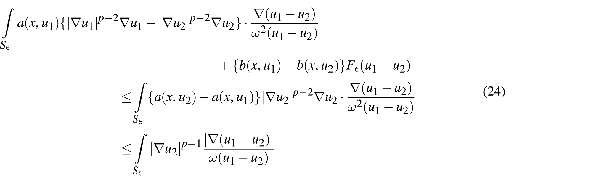
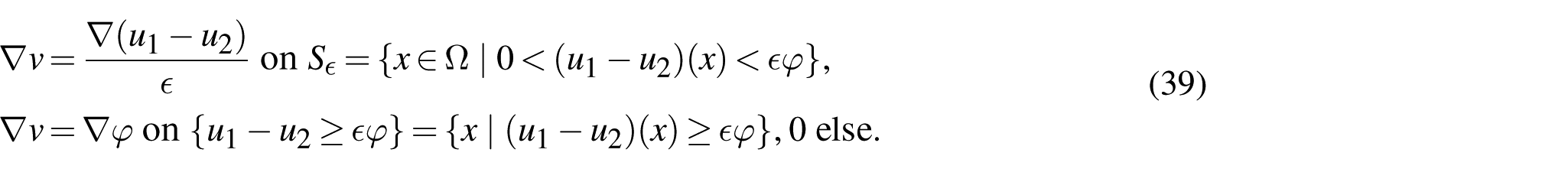
Proof. Since a is bounded (see equation (2)), there is no restriction in assuming ω bounded, replacing it if necessary by $\omega \wedge 2\mathrm{\Lambda }$ . Then, for $ϵ>0$ set

$$F_{ϵ}(x)=\{\begin{array}{c}\multicolumn{1}{c}{{\int }_{ϵ}^x\frac{\mathrm{dt}}{{\omega }^2(t)}\mathrm{for}x\ge ϵ,}\\ \multicolumn{1}{c}{0\mathrm{else.}}\end{array}$$

(23)

Clearly $F_{ϵ}$ is a piecewise $C^1$ -function with bounded derivative and

$$v=F_{ϵ}(u_1-u_2)$$

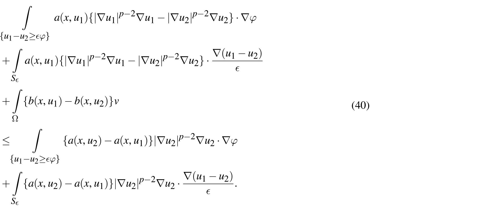
is a suitable test function for equation (10). Since

$$\mathrm{\nabla }{F}_{ϵ}(u_1-u_2)=\frac{\mathrm{\nabla }(u_1-u_2)}{{\omega }^2(u_1-u_2)}\mathrm{on}{S}_{ϵ}=\{x\in \mathrm{\Omega }|(u_1-u_2)(x)>ϵ\},0\mathrm{else},$$

one has arguing like in equation (10)

$$\begin{array}{ccc}\multicolumn{1}{c}{\underset{S_{ϵ}}{\mathrm{\int }}a(x,u_1)\{|\mathrm{\nabla }{u}_1{|}^{p-2}}& \multicolumn{1}{c}{\mathrm{\nabla }{u}_1-|\mathrm{\nabla }{u}_2{|}^{p-2}\mathrm{\nabla }{u}_2\}\cdot \frac{\mathrm{\nabla }(u_1-u_2)}{{\omega }^2(u_1-u_2)}}& \multicolumn{1}{c}{}\\ \multicolumn{1}{c}{}& \multicolumn{1}{c}{+\{b(x,u_1)-b(x,u_2)\}{F}_{ϵ}(u_1-u_2)}\\ \multicolumn{1}{c}{}& \multicolumn{1}{c}{\le \underset{S_{ϵ}}{\mathrm{\int }}\{a(x,u_2)-a(x,u_1)\}|\mathrm{\nabla }{u}_2{|}^{p-2}\mathrm{\nabla }{u}_2\cdot \frac{\mathrm{\nabla }(u_1-u_2)}{{\omega }^2(u_1-u_2)}}\\ \multicolumn{1}{c}{}& \multicolumn{1}{c}{\le \underset{S_{ϵ}}{\mathrm{\int }}|\mathrm{\nabla }{u}_2{|}^{p-1}\frac{|\mathrm{\nabla }(u_1-u_2)|}{\omega (u_1-u_2)}}\\ \multicolumn{1}{c}{}\end{array}$$

(24)

by equation (20). Using equations (2) and (6), we derive

$$\begin{array}{ccc}\multicolumn{1}{c}{I:=\lambda c_p\underset{S_{ϵ}}{\mathrm{\int }}\{|\mathrm{\nabla }{u}_1|+}& \multicolumn{1}{c}{|\mathrm{\nabla }{u}_2|{\}}^{p-2}\frac{|\mathrm{\nabla }(u_1-u_2){|}^2}{{\omega }^2(u_1-u_2)}+\{b(x,u_1)-b(x,u_2)\}{F}_{ϵ}(u_1-u_2)}& \multicolumn{1}{c}{}\\ \multicolumn{1}{c}{}& \multicolumn{1}{c}{\le \underset{S_{ϵ}}{\mathrm{\int }}{\{|\mathrm{\nabla }{u}_1|+|\mathrm{\nabla }{u}_2|\}}^{p-1}\frac{|\mathrm{\nabla }(u_1-u_2)|}{\omega (u_1-u_2)}}\\ \multicolumn{1}{c}{}& \multicolumn{1}{c}{=\underset{S_{ϵ}}{\mathrm{\int }}{\{|\mathrm{\nabla }{u}_1|+|\mathrm{\nabla }{u}_2|\}}^{\frac{p}{2}-1}\frac{|\mathrm{\nabla }(u_1-u_2)|}{\omega (u_1-u_2)}{\{|\mathrm{\nabla }{u}_1|+|\mathrm{\nabla }{u}_2|\}}^{\frac{p}{2}}.}\\ \multicolumn{1}{c}{}\end{array}$$

(25)

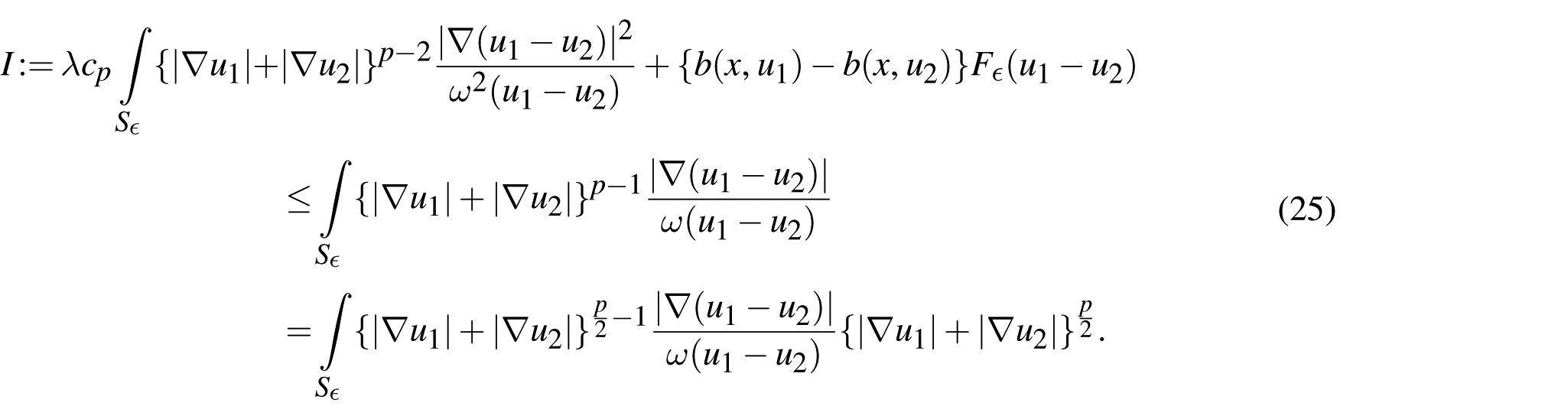
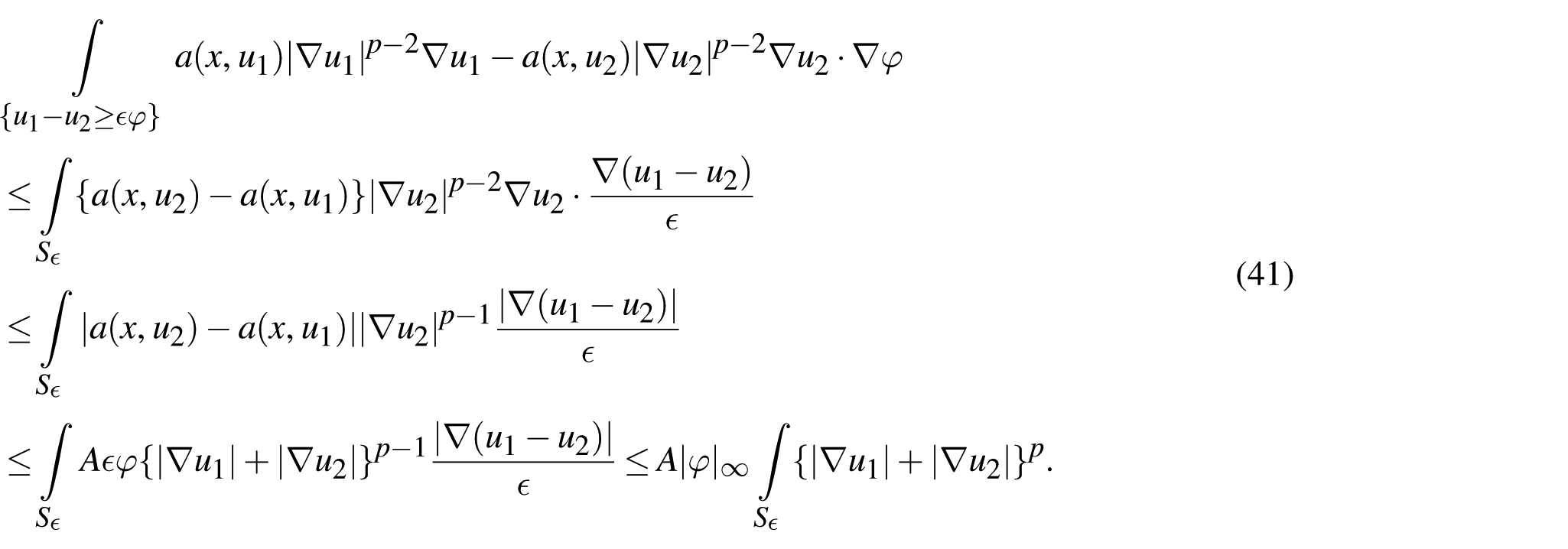
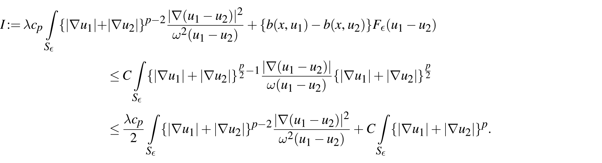
Using the Young inequality (14), we deduce like in equation (15)

$$I:=\le \frac{\lambda c_p}{2}\underset{S_{ϵ}}{\mathrm{\int }}{\{|\mathrm{\nabla }{u}_1|+|\mathrm{\nabla }{u}_2|\}}^{p-2}\frac{|\mathrm{\nabla }(u_1-u_2){|}^2}{{\omega }^2(u_1-u_2)}+C\underset{S_{ϵ}}{\mathrm{\int }}{\{|\mathrm{\nabla }{u}_1|+|\mathrm{\nabla }{u}_2|\}}^p,$$

(26)

and thus

$$\underset{\mathrm{\Omega }}{\mathrm{\int }}\{b(x,u_1)-b(x,u_2)\}{F}_{ϵ}(u_1-u_2)\le 2C\underset{S_{ϵ}}{\mathrm{\int }}{\{|\mathrm{\nabla }{u}_1|+|\mathrm{\nabla }{u}_2|\}}^p.$$

(27)

The left-hand side of equation (27) is bounded independently of ϵ and on the set $\{u_1-u_2>0\}$ one has $F_{ϵ}(u_1-u_2)\to +\infty$ . Due to equation (4), this implies that this set is of measure 0 and this completes the proof of the theorem. □

Remark 2. In the above theorems, the assumptions on the continuity of a are independent of p. Note that uniqueness might fail under just a continuity assumption of a in u (cf. [10]).

3. The case with no strict monotonicity of the lower order term

In this section, we address the case of a lower order term which is not strictly monotone or even vanishing identically. First, let us show

Theorem 3. Suppose that under the conditions of Theorem 2, $p\le 2$ and equations (19) and (20) hold with

$$\underset{0^{+}}{\mathrm{\int }}\frac{\mathrm{dt}}{\omega (t)}=+\infty .$$

(28)

Then, if $u_i$ are solutions to equation (5) corresponding, respectively, to $f=f_i$ , $i=1,2$ one has

$$f_1\le f_2\Rightarrow u_1\le u_2.$$

(29)

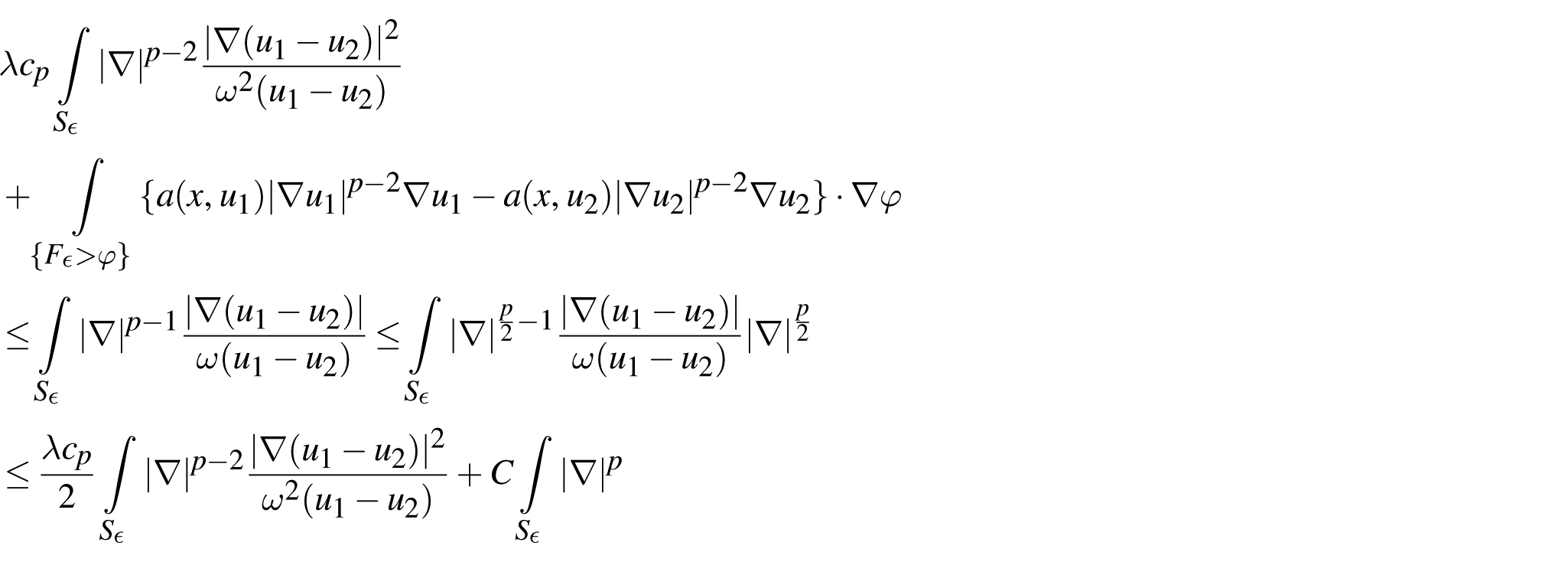
Proof. One proceeds as in Theorem 2. From equation (26), due to the monotonicity of $u\to b(x,u)$ , one deduces for some other constant C

$$\underset{S_{ϵ}}{\mathrm{\int }}{\{|\mathrm{\nabla }{u}_1|+|\mathrm{\nabla }{u}_2|\}}^{p-2}\frac{|\mathrm{\nabla }(u_1-u_2){|}^2}{{\omega }^2(u_1-u_2)}\le 2C\underset{S_{ϵ}}{\mathrm{\int }}{\{|\mathrm{\nabla }{u}_1|+|\mathrm{\nabla }{u}_2|\}}^p.$$

(30)

To simplify our notation, let us set

$$|\mathrm{\nabla }|=|\mathrm{\nabla }{u}_1|+|\mathrm{\nabla }{u}_2|.$$

(31)

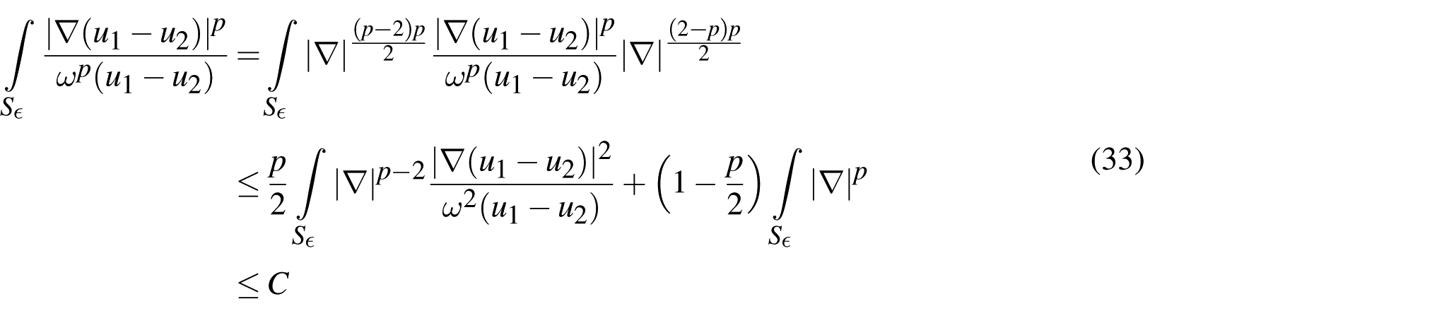
Then, by the Young inequality

$$\mathrm{ab}\le \frac{p}{2}|a{|}^{\frac{2}{p}}+(1-\frac{p}{2})|b{|}^{\frac{2}{2-p}}$$

(32)

we get

$$\begin{array}{ccc}\multicolumn{1}{c}{\underset{S_{ϵ}}{\mathrm{\int }}\frac{|\mathrm{\nabla }(u_1-u_2){|}^p}{{\omega }^p(u_1-u_2)}}& \multicolumn{1}{c}{=\underset{S_{ϵ}}{\mathrm{\int }}|\mathrm{\nabla }{|}^{\frac{(p-2)p}{2}}\frac{|\mathrm{\nabla }(u_1-u_2){|}^p}{{\omega }^p(u_1-u_2)}|\mathrm{\nabla }{|}^{\frac{(2-p)p}{2}}}& \multicolumn{1}{c}{}\\ \multicolumn{1}{c}{}& \multicolumn{1}{c}{\le \frac{p}{2}\underset{S_{ϵ}}{\mathrm{\int }}|\mathrm{\nabla }{|}^{p-2}\frac{|\mathrm{\nabla }(u_1-u_2){|}^2}{{\omega }^2(u_1-u_2)}+(1-\frac{p}{2})\underset{S_{ϵ}}{\mathrm{\int }}|\mathrm{\nabla }{|}^p}\\ \multicolumn{1}{c}{}& \multicolumn{1}{c}{\le C}\end{array}$$

(33)

for some constant C independent of ϵ (cf. equation (30)). Setting

$$G_{ϵ}(x)=\{\begin{array}{c}\multicolumn{1}{c}{{\int }_{ϵ}^x\frac{\mathrm{dt}}{\omega (t)}\mathrm{for}x\ge ϵ,}\\ \multicolumn{1}{c}{0\mathrm{else.}}\end{array}$$

(34)

one has due to Poincaré’s inequality

$$\underset{S_{ϵ}}{\mathrm{\int }}|G_{ϵ}(u_1-u_2){|}^p\le C_p\underset{S_{ϵ}}{\mathrm{\int }}|\mathrm{\nabla }{G}_{ϵ}(u_1-u_2){|}^p\le C_p\underset{S_{ϵ}}{\mathrm{\int }}\frac{|\mathrm{\nabla }(u_1-u_2){|}^p}{{\omega }^p(u_1-u_2)}$$

(35)

$C_p$ denoting the Poincaré constant. Combining this with equation (33), we get for some new constant C independent of ϵ

$$\underset{S_{ϵ}}{\mathrm{\int }}|G_{ϵ}(u_1-u_2){|}^p\le C.$$

Letting $ϵ\to 0$ since $G_{ϵ}(u_1-u_2)\to +\infty$ on the set $\{u_1-u_2>0\}$ we see that this set has measure 0. This completes the proof of the theorem. □

We can also show (see [6]):

Theorem 4. Suppose that equations (2) and (3) hold and in addition that

$$|a(x,u)-a(x,v)|\le A|u-v|\mathrm{a.e.}x\in \mathrm{\Omega },\mathrm{\forall }u,v\in \mathrm{ℝ}.$$

(36)

Let $u_i$ be solutions to equation (5) corresponding, respectively, to $f=f_i$ , $i=1,2$ . If $f_1\le f_2$ then

$$\underset{\{u_1-u_2>0\}}{\mathrm{\int }}a(x,u_1)|\mathrm{\nabla }{u}_1{|}^{(p-2)}\mathrm{\nabla }{u}_1\cdot \mathrm{\nabla }\phi =\underset{\{u_1-u_2>0\}}{\mathrm{\int }}a(x,u_2)|\mathrm{\nabla }{u}_2{|}^{(p-2)}\mathrm{\nabla }{u}_2\cdot \mathrm{\nabla }\phi$$

(37)

for all $\phi \in W^{1,p}(\mathrm{\Omega })\cap L^{\infty }(\mathrm{\Omega })$ , $\{u_1-u_2>0\}=\{x\in \mathrm{\Omega }|(u_1-u_2)(x)>0\}$ .

Proof. Suppose first that $\phi \in W^{1,p}(\mathrm{\Omega })\cap L^{\infty }(\mathrm{\Omega }),\phi \ge 0$ . Consider

$$v=\frac{{(u_1-u_2)}^{+}}{ϵ}\wedge \phi .$$

(38)

One has

$$\begin{array}{ccc}\multicolumn{1}{c}{}& \multicolumn{1}{c}{\mathrm{\nabla }v=\frac{\mathrm{\nabla }(u_1-u_2)}{ϵ}\mathrm{on}{S}_{ϵ}=\{x\in \mathrm{\Omega }|0<(u_1-u_2)(x)<\mathrm{ϵ\phi }\},}& \multicolumn{1}{c}{}\\ \multicolumn{1}{c}{}& \multicolumn{1}{c}{\mathrm{\nabla }v=\mathrm{\nabla }\phi \mathrm{on}\{u_1-u_2\ge \mathrm{ϵ\phi }\}=\{x|(u_1-u_2)(x)\ge \mathrm{ϵ\phi }\},0\mathrm{else}.}\end{array}$$

(39)

Thus, from equation (10), we derive

$$\begin{array}{ccc}\multicolumn{1}{c}{}& \multicolumn{1}{c}{\underset{\{u_1-u_2\ge \mathrm{ϵ\phi }\}}{\mathrm{\int }}a(x,u_1)\{|\mathrm{\nabla }{u}_1{|}^{p-2}\mathrm{\nabla }{u}_1-|\mathrm{\nabla }{u}_2{|}^{p-2}\mathrm{\nabla }{u}_2\}\cdot \mathrm{\nabla }\phi }& \multicolumn{1}{c}{}\\ \multicolumn{1}{c}{}& \multicolumn{1}{c}{+\underset{S_{ϵ}}{\mathrm{\int }}a(x,u_1)\{|\mathrm{\nabla }{u}_1{|}^{p-2}\mathrm{\nabla }{u}_1-|\mathrm{\nabla }{u}_2{|}^{p-2}\mathrm{\nabla }{u}_2\}\cdot \frac{\mathrm{\nabla }(u_1-u_2)}{ϵ}}\\ \multicolumn{1}{c}{}& \multicolumn{1}{c}{+\underset{\mathrm{\Omega }}{\mathrm{\int }}\{b(x,u_1)-b(x,u_2)\}v}\\ \multicolumn{1}{c}{}& \multicolumn{1}{c}{\le \underset{\{u_1-u_2\ge \mathrm{ϵ\phi }\}}{\mathrm{\int }}\{a(x,u_2)-a(x,u_1)\}|\mathrm{\nabla }{u}_2{|}^{p-2}\mathrm{\nabla }{u}_2\cdot \mathrm{\nabla }\phi }\\ \multicolumn{1}{c}{}& \multicolumn{1}{c}{+\underset{S_{ϵ}}{\mathrm{\int }}\{a(x,u_2)-a(x,u_1)\}|\mathrm{\nabla }{u}_2{|}^{p-2}\mathrm{\nabla }{u}_2\cdot \frac{\mathrm{\nabla }(u_1-u_2)}{ϵ}.}\\ \multicolumn{1}{c}{}\end{array}$$

(40)

Using the monotonicity of b (since one integrates on $u_1-u_2>0$ ) and equation (6), we are ending up with ( $|\phi {|}_{\infty }$ denotes the $L^{\infty }(\mathrm{\Omega })$ -norm of φ)

$$\begin{array}{ccc}\multicolumn{1}{c}{}& \multicolumn{1}{c}{\underset{\{u_1-u_2\ge \mathrm{ϵ\phi }\}}{\mathrm{\int }}a(x,u_1)|\mathrm{\nabla }{u}_1{|}^{p-2}\mathrm{\nabla }{u}_1-a(x,u_2)|\mathrm{\nabla }{u}_2{|}^{p-2}\mathrm{\nabla }{u}_2\cdot \mathrm{\nabla }\phi }& \multicolumn{1}{c}{}\\ \multicolumn{1}{c}{}& \multicolumn{1}{c}{\le \underset{S_{ϵ}}{\mathrm{\int }}\{a(x,u_2)-a(x,u_1)\}|\mathrm{\nabla }{u}_2{|}^{p-2}\mathrm{\nabla }{u}_2\cdot \frac{\mathrm{\nabla }(u_1-u_2)}{ϵ}}\\ \multicolumn{1}{c}{}& \multicolumn{1}{c}{\le \underset{S_{ϵ}}{\mathrm{\int }}|a(x,u_2)-a(x,u_1)\parallel \mathrm{\nabla }{u}_2{|}^{p-1}\frac{|\mathrm{\nabla }(u_1-u_2)|}{ϵ}}\\ \multicolumn{1}{c}{}& \multicolumn{1}{c}{\le \underset{S_{ϵ}}{\mathrm{\int }}\mathrm{Aϵ\phi }{\{|\mathrm{\nabla }{u}_1|+|\mathrm{\nabla }{u}_2|\}}^{p-1}\frac{|\mathrm{\nabla }(u_1-u_2)|}{ϵ}\le A|\phi {|}_{\infty }\underset{S_{ϵ}}{\mathrm{\int }}{\{|\mathrm{\nabla }{u}_1|+|\mathrm{\nabla }{u}_2|\}}^p.}\end{array}$$

(41)

Letting $ϵ\to 0$ it follows by the Lebesgue theorem that, when $\phi \ge 0$

$$\underset{\{u_1-u_2>0\}}{\mathrm{\int }}a(x,u_1)|\mathrm{\nabla }{u}_1{|}^{(p-2)}\mathrm{\nabla }{u}_1\cdot \mathrm{\nabla }\phi \le \underset{\{u_1-u_2>0\}}{\mathrm{\int }}a(x,u_2)|\mathrm{\nabla }{u}_2{|}^{(p-2)}\mathrm{\nabla }{u}_2\cdot \mathrm{\nabla }\phi .$$

(42)

Changing then φ into $\pm \phi +|\phi {|}_{\infty }$ , equation (37) follows. This completes the proof of the theorem. □

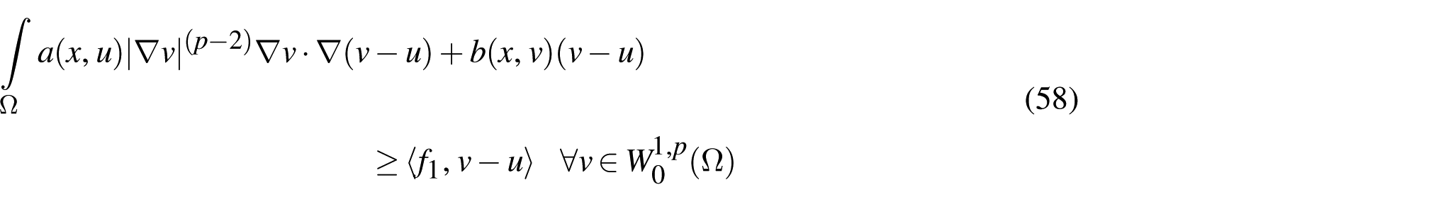
The assumption (36) can be improved. Indeed, one has as previously:

Theorem 5. Suppose that equations (2) and (3) hold and in addition that equations (19)–(21) hold. Let $u_i$ be solutions to equation (5) corresponding, respectively, to $f=f_i$ , $i=1,2$ . If $f_1\le f_2$ then equation (37) holds, i.e.,

$$\underset{\{u_1-u_2>0\}}{\mathrm{\int }}a(x,u_1)|\mathrm{\nabla }{u}_1{|}^{(p-2)}\mathrm{\nabla }{u}_1\cdot \mathrm{\nabla }\phi =\underset{\{u_1-u_2>0\}}{\mathrm{\int }}a(x,u_2)|\mathrm{\nabla }{u}_2{|}^{(p-2)}\mathrm{\nabla }{u}_2\cdot \mathrm{\nabla }\phi$$

for all $\phi \in W^{1,p}(\mathrm{\Omega })\cap L^{\infty }(\mathrm{\Omega })$ , $\{u_1-u_2>0\}=\{x\in \mathrm{\Omega }|(u_1-u_2)(x)>0\}$ .

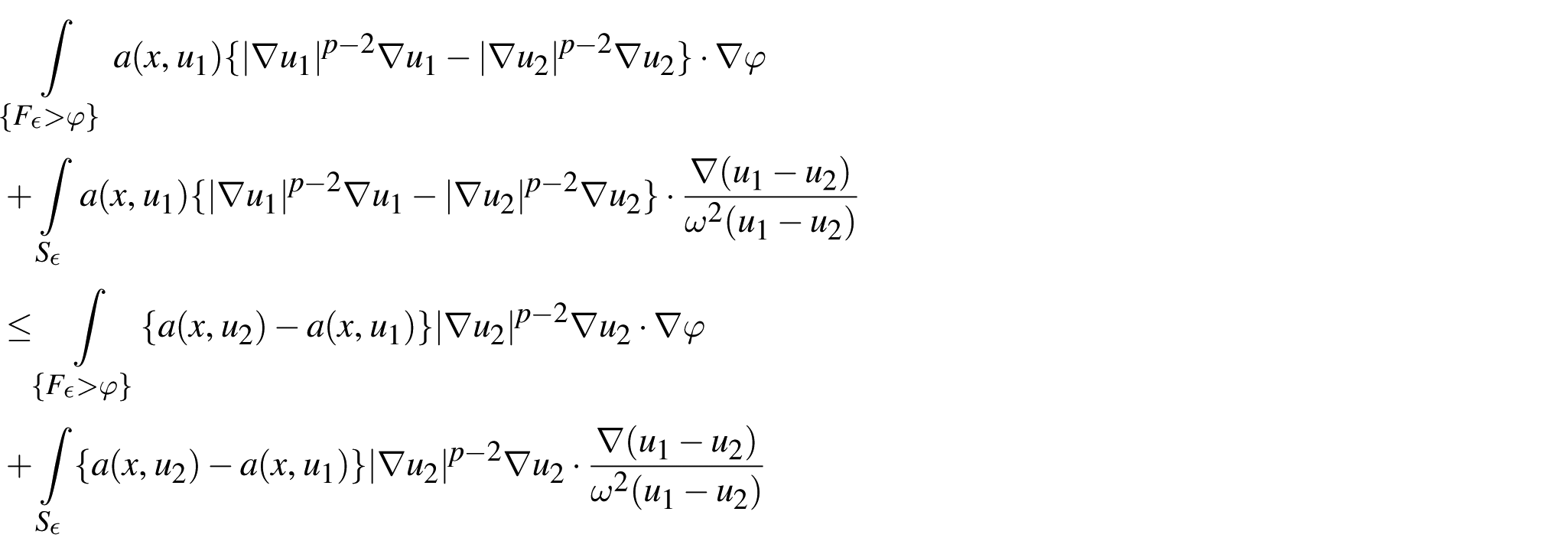
Proof. Let us suppose $F_{ϵ}$ defined as in equation (23). For $\phi \ge 0$ consider

$$v=F_{ϵ}(u_1-u_2)\wedge \phi$$

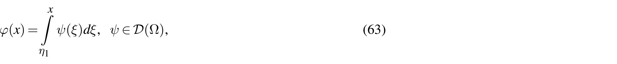
in equation (10). Since one integrates on $u_1-u_2\ge 0$ the term in b is nonnegative and one derives

$$\begin{array}{cc}\multicolumn{1}{c}{}& \multicolumn{1}{c}{\underset{\{F_{ϵ}>\phi \}}{\mathrm{\int }}a(x,u_1)\{|\mathrm{\nabla }{u}_1{|}^{p-2}\mathrm{\nabla }{u}_1-|\mathrm{\nabla }{u}_2{|}^{p-2}\mathrm{\nabla }{u}_2\}\cdot \mathrm{\nabla }\phi }\\ \multicolumn{1}{c}{}& \multicolumn{1}{c}{+\underset{S_{ϵ}}{\mathrm{\int }}a(x,u_1)\{|\mathrm{\nabla }{u}_1{|}^{p-2}\mathrm{\nabla }{u}_1-|\mathrm{\nabla }{u}_2{|}^{p-2}\mathrm{\nabla }{u}_2\}\cdot \frac{\mathrm{\nabla }(u_1-u_2)}{{\omega }^2(u_1-u_2)}}\\ \multicolumn{1}{c}{}& \multicolumn{1}{c}{\le \underset{\{F_{ϵ}>\phi \}}{\mathrm{\int }}\{a(x,u_2)-a(x,u_1)\}|\mathrm{\nabla }{u}_2{|}^{p-2}\mathrm{\nabla }{u}_2\cdot \mathrm{\nabla }\phi }\\ \multicolumn{1}{c}{}& \multicolumn{1}{c}{+\underset{S_{ϵ}}{\mathrm{\int }}\{a(x,u_2)-a(x,u_1)\}|\mathrm{\nabla }{u}_2{|}^{p-2}\mathrm{\nabla }{u}_2\cdot \frac{\mathrm{\nabla }(u_1-u_2)}{{\omega }^2(u_1-u_2)}}\end{array}$$

where

$$\begin{array}{c}\multicolumn{1}{c}{\{F_{ϵ}>\phi \}=\{x\in \mathrm{\Omega }|F_{ϵ}((u_1-u_2)(x))>\phi (x)\}}\\ \multicolumn{1}{c}{S_{ϵ}=\{x\in \mathrm{\Omega }|u_1-u_2(x)>ϵ,F_{ϵ}((u_1-u_2)(x))\le \phi (x)\}.}\end{array}$$

Using the same arguments as before one derives

$$\begin{array}{ccc}\multicolumn{1}{c}{}& \multicolumn{1}{c}{\lambda c_p\underset{S_{ϵ}}{\mathrm{\int }}|\mathrm{\nabla }{|}^{p-2}\frac{|\mathrm{\nabla }(u_1-u_2){|}^2}{{\omega }^2(u_1-u_2)}}& \multicolumn{1}{c}{}\\ \multicolumn{1}{c}{}& \multicolumn{1}{c}{+\underset{\{F_{ϵ}>\phi \}}{\mathrm{\int }}\{a(x,u_1)|\mathrm{\nabla }{u}_1{|}^{p-2}\mathrm{\nabla }{u}_1-a(x,u_2)|\mathrm{\nabla }{u}_2{|}^{p-2}\mathrm{\nabla }{u}_2\}\cdot \mathrm{\nabla }\phi }\\ \multicolumn{1}{c}{}& \multicolumn{1}{c}{\le \underset{S_{ϵ}}{\mathrm{\int }}|\mathrm{\nabla }{|}^{p-1}\frac{|\mathrm{\nabla }(u_1-u_2)|}{\omega (u_1-u_2)}\le \underset{S_{ϵ}}{\mathrm{\int }}|\mathrm{\nabla }{|}^{\frac{p}{2}-1}\frac{|\mathrm{\nabla }(u_1-u_2)|}{\omega (u_1-u_2)}|\mathrm{\nabla }{|}^{\frac{p}{2}}}\\ \multicolumn{1}{c}{}& \multicolumn{1}{c}{\le \frac{\lambda c_p}{2}\underset{S_{ϵ}}{\mathrm{\int }}|\mathrm{\nabla }{|}^{p-2}\frac{|\mathrm{\nabla }(u_1-u_2){|}^2}{{\omega }^2(u_1-u_2)}+C\underset{S_{ϵ}}{\mathrm{\int }}|\mathrm{\nabla }{|}^p}\end{array}$$

and then

$$\underset{\{F_{ϵ}>\phi \}}{\mathrm{\int }}\{a(x,u_1)|\mathrm{\nabla }{u}_1{|}^{p-2}\mathrm{\nabla }{u}_1-a(x,u_2)|\mathrm{\nabla }{u}_2{|}^{p-2}\mathrm{\nabla }{u}_2\}\cdot \mathrm{\nabla }\phi \le C\underset{S_{ϵ}}{\mathrm{\int }}|\mathrm{\nabla }{|}^p.$$

(43)

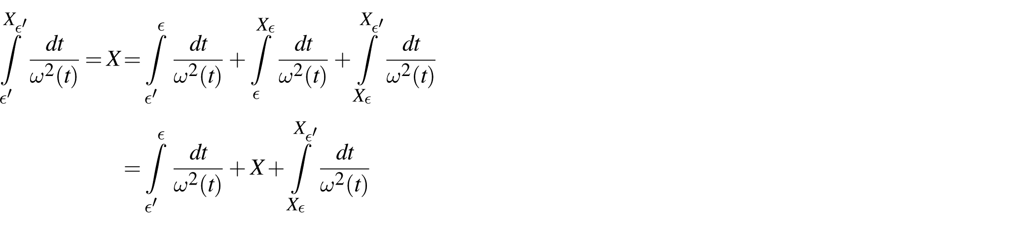
The function $F_{ϵ}(X)$ is increasing with $X>ϵ$ . For any $X>0$ one denotes by $X_{ϵ}$ the real number defined as

$$X_{ϵ}=F_{ϵ}^{-1}(X)\iff {\int }_{ϵ}^{X_{ϵ}}\frac{\mathrm{dt}}{{\omega }^2(t)}=X.$$

For ${ϵ}^{\prime }<ϵ$ one has $X_{{ϵ}^{\prime }}<X_{ϵ}$ . Indeed, this follows from

$$\begin{array}{ccc}\multicolumn{1}{c}{\underset{{ϵ}^{\prime }}{\overset{X_{{ϵ}^{\prime }}}{\mathrm{\int }}}\frac{\mathrm{dt}}{{\omega }^2(t)}=X}& \multicolumn{1}{c}{=\underset{{ϵ}^{\prime }}{\overset{ϵ}{\mathrm{\int }}}\frac{\mathrm{dt}}{{\omega }^2(t)}+\underset{ϵ}{\overset{X_{ϵ}}{\mathrm{\int }}}\frac{\mathrm{dt}}{{\omega }^2(t)}+\underset{X_{ϵ}}{\overset{X_{{ϵ}^{\prime }}}{\mathrm{\int }}}\frac{\mathrm{dt}}{{\omega }^2(t)}}& \multicolumn{1}{c}{}\\ \multicolumn{1}{c}{}& \multicolumn{1}{c}{=\underset{{ϵ}^{\prime }}{\overset{ϵ}{\mathrm{\int }}}\frac{\mathrm{dt}}{{\omega }^2(t)}+X+\underset{X_{ϵ}}{\overset{X_{{ϵ}^{\prime }}}{\mathrm{\int }}}\frac{\mathrm{dt}}{{\omega }^2(t)}}\\ \multicolumn{1}{c}{}\end{array}$$

since then

$$\underset{{ϵ}^{\prime }}{\overset{ϵ}{\mathrm{\int }}}\frac{\mathrm{dt}}{{\omega }^2(t)}+{\int }_{X_{ϵ}}^{X_{{ϵ}^{\prime }}}\frac{\mathrm{dt}}{{\omega }^2(t)}=0$$

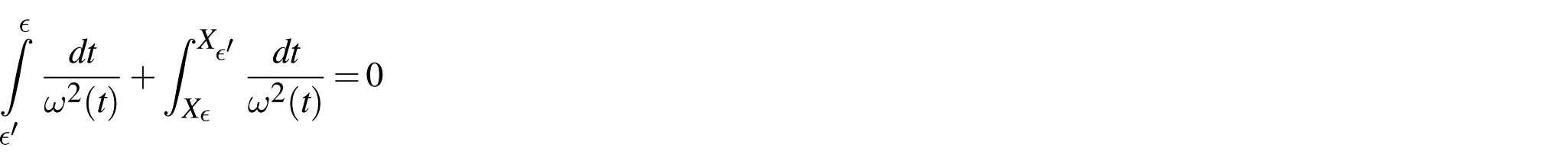
implies clearly $X_{{ϵ}^{\prime }}<X_{ϵ}$ . Then, when $ϵ\to 0$ , $X_{ϵ}$ has a limit which can only be 0 due to equation (21). Since

$$S_{ϵ}=\{x\in \mathrm{\Omega }|ϵ<(u_1-u_2)(x),(u_1-u_2)(x)\le F_{ϵ}^{-1}(\phi (x))\}.$$

the measure of $S_{ϵ}$ tends to 0 when $ϵ\to 0$ . One has also

$$\{F_{ϵ}>\phi \}=\{x\in \mathrm{\Omega }|(u_1-u_2)(x)>F_{ϵ}^{-1}(\phi (x))\vee ϵ\}$$

and thus

$${\chi }_{\{F_{ϵ}>\phi \}}\to {\chi }_{\{u_1-u_2>0\}}.$$

Passing to the limit in equations (43) and (37) is deduced as in the preceding theorem. This completes the proof of the theorem. □

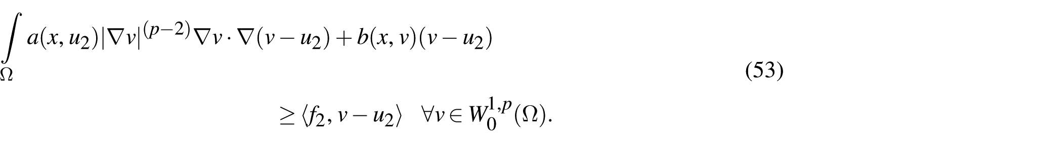
We are now going to draw consequences of equation (37). For that let us suppose that

$$\{u_1-u_2>0\}\mathrm{is}\mathrm{open}.$$

(44)

Then, by equation (37), one has on this set

$$f_1=-\mathrm{\nabla }\cdot \{a(x,u_1)|\mathrm{\nabla }{u}_1{|}^{(p-2)}\mathrm{\nabla }{u}_1\}=-\mathrm{\nabla }\cdot \{a(x,u_2)|\mathrm{\nabla }{u}_2{|}^{(p-2)}\mathrm{\nabla }{u}_2\}=f_2.$$

(45)

In particular, if $f_1$ is never equal to $f_2$ on this set, then it is empty, i.e., $u_1\le u_2$ . Consider, for instance,

$$f_1,f_2=f_1+ϵ.$$

(46)

Then, for any couple of solutions $u_1$ and $u_2=u_2(ϵ)$ , one has

$$u_1\le u_2(ϵ).$$

(47)

Similarly for any couple of solutions

$$u_1({ϵ}^{\prime }),u_2(ϵ),{ϵ}^{\prime }\le ϵ$$

(48)

one has

$$u_1({ϵ}^{\prime })\le u_2(ϵ).$$

(49)

Then, one has also

Proposition 3.1. Suppose $b(x,0)=0$ . Any solution $u_2(ϵ)$ converges toward a solution to

$$\underset{\mathrm{\Omega }}{\mathrm{\int }}a(x,u_1)|\mathrm{\nabla }{u}_1{|}^{(p-2)}\mathrm{\nabla }{u}_1\cdot \mathrm{\nabla }v+b(x,u_1)v=⟨f_1,v⟩\mathrm{\forall }v\in W_0^{1,p}(\mathrm{\Omega })$$

(50)

when $ϵ\to 0$ .

Proof. Taking $v=u_2$ in the definition of $u_2$ leads to

$$\underset{\mathrm{\Omega }}{\mathrm{\int }}a(x,u_2)|\mathrm{\nabla }{u}_2{|}^p\le ⟨f_1+ϵ,v⟩\le |f_1+ϵ{|}_{-1,p^{\prime }}||\mathrm{\nabla }{u}_2|{|}_p.$$

(51)

( $|{|}_p$ denotes the usual $L^p(\mathrm{\Omega })$ -norm). Hence, by equation (1)

$$\lambda ||\mathrm{\nabla }{u}_2|{|}_p^p\le C||\mathrm{\nabla }{u}_2|{|}_p$$

(52)

for some constant C independent of ϵ. Thus, $u_2(ϵ)$ is bounded in $W_0^{1,p}(\mathrm{\Omega })$ independently of ϵ. We claim that equivalently $u_2$ is solution to

$$\begin{array}{ccc}\multicolumn{1}{c}{\underset{\mathrm{\Omega }}{\mathrm{\int }}a(x,u_2)|\mathrm{\nabla }v{|}^{(p-2)}\mathrm{\nabla }v\cdot \mathrm{\nabla }(v}& \multicolumn{1}{c}{-u_2)+b(x,v)(v-u_2)}& \multicolumn{1}{c}{}\\ \multicolumn{1}{c}{}& \multicolumn{1}{c}{\ge ⟨f_2,v-u_2⟩\mathrm{\forall }v\in W_0^{1,p}(\mathrm{\Omega }).}\\ \multicolumn{1}{c}{}\end{array}$$

(53)

Indeed, if $u_2$ satisfies

$$\underset{\mathrm{\Omega }}{\mathrm{\int }}a(x,u_2)|\mathrm{\nabla }{u}_2{|}^{(p-2)}\mathrm{\nabla }{u}_2\cdot \mathrm{\nabla }v+b(x,u_2)v=⟨f_2,v⟩\mathrm{\forall }v\in W_0^{1,p}(\mathrm{\Omega })$$

(54)

one has due to the monotonicity (see equation (6))

$$\begin{array}{ccc}\multicolumn{1}{c}{\underset{\mathrm{\Omega }}{\mathrm{\int }}a(x,u_2)}& \multicolumn{1}{c}{|\mathrm{\nabla }v{|}^{(p-2)}\mathrm{\nabla }v\cdot \mathrm{\nabla }(v-u_2)+b(x,v)(v-u_2)\ge }& \multicolumn{1}{c}{}\\ \multicolumn{1}{c}{}& \multicolumn{1}{c}{\underset{\mathrm{\Omega }}{\mathrm{\int }}a(x,u_2)|\mathrm{\nabla }{u}_2){|}^{(p-2)}\mathrm{\nabla }{u}_2\cdot \mathrm{\nabla }(v-u_2)+b(x,u_2)(v-u_2)}\\ \multicolumn{1}{c}{}& \multicolumn{1}{c}{=⟨f_2,v-u_2⟩\mathrm{\forall }v\in W_0^{1,p}(\mathrm{\Omega })}\\ \multicolumn{1}{c}{}\end{array}$$

(55)

which is equation (53). Conversely, if equation (53) holds taking $v=u_2+\mathrm{tw}$ , $t\in (0,1)$ one gets

$$\begin{array}{ccc}\multicolumn{1}{c}{\underset{\mathrm{\Omega }}{\mathrm{\int }}a(x,u_2)|\mathrm{\nabla }(u_2+\mathrm{tw}){|}^{(p-2)}\mathrm{\nabla }}& \multicolumn{1}{c}{(u_2+\mathrm{tw})\cdot \mathrm{\nabla }(\mathrm{tw})+b(x,u_2+\mathrm{tw})(\mathrm{tw})}& \multicolumn{1}{c}{}\\ \multicolumn{1}{c}{}& \multicolumn{1}{c}{\ge ⟨f_2,\mathrm{tw}⟩\mathrm{\forall }w\in W_0^{1,p}(\mathrm{\Omega }).}\\ \multicolumn{1}{c}{}\end{array}$$

(56)

Dividing by t and letting $t\to 0$ , equation (54) follows easily. Since $u_2(ϵ)$ is bounded independently of ϵ one can find a subsequence—still labelled by ϵ—such that for some u, $u_{ϵ}\rightharpoonup u$ in $W_0^{1,p}(\mathrm{\Omega })$ ,

$$u_2(ϵ)\to u\mathrm{in}{L}^p(\mathrm{\Omega })\mathrm{and}\mathrm{a.e.}\mathrm{in}\mathrm{\Omega },\mathrm{\nabla }{u}_2(ϵ)\rightharpoonup \mathrm{\nabla }u\mathrm{in}{L}^p(\mathrm{\Omega }).$$

(57)

Then, one can pass to the limit in equation (53) to obtain, recall that $f_2=f_1+ϵ$

$$\begin{array}{ccc}\multicolumn{1}{c}{\underset{\mathrm{\Omega }}{\mathrm{\int }}a(x,u)|\mathrm{\nabla }v{|}^{(p-2)}\mathrm{\nabla }v\cdot \mathrm{\nabla }(v}& \multicolumn{1}{c}{-u)+b(x,v)(v-u)}& \multicolumn{1}{c}{}\\ \multicolumn{1}{c}{}& \multicolumn{1}{c}{\ge ⟨f_1,v-u⟩\mathrm{\forall }v\in W_0^{1,p}(\mathrm{\Omega })}\\ \multicolumn{1}{c}{}\end{array}$$

(58)

i.e., u is solution to equation (50). This completes the proof of the proposition. □

Recalling equations (47)–(49) one sees that for any $ϵ\to 0$ $u_2(ϵ)$ converges toward u solution to equation (50) and such that

$$u_1\le u$$

(59)

for any solution to equation (50). Thus, u is a maximal solution to equation (50). Arguing with $f_1-ϵ$ one can construct a minimal solution ũ to equation (50). One has $ũ\le u$ and by equation (37)

$$\underset{\{u-ũ>0\}}{\mathrm{\int }}a(x,u)|\mathrm{\nabla }u{|}^{(p-2)}\mathrm{\nabla }u\cdot \mathrm{\nabla }\phi =\underset{\{u-ũ>0\}}{\mathrm{\int }}a(x,ũ)|\mathrm{\nabla }ũ{|}^{(p-2)}\mathrm{\nabla }ũ\cdot \mathrm{\nabla }\phi .$$

(60)

Since on $u=ũ$ , $a(x,u)=a(x,ũ)$ and $\mathrm{\nabla }u=\mathrm{\nabla }ũ$ it holds

$$\underset{\mathrm{\Omega }}{\mathrm{\int }}a(x,u)|\mathrm{\nabla }u{|}^{(p-2)}\mathrm{\nabla }u\cdot \mathrm{\nabla }\phi =\underset{\mathrm{\Omega }}{\mathrm{\int }}a(x,ũ)|\mathrm{\nabla }ũ{|}^{(p-2)}\mathrm{\nabla }ũ\cdot \mathrm{\nabla }\phi$$

(61)

for any $\phi \in W^{1,p}(\mathrm{\Omega })\cap L^{\infty }(\mathrm{\Omega })$ .

A consequence of the analysis above is the following.

Theorem 6. Suppose that we are in dimension 1 with $\mathrm{\Omega }=({\eta }_1,{\eta }_2)$ . If $u\to a(x,u)$ is Lipschitz continuous, one has $u=ũ$ and the solution to equation (5) is unique and monotone in f.

Proof. In dimension 1, equation (44) holds and equation (61) reads

$$\underset{\mathrm{\Omega }}{\mathrm{\int }}a(x,u)|u^{\prime }{|}^{(p-2)}{u}^{\prime }{\phi }^{\prime }=\underset{\mathrm{\Omega }}{\mathrm{\int }}a(x,ũ)|{ũ}^{\prime }{|}^{(p-2)}{ũ}^{\prime }{\phi }^{\prime }$$

(62)

for any $\phi \in W^{1,p}(\mathrm{\Omega })\cap L^{\infty }(\mathrm{\Omega })$ . Taking

$$\phi (x)=\underset{{\eta }_1}{\overset{x}{\mathrm{\int }}}\psi (\xi )\mathrm{d\xi },\psi \in \mathcal{D}(\mathrm{\Omega }),$$

(63)

we get

$$\underset{\mathrm{\Omega }}{\mathrm{\int }}a(x,u)|u^{\prime }{|}^{(p-2)}{u}^{\prime }\psi =\underset{\mathrm{\Omega }}{\mathrm{\int }}a(x,ũ)|{ũ}^{\prime }{|}^{(p-2)}{ũ}^{\prime }\psi \mathrm{\forall }\psi \in \mathcal{D}(\mathrm{\Omega }).$$

(64)

Thus, it comes

$$\begin{array}{c}\multicolumn{1}{c}{a(x,u)|u^{\prime }{|}^{(p-2)}{u}^{\prime }=a(x,ũ)|{ũ}^{\prime }{|}^{(p-2)}{ũ}^{\prime }}\\ \multicolumn{1}{c}{\iff |a{(x,u)}^{\frac{1}{p-1}}{u}^{\prime }{|}^{(p-2)}a{(x,u)}^{\frac{1}{p-1}}{u}^{\prime }=|a{(x,ũ)}^{\frac{1}{p-1}}{ũ}^{\prime }{|}^{(p-2)}a{(x,ũ)}^{\frac{1}{p-1}}{ũ}^{\prime }}\\ \multicolumn{1}{c}{\iff a{(x,u)}^{\frac{1}{p-1}}{u}^{\prime }=a{(x,ũ)}^{\frac{1}{p-1}}{ũ}^{\prime }=g\in L^p(\mathrm{\Omega })\subset L^1(\mathrm{\Omega })}\end{array}$$

(65)

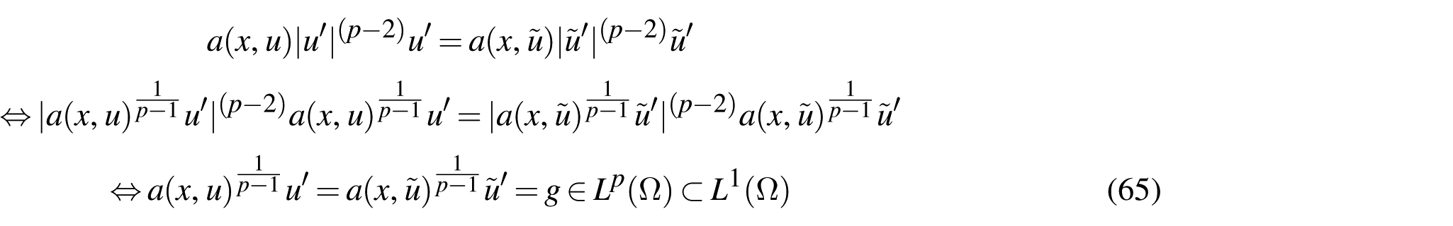
since the function $X\to |X{|}^{(p-2)}X$ is increasing. It is now clear that the function $X\to |X{|}^{-\frac{1}{(p-1)}}$ is $C^1$ on $(\lambda ,\mathrm{\Lambda })$ and thus if $a(x,u)$ is Lipschitz continuous in u so is $|a(x,u){|}^{-\frac{1}{(p-1)}}$ . Thus, from equation (65), we get easily

$$|u^{\prime }-{ũ}^{\prime }|=g(|a(x,u){|}^{-\frac{1}{(p-1)}}-|a(x,ũ){|}^{-\frac{1}{(p-1)}})\le C|g\parallel u-ũ|$$

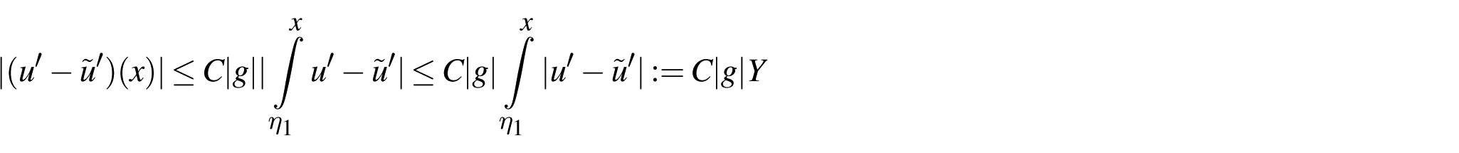
for some constant C. It follows that

$$|(u^{\prime }-{ũ}^{\prime })(x)|\le C|g\parallel \underset{{\eta }_1}{\overset{x}{\mathrm{\int }}}{u}^{\prime }-{ũ}^{\prime }|\le C|g|\underset{{\eta }_1}{\overset{x}{\mathrm{\int }}}|u^{\prime }-{ũ}^{\prime }|:=C|g|Y$$

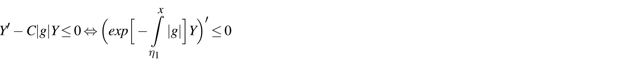
This can be written

$$Y^{\prime }-C|g|Y\le 0\iff (\exp [-\underset{{\eta }_1}{\overset{x}{\mathrm{\int }}}|g|]Y{)}^{\prime }\le 0$$

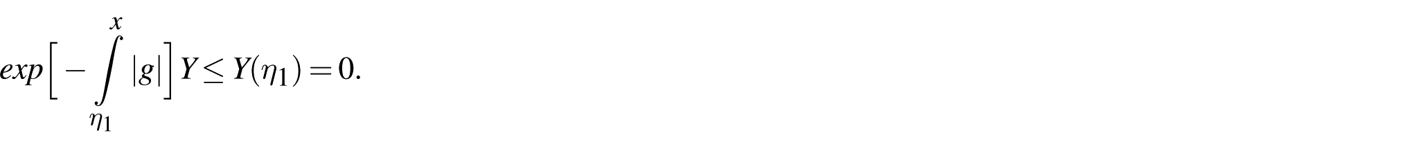
and thus

$$\exp [-\underset{{\eta }_1}{\overset{x}{\mathrm{\int }}}|g|]Y\le Y({\eta }_1)=0.$$

This implies that $u^{\prime }-{ũ}^{\prime }=0$ and $u=ũ$ . This completes the proof of uniqueness in this case.

To show the monotonicity in term of f, i.e., that $f_1\le f_2$ implies $u_1\le u_2$ , one uses (37). Then, in the method developed above, one replaces $({\eta }_1,{\eta }_2)$ by any connected component $({\eta }_1^{\prime },{\eta }_2^{\prime })$ of $\{u_1-u_2>0\}$ and shows that on such a component $u_1=u_2$ , which means it is empty. This completes the proof of the theorem. We refer to [6] for another proof. □

4. Variants, generalizations, existence

Let us set

$$A(x,u,\xi )=a(x,u)|\xi {|}^{p-2}\xi .$$

(66)

Noting the useful structure assumptions of this function used in Theorem 1, one can extend our result to $u_i$ solution to

$$\underset{\mathrm{\Omega }}{\mathrm{\int }}A(x,u_i,\mathrm{\nabla }{u}_i)\cdot \mathrm{\nabla }v+b(x,u_i)v=⟨f_i,v⟩$$

(67)

for all $v\in W_0^{1,p}(\mathrm{\Omega })$ , provided that A has suitable properties.

Indeed, suppose that $(x,u,\xi )\to A(x,u,\xi )$ is a Carathéodory function such that for some function $C\in L^{p^{\prime }}(\mathrm{\Omega })$ and some constants $C,C^{\prime }$

$$|A(x,u,\xi )|\le C(x)+C|u{|}^{p-1}+C^{\prime }|\xi {|}^{p-1}$$

(68)

then the integral (67) is well defined, recall that $||$ denotes the euclidean norm in ${\mathrm{ℝ}}^n$ .

From equation (67), we derive the analogue of equation (10) namely for any $v\in W_0^{1,p}(\mathrm{\Omega })$ , $v\ge 0$ ,

$$\begin{array}{ccc}\multicolumn{1}{c}{\underset{\mathrm{\Omega }}{\mathrm{\int }}(A(x,u_1,\mathrm{\nabla }{u}_1)}& \multicolumn{1}{c}{-A(x,u_1,\mathrm{\nabla }{u}_2))\cdot \mathrm{\nabla }v+(b(x,u_1)-b(x,u_1))v}& \multicolumn{1}{c}{}\\ \multicolumn{1}{c}{}& \multicolumn{1}{c}{\le \underset{\mathrm{\Omega }}{\mathrm{\int }}A(x,u_2,\mathrm{\nabla }{u}_2)-A(x,u_1,\mathrm{\nabla }{u}_2)\cdot \mathrm{\nabla }v}\end{array}$$

(69)

To get equation (13), it is enough to follow the steps (11), (12), assuming in addition that for some constant $A,C_p$

$$(A(x,u,\xi )-A(x,u,\zeta ))\cdot (\xi -\zeta )\ge C_p{(|\xi |+|\zeta |)}^{p-2}|\xi -\zeta {|}^2,$$

(70)

$$|A(x,u,\xi )-A(x,v,\xi )|\le A|u-v{|}^{\frac{1}{2}}|\xi {|}^{p-1},$$

(71)

for every $\xi ,\zeta ,u,v$ . This extends Theorem 1 in this more general case and also some result in [7]. The extension of Theorems 2, 3, 4, and 5 follows the same way as well as the arguments until theorem 6.

Instead of (66), one can also consider

$$A(x,u,\xi )=(a(x,u)|{\xi }_i{|}^{p-2}{\xi }_i)\mathrm{or}(a_i(x,u)|{\xi }_i{|}^{p_i-2}{\xi }_i)$$

(72)

the index i running from $i=1,\dots ,n$ . Consider first the case when

$$A(x,u,\xi )=(a(x,u)|{\xi }_i{|}^{p-2}{\xi }_i),p\le 2,a\mathrm{satisfying}(2),(7).$$

(73)

Then, one has

$$|A(x,u,\xi ){|}^2=\sum _i|a(x,u)|{\xi }_i{|}^{p-2}{\xi }_i{|}^2\le {\mathrm{\Lambda }}^2\sum _i|{\xi }_i{|}^{(p-1)2}\le {\mathrm{\Lambda }}^{2}n|\xi {|}^{(p-1)2}$$

(74)

and equation (68) holds. By equation (6), one has since $p-2\le 0$

$$\begin{array}{ccc}\multicolumn{1}{c}{(A(x,u,\xi )-A(x,u,\zeta ))\cdot }& \multicolumn{1}{c}{(\xi -\zeta )=a(x,u)\sum _i(|{\xi }_i{|}^{p-2}{\xi }_i-|{\zeta }_i{|}^{p-2}{\zeta }_i)({\xi }_i-{\zeta }_i)}& \multicolumn{1}{c}{}\\ \multicolumn{1}{c}{}& \multicolumn{1}{c}{\ge \lambda c_p\sum _i{(|{\xi }_i|+|{\zeta }_i|)}^{p-2}|{\xi }_i-{\zeta }_i{|}^2}\\ \multicolumn{1}{c}{}& \multicolumn{1}{c}{\ge \lambda c_p\sum _i{(|\xi |+|\zeta |)}^{p-2}|{\xi }_i-{\zeta }_i{|}^2=\lambda c_p{(|\xi |+|\zeta |)}^{p-2}|\xi -\zeta {|}^2}\\ \multicolumn{1}{c}{}\end{array}$$

(75)

which is equation (70). One has also

$$|A(x,u,\xi )-A(x,v,\xi ){|}^2=\sum _i{(a(x,u)-a(x,v))}^2{(|{\xi }_i{|}^{p-2}{\xi }_i)}^2\le n{A}^2|u-v\parallel \xi {|}^{(p-1)2}$$

(76)

which is equation (71). Thus, in this case, one can apply Theorem 3. Indeed, to sketch the proof, taking $v=F_{ϵ}(u_1-u_2)$ in equation (69), one gets by equations (75) and (76) the analogue of equations (25) and (26) namely for different constants C

$$\begin{array}{ccc}\multicolumn{1}{c}{I:=\lambda c_p\underset{S_{ϵ}}{\mathrm{\int }}\{|\mathrm{\nabla }{u}_1|+}& \multicolumn{1}{c}{|\mathrm{\nabla }{u}_2|{\}}^{p-2}\frac{|\mathrm{\nabla }(u_1-u_2){|}^2}{{\omega }^2(u_1-u_2)}+\{b(x,u_1)-b(x,u_2)\}{F}_{ϵ}(u_1-u_2)}& \multicolumn{1}{c}{}\\ \multicolumn{1}{c}{}& \multicolumn{1}{c}{\le C\underset{S_{ϵ}}{\mathrm{\int }}{\{|\mathrm{\nabla }{u}_1|+|\mathrm{\nabla }{u}_2|\}}^{\frac{p}{2}-1}\frac{|\mathrm{\nabla }(u_1-u_2)|}{\omega (u_1-u_2)}{\{|\mathrm{\nabla }{u}_1|+|\mathrm{\nabla }{u}_2|\}}^{\frac{p}{2}}}\\ \multicolumn{1}{c}{}& \multicolumn{1}{c}{\le \frac{\lambda c_p}{2}\underset{S_{ϵ}}{\mathrm{\int }}{\{|\mathrm{\nabla }{u}_1|+|\mathrm{\nabla }{u}_2|\}}^{p-2}\frac{|\mathrm{\nabla }(u_1-u_2){|}^2}{{\omega }^2(u_1-u_2)}+C\underset{S_{ϵ}}{\mathrm{\int }}{\{|\mathrm{\nabla }{u}_1|+|\mathrm{\nabla }{u}_2|\}}^p.}\\ \multicolumn{1}{c}{}\end{array}$$

Then, the end of the proof follows exactly the proof of Theorem 3 starting from equation (30).

On the other hand, (70) fails when $p>2$ , a satisfying (2). Indeed, consider the case when $n=2$ . Then, to verify the inequality (70), one will have to prove that for some constant C

$$a(x,u)\sum _{i=1}^2(|{\xi }_i{|}^{p-2}{\xi }_i-|{\zeta }_i{|}^{p-2}{\zeta }_i)({\xi }_i-{\zeta }_i)\ge C{(|\xi |+|\zeta |)}^{p-2}|\xi -\zeta {|}^2,$$

i.e., that

$$\frac{(|{\xi }_1{|}^{p-2}{\xi }_1-|{\zeta }_1{|}^{p-2}{\zeta }_1)}{{(|\xi |+|\zeta |)}^{p-2}|\xi -\zeta |}\frac{({\xi }_1-{\zeta }_1)}{|\xi -\zeta |}+\frac{(|{\xi }_2{|}^{p-2}{\xi }_2-|{\zeta }_2{|}^{p-2}{\zeta }_2)}{{(|\xi |+|\zeta |)}^{p-2}|\xi -\zeta |}\frac{({\xi }_2-{\zeta }_2)}{|\xi -\zeta |}\ge C.$$

(77)

In the case when ${\xi }_1={\zeta }_1$ , ${\xi }_2>{\zeta }_2$ , one has $({\xi }_2-{\zeta }_2)∕|\xi -\zeta |=1$ and the inequality reduces to

$$\frac{(|{\xi }_2{|}^{p-2}{\xi }_2-|{\zeta }_2{|}^{p-2}{\zeta }_2)}{{(|\xi |+|\zeta |)}^{p-2}|\xi -\zeta |}=\frac{(|{\xi }_2{|}^{p-2}{\xi }_2-|{\zeta }_2{|}^{p-2}{\zeta }_2)}{{\{{(|{\xi }_1{|}^2+|{\xi }_2{|}^2)}^{\frac{1}{2}}+{(|{\zeta }_1{|}^2+|{\zeta }_2{|}^2)}^{\frac{1}{2}}\}}^{p-2}|{\xi }_2-{\zeta }_2|}\ge C.$$

(78)

Having ${\xi }_2>{\zeta }_2$ fixed, it is clear that we get a contradiction when $|{\xi }_1|=|{\zeta }_1|\to \infty$ .

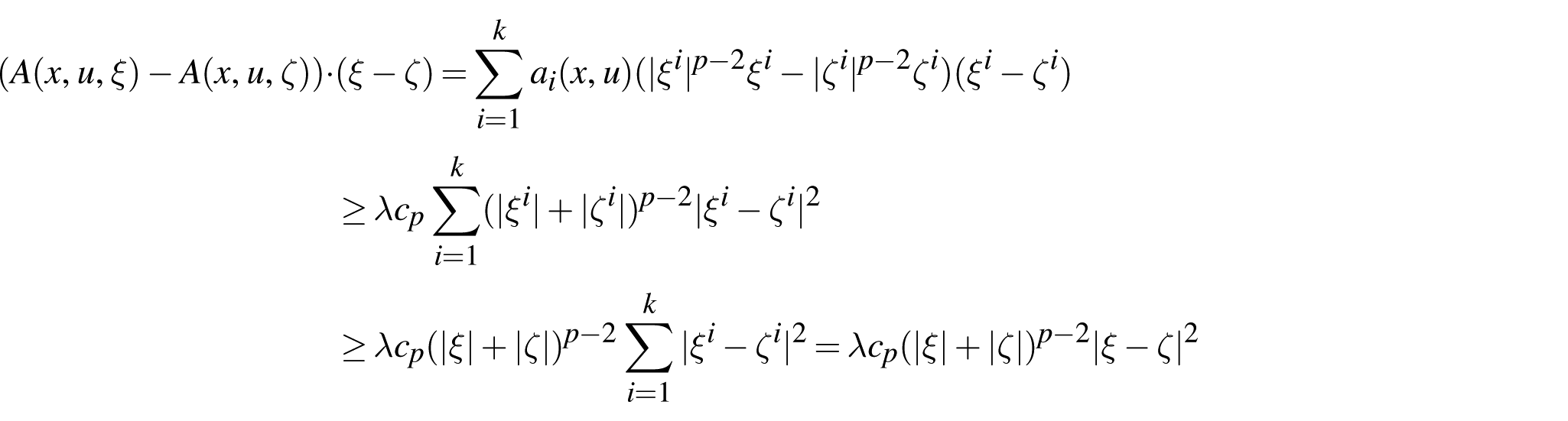
Thus, in the case, $p>2$ one has to proceed differently. We will consider the slightly more general case when

$$A(x,u,\xi )=(a_i(x,u)|{\xi }_i{|}^{p-2}{\xi }_i).$$

(79)

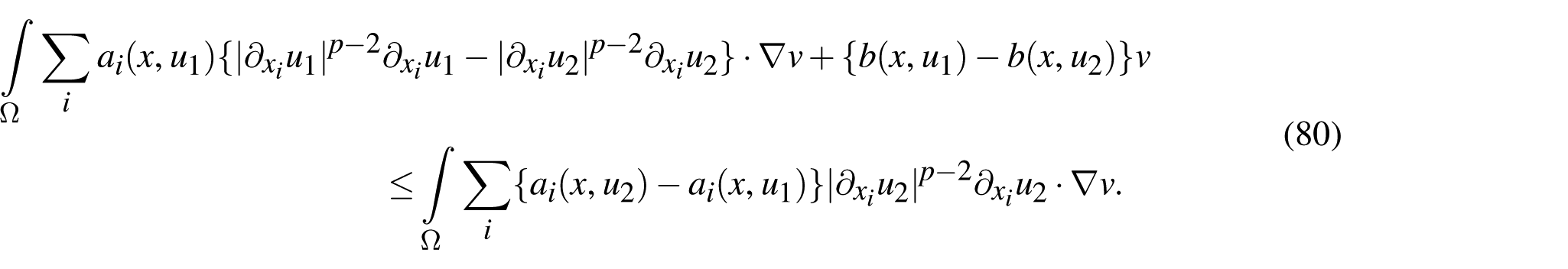
We suppose that each $a_i$ satisfies (2) and (7). Then if $u_i$ are solution to equation (67) one has in place of equation (10) for $v\in W_0^{1,p}(\mathrm{\Omega })$ , $v\ge 0$ ,

$$\begin{array}{ccc}\multicolumn{1}{c}{\underset{\mathrm{\Omega }}{\mathrm{\int }}\sum _i{a}_i(x,u_1)\{|{\partial }_{x_i}{u}_1{|}^{p-2}}& \multicolumn{1}{c}{{\partial }_{x_i}{u}_1-|{\partial }_{x_i}{u}_2{|}^{p-2}{\partial }_{x_i}{u}_2\}\cdot \mathrm{\nabla }v+\{b(x,u_1)-b(x,u_2)\}v}& \multicolumn{1}{c}{}\\ \multicolumn{1}{c}{}& \multicolumn{1}{c}{\le \underset{\mathrm{\Omega }}{\mathrm{\int }}\sum _i\{a_i(x,u_2)-a_i(x,u_1)\}|{\partial }_{x_i}{u}_2{|}^{p-2}{\partial }_{x_i}{u}_2\cdot \mathrm{\nabla }v.}\\ \multicolumn{1}{c}{}\end{array}$$

(80)

Choosing as before $v={(u_1-u_2)}^{+}\wedge ϵ$ , we get easily by equation (6) and the Young inequality, $S_{ϵ}$ being defined in equation (11),

$$\begin{array}{ccc}\multicolumn{1}{c}{\lambda c_p\underset{S_{ϵ}}{\mathrm{\int }}}& \multicolumn{1}{c}{\sum _i{\{|{\partial }_{x_i}{u}_1|+|{\partial }_{x_i}{u}_2|\}}^{p-2}{({\partial }_{x_i}(u_1-u_2))}^2+\{b(x,u_1)-b(x,u_2)\}v}& \multicolumn{1}{c}{}\\ \multicolumn{1}{c}{}& \multicolumn{1}{c}{\le \underset{S_{ϵ}}{\mathrm{\int }}\sum _{i}A|u_1-u_2{|}^{\frac{1}{2}}|{\partial }_{x_i}{u}_2{|}^{p-1}|{\partial }_{x_i}(u_1-u_2)|}\\ \multicolumn{1}{c}{}& \multicolumn{1}{c}{\le \underset{S_{ϵ}}{\mathrm{\int }}\sum _{i}A|u_1-u_2{|}^{\frac{1}{2}}{(|{\partial }_{x_i}{u}_1|+|{\partial }_{x_i}{u}_2|)}^{\frac{p}{2}}{(|{\partial }_{x_i}{u}_1|+|{\partial }_{x_i}{u}_2|)}^{\frac{p}{2}-1}|{\partial }_{x_i}(u_1-u_2)|}\\ \multicolumn{1}{c}{}& \multicolumn{1}{c}{\le \underset{S_{ϵ}}{\mathrm{\int }}\sum _i\frac{\lambda c_p}{2}{\{|{\partial }_{x_i}{u}_1|+|{\partial }_{x_i}{u}_2|\}}^{p-2}{({\partial }_{x_i}(u_1-u_2))}^2}\\ \multicolumn{1}{c}{}& \multicolumn{1}{c}{+\underset{S_{ϵ}}{\mathrm{\int }}\sum _i\frac{1}{2\lambda c_p}{A}^2ϵ{(|{\partial }_{x_i}{u}_1|+|{\partial }_{x_i}{u}_2|)}^p.}\\ \multicolumn{1}{c}{}\end{array}$$

(81)

Then, it follows that

$$\underset{S_{ϵ}}{\mathrm{\int }}\{b(x,u_1)-b(x,u_2)\}\mathrm{vdx}\le ϵ\frac{1}{2\lambda c_p}{A}^2\underset{S_{ϵ}}{\mathrm{\int }}\sum _i{(|{\partial }_{x_i}{u}_1|+|{\partial }_{x_i}{u}_2|)}^p\mathrm{dx}$$

(82)

and one concludes as in the end of Theorem 1. We left to the reader the proofs of the analogue of theorems of section 2 or 3.

Remark 3. When $p>2$ assumption (70) can thus be replaced by the weaker one below

$$(A(x,u,\xi )-A(x,u,\zeta ))\cdot (\xi -\zeta )\ge C_p\sum _{i=1}^n{(|{\xi }_i|+|{\zeta }_i|)}^{p-2}|{\xi }_i-{\zeta }_i{|}^2.$$

(83)

To end this section, we would like to come up with an existence result for almost all the problems investigated above. If ξ is a vector of ${\mathrm{ℝ}}^n$ we suppose it split in k different sets of components in such a way it can be written

$$\xi =({\xi }^1,{\xi }^2,\dots ,{\xi }^k).$$

(84)

Then, if $a_i(x,u)$ are k Carathéodory functions satisfying (2) we set

$$A(x,u,\xi )=(a_i(x,u)|{\xi }^i{|}^{p-2}{\xi }^i).$$

(85)

Note that if $k=1$ , ${\xi }^1=\xi$ and if $k=n$ , ${\xi }^i={\xi }_i$ (cf. equation (72)). We can now consider the problem of finding u solution to

$$\{\begin{array}{c}\multicolumn{1}{c}{u\in W_0^{1,p}(\mathrm{\Omega }),}\\ \multicolumn{1}{c}{{\int }_{\mathrm{\Omega }}A(x,u,\mathrm{\nabla }u)\cdot \mathrm{\nabla }v+b(x,u)v=⟨f,v⟩\mathrm{\forall }v\in W_0^{1,p}(\mathrm{\Omega }).}\end{array}$$

(86)

Suppose that $u\to b(x,u)$ satisfies (3) and defines a continuous mapping from $L^p(\mathrm{\Omega })$ into $L^{p^{\prime }}(\mathrm{\Omega })$ . Then, we have

Theorem 7. Under the assumptions above, suppose in addition that $b(x,0)=0$ , then for $f\in W^{-1,p^{\prime }}(\mathrm{\Omega })$ , there exists at least one solution to equation (86).

Proof. Consider $w\in L^p(\mathrm{\Omega })$ . Then, we claim that there exists a unique $u=S(w)$ solution to

$$\{\begin{array}{c}\multicolumn{1}{c}{u\in W_0^{1,p}(\mathrm{\Omega }),}\\ \multicolumn{1}{c}{{\int }_{\mathrm{\Omega }}A(x,w,\mathrm{\nabla }u)\cdot \mathrm{\nabla }v+b(x,u)v=⟨f,v⟩\mathrm{\forall }v\in W_0^{1,p}(\mathrm{\Omega }).}\end{array}$$

(87)

First we note that

$$⟨\mathcal{A}(u),v⟩=\underset{\mathrm{\Omega }}{\mathrm{\int }}A(x,w,\mathrm{\nabla }u)\cdot \mathrm{\nabla }v+b(x,u)v$$

(88)

defines a linear form of $W^{-1,p^{\prime }}(\mathrm{\Omega })$ . Indeed, the components of $A(x,w,\mathrm{\nabla }u)$ are all of the type $a_i(x,u)|{(\mathrm{\nabla }u)}^i{|}^{p-2}{\partial }_{x_j}u$ and thus are all bounded by $\mathrm{\Lambda }|\mathrm{\nabla }u{|}^{p-1}$ . It follows that

$$|A(x,w,\mathrm{\nabla }u)|\le n\mathrm{\Lambda }|\mathrm{\nabla }u{|}^{p-1}\in L^{p^{\prime }}(\mathrm{\Omega }).$$

(89)

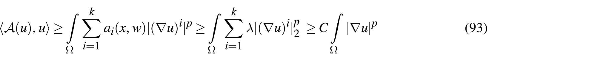
Thus, $\mathcal{A}$ is an operator from $W_0^{1,p}(\mathrm{\Omega })$ into its dual. We claim that it is coercive. To prove this, if we denote by

$$|x{|}_p=\{\sum _{i=1}^m|x_i{|}^p{\}}^{\frac{1}{p}}.$$

(90)

the p-norms in ${\mathrm{ℝ}}^m$ we are going to use the equivalence of these norms in different finite-dimensional spaces ${\mathrm{ℝ}}^m$ . Indeed, for different constants, we have then

$$\{\sum _{i=1}^k|{\xi }^i{|}_2^p{\}}^{\frac{1}{p}}\ge c_1\sum _{i=1}^k|{\xi }^i{|}_2\ge c_1{c}_2\sum _{i=1}^k|{\xi }^i{|}_1=c_1{c}_2|\xi {|}_1\ge c_1{c}_2{c}_3|\xi {|}_2,$$

(91)

i.e.,

$$\sum _{i=1}^k|{\xi }^i{|}_2^p\ge C|\xi {|}_2^p.$$

(92)

Thus, taking $v=u$ in equation (88), it comes (recall that $||=|{|}_2$ )

$$⟨\mathcal{A}(u),u⟩\ge \underset{\mathrm{\Omega }}{\mathrm{\int }}\sum _{i=1}^k{a}_i(x,w)|{(\mathrm{\nabla }u)}^i{|}^p\ge \underset{\mathrm{\Omega }}{\mathrm{\int }}\sum _{i=1}^k\lambda |{(\mathrm{\nabla }u)}^i{|}_2^p\ge C\underset{\mathrm{\Omega }}{\mathrm{\int }}|\mathrm{\nabla }u{|}^p$$

(93)

and the coerciveness follows.

Remark 4. It is clear that ${\xi }^i$ could also be a vector built with certain components of ξ provided that at the end they are all used at least once, i.e., the operator at hand could be an operator sum of operators involving p-Laplace operators in dimension less than n.

It is clear that $\mathcal{A}$ is in addition monotone, continuous on finite-dimensional subspaces. Thus, the existence of a unique solution to equation (87) follows from classical arguments (cf. for instance, [2,3,13,14]). Next, if we show that S has a fixed point, we will have obtained a solution to equation (86). For that we consider S as a mapping from $L^p(\mathrm{\Omega })$ into itself. From equations (93) and (87), if $u=S(w)$ , we have ( $|f{|}_{-1,p^{\prime }}$ denotes the strong dual norm in $W^{-1,p^{\prime }}(\mathrm{\Omega }))$

$$C\underset{\mathrm{\Omega }}{\mathrm{\int }}|\mathrm{\nabla }u{|}^p\le ⟨\mathcal{A}(u),u⟩\le ⟨f,u⟩\le |f{|}_{-1,p^{\prime }}\{\underset{\mathrm{\Omega }}{\mathrm{\int }}|\mathrm{\nabla }u{|}^p{\}}^{\frac{1}{p}},$$

(94)

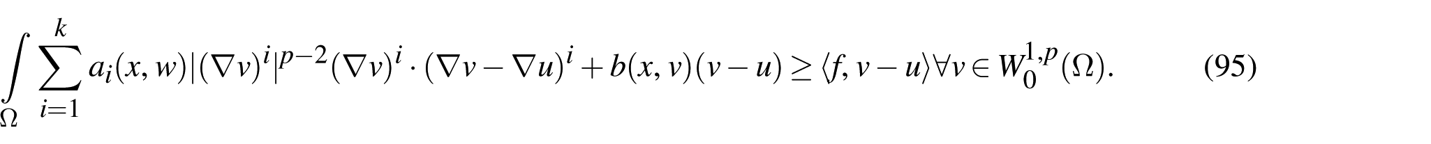
i.e., ${\{{\int }_{\mathrm{\Omega }}|\mathrm{\nabla }u{|}^p\}}^{\frac{1}{p}}$ is bounded independently of w. If S is continuous, it will be compact and the existence of a fixed point will be just a consequence of the Schauder fixed point theorem. Thus, we just have now to prove the continuity of S. To do that one follows the lines of Proposition 3.1. Indeed, first one shows easily that equation (87) is equivalent to

$$\underset{\mathrm{\Omega }}{\mathrm{\int }}\sum _{i=1}^k{a}_i(x,w)|{(\mathrm{\nabla }v)}^i{|}^{p-2}{(\mathrm{\nabla }v)}^i\cdot {(\mathrm{\nabla }v-\mathrm{\nabla }u)}^i+b(x,v)(v-u)\ge ⟨f,v-u⟩\mathrm{\forall }v\in W_0^{1,p}(\mathrm{\Omega }).$$

(95)

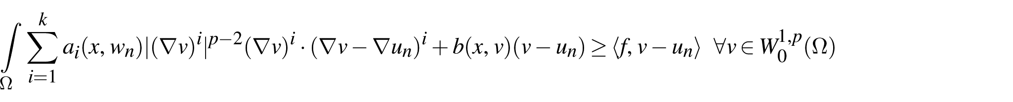
Then, one considers $w_n\in L^p(\mathrm{\Omega })$ such that $w_n\to w\in L^p(\mathrm{\Omega })$ . One sets $u_n=S(w_n)$ . Since by equation (94) $u_n$ is bounded independently of n one can extract a subsequence still labeled $u_n$ such that for some $u\in W_0^{1,p}(\mathrm{\Omega })$ , $u_n\rightharpoonup u$ in $W_0^{1,p}(\mathrm{\Omega })$ and

$$u_n\to u\mathrm{in}{L}^p(\mathrm{\Omega })\mathrm{and}\mathrm{a.e.}\mathrm{in}\mathrm{\Omega },\mathrm{\nabla }{u}_n\rightharpoonup \mathrm{\nabla }u\mathrm{in}{L}^p(\mathrm{\Omega }).$$

(96)

Then, passing in the limit in

$$\underset{\mathrm{\Omega }}{\mathrm{\int }}\sum _{i=1}^k{a}_i(x,w_n)|{(\mathrm{\nabla }v)}^i{|}^{p-2}{(\mathrm{\nabla }v)}^i\cdot {(\mathrm{\nabla }v-\mathrm{\nabla }{u}_n)}^i+b(x,v)(v-u_n)\ge ⟨f,v-u_n⟩\mathrm{\forall }v\in W_0^{1,p}(\mathrm{\Omega })$$

one sees that u is the unique solution to equation (95) i.e. $u=s(w)$ . By uniqueness of the limit, the whole sequence $u_n$ converges toward u and S is continuous. This completes the proof of the theorem. □

Remark 5. Of course, for the operators introduced in Theorem 7, some uniqueness results or monotonicity with respect to f are available. They follow the lines developed above and their proofs are left to the reader. To be convinced of these possibilities note that if $A(x,u,\xi )$ is given by equation (85) it holds, for instance, when $a_i$ satisfies (2) and $p\le 2$

$$\begin{array}{ccc}\multicolumn{1}{c}{(A(x,u,\xi )-A(x,u,\zeta ))\cdot }& \multicolumn{1}{c}{(\xi -\zeta )=\sum _{i=1}^k{a}_i(x,u)(|{\xi }^i{|}^{p-2}{\xi }^i-|{\zeta }^i{|}^{p-2}{\zeta }^i)({\xi }^i-{\zeta }^i)}& \multicolumn{1}{c}{}\\ \multicolumn{1}{c}{}& \multicolumn{1}{c}{\ge \lambda c_p\sum _{i=1}^k{(|{\xi }^i|+|{\zeta }^i|)}^{p-2}|{\xi }^i-{\zeta }^i{|}^2}\\ \multicolumn{1}{c}{}& \multicolumn{1}{c}{\ge \lambda c_p{(|\xi |+|\zeta |)}^{p-2}\sum _{i=1}^k|{\xi }^i-{\zeta }^i{|}^2=\lambda c_p{(|\xi |+|\zeta |)}^{p-2}|\xi -\zeta {|}^2}\end{array}$$

which is equation (70).