Stochastic modelling of elasticity tensor fields

Abstract

We present a novel framework for the probabilistic modelling of random fourth-order material tensor fields, with a focus on tensors that are physically symmetric and positive definite (SPD), of which the elasticity tensor is a prime example. Given the critical role that spatial symmetries and invariances play in determining material behaviour, it is essential to incorporate these aspects into the probabilistic description and modelling of material properties. In particular, we focus on spatial point symmetries or invariances under rotations, a classical subject in elasticity. Following this, we formulate a stochastic modelling framework using a Lie algebra representation via a memory-less transformation that respects the requirements of positive definiteness and invariance. With this, it is shown how to generate a random ensemble of elasticity tensors that allows an independent control of strength, eigenstrain, and orientation. The procedure also accommodates the requirement to prescribe specific spatial symmetries and invariances for each member of the whole ensemble, while ensuring that the mean or expected value of the ensemble conforms to a potentially ‘higher’ class of spatial invariance. Furthermore, it is important to highlight that the set of SPD tensors forms a differentiable manifold, which geometrically corresponds to an open cone within the ambient space of symmetric tensors. Thus, we explore the mathematical structure of the underlying sample space of such tensors and introduce a new distance measure or metric, called the ‘elasticity metric’, between the tensors. Finally, we model and visualize a one-dimensional spatial field of orthotropic Kelvin matrices using interpolation based on the elasticity metric.

1. Introduction

The computational modelling of heterogeneous materials often has to resort to a statistical or probabilistic description, as the precise details are unknown or uncertain. The material properties are usually collected in tensor quantities, and these tensors are often of even order, and due to Onsager’s reciprocity relations [1] physically symmetric—in elasticity this is termed the major symmetry—and in addition, they are frequently positive definite as they are associated with, e.g., stored energy or entropy production [2]. This class of even-order physically symmetric and positive definite (SPD) tensors—and here especially the important class of fourth-order tensors and their associated symmetry classes—is the main focus in this contribution. The stochastic modelling procedure we shall describe is applicable to any such even-order physically symmetric and possibly additionally positive definite tensor, but we shall spell things out in detail for fourth-order SPD tensors, a prime example of which is the elasticity tensor, which will be taken here to stand for all such tensors.

Well known examples of such SPD tensors are, e.g., thermal conductivity—a second-order tensor mapping temperature gradients to thermal fluxes—or, as already mentioned above, the elasticity tensor of a linearly elastic material as a fourth-order tensor, mapping strains to stresses. A sixth order more involved example is the complete piezo-elasticity tensor, mapping the combination of strains and electric displacement to stress and electric field. Such a tensor of a coupled problem would be best tackled using the tensor-block matrices of Nikabadze [3], which would be a more or less straightforward extension of the concepts treated here.

The representation and stochastic modelling of second-order tensors, such as those describing diffusion phenomena, was shown in a precursor paper [4]. Here we want to follow along the general lines of this approach based on the spectral decomposition and symmetry-group reduction, but for higher-order tensors, a novel situation arises, namely the situation that the symmetry-group reduction [5–7] cannot diagonalise the tensor. We outline the general idea for SPD tensors of any even order but concentrate in detail on fourth-order tensors.

As the interest here is in the probabilistic modelling of such tensors, a simple way to realise this is to think of the tensor entries as random variables. But an important aspect of a material law described by such a tensor is its invariance under spatial symmetries [5–10]. Although the numerical values of the tensor entries may be uncertain resp. random variables, it is not uncommon that the class of spatial symmetries is known exactly, both for each individual realisation as well as for the mean. These invariances under spatial symmetries are a classical subject [11], and the different symmetry groups allow one to assign such material laws, resp. the tensors describing them into certain classes, e.g., like the well-known isotropic class, or the orthotropic class of materials. Second-order tensors in 3D show, next to these just mentioned invariance resp. symmetry classes of iso- or ortho-tropy, additionally only plan-isotropic behaviour [4,11]. Fourth-order spatial tensors, however, have a richer set of symmetry classes than second-order tensors [11–13], namely eight symmetry or invariance classes in 3D [14], and four in 2D [15], cf. also the general references [8–10].

Any even-order tensor may be viewed as a linear map when acting on the space of tensors of half the order by contracting over half the indices [16–18]. In the case of the fourth-order elasticity tensor, this space of tensors half the order is the space of strains, i.e., second-order symmetric tensors, as the elasticity tensor maps a strain tensor into the corresponding stress tensor. By choosing appropriate bases in the vector space of tensors of half the order [16], this linear map can be represented by a matrix; so the class of tensors we are interested in can thus be represented by SPD matrices. We shall switch to this matrix representation whenever it is convenient to do so. The spatial invariance resp. symmetry groups are then realised as linear transformation groups on the relevant space of half-order tensors, or, equivalently, on the space underlying the representing symmetric matrices just mentioned. These transformation groups then define invariant subspaces of the SPD matrix representing the tensor [5–7]. By transforming into a basis adapted to these invariant subspaces, the matrix takes on a block-diagonal form. This transformation to block-diagonal form is termed the symmetry resp. invariance group reduction or decomposition. Here we shall prefer the term ‘invariance’ of the tensor resp. matrix under the spatial group operations over the term ‘symmetry’, in order to avoid confusion with the physical symmetry due to Onsager’s reciprocity relations, which results in symmetric matrices.

Any SPD matrix or linear map can be spectrally decomposed with positive eigenvalues and has orthogonal eigenvectors. This spectral eigenvalue/-vector (EV) decomposition separates the size, strength, or stiffness information contained in the eigenvalues from the information about the orientation of the eigenvectors. For the sake of brevity and simplicity, in the following, we shall speak about the eigenvalues in terms of stiffness or elastic moduli as they apply to the elasticity or Hooke tensor, but obviously this can be easily translated to any other physical property. The group reduction together with the spectral decomposition are the main building blocks of our approach. In the representation proposed, and in this, we see one of the novelties of our approach, we want to keep the modelling of strength/stiffness, eigenstrain distribution, and spatial orientation separate and thus be able to control it independently. So, finally, one ends up considering random SPD matrices, where certain invariances are known for the whole population, as well as for the mean. There is already extensive work on random matrices, drawing on several sources, which is mentioned only very briefly here [19–22].

The separation of stiffness, eigenstrains, and spatial orientation information is actually an old subject, as the characterisation of elasticity tensors through their eigenvalues resp. moduli was already started by Stokes (cf. Nikabadze [3], Love [23], Todhunter and Pearson [24]) and Lord Kelvin (W.K. Thomson) [25,26]. It was little appreciated at the time and then apparently almost forgotten, to be picked up again about a century later by Fedorov [27], and subsequently among others [2,3,18,28–43]. Kelvin originally used this to classify material symmetries; a historical account may be found in studies by Helbig [44,45]. It is an early example of a tensor representation through an orthogonal tensor decomposition, and many other such representations and decompositions have been considered; a compilation and comparison of different orthogonal decompositions may be found in literature [46–48]. Furthermore, topics of tensor representation are also treated in previous studies [11,49–51], and more information on tensor decompositions may also be found in literature [16,52–65]. The representation preferred by us, based on the spectral decomposition referred to above, offers the possibility of separately modelling stiffness, orientation, and possibly the eigenstrain, as well as separately controlling their individual probability distributions. Relative to existing models this offers a direct and fine control of those properties, while being free of any limitations. It additionally offers direct control of the symmetry resp. invariance properties to be discussed below, both of the ensemble mean and of each individual realisation. This feature distinguishes our approach from existing models. This and further distinctions are discussed in more detail by Shivanand et al. [4] and will not be repeated here.

It is well known that there are eight symmetry or invariance classes for symmetric fourth-order tensors in 3D, they may be found in the references just quoted, as well as in the reference works [8–10]. To sketch the connection of the spectral or EV-decomposition with the idea of invariance under symmetry groups, it was already mentioned that one considers the representation of the elasticity tensor as a linear map through a proper choice of a basis in the space of strains. In the case of the elasticity tensor, this is known as the Kelvin notation. The eigenvalues of the Kelvin matrix are traditionally called Kelvin moduli and the corresponding eigenvectors Kelvin modes.

The invariance class of the material or elasticity tensor is identified by rotating the coordinate system of the physical space in such a way as to introduce as many zeros as possible in the tensor. This pattern then turns out to be stable under a whole subgroup of rotations, which is the point invariance resp. symmetry group of the material resp. the tensor or the Kelvin matrix. This process of group reduction is an algorithm to find orthogonal invariant subspaces which reduce the matrix to block-diagonal form [5,6], thereby also identifying the invariance resp. symmetry group. For fourth-order tensors resp. Kelvin matrices this group is represented as a subgroup of the group of orthogonal transformations on strain-space [11,51,66,67]. It also determines the eigenstrain distribution in the relevant elasticity class [12,13,35,68,69].

The group-reduced block-diagonal form alluded to above is the representation usually chosen in the literature when the different elasticity classes are discussed [8–13]. The block-diagonal form of the matrix can be further reduced to diagonal form in each block with a orthogonal transformation to a direct sum of specific eigenstrain subspaces. This last orthogonal transformation in strain-space does not result from a spatial rotation but is purely in strain-space. This consideration of iso-spectral eigenstrain distributions is a crucial extension to higher-order tensors of the analogous development in Shivanand et al. [4] for second-order tensors.

The fourth-order elasticity tensor may thus be represented in a two-stage procedure by a combined group reduction and spectral decomposition, i.e., one may represent the elasticity tensor in form of the Kelvin matrix by a positive diagonal matrix of eigenvalues resp. Kelvin moduli, an ‘eigenstrain distributor’ rotation within an invariant subspace of the block-diagonal form, and the spatially induced rotation for the symmetry group reduction. The task of representing random SPD tensor fields thus is reduced to representing these three components. It is worthwhile, and in our context essential, to observe that these three ingredients —spatially induced orthogonal transformations for the group reduction, general orthogonal transformation on strain-space to diagonalise each block, and diagonal SPD matrices of Kelvin moduli—are each members of matrix Lie groups.

In the modelling of random tensor fields, the most comfortable and desirable way is to find an unconstrained representation on a linear vector space. For the purpose of modelling or representing a random SPD tensor, a geometric point of view might be helpful. In the vector space of physically symmetric tensors of a given even order, the positive definite ones (SPD tensors) form an open convex cone, i.e., sums of SPD tensors with positive coefficients are again SPD tensors. They thus form a differentiable manifold, but not a vector space. So the desire is to represent this cone on a vector space without any constraints. One such possibility is the matrix exponential and logarithm [4,70–72], and this can be used in different guises, and will also be used here. The Lie groups just alluded to—diagonal SPD matrices and subgroups of orthogonal matrices—which we want to use in the representation, as the they allow one to independently model different aspects of the SPD tensor, are geometrically speaking more complicated than the simple vector space of physically symmetric tensors. But the exponential and logarithm may be used in this situation as well—here coinciding with the Lie group exponential and logarithm—and furnish a representation on the associated Lie algebra of the corresponding group, which is geometrically the tangent space at the group identity; effectively giving a representation on a direct sum of linear spaces.

In this context, it is worthwhile to note that the nature of the set of SPD tensors—a differentiable manifold which is geometrically an open cone in the ambient space of symmetric tensors—suggests that the calculation of averages, means, or expected values inherited from this ambient space based on a Euclidean metric is not the natural one to use. It has actually been observed that using the mean based on the Euclidean metric has some undesirable properties [73–82], in particular the so-called swelling, fattening, and shrinking effects [20,70–72,82,83].

To wit, when finding the midpoint (average) or interpolating between two points on earth’s surface, one will usually not mean the midpoint of a straight connecting line (the average of the ambient Euclidean space), but the intrinsic midpoint half way on a great circle. This intrinsic kind of average or mean using a non-Euclidean metric is called a Fréchet mean, and will be shortly recapped in Appendix 1, recalling the connection between metric and averaging. From a metric, one may define variationally the Fréchet or Karcher mean—a generalisation of the arithmetic resp. Euclidean distance based mean, see Appendix 1—to more general metric spaces [84]. This is an area of active research [82,85–89], and the ‘best’ metric and mean seem to be application dependent.

The effect of using a mean which is not adapted to the manifold can have various consequences. When modelling a non-isotropic material, this may mean a loss of anisotropy for the mean, which may be undesirable in some situations. In the above literature—particularly that coming from the medical field of diffusion tensor imaging, where these undesirable effects are not acceptable, but also in the estimation of covariance matrices—there is discussion on what metric to use [60,71,74–76,79,82,88–95]. For elasticity tensors, this topic of a metric has also attracted some attention [4,12,81,96–101], e.g., in finding the closest elasticity tensor of some invariance class to measurement data.

We formulate some desiderata for a mean resp. a metric for the case of elasticity. This will be connected to the proposed representation on a direct sum of Lie algebras, which allows one to choose inner products on the Lie algebras to define a metric, which is transported via the exponential map to the Lie group and hence gives rise to a Riemannian structure on the group, which can then be used to define a metric—which we suggest to call the ‘elasticity metric’—on the cone of positive definite tensors which satisfies the proposed desiderata; the details of this are to be found in the Appendix 1. Based on this distance one may then formulate the corresponding Fréchet mean, which may be called the ‘elasticity mean’.

To generate random SPD matrices, a reduced non-parametric approach taking account of positive definiteness was presented by Soize [21,102]. Here the algebraic property that positive elements in the algebra are squares of other elements in the algebra [103,104] is used to ascertain positive definiteness. This then forms the basis for the generation of random elasticity tensors with specified invariance in the mean and fully anisotropic invariance in each realisation, resp. controlled elasticity class invariance with constant spatial orientation of the symmetry axes in each realisation, which is shown in a series of papers [105–113].

In the area of modelling of random tensor fields with given invariance properties, the culmination of a long series of works [51,66,67,114,115] is reported in Malyarenko and Ostoja-Starzewski [11], specifically looking at stochastically homogeneous and isotropic random tensor fields of any order in a three-dimensional domain. The spatial modelling uses the spectral theorem for the covariance function, to generate a spectral or Karhunen-Loève like representation (e.g. Matthies [116]) of the random tensor field with the desired invariance properties. No particular attention is paid to positive definiteness, as the methods used are purely vector space like, such as linear combinations or series and integrals. The danger is here that although the limiting expression may well represent a positive definite tensor, in a practical computational situations these series and integrals have to be truncated resp. numerically approximated, and this step may lead to an unacceptable numerical loss of positive definiteness everywhere. In some associated numerical examples of anti-plane shear [117], positive definiteness everywhere is obtained by using a deterministic SPD base tensor and adding a random rank-one tensor—a dyadic or tensor product of identical vectors and thus automatically positive—and controlling the random coefficient so that the sum stays SPD. Here we shall also use a Karhunen-Loève like field model to represent the parameters in the Lie algebras mentioned above, but by modelling the logarithm of the tensor one can ensure positive definiteness everywhere via the exponential map for each realisation at each point in space.

Ensuring positive definiteness everywhere through the use of the exponential function, resp. the logarithm in the opposite direction, is an often used approach; it typically based on the spectral or EV-decomposition. As the spectral decomposition may be written as a sum of dyadic or tensor products of eigenvectors, this furnishes a connection to the above mentioned approach in Zhang et al. [117]. The exponential function is employed in previous studies [4,70–72,83,88,109,111], and it may be combined with the squaring approach [109,111,118] to ensure compliance with a particular invariance class. This log-modelling is quite common when measuring diffusion and conductivity tensors, i.e., focusing the description on the logarithm of the tensor. This takes advantage of the fact that the invariance classes are the same for a tensor and its exponential resp. logarithm. Also in this work, the exponential function is used in an essential way to ensure positive definiteness numerically in each realisation. The exponential function may be even used to model the rotations, essentially parametrising the angles [118]. Here we follow [4] and consequently model the eigenvalues and the rotations via the exponential function, mapping from a Lie algebra to the corresponding Lie group

The structure of the paper is outlined as follows: Section 2 collects essential preliminaries, including the notation for even-order tensors in Section 2.1 and Kelvin’s matrix representation of Hooke’s law in Section 2.2, with further details provided in Appendix 3. Section 2.3 discusses the transformation of the Kelvin matrix under rotations and briefly addresses how spatial rotations are modelled in the sequel and how they influence the strain-space. Additional background on rotations can be found in Appendix 2. This section also introduces the reduction of the Kelvin matrix to block diagonal form, its spectral decomposition, and the formulation of group invariance in elasticity. In order to make this work more easily accessible, the group theoretic material will be kept to a minimum. The representation and modelling of fourth-order SPD tensor fields, based on fields of parameters, is detailed in Section 2.4.

The main part of the paper is Section 3, where Section 3.1 covers the Lie representation of the Kelvin matrix, and Section 3.2 introduces the concept of a Fréchet mean for SPD tensors. This uses the proposed ‘elasticity metric’ which is described in Appendix 1. In Section 3.3, we formulate our requirements for a representation of SPD tensors, as well as some general thoughts and desiderata on how to average SPD tensors based on Fréchet means. Next, in Section 3.4, we introduce the framework for generating random ensembles of Kelvin matrices at a spatial point, followed by a description of spatial variation. The focus here is on modelling randomness through the separation of stiffness, eigenstrains, and spatial orientation. Section 4 explores Kelvin’s spectral decomposition of Hooke’s law in detail, with the relationship to 2D and 3D elasticity classes covered in Section 4.1 and Section 4.2, respectively. Finally, the paper concludes in Section 5.

2. Preliminaries

We consider physical space as given by $\mathcal{V}\equiv {\mathrm{ℝ}}^d$ , the physically interesting instances being the 2D situation with $d=2$ , and the full 3D case with $d=3$ . For the sake of simplicity, we shall consider only Cartesian coordinate systems and orthonormal bases, so we do not distinguish co- and contra-variant indices.

2.1. Even order tensors as linear maps

Vectors in $\mathcal{V}$ like the position vector are denoted as $\mathit{x}=(x_i)\in \mathcal{V}$ , whereas second-order tensors (matrices) are denoted as $\mathsf{Q}=(Q_{\mathrm{ik}})\in \mathcal{V}\otimes \mathcal{V}={\mathcal{V}}^{\otimes 2}$ , which will be identified with linear maps $ℒ(\mathcal{V})$ on $\mathcal{V}$ via the matrix-vector product by $\mathit{y}=(y_i)=\mathsf{Q}\mathit{x}=(Q_{\mathrm{ik}}{x}_k)$ (Einstein’s summation convention used).

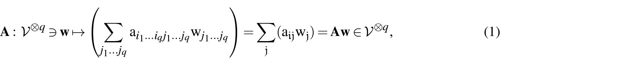
Tensors of higher order than two will be denoted as $\mathbf{w}={\mathrm{w}}_{i_1{i}_2{i}_3\dots i_q}={\mathrm{w}}_{\mathfrak{i}}\in {\mathcal{V}}^{\otimes q}$ for a tensor of order q. Considering a tensor of even order, say $2q$ : $\mathbf{a}=({\mathrm{a}}_{i_1{i}_2{i}_3\dots i_q{j}_1{j}_2{j}_3\dots j_q})=({\mathrm{a}}_{\mathfrak{i}\mathfrak{j}})\in {\mathcal{V}}^{\otimes 2q}$ —where for ease of notation we have used a multi-index $\mathfrak{i}=(i_1{i}_2{i}_3\dots i_q)\in {\mathrm{\mathbb{N}}}^q$ — it can be naturally be viewed as a linear map $\mathbf{A}\in ℒ({\mathcal{V}}^{\otimes q})$ on the space of tensors of half the order, by contracting the tensor product of $\mathbf{a}$ and $\mathbf{w}$ over the last q indices, thereby implicitly using the canonical Euclidean inner product to be introduced below:

$$\mathbf{A}:{\mathcal{V}}^{\otimes q}\ni \mathbf{w}\mapsto \left(\sum _{j_1\dots j_q}{\mathrm{a}}_{i_1\dots i_q{j}_1\dots j_q}{\mathrm{w}}_{j_1\dots j_q}\right)=\sum _{\mathfrak{j}}({\mathrm{a}}_{\mathfrak{i}\mathfrak{j}}{\mathrm{w}}_{\mathfrak{j}})=\mathbf{A}\mathbf{w}\in {\mathcal{V}}^{\otimes q},$$

(1)

where the last sum is particularly suggestive, as it is a matrix-vector multiplication with multi-indices. By choosing bases in ${\mathcal{V}}^{\otimes 2q}$ , or, equivalently, by ordering the multi-indices in some way, one may easily constructs a matrix representation for the map $\mathbf{A}$ . For the elasticity tensor, this will be done in Section 2.2 by using the so-called Kelvin notation.

2.1.0.1. Inner product and symmetry

The canonical Euclidean inner product for $\mathit{x},\mathit{y}\in \mathcal{V}\equiv {\mathrm{ℝ}}^d$ is denoted by $\mathit{x}\cdot \mathit{y}={\mathit{x}}^{\mathsf{T}}\mathit{y}=⟨\mathit{x},\mathit{y}⟩:=x_i{y}_i$ . This induces an inner product for general tensors $\mathbf{v},\mathbf{w}\in {\mathcal{V}}^{\otimes q}$ , namely $⟨\mathbf{v},\mathbf{w}⟩:=({\mathrm{v}}_{j_1\dots j_q}{\mathrm{w}}_{j_1\dots j_q})$ . If the map $\mathbf{A}\in ℒ({\mathcal{V}}^{\otimes q})$ in equation (1) induced by a tensor of twice the order is symmetric w.r.t. this inner product, i.e., if

$$\mathrm{\forall }\mathbf{v},\mathbf{w}:⟨\mathbf{A}\mathbf{v},\mathbf{w}⟩=⟨\mathbf{v},\mathbf{A}\mathbf{w}⟩,$$

(2)

then the tensor $\mathbf{a}$ is physically symmetric (here $({\mathrm{a}}_{\mathfrak{i}\mathfrak{j}})=({\mathrm{a}}_{\mathfrak{j}\mathfrak{i}})$ ). And if in addition

$$\mathrm{\forall }\mathbf{w}\ne \mathbf{0}:⟨\mathbf{A}\mathbf{w},\mathbf{w}⟩>0,$$

(3)

the map $\mathbf{A}$ and the tensor $\mathbf{a}$ are SPD.

It is not difficult to see that SPD maps resp. matrices form an open convex cone, denoted by ${\mathrm{Sym}}^{+}({\mathcal{V}}^{\otimes q})$ , in the subspace ${ℒ}_s({\mathcal{V}}^{\otimes q})$ of symmetric linear maps resp. matrices. This is actually a differentiable manifold [75,96,119], and its tangent space at the identity is the ambient space of symmetric maps, in this context sometimes denoted by $\mathfrak{s}\mathfrak{y}\mathfrak{m}({\mathcal{V}}^{\otimes q}):={ℒ}_s({\mathcal{V}}^{\otimes q})\subset ℒ({\mathcal{V}}^{\otimes q})$ . If the underlying vector space is just some copy of ${\mathrm{ℝ}}^n$ , one often writes ${\mathrm{Sym}}^{+}(n)$ and $\mathfrak{s}\mathfrak{y}\mathfrak{m}(n)$ instead of ${\mathrm{Sym}}^{+}({\mathrm{ℝ}}^n)$ and $\mathfrak{s}\mathfrak{y}\mathfrak{m}({\mathrm{ℝ}}^n)$ . The class of even-order SPD tensors is the one of interest here, and the elasticity tensor to be introduced below is in this sense symmetric, and also usually positive definite, i.e., SPD, see also Moakher [16].

2.1.0.2. Behaviour under rotation and invariance

A rotation $\mathit{Q}\in \mathrm{O}(\mathcal{V})$ ( $\mathrm{O}$ denotes the orthogonal group, see Appendix 2) (of the coordinate system) in $\mathcal{V}$ , $\hat{\mathit{x}}=\mathit{Q}\mathit{x}$ induces a corresponding transformation of a higher-order tensor $\mathbf{w}\in {\mathcal{V}}^{\otimes q}$ , this is sometimes termed the Rayleigh product [43]:

$$\hat{\mathbf{w}}=({\hat{\mathrm{w}}}_{{\ell }_1\dots {\ell }_q})=\mathit{Q}\star \mathbf{w}:=(Q_{{\ell }_1{i}_1}\dots Q_{{\ell }_q{i}_q}{\mathrm{w}}_{i_1\dots i_q})\in {\mathcal{V}}^{\otimes q}.$$

(4)

In case an even-order tensor $\mathbf{a}$ does not change under a rotation, i.e., in case

$$\hat{\mathbf{a}}=\mathit{Q}\star \mathbf{a}=\mathbf{a},$$

(5)

one says that it is invariant under the rotation Q , or in a more fancy way, invariant under the subgroup ${\mathfrak{S}}_{\mathit{Q}}\subset \mathrm{O}(\mathcal{V})$ generated by $\{\mathit{I},-\mathit{I},\mathit{Q}\}$ . The maximal subgroup ${\mathfrak{S}}_{\mathbf{a}}\subseteq \mathrm{O}(\mathcal{V})$ under which such a tensor $\mathbf{a}$ is invariant is termed the symmetry class of the tensor $\mathbf{a}$ . It is obvious that any even-order tensor is invariant under the inversion $-\mathit{I}$ , i.e., the subgroup $\{\mathit{I},-\mathit{I}\}$ , so that always $\{\mathit{I},-\mathit{I}\}\subseteq {\mathfrak{S}}_{\mathbf{a}}$ .

2.2. Hooke’s law in Kelvin’s matrix notation

Turning now to the case of linear elasticity, the fourth-order elasticity tensor $\mathbf{c}$ acts on the symmetric infinitesimal strain ε to yield the Cauchy stress tensor

$$\mathit{\sigma }=\mathbf{c}:\mathit{\epsilon };$$

(6)

see also ‘Kelvin notation’ in Appendix 3 for details on the notation. The equation (6) is Hooke’s generalised law. Both stress and strain tensors lie in the space $\mathcal{S}:={ℒ}_s(\mathcal{V})=\mathfrak{s}\mathfrak{y}\mathfrak{m}(\mathcal{V})\subset {\mathcal{V}}^{\otimes 2}$ of symmetric second-order tensors, i.e., $\mathit{\epsilon }={\mathit{\epsilon }}^{\mathsf{T}}$ , and $\mathit{\sigma }={\mathit{\sigma }}^{\mathsf{T}}$ ; whereas the fourth-order elasticity tensor $\mathbf{c}\in \mathcal{E}:={ℒ}_s(\mathcal{S})\subset {\mathcal{V}}^{\otimes 4}$ may be seen as an SPD map on $\mathcal{S}$ .

Choosing a particular basis in $\mathcal{S}$ , one may write Hooke’s law in matrix-vector notation, where the coefficient array of that basis is in the representation space $\mathcal{T}={\mathrm{ℝ}}^k$ , with $k=\dim \mathcal{S}$ , thereby establishing a linear one-to-one correspondence $\mathsf{vrep}:\mathcal{S}\to \mathcal{T}$ (see ’Kelvin notation’ in Appendix 3), which in 3D reads as

$$\begin{array}{ccc}\hfill \mathit{s}& :=\mathsf{vrep}(\mathit{\sigma }):={[{\sigma }_{11},{\sigma }_{22},{\sigma }_{33},\sqrt{2}{\sigma }_{23},\sqrt{2}{\sigma }_{13},\sqrt{2}{\sigma }_{12}]}^{\mathsf{T}}\in \mathcal{T}\hfill & \hfill \end{array}$$

(7)

$$\begin{array}{ccc}\hfill \mathsf{e}& :=\mathsf{vrep}(\mathit{\epsilon }):={[{\epsilon }_{11},{\epsilon }_{22},{\epsilon }_{33},\sqrt{2}{\epsilon }_{23},\sqrt{2}{\epsilon }_{13},\sqrt{2}{\epsilon }_{12}]}^{\mathsf{T}}\in \mathcal{T}.\hfill & \hfill \end{array}$$

(8)

This notation goes back to Kelvin [25,26], see also Moakher [16], Mehrabadi and Cowin [32], Helbig [44,45]. In 2D, one has

$$\begin{array}{ccc}\hfill \mathsf{s}& :=\mathsf{vrep}(\mathit{\sigma }):={[{\sigma }_{11},{\sigma }_{22},\sqrt{2}{\sigma }_{12}]}^{\mathsf{T}}\in \mathcal{T}\hfill & \hfill \end{array}$$

(9)

$$\begin{array}{ccc}\hfill \mathsf{e}& :=\mathsf{vrep}(\mathit{\epsilon }):={[{\epsilon }_{11},{\epsilon }_{22},\sqrt{2}{\epsilon }_{12}]}^{\mathsf{T}}\in \mathcal{T}.\hfill & \hfill \end{array}$$

(10)

By a slight abuse of notation, the map $\mathsf{vrep}:\mathcal{S}\to \mathcal{T}$ is again denoted the same as in 3D.

The linear relation in Hooke’s law equation (6) in $\mathcal{T}$ becomes

$$\mathsf{s}=\mathsf{C}\mathsf{e},$$

(11)

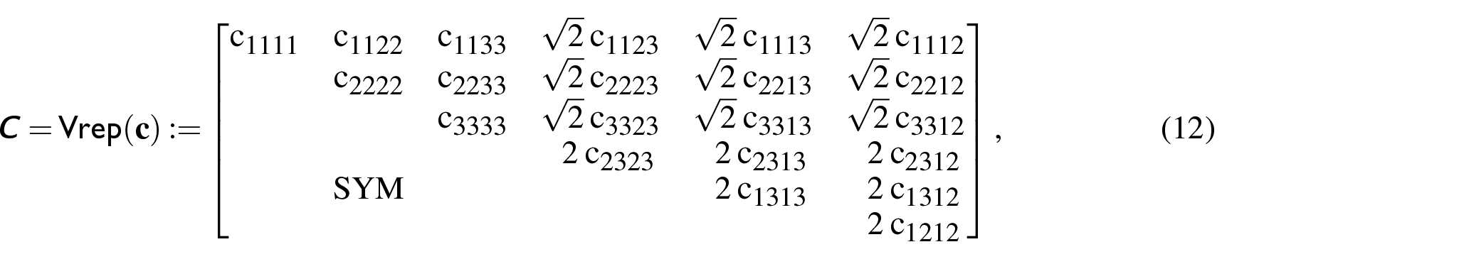
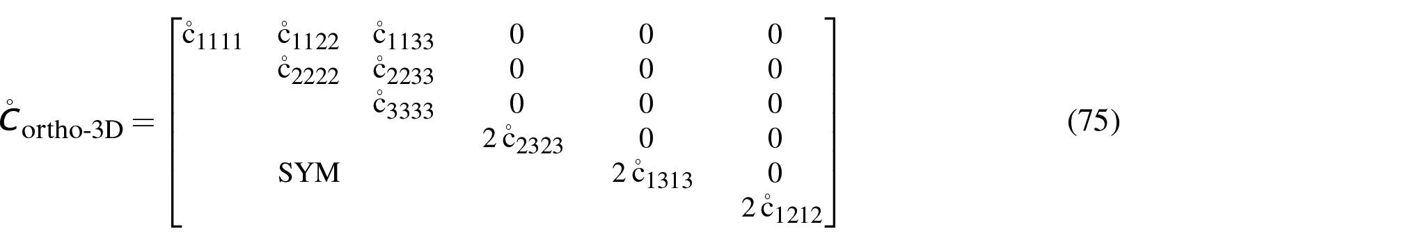
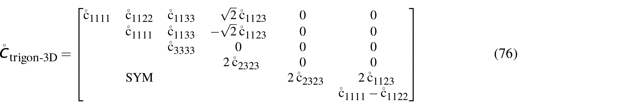
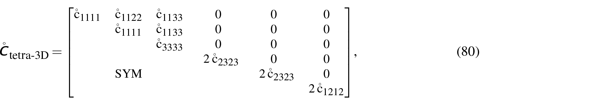
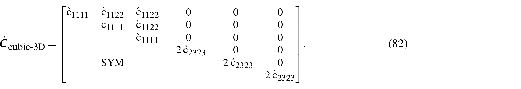
with an SPD Kelvin matrix $\mathsf{C}\in {ℒ}_s(\mathcal{T})$ , thereby establishing a linear map $\mathsf{Vrep}:\mathcal{E}\to {ℒ}_s(\mathcal{T})$ , $\mathsf{C}=\mathsf{Vrep}(\mathbf{c})$ . In terms of the components of $\mathbf{c}=(c_{i_1{i}_2{i}_3{i}_4})$ , in 3D the Kelvin matrix C and thus the map $\mathsf{Vrep}$ is given by

$$\mathsf{C}=\mathsf{Vrep}(\mathbf{c}):=\left[\begin{array}{cccccc}\hfill {\mathrm{c}}_{1111}\hfill & \hfill {\mathrm{c}}_{1122}\hfill & \hfill {\mathrm{c}}_{1133}\hfill & \hfill \sqrt{2}{\mathrm{c}}_{1123}\hfill & \hfill \sqrt{2}{\mathrm{c}}_{1113}\hfill & \hfill \sqrt{2}{\mathrm{c}}_{1112}\hfill \\ \hfill & \hfill {\mathrm{c}}_{2222}\hfill & \hfill {\mathrm{c}}_{2233}\hfill & \hfill \sqrt{2}{\mathrm{c}}_{2223}\hfill & \hfill \sqrt{2}{\mathrm{c}}_{2213}\hfill & \hfill \sqrt{2}{\mathrm{c}}_{2212}\hfill \\ \hfill & \hfill & \hfill {\mathrm{c}}_{3333}\hfill & \hfill \sqrt{2}{\mathrm{c}}_{3323}\hfill & \hfill \sqrt{2}{\mathrm{c}}_{3313}\hfill & \hfill \sqrt{2}{\mathrm{c}}_{3312}\hfill \\ \hfill & \hfill & \hfill & \hfill 2{\mathrm{c}}_{2323}\hfill & \hfill 2{\mathrm{c}}_{2313}\hfill & \hfill 2{\mathrm{c}}_{2312}\hfill \\ \hfill & \hfill \mathrm{SYM}\hfill & \hfill & \hfill & \hfill 2{\mathrm{c}}_{1313}\hfill & \hfill 2{\mathrm{c}}_{1312}\hfill \\ \hfill & \hfill & \hfill & \hfill & \hfill & \hfill 2{\mathrm{c}}_{1212}\hfill \end{array}\right],$$

(12)

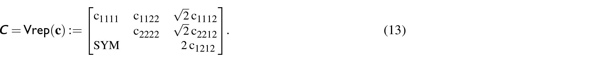
while in 2D one obtains

$$\mathsf{C}=\mathsf{Vrep}(\mathbf{c}):=\left[\begin{array}{ccc}\hfill {\mathrm{c}}_{1111}\hfill & \hfill {\mathrm{c}}_{1122}\hfill & \hfill \sqrt{2}{\mathrm{c}}_{1112}\hfill \\ \hfill & \hfill {\mathrm{c}}_{2222}\hfill & \hfill \sqrt{2}{\mathrm{c}}_{2212}\hfill \\ \hfill \mathrm{SYM}\hfill & \hfill & \hfill 2{\mathrm{c}}_{1212}\hfill \end{array}\right].$$

(13)

2.3. Group reduction and local spectral decomposition

The elasticity class [12,13,35,68,69] of the material or the elasticity tensor $\mathbf{c}\in \mathcal{E}$ [11,67] is determined by rotating the coordinate system $\hat{\mathit{x}}=\mathit{Q}\mathit{x}$ , $\mathit{Q}\in \mathrm{O}(\mathcal{V})$ in such a way as to reduce the number of constants in the fourth-order elasticity tensor $\hat{\mathbf{c}}=\mathit{Q}\star \mathbf{c}\in \mathcal{E}$ by introducing as many zeros as possible. The tensor in this form then turns out to be invariant under a whole subgroup of rotations ${\mathfrak{S}}_{\mathbf{c}}\subseteq \mathrm{O}(\mathcal{V})$ , which is called the symmetry or invariance group of the material resp. elasticity tensor. For simplicity and without loss of generality, and as more is not needed in our modelling approach, we restrict ourselves here to proper rotations, i.e., the subgroup $\mathrm{SO}(\mathcal{V})\subset \mathrm{O}(\mathcal{V})$ of special orthogonal matrices, i.e., orthogonal matrices Q with $\det \mathit{Q}=1$ . The symmetry or invariance group of a tensor will therefore in the following also be only considered as a subgroup of $\mathrm{SO}(\mathcal{V})$ .

2.3.1. Transformations of the Kelvin matrix

As just mentioned, a rotation $\mathit{Q}\in \mathrm{SO}(\mathcal{V})$ of the coordinate system in $\mathcal{V}$ induces a transformation of the stress and strain tensors [32,120] and on the fourth-order elasticity tensor $\hat{\mathbf{c}}=\mathit{Q}\star \mathbf{c}$ , as described for the general case in equation (4).

In this context, it is important to note that the linear map $\mathsf{vrep}:\mathcal{S}\to \mathcal{T}$ defined in the preceding Section 2.2 in equations (7) and (8) in 3D, and in equations (9) and (10) in 2D, is actually unitary, i.e., it preserves inner products; in fact, this is here the advantage of the Kelvin notation over the better known Voigt notation. This also means that for a rotation $\mathit{Q}\in \mathrm{SO}(\mathcal{V})$ in physical space, which one may recall preserves the inner product in $\mathcal{V}$ , there is a one-to-one correspondence $\mathsf{Trep}:\mathrm{SO}(\mathcal{V})\to \mathrm{SO}(\mathcal{T})$ [32,120] to a rotation $\mathsf{Q}=\mathsf{Trep}(\mathit{Q})\in \mathrm{SO}(\mathcal{T})$ , which in turn preserves the inner product in $\mathcal{T}$ . Concretely, this means that when $\hat{\mathit{\sigma }}=\mathit{Q}\star \mathit{\sigma }=\mathit{Q}\mathit{\sigma }{\mathit{Q}}^{\mathsf{T}}$ and $\hat{\mathit{\epsilon }}=\mathit{Q}\star \mathit{\epsilon }=\mathit{Q}\mathit{\epsilon }{\mathit{Q}}^{\mathsf{T}}$ , and

$$\mathsf{s}=\mathsf{vrep}(\mathit{\sigma }),\mathsf{e}=\mathsf{vrep}(\mathit{\epsilon }),\mathsf{ŝ}=\mathsf{vrep}(\hat{\mathit{\sigma }}),\mathsf{ê}=\mathsf{vrep}(\hat{\mathit{\epsilon }}),\mathrm{then}\mathsf{ê}=\mathsf{Q}\mathsf{e},\mathsf{ŝ}=\mathsf{Q}\mathsf{s},$$

(14)

as well as

$$\mathit{\sigma }:\mathit{\epsilon }=\hat{\mathit{\sigma }}:\hat{\mathit{\epsilon }}={\mathsf{s}}^{\mathsf{T}}\mathsf{e}={\mathsf{ŝ}}^{\mathsf{T}}\mathsf{ê};\mathrm{and}{\mathsf{s}}^{\mathsf{T}}\mathsf{s}={\mathsf{ŝ}}^{\mathsf{T}}\mathsf{ŝ},{\mathsf{e}}^{\mathsf{T}}\mathsf{e}={\mathsf{ê}}^{\mathsf{T}}\mathsf{ê}.$$

(15)

It is not too difficult to see that $\mathsf{Trep}$ is actually an injective group homomorphism. Thus the map $\mathsf{Trep}:\mathrm{SO}(\mathcal{V})\to \mathrm{SO}(\mathcal{T})$ is a unitary representation of $\mathrm{SO}(\mathcal{V})$ on $\mathcal{T}$ , see, e.g., Fässler and Stiefel [6], Jones [7], Klapper and Hahn [121] — and the precise definition of $\mathsf{Trep}$ may be found in ‘Rotations in $\mathrm{SO}(\mathcal{T})$ ’ in Appendix 2. Hence the image of $\mathrm{SO}(\mathcal{V})$ under $\mathsf{Trep}$ , which will be denoted by $\mathrm{ST}(\mathcal{T}):=\mathrm{im}\mathsf{Trep}=\mathsf{Trep}(\mathrm{SO}(\mathcal{V}))\subseteq \mathrm{SO}(\mathcal{T})$ , is a Lie subgroup of $\mathrm{SO}(\mathcal{T})$ .

As is well known, e.g., see ‘Rotations in $\mathrm{SO}(\mathcal{T})$ ’ in Appendix 2, the Lie algebra of a Lie group is the tangent vector space at the identity, and it has usually the same notation as the Lie group, but with small Fraktur letters; i.e., $\mathfrak{s}\mathfrak{o}(\mathcal{V})$ is the Lie algebra of $\mathrm{SO}(\mathcal{V})$ . The Lie algebra of $\mathrm{ST}(\mathcal{T})$ is denoted by $\mathfrak{s}\mathfrak{t}(\mathcal{T})$ . The dimension of $\mathrm{ST}(\mathcal{T})=\mathsf{Trep}(\mathrm{SO}(\mathcal{V}))$ , which is the dimension of its Lie algebra $\mathfrak{s}\mathfrak{t}(\mathcal{T})$ , is due to the injectivity of $\mathsf{Trep}$ that of $\mathrm{SO}(\mathcal{V})$ resp. $\mathfrak{s}\mathfrak{o}(\mathcal{V})$ , i.e., $\dim (\mathfrak{s}\mathfrak{o}(\mathcal{V}))=\dim (\mathfrak{s}\mathfrak{t}(\mathcal{T}))$ . The injective group homomorphism $\mathsf{Trep}:\mathrm{SO}(\mathcal{V})\to \mathrm{ST}(\mathcal{T})\subset \mathrm{SO}(\mathcal{T})$ induces an injective linear map on the corresponding Lie algebras $\mathsf{trep}:\mathfrak{s}\mathfrak{o}(\mathcal{V})\to \mathfrak{s}\mathfrak{o}(\mathcal{T})$ , such that $\mathfrak{s}\mathfrak{t}(\mathcal{T})=\mathsf{trep}(\mathfrak{s}\mathfrak{o}(\mathcal{V}))$ , details of which may also be found in ‘Rotations in $\mathrm{SO}(\mathcal{T})$ ’ in Appendix 2.

This implies that for a coordinate transform $\mathit{Q}\in \mathrm{SO}(\mathcal{V})$ , which transforms the elasticity tensor $\mathbf{c}\in \mathcal{E}$ according to equation (4) as $\hat{\mathbf{c}}=\mathit{Q}\star \mathbf{c}$ , and whose induced transformation on $\mathcal{T}$ is $\mathsf{Q}=\mathsf{Trep}(\mathit{Q})\in \mathrm{ST}(\mathcal{T})$ , the effect on the Kelvin matrix $\mathsf{C}=\mathsf{Vrep}(\mathbf{c})\in {ℒ}_s(\mathcal{T})$ is given by [32,34–36]

$$\mathsf{Ĉ}=\mathsf{Q}\mathsf{C}{\mathsf{Q}}^{\mathsf{T}}=\mathsf{Vrep}(\mathit{Q}\star \mathbf{c})=\mathsf{Vrep}(\hat{\mathbf{c}}).$$

(16)

2.3.2. Group reduction

After this preparation one may address the group reduction, [6,7] and [11–13,35,67–69]. As already indicated, one seeks a rotation $\mathit{Q}\in \mathrm{SO}(\mathcal{V})$ such that $\stackrel{°}{\mathbf{c}}=\mathit{Q}\star \mathbf{c}$ has as many zeros as possible. For the corresponding Kelvin matrix $\stackrel{°}{\mathsf{C}}=\mathsf{Vrep}(\stackrel{°}{\mathbf{c}})\in {ℒ}_s(\mathcal{T})$ this means (cf. equation (16)) that

$$\stackrel{°}{\mathsf{C}}=\mathrm{diag}({\stackrel{°}{\mathsf{C}}}_j)=\mathsf{Q}\mathsf{C}{\mathsf{Q}}^{\mathsf{T}}$$

(17)

has block diagonal form with diagonal blocks ${\stackrel{°}{\mathsf{C}}}_j$ , [6]. This $\stackrel{°}{\mathsf{C}}$ is called the group reduction of $\mathsf{C}={\mathsf{Q}}^{\mathsf{T}}\stackrel{°}{\mathsf{C}}\mathsf{Q}$ , and the blocks ${\stackrel{°}{\mathsf{C}}}_j$ on the diagonal indicate invariant subspaces of $\stackrel{°}{\mathsf{C}}\in {\mathrm{Sym}}^{+}(\mathcal{T})\subset \mathfrak{s}\mathfrak{y}\mathfrak{m}(\mathcal{T})$ . The non-diagonal minimum non-zero pattern of $\stackrel{°}{\mathsf{C}}$ is characteristic for the elasticity class, and invariant under the rotations $\mathsf{V}=\mathsf{Trep}(\mathit{V})\in {\mathfrak{S}}_{\mathsf{C}}$ with $\mathsf{V}\in {\mathfrak{S}}_{\mathbf{c}}\subseteq \mathrm{SO}(\mathcal{V})$ . In fact, the elasticity classes are commonly discussed in this group reduced form [11–13,35,67–69]. When considering random choices resp. a stochastic model for C , it may be observed that the mean or expected value may be invariant under a larger group ${\mathfrak{S}}_{\mathbf{c},m}$ for $\mathbf{c}\in \mathcal{S}$ resp. ${\mathfrak{S}}_{\mathsf{C},m}$ for $\mathsf{C}\in \mathfrak{s}\mathfrak{y}\mathfrak{m}(\mathcal{T})$ [11], i.e., ${\mathfrak{S}}_{\mathbf{c}}\subseteq {\mathfrak{S}}_{\mathbf{c},m}$ and ${\mathfrak{S}}_{\mathsf{C}}\subseteq {\mathfrak{S}}_{\mathsf{C},m}$ . Some possible choices for a mean will be investigated in Sections 3.2 and 3.3.

Observe that a completely diagonal form with a diagonal $\stackrel{°}{\mathsf{C}}$ would mean that equation (17) is an eigenvalue or spectral decomposition. But it is usually not possible to achieve a completely diagonal form just with rotations $\mathsf{Q}\in \mathrm{ST}(\mathcal{T})$ , see also Kowalczyk–Gajewska and Ostrowska–Maciejewska [41], Itin and Hehl [122], the general reason for which will be touched on now.

As already remarked in ‘Rotations in $\mathrm{SO}(\mathcal{T})$ ’ in Appendix 2, the dimension of $\mathcal{V}={\mathrm{ℝ}}^d$ is for $d>1$ smaller than that of $\mathcal{T}$ — $\dim \mathcal{V}<\dim \mathcal{T}=\dim \mathcal{S}=\dim ({ℒ}_s(\mathcal{V}))$ —which implies that the dimension of the Lie group $\mathrm{SO}(\mathcal{V})$ , is also smaller than that of the Lie group $\mathrm{SO}(\mathcal{T})$ , i.e., $\dim (\mathfrak{s}\mathfrak{o}(\mathcal{V}))<\dim (\mathfrak{s}\mathfrak{o}(\mathcal{T}))$ . This in turn means that $\mathrm{ST}(\mathcal{T})$ is a proper subgroup of the full Lie group $\mathrm{SO}(\mathcal{T})$ of proper rotations on $\mathcal{T}$ , i.e., $\mathrm{ST}(\mathcal{T})\subset \mathrm{SO}(\mathcal{T})$ . A similar relation obviously holds for its Lie algebra, $\mathfrak{s}\mathfrak{t}(\mathcal{T})\subset \mathfrak{s}\mathfrak{o}(\mathcal{T})$ and $\dim (\mathfrak{s}\mathfrak{t}(\mathcal{T}))=\dim (\mathfrak{s}\mathfrak{o}(\mathcal{V}))<\dim (\mathfrak{s}\mathfrak{o}(\mathcal{T}))$ .

2.3.3. Spectral decomposition

The group reduction just discussed commonly produces a block-diagonal matrix $\stackrel{°}{\mathsf{C}}$ . In order for $\stackrel{°}{\mathsf{C}}\in {ℒ}_s(\mathcal{T})$ in equation (17) to completely diagonalise $\mathsf{C}\in {ℒ}_s(\mathcal{T})$ in general, Q would need access to the whole group $\mathrm{SO}(\mathcal{T})$ , but one is only allowed $\mathsf{Q}\in \mathrm{ST}(\mathcal{T})\subset \mathrm{SO}(\mathcal{T})$ resulting from purely spatial rotations $\mathsf{Q}=\mathsf{Trep}(\mathit{Q})$ with $\mathit{Q}\in \mathrm{SO}(\mathcal{V})$ , which as just explained is only a subgroup. Still, equation (17) is a good start, and one can now proceed a step further by noting that $\stackrel{°}{\mathsf{C}}\in {ℒ}_s(\mathcal{T})$ is symmetric and thus has a spectral decomposition

$$\stackrel{°}{\mathsf{C}}=\mathsf{V}\mathsf{\Lambda }{\mathsf{V}}^{\mathsf{T}}$$

(18)

with $\mathsf{V}\in \mathrm{SO}(\mathcal{T})$ and $\mathsf{\Lambda }$ a diagonal matrix of eigenvalues of $\stackrel{°}{\mathsf{C}}$ . As $\stackrel{°}{\mathsf{C}}$ is block-diagonal, a similar structure will appear in $\mathsf{V}\in \mathrm{SO}(\mathcal{T})$ , in fact equation (18) are separate eigenproblems for each block ${\stackrel{°}{\mathsf{C}}}_j$ from the group decomposition equation (17), see, e.g., Fässler and Stiefel [6].

As $\mathsf{C}\in {\mathrm{Sym}}^{+}(\mathcal{T})$ is SPD, so is its rotated form $\stackrel{°}{\mathsf{C}}\in {\mathrm{Sym}}^{+}(\mathcal{T})$ , and hence $\mathsf{\Lambda }\in \mathrm{Dia}{\mathrm{g}}^{+}(\mathcal{T})\subset {\mathrm{Sym}}^{+}(\mathcal{T})$ is diagonally positive; such matrices are denoted by $\mathrm{Dia}{\mathrm{g}}^{+}(\mathcal{T})$ . $\mathsf{\Lambda }\in \mathrm{Dia}{\mathrm{g}}^{+}(\mathcal{T})$ is obviously also the matrix of eigenvalues of $\mathsf{C}\in {\mathrm{Sym}}^{+}(\mathcal{T})$ , and equating equation (17) with equation (18), one obtains

$$\mathsf{V}\mathsf{\Lambda }{\mathsf{V}}^{\mathsf{T}}=\mathsf{Q}\mathsf{C}{\mathsf{Q}}^{\mathsf{T}}\Rightarrow \mathsf{C}={\mathsf{Q}}^{\mathsf{T}}\mathsf{V}\mathsf{\Lambda }{\mathsf{V}}^{\mathsf{T}}\mathsf{Q}=\mathsf{U}\mathsf{\Lambda }{\mathsf{U}}^{\mathsf{T}},$$

(19)

where $\mathsf{V}\in \mathrm{SO}(\mathcal{T})$ and $\mathsf{Q}\in \mathrm{ST}(\mathcal{T})\subset \mathrm{SO}(\mathcal{T})$ . But $\mathrm{SO}(\mathcal{T})$ is a group, and ${\mathsf{Q}}^{\mathsf{T}}={\mathsf{Q}}^{-1}\in \mathrm{ST}(\mathcal{T})\subset \mathrm{SO}(\mathcal{T})$ , so that $\mathsf{U}:={\mathsf{Q}}^{\mathsf{T}}\mathsf{V}\in \mathrm{SO}(\mathcal{T})$ , and hence equation (19) is a spectral or eigenvalue decomposition of C ; this equation will later form the basis for its representation.

2.3.4. Group invariance

Coming back to equation (17), and recollecting equation (5), invariance under some symmetry group ${\mathfrak{S}}_{\mathbf{c}}\subseteq \mathrm{SO}(\mathcal{V})$ for the reduced elasticity tensor $\stackrel{°}{\mathbf{c}}$ means that

$$\mathrm{\forall }\mathit{W}\in {\mathfrak{S}}_{\mathbf{c}}:\mathit{W}\star \stackrel{°}{\mathbf{c}}=\stackrel{°}{\mathbf{c}}.$$

(20)

For the Kelvin matrix in the group reduced block diagonal form $\stackrel{°}{\mathsf{C}}$ with $\mathit{W}\in {\mathfrak{S}}_{\mathbf{c}}$ and its associated $\mathit{W}=\mathsf{Trep}(\mathit{W})\in {\mathfrak{S}}_{\mathsf{C}}=\mathsf{Trep}({\mathfrak{S}}_{\mathbf{c}})$ , from equation (16) this translates to $\stackrel{°}{\mathsf{C}}=\mathit{W}\stackrel{°}{\mathsf{C}}{\mathit{W}}^{\mathsf{T}}$ , and hence [6]

$$\mathrm{\forall }\mathit{W}\in {\mathfrak{S}}_{\mathsf{C}}:\stackrel{°}{\mathsf{C}}\mathit{W}=\mathit{W}\stackrel{°}{\mathsf{C}},$$

(21)

where the mapped symmetry or invariance subgroup was designated as ${\mathfrak{S}}_{\mathsf{C}}=\mathsf{Trep}({\mathfrak{S}}_{\mathbf{c}})\subset \mathrm{ST}(\mathcal{T})\subset \mathrm{SO}(\mathcal{T})$ . What equation (21) says is that $\stackrel{°}{\mathsf{C}}$ and all $\mathit{W}\in {\mathfrak{S}}_{\mathsf{C}}$ commute, i.e., they are co-axial and can all be simultaneously diagonalised with $\mathsf{V}\in \mathrm{SO}(\mathcal{T})$ , see also equation (18).

It may be noted that the equation (21) is homogeneous linear in $\stackrel{°}{\mathsf{C}}$ . As $\mathsf{C}\in {\mathrm{Sym}}^{+}(\mathcal{T})\subset \mathfrak{s}\mathfrak{y}\mathfrak{m}(\mathcal{T})$ , the equations equation (21) determine a subspace $\mathfrak{s}\mathfrak{y}\mathfrak{m}\left[{\mathfrak{S}}_{\mathsf{C}}\right]\subseteq \mathfrak{s}\mathfrak{y}\mathfrak{m}(\mathcal{T})$ in the vector space of all symmetric matrices. As already mentioned, ${\mathrm{Sym}}^{+}(\mathcal{T})$ is an open convex cone in $\mathfrak{s}\mathfrak{y}\mathfrak{m}(\mathcal{T})$ ; and thus the Kelvin matrices which are invariant under ${\mathfrak{S}}_{\mathsf{C}}$ , and hence belong to the same elasticity class, are on the intersection of said subspace $\mathfrak{s}\mathfrak{y}\mathfrak{m}\left[{\mathfrak{S}}_{\mathsf{C}}\right]$ of $\mathfrak{s}\mathfrak{y}\mathfrak{m}(\mathcal{T})$ and the cone ${\mathrm{Sym}}^{+}(\mathcal{T})$ , i.e., they all lie in the cone $\mathfrak{s}\mathfrak{y}\mathfrak{m}\left[{\mathfrak{S}}_{\mathsf{C}}\right]\cap {\mathrm{Sym}}^{+}(\mathcal{T})\subset \mathfrak{s}\mathfrak{y}\mathfrak{m}(\mathcal{T})$ .

2.4. Random tensor fields

Let $\mathcal{G}\subset {\mathrm{ℝ}}^d$ be a bounded domain in a d-dimensional Euclidean space ${\mathrm{ℝ}}^d\equiv \mathcal{V}$ (here $d=2$ or $d=3$ ) where we want to model or generate a field of elasticity tensors $\mathbf{c}(\mathit{x}),\mathit{x}\in \mathcal{G}$ . Rather than the elasticity tensor, here we want equivalently to model the corresponding Kelvin matrix $\mathsf{C}=\mathsf{Vrep}(\mathbf{c})$ . As the exact value of $\mathsf{C}(\mathit{x})$ at a location $\mathit{x}\in \mathcal{G}$ may be uncertain, either due to a highly heterogeneous material, or simply a lack of knowledge about the exact value, we assume that a probabilistic model is adopted, so that the Kelvin matrix field is modelled as a in a probability sense second-order tensor valued random field (having first and second moments), i.e., a measurable mapping

$$\mathsf{C}(\mathit{x},\omega ):\mathcal{G}\times \mathrm{\Omega }\to {\mathrm{Sym}}^{+}(\mathcal{T})$$

(22)

on a probability space $(\mathrm{\Omega },\mathfrak{F},\mathrm{\mathbb{P}})$ , where $\mathrm{\Omega }$ represents the sample space containing all outcomes $\omega \in \mathrm{\Omega }$ , $\mathfrak{F}$ is the σ-algebra of measurable subsets of $\mathrm{\Omega }$ , ℙ a probability measure, and the corresponding expectation operator is denoted by $\mathbb{E}\left(\cdot \right)$ . To avoid unnecessary clutter in the notation, the argument $\mathit{x}\in \mathcal{G}$ will be omitted, unless it is necessary for understanding. The same will often be true of the argument $\omega \in \mathrm{\Omega }$ .

2.4.1. Mean field and covariance function

The first and second-order probabilistic descriptors of such a field would be the mean field, which allows to split the field into the deterministic mean $\overline{\mathsf{C}}(\mathit{x})$ and the zero mean random part $\tilde{\mathsf{C}}(\mathit{x},\omega )$ , and the covariance function

$$\begin{array}{ccc}\hfill \overline{\mathsf{C}}(\mathit{x})& :=\mathbb{E}\left(\mathsf{C}(\mathit{x},\cdot )\right)={\int }_{\mathrm{\Omega }}\mathsf{C}(\mathit{x},\omega )\mathrm{\mathbb{P}}(\mathrm{d}\omega ),\hfill & \hfill \end{array}$$

(23)

$$\begin{array}{ccc}\hfill \tilde{\mathsf{C}}(\mathit{x},\omega )& :=\mathsf{C}(\mathit{x},\omega )-\overline{\mathsf{C}}(\mathit{x}),\hfill & \hfill \end{array}$$

(24)

$$\begin{array}{ccc}\hfill {\mathrm{cov}}_{\mathsf{C}}(\mathit{x},\mathit{y})& :=\mathbb{E}\left(\tilde{\mathsf{C}}(\mathit{x},\cdot )\otimes \tilde{\mathsf{C}}(\mathit{y},\cdot )\right).\hfill & \hfill \end{array}$$

(25)

The material symmetry-group properties are now encoded in the mean and covariance function equations (23–25), see, e.g., Malyarenko and Ostoja-Starzewski [11]. Here one may see another advantage of numerically working with the Kelvin matrix—a second-order tensor—which results in a covariance which is a fourth-order valued tensor function on $\mathcal{T}$ , although with some symmetries. In case that one would form the analogue of equation (25) for the elasticity tensor $\mathbf{c}(\mathit{x},\omega )$ , i.e.,

$${\mathrm{cov}}_{\mathbf{c}}(\mathit{x},\mathit{y})=\mathbb{E}\left(\tilde{\mathit{c}}(\mathit{x},\cdot )\otimes \tilde{\mathit{c}}(\mathit{y},\cdot )\right),$$

(26)

this would be an eighth-order tensor on $\mathcal{V}$ , although with many symmetries, i.e., a much larger object.

In both cases, this large number of covariance component functions encode simultaneously the spatial correlations and the symmetry-group invariances. Here we shall follow a different route, and, as will become clear in the following Section 3, encode the symmetry-group properties of the random Kelvin matrix in a field of n real parameters $\mathit{z}(\mathit{x},\omega )\in {\mathrm{ℝ}}^n$ and a map $\mathit{z}(\mathit{x},\omega )\mapsto \mathsf{C}(\mathit{x},\omega )$ . As will be seen later, the number of parameters is at maximum $n=\dim (\mathfrak{s}\mathfrak{o}(\mathcal{T}))+\dim (\mathfrak{d}\mathfrak{i}\mathfrak{a}\mathfrak{g}(\mathcal{T}))$ .

The first- and second-order probabilistic descriptors of these parameters then are

$$\begin{array}{ccc}\hfill \overline{\mathit{z}}(\mathit{x})& :=\mathbb{E}\left(\mathit{z}(\mathit{x},\cdot )\right)={\int }_{\mathrm{\Omega }}\mathit{z}(\mathit{x},\omega )\mathrm{\mathbb{P}}(\mathrm{d}\omega ),\hfill & \hfill \end{array}$$

(27)

$$\begin{array}{ccc}\hfill \tilde{\mathit{z}}(\mathit{x},\omega )& :=\mathit{z}(\mathit{x},\omega )-\overline{\mathit{z}}(\mathit{x}),\hfill & \hfill \end{array}$$

(28)

$$\begin{array}{ccc}\hfill {\mathrm{cov}}_{\mathit{z}}(\mathit{x},\mathit{y})& :=\mathbb{E}\left(\tilde{\mathit{z}}(\mathit{x},\cdot )\otimes \tilde{\mathit{z}}(\mathit{y},\cdot )\right),\hfill & \hfill \end{array}$$

(29)

and they then only carry the information about the spatial and probabilistic distribution. The maximum number of covariance component functions in equation (29) is thus $n^2$ , but again with the normal symmetry of a symmetric matrix, and thus only $n(n+1)∕2$ . This is actually the number of independent components in both equations (25) and (26). In addition, and more importantly, as will be shown in the following Section 3, these parameters allow one to separate the information about spatial orientation, stiffness or moduli, and eigenstrain distribution through the Lie product representation, cf. Section 3.1.

2.4.2. Spatial modelling of parameter fields

The parameters will be described in general terms in Section 3.4, and then in detail for each elasticity class in Section 4. To arrive at a spatial model for the random parameter field $\mathit{z}(\mathit{x},\omega )$ , one usually aims at a separated or tensor product representation in a sum or integral of $\tilde{\mathit{z}}(\mathit{x},\omega )$ , e.g., [116].

$$\tilde{\mathit{z}}(\mathit{x},\omega )=\sum _{\ell }{\alpha }_{\ell }{\mathit{r}}_{\ell }(\mathit{x}){\zeta }_{\ell }(\omega ),\mathrm{or}\tilde{\mathit{z}}(\mathit{x},\omega )={\int }_{\mathrm{\Xi }}\alpha (\xi )\mathit{r}(\mathit{x},\xi )\zeta (\omega ,\xi )\mathrm{d}\xi .$$

(30)

Such separated representations actually follow from fairly general methods to analyse and represent parametric objects like the fields in equation (30), where the random event ω may be regarded as the parameter, resulting in tensor-product like expressions [123,124]. Here ${\zeta }_{\ell }(\omega )$ resp. $\zeta (\omega ,\xi )$ are usually zero mean unit variance random variables, ${\mathit{r}}_{\ell }(\mathit{x})$ resp. $\mathit{r}(\mathit{x},\xi )$ are possibly normalised purely spatial functions, and ${\alpha }_{\ell }$ resp. $\alpha (\xi )$ are some scaling coefficients.

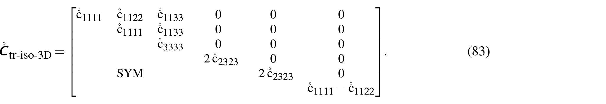
Aiming for example at a Karhunen-Loève expansion of the spatial field $\tilde{\mathit{z}}(\mathit{x},\omega )$ [116], one has to solve the Fredholm integral eigenproblem with the covariance function ${\mathrm{cov}}_{\mathit{z}}(\mathit{x},\mathit{y})$ from equation (29) as integral kernel

$${\int }_{\mathcal{G}}{\mathrm{cov}}_{\mathit{z}}(\mathit{x},\mathit{y}){\mathit{r}}_{\ell }(\mathit{y})\mathrm{d}\mathit{y}={\mu }_{\ell }{\mathit{r}}_{\ell }(\mathit{x}),$$

(31)

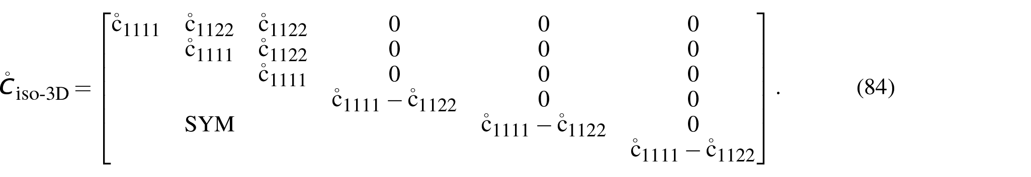
for positive eigenvalues ${\mu }_{\ell }$ and eigenvector fields ${\mathit{r}}_{\ell }(\mathit{x})\in {\mathrm{ℝ}}^n$ and $\ell \in \mathrm{\mathbb{N}}$ . Here it was tacitly assumed that the integral operator in equation (31) is self-adjoint and positive and has a discrete spectrum, which would be usually the case with a bounded domain $\mathcal{G}$ and continuous ${\mathrm{cov}}_{\mathit{z}}(\mathit{x},\mathit{y})$ for example.

It should be noted that spatial stochastic homogeneity would be evident as usual from the fact that ${\mathrm{cov}}_{\mathit{z}}(\mathit{x},\mathit{y})$ would be a function of only the difference of the arguments, $\mathit{h}:=\mathit{x}-\mathit{y}$ , say ${\mathrm{cov}}_{\mathit{z}}(\mathit{x},\mathit{y})={\mathit{K}}_{\mathit{z}}(\mathit{x}-\mathit{y})={\mathit{K}}_{\mathit{z}}(\mathit{h})$ . In that case, the eigenproblem equation (31) is a convolution equation, and it is well known how to solve those by Fourier methods, as indeed the Fourier functions are (possibly generalised) eigenfunction of the integral operator with kernel ${\mathrm{cov}}_{\mathit{z}}$ represented by equation (31). Indeed, with the eigenfunctions known, the eigenvalues are obtained by a Fourier transform—continuous or in form of a series, depending on the integral operator equation (31) and the domain $\mathcal{G}$ —of the matrix function ${\mathit{K}}_{\mathit{z}}(\mathit{h})$ above. This Fourier transform ${\hat{\mathit{K}}}_{\mathit{z}}(\mathit{k})$ , where k is the vector of wave numbers resp. spatial frequencies dual to h , is the SPD spectral matrix. Locally diagonalised for each k , it then displays the eigenvalues of the Karhunen-Loève eigenproblem equation (31). This is actually the well-known spectral description of stochastically homogeneous random fields. Further information may be found studies by Matthies [116] and in literature; therein, see also the remarks in Section 3.4. In general— non-stochastically homogeneous—case, the Karhunen-Loève eigenproblem equation (31) has to be solved numerically [125,126].

In any case, the orthonormal eigenfunctions ${\mathit{r}}_{\ell }(\mathit{x})$ determine uncorrelated mean zero unit variance random variables ${\zeta }_{\ell }(\omega )$ through the projection of $\tilde{\mathit{z}}(\mathit{x},\omega )$ , setting ${\alpha }_{\ell }=\sqrt{{\mu }_{\ell }}$ , onto the spatial eigenvector basis ${\{{\mathit{r}}_{\ell }(\mathit{x})\}}_{\ell \in \mathrm{\mathbb{N}}}$ :

$${\zeta }_{\ell }(\omega )=\frac{1}{{\alpha }_{\ell }}{\int }_{\mathcal{G}}\tilde{\mathit{z}}{(\mathit{x},\omega )}^{\mathsf{T}}{\mathit{r}}_{\ell }(\mathit{x})\mathrm{d}\mathit{x}.$$

(32)

With this one has all the ingredients for the spatial representation in equation (30), which is in this case called a Karhunen-Loève expansion, equivalent to a singular value decomposition of the random field $\tilde{\mathit{z}}(\mathit{x},\omega )$ viewed as an operator kernel [116].

As may be noted immediately, for Gaussian random fields all the uncorrelated random variables ${\zeta }_{\ell }$ in equation (32) are also Gaussian, and thus they are also independent. For modelling purposes, this is what is usually desired, a model in independent random variables. As the parameter vector field $\tilde{\mathit{z}}$ effectively models the log of the SPD tensor field, this partly explains the allure and pre-dominance of log-normal models for such SPD tensors [83]. For cases where the log-parameters $\tilde{\mathit{z}}$ are not normal, the random variables ${\zeta }_{\ell }$ are merely uncorrelated, but not independent. In this case, it is possible to express these random variables in Norbert Wiener’s polynomial chaos expansion [116,125,126] and the references therein. Thus one may represent ${\zeta }_{\ell }(\omega )$ by a series of multi-variate polynomials ${\Psi }_{\mathfrak{a}}$ — $\mathfrak{a}$ is typically a multi-index—in independent mean zero unit variance Gaussian random variables $\mathit{\xi }(\omega )=({\xi }_1(\omega ),\dots ,{\xi }_j(\omega ),\dots )$ as

$${\zeta }_{\ell }(\omega )=\sum _{\mathfrak{a}}{\beta }_{\mathfrak{a}}^{\ell }{\Psi }_{\mathfrak{a}}(\mathit{\xi }(\omega )),$$

(33)

with some coefficients ${\beta }_{\mathfrak{a}}^{\ell }$ . This then yields the field $\tilde{\mathit{z}}$ in equation (30) as a function of independent standard Gaussian variables $\mathit{\xi }(\omega )$ :

$$\tilde{\mathit{z}}(\mathit{x},\omega )=\sum _{\ell }{\alpha }_{\ell }\left(\sum _{\mathfrak{a}}{\beta }_{\mathfrak{a}}^{\ell }{\Psi }_{\mathfrak{a}}(\mathit{\xi }(\omega ))\right){\mathit{r}}_{\ell }(\mathit{x})=\sum _{\mathfrak{a}}{\Psi }_{\mathfrak{a}}(\mathit{\xi }(\omega )){\mathit{g}}_{\mathfrak{a}}(\mathit{x}),$$

(34)

where the expression ${\mathit{g}}_{\mathfrak{a}}(\mathit{x}):={\mathrm{\sum }}_{\ell }{\alpha }_{\ell }{\beta }_a^{\ell }{\mathit{r}}_{\ell }(\mathit{x})$ may be seen as the polynomial chaos expansion coefficient.

The foregoing covers the modelling aspect. To perform the reverse task, the inverse problem of conditioning [127–129], one has to change the descriptions in equations (30), (33), and (34), e.g., spatial functions ${\mathit{r}}_{\ell }(\mathit{x})$ and the random variables ${\zeta }_{\ell }(\omega )$ such that $\mathit{z}(\mathit{x},\omega )$ has the proper statistics at each $\mathit{x}\in \mathcal{G}$ . This can range from finding the SPD tensor closest to measurements [97,99,130] to conditioning the random SPD tensor field [111,131–136]. One may note that some of the filtering methods—e.g. the Gauss–Markov–Kalman filter—for Bayesian conditioning work directly on the polynomial chaos expansion coefficients ${\mathit{g}}_{\mathfrak{a}}(\mathit{x})$ in equation (34) [132–135,137–139].

3. Modelling of elasticity tensors

The main idea from the preceding Section 2.3 for the modelling approach to be discussed here is contained in the equations (17), (18) and (19), which are collected here for easy reference:

$$\stackrel{°}{\mathsf{C}}=\mathsf{Q}\mathsf{C}{\mathsf{Q}}^{\mathsf{T}},\stackrel{°}{\mathsf{C}}=\mathsf{V}\mathsf{\Lambda }{\mathsf{V}}^{\mathsf{T}}\Rightarrow \mathsf{C}={\mathsf{Q}}^{\mathsf{T}}\mathsf{V}\mathsf{\Lambda }{\mathsf{V}}^{\mathsf{T}}\mathsf{Q}=\mathsf{U}\mathsf{\Lambda }{\mathsf{U}}^{\mathsf{T}},\mathrm{with}\mathsf{U}:={\mathsf{Q}}^{\mathsf{T}}\mathsf{V}.$$

(35)

Here $\stackrel{°}{\mathsf{C}}\in {\mathrm{Sym}}^{+}(\mathcal{T})$ is the group reduced form of the Kelvin matrix $\mathsf{C}\in {\mathrm{Sym}}^{+}(\mathcal{T})$ , and $\mathsf{Q}=\mathsf{Trep}(\mathit{Q})\in \mathrm{ST}(\mathcal{T})$ with $\mathit{Q}\in \mathrm{SO}(\mathcal{V})$ , $\mathsf{V}\in \mathrm{SO}(\mathcal{T})$ and hence $\mathsf{U}\in \mathrm{SO}(\mathcal{T})$ as well, and $\mathsf{\Lambda }\in \mathrm{Dia}{\mathrm{g}}^{+}(\mathcal{T})$ .

3.1. Lie representation

Thus, given $\stackrel{°}{\mathsf{C}}$ in the form of $\mathsf{V}\mathsf{\Lambda }{\mathsf{V}}^{\mathsf{T}}$ , which means in form of an eigenstrain distribution V and eigenvalues $\mathsf{\Lambda }$ , plus an orientation $\mathit{Q}\in \mathrm{SO}(\mathcal{V})$ in space which describes the rotation from C to $\stackrel{°}{\mathsf{C}}$ , one may form $\mathsf{Q}=\mathsf{Trep}(\mathit{Q})$ and $\mathsf{U}={\mathsf{Q}}^{\mathsf{T}}\mathsf{V}$ and then generate C :

$$(\mathit{Q},\mathsf{V},\mathsf{\Lambda })\mapsto (\mathsf{Q}=\mathsf{Trep}(\mathit{Q}),\mathsf{V},\mathsf{\Lambda })\mapsto (\mathsf{U}={\mathsf{Q}}^{\mathsf{T}}\mathsf{V},\mathsf{\Lambda })\mapsto \mathsf{C}=\mathsf{U}\mathsf{\Lambda }{\mathsf{U}}^{\mathsf{T}}.$$

(36)

This is a mapping from $\mathrm{SO}(\mathcal{V})\times \mathrm{SO}(\mathcal{T})\times \mathrm{Dia}{\mathrm{g}}^{+}(\mathcal{T})$ to ${\mathrm{Sym}}^{+}(\mathcal{T})$ , resp. from $\mathrm{ST}(\mathcal{T})\times \mathrm{SO}(\mathcal{T})\times \mathrm{Dia}{\mathrm{g}}^{+}(\mathcal{T})$ to ${\mathrm{Sym}}^{+}(\mathcal{T})$

3.1.1. Lie group representation of the Kelvin matrix

The representation equation (36) will be called the Lie group representation of the Kelvin matrix $\mathsf{C}\in {\mathrm{Sym}}^{+}(\mathcal{T})$ , as $\mathit{Q}\in \mathrm{SO}(\mathcal{V})$ resp. $\mathsf{Q}\in \mathrm{ST}(\mathcal{T})$ and $\mathsf{V}\in \mathrm{SO}(\mathcal{T})$ are elements from matrix Lie groups. But the diagonal SPD matrices $\mathrm{Dia}{\mathrm{g}}^{+}(\mathcal{T})$ form a commutative or Abelian Lie group under matrix multiplication, and hence $\mathsf{\Lambda }\in \mathrm{Dia}{\mathrm{g}}^{+}(\mathcal{T})$ is also from a Lie group. The Lie representation in equation (36) is thus one on a product ${\mathsf{S}}_p$ of Lie groups [4,70–72,83], which is again a Lie group:

$${\mathsf{S}}_p:=\mathrm{ST}(\mathcal{T})\times \mathrm{SO}(\mathcal{T})\times \mathrm{Dia}{\mathrm{g}}^{+}(\mathcal{T}).$$

(37)

It should be noted here that the representation in equation (36) is not unique. What is unique is the spectrum of $\mathsf{C}\in {\mathrm{Sym}}^{+}(\mathcal{T})$ , i.e., the set of diagonal elements of $\mathsf{\Lambda }\in \mathrm{Dia}{\mathrm{g}}^{+}(\mathcal{T})$ . They could be re-ordered, inducing a re-ordering of the columns of $\mathsf{V}\in \mathrm{SO}(\mathcal{T})$ . This could be avoided by insisting on an ordering, say by size, of the diagonal elements ${\lambda }_i$ of $\mathsf{\Lambda }$ . But even more significantly, when degenerate or multiple eigenvalues occur, as is always the case for the ‘higher’ elasticity classes (cf. Section 4), those eigenvalues are associated with invariant subspaces of dimension two or higher. This makes the quest for an orthonormal eigenvector basis of such an invariant subspace—the associated columns of $\mathsf{V}\in \mathrm{SO}(\mathcal{T})$ —a matter of arbitrary choice.

As further detailed in ‘Elasticity distance’ in Appendix 1, for a general Lie group G, its Lie algebra $\mathfrak{g}$ , the tangent space at the identity, plays an important role [140–143]. Specifically, it is possible to use the Lie exponential map—for matrix Lie groups and algebras this is the usual matrix exponential— $\exp :\mathfrak{g}\to G$ to represent elements of the group G on a the free vector space $\mathfrak{g}$ ; the inverse of this map is the $\log :G\to \mathfrak{g}$ . Here we want to parametrise the product Lie group equation (37) in this way via its Lie algebra.

3.1.2. Exponential Lie algebra representation of the Kelvin matrix

The exponential and the logarithm allow one to shift the representation from the Lie group ${\mathsf{S}}_p$ in equation (37) to its Lie algebra ${\mathfrak{s}}_p$ , which is a combination of the Lie algebras of the individual factors:

$${\mathfrak{s}}_p=\mathfrak{s}\mathfrak{t}(\mathcal{T})\times \mathfrak{s}\mathfrak{o}(\mathcal{T})\times \mathfrak{d}\mathfrak{i}\mathfrak{a}\mathfrak{g}(\mathcal{T}).$$

(38)

Here $\mathfrak{d}\mathfrak{i}\mathfrak{a}\mathfrak{g}(\mathcal{T})\subset \mathfrak{s}\mathfrak{y}\mathfrak{m}(\mathcal{T})$ is the vector space of diagonal matrices, the Lie algebra of $\mathrm{Dia}{\mathrm{g}}^{+}(\mathcal{T})$ . With the exponential map, this finally yields a representation of the Kelvin matrix C on the vector space ${\mathfrak{s}}_p$ in equation (38). It allows one also to separate the effects of spatial orientation, represented by $\mathit{Q}\in \mathrm{SO}(\mathcal{V})$ , strain distribution, as represented by $\mathsf{V}\in \mathrm{SO}(\mathcal{T})$ , and stiffness, as given by $\mathsf{\Lambda }\in {\mathrm{Sym}}^{+}(\mathcal{T})$ . In Section 3.2 and ‘Elasticity distance’ in Appendix 1, this is used further to define the ‘elasticity metric’, which is used in the sequel for Fréchet means.

It should be noted that to represent $\mathbf{c}\in \mathcal{E}$ resp. $\mathsf{C}\in {\mathrm{Sym}}^{+}(\mathcal{T})$ , usually not all of $\mathrm{SO}(\mathcal{V})$ resp. $\mathrm{ST}(\mathcal{T})$ is required, as one has invariance w.r.t. rotations $\mathit{W}\in {\mathfrak{S}}_{\mathbf{c}}$ resp. $\mathit{W}=\mathsf{Trep}(\mathit{W})\in {\mathfrak{S}}_{\mathsf{C}}$ in the symmetry group of the material. We shall not introduce the group theoretic complication which might arise from a transition to factor groups here [11,51,67], and allow possibly wrapped representations, as they occur also often in circular statistics [144,145]. A similar ‘wrapping problem’ occurs in the representation of spatial rotations $\mathrm{SO}(n)$ on its Lie algebra $\mathfrak{s}\mathfrak{o}(n)$ via the exponential map, see also the remarks at the end of ‘Rotations in $\mathrm{SO}(\mathcal{V})$ in 3D and 2D’ in Appendix 2.

As is easily seen from equations (17) and (19) and the above discussion, the group invariance properties of the symmetric tensor

$$\mathsf{H}=\log \mathsf{C}=\mathsf{U}\log (\mathsf{\Lambda }){\mathsf{U}}^{\mathsf{T}}={\mathsf{Q}}^{\mathsf{T}}\mathsf{V}\log (\mathsf{\Lambda }){\mathsf{V}}^{\mathsf{T}}\mathsf{Q}\in \mathfrak{s}\mathfrak{y}\mathfrak{m}(\mathcal{T})$$

(39)

and its exponential $\mathsf{C}=\exp \mathsf{H}$ are the same, a fact which was also used by Guilleminot and Soize [109,110]. And as we are using the Lie algebra $\mathfrak{d}\mathfrak{i}\mathfrak{a}\mathfrak{g}(\mathcal{T})$ of the Lie group $\mathrm{Dia}{\mathrm{g}}^{+}(\mathcal{T})$ , we are essentially modelling $\mathsf{H}=\log \mathsf{C}$ in equation (39).

Note that one should actually apply some scaling prior to using the logarithm in equation (39), as the quantities involved may have physical dimensions. One could use in equation (39) a diagonal scaling matrix $\mathsf{D}\in \mathrm{Dia}{\mathrm{g}}^{+}(\mathcal{T})$ —often this is just a multiple of the identity, $\mathsf{D}=\alpha \mathit{I}$ for some $\alpha >0$ —of the same physical dimensions as $\mathsf{\Lambda }$ and then compute with

$$\mathsf{H}=\log \mathsf{C}=\mathsf{U}\log ({\mathsf{D}}^{-1}\mathsf{\Lambda }){\mathsf{U}}^{\mathsf{T}}={\mathsf{Q}}^{\mathsf{T}}\mathsf{V}\log ({\mathsf{D}}^{-1}\mathsf{\Lambda }){\mathsf{V}}^{\mathsf{T}}\mathsf{Q}\in \mathfrak{s}\mathfrak{y}\mathfrak{m}(\mathcal{T}).$$

(40)

Or one could use a reference matrix $\hat{\mathsf{C}}\in {\mathrm{Sym}}^{+}(\mathcal{T})$ of the same physical dimensions as C —often $\hat{\mathsf{C}}=\mathsf{D}\in \mathrm{Dia}{\mathrm{g}}^{+}(\mathcal{T})$ is a diagonal matrix, or even just a multiple of the identity $\hat{\mathsf{C}}=\alpha \mathit{I}$ as above—and define the logarithm as

$$\mathsf{H}=\log ({\hat{\mathsf{C}}}^{-1∕2}\mathsf{C}{\hat{\mathsf{C}}}^{-1∕2})\in \mathfrak{s}\mathfrak{y}\mathfrak{m}(\mathcal{T}),$$

(41)

see also, e.g., Shivanand et al. [4]. It is tacitly assumed that some such transformation to non-dimensional quantities has been carried out, so there is no need to clutter the notation with it.

Together with the exponential Rodrigues formulas in Appendix 2, this means that all the invariance constraints in the Lie group representation equation (36) may be applied on the Lie algebra level in equation (38), but a little refinement is in order here. As in the product Lie group ${\mathsf{S}}_p$ the first factor $\mathrm{ST}(\mathcal{T})\subset \mathrm{SO}(\mathcal{T})$ is contained in the second one, it is clear that in the Lie algebra ${\mathfrak{s}}_p=\mathfrak{s}\mathfrak{t}(\mathcal{T})\times \mathfrak{s}\mathfrak{o}(\mathcal{T})\times \mathfrak{d}\mathfrak{i}\mathfrak{a}\mathfrak{g}(\mathcal{T})$ one has $\mathfrak{s}\mathfrak{t}(\mathcal{T})\subset \mathfrak{s}\mathfrak{o}(\mathcal{T})$ , and so the second factor can be reduced to $\mathfrak{s}\mathfrak{t}{(\mathcal{T})}^{\perp }\subset \mathfrak{s}\mathfrak{o}(\mathcal{T})$ , the orthogonal complement of $\mathfrak{s}\mathfrak{t}(\mathcal{T})$ in $\mathfrak{s}\mathfrak{o}(\mathcal{T})$ . Hence we may use for the representation the direct sum of Lie algebras

$$\mathfrak{r}=\mathfrak{s}\mathfrak{t}(\mathcal{T})\oplus \mathfrak{s}\mathfrak{t}{(\mathcal{T})}^{\perp }\oplus \mathfrak{d}\mathfrak{i}\mathfrak{a}\mathfrak{g}(\mathcal{T}).$$

(42)

Hence in order that one may represent the Kelvin matrix later in detail in Section 4, the following general picture emerges: starting with a triple $(\mathsf{R},\mathsf{P},\mathsf{M})\in \mathfrak{r}$ one first builds the logarithm H in factored form, and then C :

$$\begin{array}{ccc}\hfill (\mathsf{R},\mathsf{P},\mathsf{M})& ⟼(\exp \mathsf{R},\exp \mathsf{P},\mathsf{M})⟼\mathsf{H}={\mathsf{Q}}^{\mathsf{T}}\mathsf{V}\mathsf{M}{\mathsf{V}}^{\mathsf{T}}\mathsf{Q}=\log \mathsf{C}\hfill & \hfill \end{array}$$

(43)

$$\begin{array}{ccc}\hfill & ⟼\mathsf{C}=\mathsf{U}\exp (\mathsf{M}){\mathsf{U}}^{\mathsf{T}}=\mathsf{U}\mathsf{\Lambda }{\mathsf{U}}^{\mathsf{T}}=\exp \mathsf{H},\hfill & \hfill \end{array}$$

(44)

where, as before, $\mathsf{Q}=\exp \mathsf{R}$ , $\mathsf{V}=\exp \mathsf{P}$ , $\mathsf{U}={\mathsf{Q}}^{\mathsf{T}}\mathsf{V}$ , and $\mathsf{\Lambda }=\exp \mathsf{M}$ ; in between one has $\mathsf{H}=\log \mathsf{C}\in \mathfrak{s}\mathfrak{y}\mathfrak{m}(\mathcal{T})$ , and finally $\mathsf{C}=\exp \mathsf{H}\in {\mathrm{Sym}}^{+}(\mathcal{T})$ . This exponential representation $\exp :\mathfrak{s}\mathfrak{y}\mathfrak{m}(\mathcal{T})\to {\mathrm{Sym}}^{+}(\mathcal{T})$ ensures positive definiteness of C .

As what we finally seek is a measurable map $\mathsf{C}:\mathcal{G}\times \mathrm{\Omega }\to {\mathrm{Sym}}^{+}(\mathcal{T})$ to give the elasticity Kelvin matrix $\mathsf{C}(\mathit{x},\omega )$ for a location $\mathit{x}\in \mathcal{G}$ and event $\omega \in \mathrm{\Omega }$ , from what was just outlined in equation (43), this will be done in several steps. One of them is to produce random tensor fields with values in $\mathfrak{r}$ in equation (42), i.e., random triples $\mathcal{G}\times \mathrm{\Omega }\to (\mathsf{R},\mathsf{P},\mathsf{M})\in \mathfrak{r}$ . From this, at each location x and event ω, the log tensor $\mathsf{H}=\log \mathsf{C}$ is built according to equation (43), and then finally $\mathsf{C}=\exp \mathsf{H}$ as just described in equation (44).

In order to put the choice of random elements into proper perspective, in the following Sections 3.2 and 3.3 some consideration on how to to choose a suitable kind of mean or expectation operator on ${\mathrm{Sym}}^{+}$ will be given, together with some requirements for such a choice. Then we can continue on how to generate random Kelvin matrices in general in Section 3.4.

3.2. Fréchet means on manifolds

As the set of SPD maps ${\mathrm{Sym}}^{+}(\mathcal{T})$ is not a flat vector space, but a manifold which can be accessed in different ways, this leads to the question of what kind of average or mean to use for elements of ${\mathrm{Sym}}^{+}(\mathcal{T})\subset \mathfrak{s}\mathfrak{y}\mathfrak{m}(\mathcal{T})$ , and this is tied to the question of how distances are measured on this set. As the ambient space $\mathfrak{s}\mathfrak{y}\mathfrak{m}(\mathcal{T})$ is a vector space, it appears at first natural to calculate averages and means as one would in a vector space, using the common arithmetic or Euclidean mean. But, as mentioned already in Section 1, it has been found that by using this kind of mean, one introduces undesirable effects [73–82]. As further described, there in Section 1 and also in Appendix 1, these are the so-called the swelling, fattening, and shrinking effects [20,70–72,82,83].

3.2.1. Variational characterisation of the mean

In this context where we want to describe shortly how to generalise the arithmetic or Euclidean mean. One may note first that the mean has a variational characterisation, cf. also ‘Fréchet mean’ in Appendix 1 and [4,16,73,82,85,90,92,94,96,146–148] for further discussion, which is the key for further generalisation. This characterisation is reproduced in Appendix 1 for better reference, see equations (86–88), and it is based on a minimisation:

$${\overline{\mathit{X}}}^{(\vartheta )}:=\arg \underset{\mathit{X}\in \mathfrak{s}\mathfrak{y}\mathfrak{m}(\mathcal{T})}{\min }{\Psi }_{\vartheta }(\mathit{X}),$$

(45)

where the X -based variance ${\Psi }_{\vartheta }(\mathit{X})$ (cf. also equation (88)) is the so-called ‘loss function’, here based on the general distance function resp. metric ϑ. In the simple case of a finite collection of items $\{{\mathit{X}}_j\}$ to be averaged this would be ${\Psi }_{\vartheta }(\mathit{X})={\mathrm{\sum }}_j{w}_j\vartheta {(\mathit{X},{\mathit{X}}_j)}^2$ , with weights $w_j\ge 0$ , ${\mathrm{\sum }}_j{w}_j=1$ . The usual arithmetic resp. Euclidean mean is obtained by use of the Euclidean distance ${\vartheta }_2$ in ${\Psi }_{\vartheta }(\mathit{X})$ , see Appendix 1. But a Euclidean distance on ${\mathrm{Sym}}^{+}(\mathcal{T})$ is not necessarily natural, and it is what seems to be responsible for the undesirable effects just mentioned. So one has to look for other distance functions ϑ, cf. also ‘Elasticity distance’ in Appendix 1, which to use in equation (45) in place of the Euclidean metric ${\vartheta }_2$ in the variational characterisation.

3.2.2. Possible alternative means

There are several possible choices, cf. ‘Elasticity distance’ in Appendix 1 and [4,16,73,82,85,90,92,94,96,146–148], as well as the references therein. The connection with Section 3.1 is as follows. It has been mentioned here before that the set of positive-definite matrices ${\mathrm{Sym}}^{+}(\mathcal{T})\subset \mathfrak{s}\mathfrak{y}\mathfrak{m}(\mathcal{T})$ is geometrically an open convex cone in $\mathfrak{s}\mathfrak{y}\mathfrak{m}(\mathcal{T})$ . Hence ${\mathrm{Sym}}^{+}(\mathcal{T})$ can be equipped with the structure of a differentiable manifold.

The representation of ${\mathrm{Sym}}^{+}(\mathcal{T})$ on the product Lie group ${\mathsf{S}}_p$ in equation (37), and via the maps equation (43) finally on the vector space ${\mathfrak{s}}_p$ in equation (38), allows one to map a Euclidean structure on the Lie algebra ${\mathfrak{s}}_p$ onto a Riemannian structure on the product Lie group ${\mathsf{S}}_p$ , each factor separately, see Appendix 1 for more details. The Riemannian structure enables the definition of geodesics—locally shortest paths—and thus allows to define a distance between two elements of each of the factor groups as the length of the shortest geodesic between those two elements.

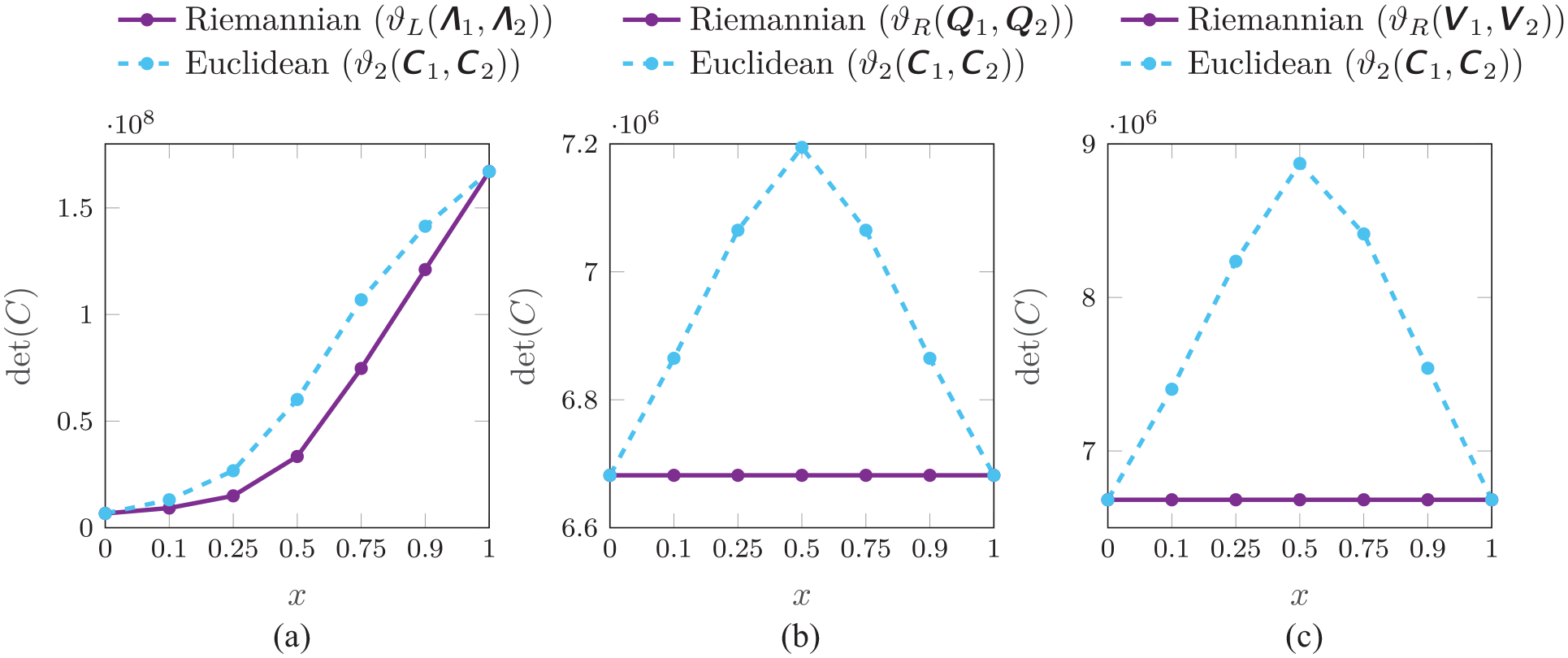
From this, one may define a product metric on the product Lie group ${\mathsf{S}}_p$ [4,70–72,80,82,83], and take this as the basis for a metric on ${\mathrm{Sym}}^{+}(\mathcal{T})$ . The product Lie group ${\mathsf{S}}_p$ used here has a finer structure than that used for ${\mathrm{Sym}}^{+}(\mathcal{V})$ by Shivanand et al. [4], or general SPD matrices by Jung et al. [70], Groisser et al. [71,72], Feragen and Fuster [82], Schwartzman [83], which only uses the spectral decomposition equation (19), which would correspond to a representation on only $\mathrm{SO}(\mathcal{T})\times \mathrm{Dia}{\mathrm{g}}^{+}(\mathcal{T})$ . Here we want to use this finer structure given by the representation in equation (36), which includes the invariance resp. symmetry group reduction, in the definition of a new metric, which is explained in detail in ‘Elasticity distance’ in Appendix 1. It is proposed to call this metric the ‘elasticity metric’ or ‘elasticity distance’ ${\vartheta }_E$ in equation (95). It allows a fine control to measure differences in spatial orientation $\mathsf{Q}\in \mathrm{ST}(\mathcal{T})$ in equation (36), differences in strain distributors $\mathsf{V}\in \mathrm{SO}(\mathcal{T})$ , and differences in Kelvin moduli $\mathsf{\Lambda }\in \mathrm{Dia}{\mathrm{g}}^{+}(\mathcal{T})$ , and combine them with different weights (cf. ‘Elasticity distance’ in Appendix 1).

It is based on the product distance on ${\mathsf{S}}_p$ (see equation (93) in ‘Elasticity distance’ in Appendix 1). For two elements ${\mathsf{C}}_1,{\mathsf{C}}_2\in {\mathrm{Sym}}^{+}(\mathcal{T})$ with representations ${\mathsf{C}}_j={\mathsf{Q}}_j^{\mathsf{T}}{\mathsf{V}}_j{\mathsf{\Lambda }}_j{\mathsf{V}}_j^{\mathsf{T}}{\mathsf{Q}}_j$ , $j=1,2$ based on $({\mathsf{R}}_j,{\mathsf{P}}_j,{\mathsf{M}}_j)\in \mathfrak{r}$ as in equation (43), the squared product distance ${\tilde{\vartheta }}_E^2$ is given by

$${\tilde{\vartheta }}_E{({\mathsf{C}}_1,{\mathsf{C}}_2)}^2={\vartheta }_L{({\mathsf{\Lambda }}_1,{\mathsf{\Lambda }}_2)}^2+c_{\mathcal{V}}{\vartheta }_R{({\mathit{Q}}_1,{\mathit{Q}}_2)}^2+c_{\mathcal{T}}{\vartheta }_R{({\mathsf{V}}_1,{\mathsf{V}}_2)}^2,$$

(46)

with two positive tuning constants $c_{\mathcal{V}},c_{\mathcal{T}}$ . The distances on the component Lie groups are: for the rotation groups the standard Riemannian metric (cf. equation (89)) ${\vartheta }_R({\mathit{Q}}_1,{\mathit{Q}}_2)={\parallel \log ({\mathit{Q}}_1{\mathit{Q}}_2^{\mathsf{T}})\parallel }_F$ with ${\mathit{Q}}_j\in \mathrm{SO}(\mathcal{V})$ , and completely analogous also for ${\vartheta }_R({\mathsf{V}}_1,{\mathsf{V}}_2)$ with ${\mathsf{V}}_j\in \mathrm{SO}(\mathcal{T})$ ; and for $\mathrm{Dia}{\mathrm{g}}^{+}(\mathcal{T})$ also the logarithmic Riemannian metric (cf. equation (90)) ${\vartheta }_L({\mathsf{\Lambda }}_1,{\mathsf{\Lambda }}_2):={\parallel \log {\mathsf{\Lambda }}_1-\log {\mathsf{\Lambda }}_2\parallel }_F={\parallel {\mathsf{M}}_1-{\mathsf{M}}_2\parallel }_F$ . IN addition, one has now to worry about the non-uniqueness of the product representation, to obtain from ${\tilde{\vartheta }}_E$ in equation (46) the final elasticity distance ${\vartheta }_E$ in equation (95). Here, as shown in ‘Elasticity distance’ in Appendix 1, one minimises over all possible Lie product group representations $\mathsf{C}={\mathsf{Q}}^{\mathsf{T}}\mathsf{V}\mathsf{\Lambda }{\mathsf{V}}^{\mathsf{T}}\mathsf{Q}$ , and, as the geodesic is only locally a shortest path, over all ‘intermediate stops’; but for small variations equation (46) is all what is needed.

To recap quickly Appendix 1 here, with this elasticity metric one may go back to equation (45), employing the variational characterisation with metric ϑ, and replace the Euclidean metric $\vartheta ={\vartheta }_2$ with the elasticity metric $\vartheta ={\vartheta }_E$ mentioned in equation (95). At the end of Appendix 1, an elasticity Fréchet mean or expected value ${\mathbb{E}}_{{\vartheta }_E}$ is thus defined in equation (96) for a random elasticity tensor, utilising as loss function the $\overline{\mathsf{C}}$ -based variance ${\Psi }_{{\vartheta }_E}(\overline{\mathsf{C}})$ in equation (97), which is based on the elasticity metric ${\vartheta }_E$ in equation (94).

3.3. Requirements for representation and mean

While the introduction of a new metric and mean where motivated in the preceding Section 3.2 by geometrical considerations, it might be actually worthwhile to consider what one may require from a metric for elasticity tensors resp. Kelvin matrices, and even for any kind of numerical representation in general.

As the goal is to be able to define, model, and represent random tensor fields $\mathsf{C}(\mathit{x},\omega )$ on some spatial domain $\mathcal{G}\subset {\mathrm{ℝ}}^d$ , $d=2$ or $d=3$ with typical point $\mathit{x}\in \mathcal{G}$ , and $\omega \in \mathrm{\Omega }$ an event in some appropriate probability space $(\mathrm{\Omega },\mathfrak{F},\mathrm{\mathbb{P}})$ with σ-algebra $\mathfrak{F}$ and probability measure ℙ, i.e., a measurable map $\mathsf{C}:\mathcal{G}\times \mathrm{\Omega }\to {\mathrm{Sym}}^{+}(\mathcal{T})$ , here we formulate some requirements which in our view have to be satisfied for the modelling, so that the random tensor field $\mathsf{C}(\mathit{x},\omega )$ is usable in, e.g., stochastic FEM calculations and uncertainty quantification (e.g. Matthies [116], Soize [149] and the references therein). See also Shivanand et al. [4] for similar remarks regarding second-order SPD random tensor fields.

3.3.1. Representation requirements

The requirements we suggest should be met is that at almost all points $\mathit{x}\in \mathcal{G}$ and realisations $\omega \in \mathrm{\Omega }$ ,

1. even under numerical approximations like truncation of series resp. numerical quadrature, the tensor $\mathsf{C}(\mathit{x},\omega )$ has to be SPD, i.e., $\mathsf{C}(\mathit{x},\omega )=\mathsf{C}{(\mathit{x},\omega )}^{\mathsf{T}}\in \mathfrak{s}\mathfrak{y}\mathfrak{m}(\mathcal{T})$ , and for all $\mathit{X}\ne \mathit{0}\in \mathcal{T}:{\mathit{X}}^{\mathsf{T}}\mathsf{C}(\mathit{x},\omega )\mathit{X}>0$;

2. the tensor $\mathsf{C}(\mathit{x},\omega )$ has to be invariant under some group of transformations ${\mathfrak{S}}_{\mathsf{C}}\subseteq \mathrm{ST}(\mathcal{T})$ , the invariance or symmetry class of each realisation;

3. the mean ${\overline{\mathsf{C}}}^{({\vartheta }_D)}(\mathit{x}):={\mathbb{E}}_{{\vartheta }_D}(\mathsf{C}(\mathit{x},\cdot ))\in {\mathrm{Sym}}^{+}(\mathcal{T})$ based on some desirable metric ${\vartheta }_D$ has to be invariant under a possibly larger group of transformations ${\mathfrak{S}}_{\mathsf{C},m}$ , with $\mathrm{ST}(\mathcal{T})\supseteq {\mathfrak{S}}_{\mathbf{c},m}\supset {\mathfrak{S}}_{\mathsf{C}}$ , the invariance or symmetry class of the mean.

The first item is a necessity in order to be able to successfully calculate with the tensor field $\mathsf{C}(\mathit{x},\omega )$ . The second item makes sure that each realisation has the proper spatial invariance resp. symmetry or elasticity class. The third item allows to control the elasticity class of the mean resp. expected value. For the most part, the concern here is the analysis, modelling, and representation of $\mathsf{C}(\mathit{x},\omega )$ at one point $\mathit{x}\in \mathcal{G}$ and sample $\omega \in \mathrm{\Omega }$ , so that for the sake of brevity these arguments will be dropped in the sequel, just as they have been in most of the description above, up to the point in Section 3.4 when spatial random fields will finally be considered.

3.3.2. Desiderata for a Fréchet mean

Turning now to the mean and metric addressed in the third item above, first note that a change of physical units or to non-dimensional quantities is a diagonal scaling like equation (40), and the mean should scale the same way, i.e., first scaling and the averaging should give the same result as first averaging and then scaling. Second, a change of coordinate system by some $\mathsf{Q}=\mathsf{Trep}(\mathit{Q})\in \mathrm{ST}(\mathcal{T})$ for any $\mathit{Q}\in \mathrm{SO}(\mathcal{V})$ should affect the same change in the mean, i.e., commutativity of averaging and coordinate transform. And finally, one may note that Hooke’s law—in vector notation in equation (129)—can just as well be formulated in terms of compliances, i.e.,

$$\mathsf{e}={\mathsf{C}}^{-1}\mathit{s}=\mathit{S}\mathit{s};\mathrm{with}\mathrm{compliance}\mathit{S}={\mathsf{C}}^{-1}.$$

(47)

Hence it seems desirable to require the ‘mean material law’ to be independent of the arbitrariness of formulating the material law, e.g., equation (129) or equation (47), and therefore demand an appropriate invariance under inversion, i.e., averaging and then inverting should give the same result as first inverting and then averaging. In simplest terms, given n Kelvin matrices ${\{{\mathsf{C}}_j\}}_{j=1}^n\subset {\mathrm{Sym}}^{+}(\mathcal{T})$ , let ${\overline{{\mathsf{C}}_j}}^{({\vartheta }_D)}$ denote their Fréchet mean based on some desirable distance ${\vartheta }_D$ , cf. Appendix 1, and let $\mathsf{Q}=\mathsf{Trep}(\mathit{Q})\in \mathrm{ST}(\mathcal{T})$ , $\mathit{Q}\in \mathrm{SO}(\mathcal{V})$ be an arbitrary spatially induced rotation. The requirements for the mean then are:

1. invariance under scaling: $\mathrm{\forall }\alpha >0$ : ${\overline{(\alpha {\mathsf{C}}_j)}}^{({\vartheta }_D)}=\alpha {\overline{{\mathsf{C}}_j}}^{({\vartheta }_D)}$ ;

2. invariance under orthogonal transformations: ${\overline{(\mathsf{Q}{\mathsf{C}}_j{\mathsf{Q}}^{\mathsf{T}})}}^{({\vartheta }_D)}=\mathsf{Q}{\overline{{\mathsf{C}}_j}}^{({\vartheta }_D)}{\mathsf{Q}}^{\mathsf{T}}$ ;

3. invariance under inversion: let ${\{{\mathit{S}}_j={\mathsf{C}}_j^{-1}\}}_{j=1}^n\subset {\mathrm{Sym}}^{+}(\mathcal{T})$ with mean ${\overline{{\mathit{S}}_j}}^{({\vartheta }_D)}$ be the inverses to the Kelvin matrices $\{{\mathsf{C}}_j\}$ , it should hold that ${\overline{{\mathit{S}}_j}}^{({\vartheta }_D)}={({\overline{{\mathsf{C}}_j}}^{({\vartheta }_D)})}^{-1}$ .

3.3.3. Desiderata for a metric to define a Fréchet mean

When looking at the variational definition of the Fréchet mean equation (45), but with another metric ${\vartheta }_D$ in place of the Euclidean metric, or the more general formulas in Appendix 1, it is quite obvious that the Fréchet mean inherits the required properties from the underlying metric ${\vartheta }_D$ on ${\mathrm{Sym}}^{+}(\mathcal{T})$ . The requirements for a desired metric ${\vartheta }_D$ , and hence for a Fréchet mean based on it, are thus to satisfy for all ${\mathsf{C}}_1,{\mathsf{C}}_2\in {\mathrm{Sym}}^{+}(\mathcal{T}),\alpha >0$ , and all $\mathsf{Q}\in \mathrm{ST}(\mathcal{T})$ :

1. quasi-invariance under scaling: ${\vartheta }_D(\alpha {\mathsf{C}}_1,\alpha {\mathsf{C}}_2)=f(\alpha ){\vartheta }_D({\mathsf{C}}_1,{\mathsf{C}}_2)$ ,

   with a monotone $f(\alpha )>0$ ;

2. invariance under orthogonal transformations: ${\vartheta }_D(\mathsf{Q}{\mathsf{C}}_1{\mathsf{Q}}^{\mathsf{T}},\mathsf{Q}{\mathsf{C}}_2{\mathsf{Q}}^{\mathsf{T}})={\vartheta }_D({\mathsf{C}}_1,{\mathsf{C}}_2)$ ;

3. invariance under inversion: ${\vartheta }_D({\mathsf{C}}_1^{-1},{\mathsf{C}}_2^{-1})={\vartheta }_D({\mathsf{C}}_1,{\mathsf{C}}_2)$ ;

The Euclidean distance ${\vartheta }_2$ satisfies only the first two items, and so the arithmetic or Euclidean mean only satisfies the first two requirements for means. The elasticity metric ${\vartheta }_E$ proposed here, see Appendix 1, satisfies all three requirements, and so does the associated mean. There are some other metrics which satisfy all three requirements, see the discussion by Shivanand et al. [4], Feragen and Fuster [82], but the elasticity metric seems to deal particularly well with the afore mentioned swelling, fattening, and shrinking effects.

3.4. Generation of random Kelvin matrices

At first assume that $\mathit{x}\in \mathcal{G}$ is fixed, i.e., consider the generation of random Kelvin matrices at one location. The spatial modelling will be described later, so the argument x will be suppressed. Similarly to the situation in Section 3.1 when introducing $\mathsf{H}=\log \mathsf{C}$ , where a ‘reference matrix’ $\hat{\mathsf{C}}\in {\mathrm{Sym}}^{+}(\mathcal{T})$ was used in equation (41), this concept is useful also here. One may actually think of the reference matrix $\hat{\mathsf{C}}$ as an appropriate mean or expected value. It will be pointed out under what conditions this holds. Start with the Lie product group decomposition of the deterministic reference matrix $\hat{\mathsf{C}}$ as in equation (36):

$$\begin{array}{ccc}\hfill \hat{\mathsf{C}}& ={\mathsf{Q}}_0^{\mathsf{T}}{\mathsf{V}}_0{\mathsf{\Lambda }}_0{\mathsf{V}}_0^{\mathsf{T}}{\mathsf{Q}}_0,\mathrm{with}({\mathsf{Q}}_0,{\mathsf{V}}_0)=(\exp {\mathsf{R}}_0,\exp {\mathsf{P}}_0),\hfill & \hfill \end{array}$$

(48)

$$\begin{array}{ccc}\hfill \mathfrak{r}\ni ({\mathsf{R}}_0,{\mathsf{P}}_0,{\mathsf{M}}_0)& \mapsto ({\mathsf{Q}}_0,{\mathsf{V}}_0,{\mathsf{M}}_0)\mapsto \hat{\mathsf{H}}:={\mathsf{Q}}_0^{\mathsf{T}}{\mathsf{V}}_0{\mathsf{M}}_0{\mathsf{V}}_0^{\mathsf{T}}{\mathsf{Q}}_0=\log \hat{\mathsf{C}}\in \mathfrak{s}\mathfrak{y}\mathfrak{m}(\mathcal{T});\hfill & \hfill \end{array}$$

(49)

from where $\hat{\mathsf{C}}=\exp \hat{\mathsf{H}}\in {\mathrm{Sym}}^{+}(\mathcal{T})$ can be recovered as in equation (44). Here one can then choose an elasticity invariance class according what is appropriate for the mean as indicated in Section 2.3, i.e., invariance under ${\mathfrak{S}}_{\mathbf{c},m}$ resp. ${\mathfrak{S}}_{\mathsf{C},m}$ .

How to pick a specific elasticity invariance class either for the mean—i.e., ${\mathfrak{S}}_{\mathbf{c},m}$ resp. ${\mathfrak{S}}_{\mathsf{C},m}$ —or for the random part—i.e., ${\mathfrak{S}}_{\mathbf{c}}$ resp. ${\mathfrak{S}}_{\mathsf{C}}$ —will be given in detail for each class in the next Section 4.

As a second step, in equation (44) each component $(\mathsf{Q},\mathsf{V},\mathsf{\Lambda })\in {\mathsf{S}}_p$ is written as a product

$$\begin{array}{ccccc}\hfill \mathsf{Q}(\omega )& ={\mathsf{Q}}_1(\omega ){\mathsf{Q}}_0,\hfill & \hfill {\mathsf{Q}}_1(\omega )& =\exp (\theta (\omega ){\mathsf{R}}_1(\omega ));\hfill & \hfill \end{array}$$

(50)

$$\begin{array}{ccccc}\hfill \mathsf{V}(\omega )& ={\mathsf{V}}_1(\omega ){\mathsf{V}}_0,\hfill & \hfill {\mathsf{V}}_1(\omega )& =\exp ({\mathsf{P}}_1(\omega ));\hfill & \hfill \end{array}$$

(51)

$$\begin{array}{ccccc}\hfill \mathsf{\Lambda }(\omega )& ={\mathsf{\Lambda }}_1(\omega ){\mathsf{\Lambda }}_0,\hfill & \hfill {\mathsf{\Lambda }}_1(\omega )& =\exp ({\mathsf{M}}_1(\omega )),\hfill & \hfill \end{array}$$

(52)

computed from random elements $(\theta (\omega ){\mathsf{R}}_1(\omega ),{\mathsf{P}}_1(\omega ),{\mathsf{M}}_1(\omega ))\in \mathfrak{r}$ . The random variable equivalent to equation (36) resp. equations (43–44) then is

$$\begin{array}{cc}\hfill & \mathsf{C}(\omega )={\mathsf{Q}}^{\mathsf{T}}(\omega )\mathsf{V}(\omega )\mathsf{\Lambda }(\omega ){\mathsf{V}}^{\mathsf{T}}(\omega )\mathsf{Q}(\omega )\hfill \\ \hfill & ={({\mathsf{Q}}_1(\omega ){\mathsf{Q}}_0)}^{\mathsf{T}}({\mathsf{V}}_1(\omega ){\mathsf{V}}_0)({\mathsf{\Lambda }}_0{\mathsf{\Lambda }}_1(\omega )){({\mathsf{V}}_1(\omega ){\mathsf{V}}_0)}^{\mathsf{T}}({\mathsf{Q}}_1(\omega ){\mathsf{Q}}_0),\hfill & \hfill \end{array}$$

(53)

where ${\mathsf{Q}}_0=\mathsf{Trep}({\mathit{Q}}_0)\in \mathrm{ST}(\mathcal{T})$ and ${\mathsf{Q}}_1(\omega )=\mathsf{Trep}({\mathit{Q}}_1(\omega ))\in \mathrm{ST}(\mathcal{T})$ originate from spatial rotations ${\mathsf{Q}}_0,{\mathsf{Q}}_1(\omega )\in \mathrm{SO}(\mathcal{V})$ .

3.4.1. Random rotations in physical space $\mathcal{V}$

The purpose of the rotation in equation (50), $\mathsf{Q}(\omega )=\mathsf{Trep}(\mathit{Q})\in \mathrm{ST}(\mathcal{T})$ , resulting from a spatial rotation $\mathit{Q}\in \mathrm{SO}(\mathcal{V})$ , is to transforms the desired final $\mathsf{C}\in {\mathrm{Sym}}^{+}(\mathcal{T})$ to the special form $\stackrel{°}{\mathsf{C}}\in {\mathrm{Sym}}^{+}(\mathcal{T})$ —that is why in equation (53) its inverse ${\mathsf{Q}}^{-1}(\omega )={\mathsf{Q}}^{\mathsf{T}}(\omega )$ is used for the back-transformation. The special forms to be addressed below for each elasticity class have at least one distinguished rotation axis—except for tri-clinic material, which has none, and isotropic material, which does not need a spatial rotation—which as is usual taken to be the three-axis. IN addition, there may be other distinguished rotation axes in the plane orthogonal to the three-axis, i.e., the 1-2-plane. In $\mathrm{O}(\mathcal{V})$ there also would be reflections, but as here we confine ourselves to proper rotations $\mathit{Q}\in \mathrm{SO}(\mathcal{V})$ , reflections are not considered any further.

As recalled in ‘Rotations in $\mathrm{SO}(\mathcal{V})$ in 3D and 2D’ in Appendix 2, a rotation $\mathit{Q}\in \mathrm{SO}(\mathcal{V})$ can be represented by a normalised skew matrix $\mathit{R}\in \mathfrak{s}\mathfrak{o}(\mathcal{V})$ and a rotation angle θ through the exponential map given by the Rodrigues formulas, equation (104) in 3D and equation (107) in 2D.

In 2D the skew matrix R is constant, cf. equation (106), whereas in 3D it is conveniently specified by a vector $\mathit{q}\in {\mathrm{ℝ}}^3,\mathit{q}=\theta \mathit{r}$ . Here r is a unit vector, and the length of q is equal to the absolute value of θ, and from that one obtains $\mathit{R}=\mathsf{skw}(\mathit{r})$ (cf. equation (103)).

In 2D one may take the parameter $q=\theta$ (a 1D vector), and in 3D the 3D-vector $\mathit{q}\in {\mathrm{ℝ}}^3$ ( $\mathit{q}=\theta \mathit{r}$ ). Thus the deterministic part ${\mathit{Q}}_0$ of $\mathit{Q}(\omega )={\mathit{Q}}_1(\omega ){\mathit{Q}}_0$ is always described by a deterministic vector ${\mathit{q}}_0\in {\mathrm{ℝ}}^{m_Q}$ , $m_Q\le \dim \mathfrak{s}\mathfrak{o}(\mathcal{V})$ (so in 2D $\dim \mathfrak{s}\mathfrak{o}(\mathcal{V})=1$ and in 3D $\dim \mathfrak{s}\mathfrak{o}(\mathcal{V})=3$ ), and the random part ${\mathit{Q}}_1(\omega )$ through a random vector ${\mathit{q}}_1(\omega )\in {\mathrm{ℝ}}^{m_Q}$ . Finally one obtains a correspondence for equation (53),

$$\begin{array}{ccc}\hfill {\mathrm{ℝ}}^{m_Q}\ni {\mathit{q}}_0& ⟼{\mathsf{Q}}_0=\mathsf{Trep}({\mathit{Q}}_0)\in \mathrm{ST}(\mathcal{T}),\hfill & \hfill \end{array}$$

(54)

$$\begin{array}{ccc}\hfill {\mathrm{ℝ}}^{m_Q}\ni {\mathit{q}}_1(\omega )& ⟼{\mathsf{Q}}_1(\omega )=\mathsf{Trep}({\mathit{Q}}_1(\omega ))\in \mathrm{ST}(\mathcal{T}),\hfill & \hfill \end{array}$$

(55)

check ‘Rotations in $\mathrm{SO}(\mathcal{T})$ ’ in Appendix 2 for further details.

One way to think of this combined rotation—a concept which is employed also for the factors $\mathsf{V}(\omega )$ and $\mathsf{\Lambda }(\omega )$ in equation (53)—is that ${\mathsf{Q}}_0\in \mathrm{ST}(\mathcal{T})$ does the ‘main part’, i.e., it transforms the block diagonal form $\stackrel{°}{\mathsf{C}}$ into the average spatial orientation. The additional factor ${\mathsf{Q}}_1(\omega )=\mathsf{Trep}({\mathit{Q}}_1(\omega ))\in \mathrm{ST}(\mathcal{T})$ introduces a random component on top of this. This will be achieved if the expected value of this random rotation ${\mathit{Q}}_1(\omega )$ —for the ${\vartheta }_R$ -metric on $\mathrm{SO}(\mathcal{V})$ in equation (89)—is the identity. The total rotation then has mean ${\mathit{Q}}_0$ . Thus, in light of equations (54–55), one may in effect say that the random orientation can be written as $\mathsf{Q}(\omega )={\mathsf{Q}}_1({\mathit{q}}_1(\omega )){\mathsf{Q}}_0({\mathit{q}}_0)$ .

The identity $\mathit{I}=\exp (\theta \mathit{R})$ corresponds to $\theta =0$ , i.e., to $\mathit{q}=\mathit{0}$ . Thus, for a random realisation, generate a random spatial rotation vector ${\mathit{q}}_1(\omega )\in {\mathrm{ℝ}}^m$ with mean at the origin. Note that from equations (89–50) one gleans that the ${\vartheta }_R$ -distance (cf. Appendix 1) between ${\mathit{Q}}_1(\omega ){\mathit{Q}}_0$ and ${\mathit{Q}}_0$ is

$${\vartheta }_R({\mathit{Q}}_1(\omega ){\mathit{Q}}_0,{\mathit{Q}}_0)={\parallel \log ({\mathit{Q}}_1(\omega ){\mathit{Q}}_0{\mathit{Q}}_0^{-1})\parallel }_F={\parallel \log {\mathit{Q}}_1(\omega )\parallel }_F={\parallel \theta (\omega ){\mathit{R}}_1(\omega )\parallel }_F.$$

(56)

As this shows, one possibility when this will make the corresponding ${\mathit{Q}}_1(\omega )$ have mean I in the ${\vartheta }_R$ metric is when $\theta (\omega ){\mathit{R}}_1(\omega )=\mathsf{skw}({\mathit{q}}_1(\omega ))$ resp. ${\mathit{q}}_1(\omega )$ has a distribution which is symmetric about the origin. Observe that if in addition to the mean (the origin) also the variance of the vector ${\mathit{q}}_1(\omega )\in {\mathrm{ℝ}}^{m_Q}$ is specified, the maximum entropy distribution [150] for ${\mathit{q}}_1(\omega )$ is the centred normal or Gaussian distribution, which obviously is symmetric to its mean, the origin.

3.4.2. Random transformations in strain space $\mathcal{T}$

This is in many ways very similar to random rotations in physical space as just described, only that $\mathsf{V}(\omega )={\mathsf{V}}_1(\omega ){\mathsf{V}}_0$ with ${\mathsf{V}}_1(\omega )=\exp ({\mathsf{P}}_1(\omega ))$ in equation (51) is in $\mathrm{SO}(\mathcal{T})$ , and the randomness enters here in a slightly different way.

As a general spatial rotation $\mathsf{Q}=\mathsf{Trep}(\mathit{Q})\in \mathrm{ST}(\mathcal{T})\subset \mathrm{SO}(\mathcal{T})$ with $\mathit{Q}\in \mathrm{SO}(\mathcal{V})$ cannot diagonalise the Kelvin matrix C for any elasticity invariance class, a further rotation $\mathsf{V}\in \mathrm{SO}(\mathcal{T})$ in strain representer space $\mathcal{T}$ is needed for this. Thus these orthogonal ${\mathsf{V}}_0\exp {\mathsf{P}}_0,{\mathsf{V}}_1(\omega )=\exp {\mathsf{P}}_1(\omega )$ , described by ${\mathsf{P}}_0,{\mathsf{P}}_1(\omega )\in \mathfrak{s}\mathfrak{t}{(\mathcal{T})}^{\perp }\subset \mathfrak{s}\mathfrak{o}(\mathcal{T})$ , are part of the material description, i.e., the definition of the block diagonal group-reduced form of the Kelvin matrix $\stackrel{°}{\mathsf{C}}$ , as its columns specify the Kelvin eigen-strain representers resp. the eigenvectors of the elasticity matrix in the invariant subspace that was found through the reduction of the group representation. So, although it is an abstract rotation one is talking about, this is not a rotation in physical space.

One chooses again, analogous as before for the spatial rotation, a deterministic ${\mathsf{P}}_0\in \mathfrak{s}\mathfrak{t}{(\mathcal{T})}^{\perp }\subset \mathfrak{s}\mathfrak{o}(\mathcal{T})$ to define the reference or mean eigen-strain, again defined by a parameter vector ${\mathit{p}}_0\in {\mathrm{ℝ}}^{m_V}$ , where $m_V\le \dim \mathfrak{s}\mathfrak{t}{(\mathcal{T})}^{\perp }$ , and a random ${\mathsf{P}}_1(\omega )\in \mathfrak{s}\mathfrak{t}{(\mathcal{T})}^{\perp }$ , also defined by a parameter vector ${\mathit{p}}_1(\omega )\in {\mathrm{ℝ}}^{m_V}$ . As previously for the spatial rotation in equations (54–55), one obtains

$$\begin{array}{ccc}\hfill {\mathrm{ℝ}}^{m_V}\ni {\mathit{p}}_0& \mapsto {\mathsf{P}}_0=\mathsf{skw}({\mathit{p}}_0)\in \mathfrak{s}\mathfrak{o}(\mathcal{T})\mapsto {\mathsf{V}}_0=\exp {\mathit{P}}_0\in \mathrm{SO}(\mathcal{T}),\hfill & \hfill \end{array}$$

(57)

$$\begin{array}{ccc}\hfill {\mathrm{ℝ}}^{m_V}\ni {\mathit{p}}_1(\omega )& \mapsto {\mathsf{P}}_1(\omega )=\mathsf{skw}({\mathit{p}}_1(\omega ))\in \mathfrak{s}\mathfrak{o}(\mathcal{T})\mapsto {\mathsf{V}}_1(\omega )=\exp {\mathit{P}}_1(\omega )\in \mathrm{SO}(\mathcal{T}).\hfill & \hfill \end{array}$$

(58)

Thus again the final result may be written as $\mathsf{V}(\omega )={\mathsf{V}}_1({\mathit{p}}_1(\omega )){\mathsf{V}}_0({\mathit{p}}_0)$ . Details for these versions of the map ${\mathit{p}}_0\mapsto {\mathsf{V}}_0$ , as well as $\mathsf{skw}$ will be given for each elasticity class in Section 4.

In case ${\mathit{p}}_1(\omega )$ has a distribution which is symmetric about the origin, and as for spatial rotations the ${\vartheta }_R$ -distance (cf. Appendix 1) is used on the Lie product factor $\mathrm{SO}(\mathcal{T})$ , similar considerations as before show that then ${\mathsf{V}}_1(\omega )$ has the ${\vartheta }_R$ -mean equal to the identity I and thus ${\mathsf{V}}_0$ is the ${\vartheta }_R$ -mean of $\mathsf{V}(\omega )={\mathsf{V}}_0{\mathsf{V}}_1(\omega )$ . And again, in case that additionally also the variance of the vector ${\mathit{p}}_1(\omega )\in {\mathrm{ℝ}}^{m_V}$ is specified, the maximum entropy distribution [150] for ${\mathit{p}}_1(\omega )$ is the centred normal or Gaussian distribution.

3.4.3. Random Kelvin moduli

The diagonal eigenvalue matrix we want to split according to equation (52), similarly as for the spatial rotations and the rotations in strain space $\mathcal{T}$ , i.e., $\mathsf{\Lambda }(\omega )={\mathsf{\Lambda }}_1(\omega ){\mathsf{\Lambda }}_0\in \mathrm{Dia}{\mathrm{g}}^{+}(\mathcal{T})$ . One may think of ${\mathsf{\Lambda }}_0$ as the deterministic or mean part, and ${\mathsf{\Lambda }}_1(\omega )$ as random with mean equal to unity. Translating this into logarithmic space, one obtains a modelling on $\mathfrak{d}\mathfrak{i}\mathfrak{a}\mathfrak{g}(\mathcal{T})$ by taking ${\mathsf{M}}_0\in \mathfrak{d}\mathfrak{i}\mathfrak{a}\mathfrak{g}(\mathcal{T})$ as fixed such that ${\mathsf{\Lambda }}_0=\exp {\mathsf{M}}_0$ and ${\mathsf{M}}_1(\omega )\in \mathfrak{d}\mathfrak{i}\mathfrak{a}\mathfrak{g}(\mathcal{T})$ as a zero mean random part such that

$$\mathsf{\Lambda }(\omega )={\mathsf{\Lambda }}_1(\omega ){\mathsf{\Lambda }}_0=(\exp {\mathsf{M}}_1(\omega ))(\exp {\mathsf{M}}_0)=\exp ({\mathsf{M}}_1(\omega )+{\mathsf{M}}_0),$$

(59)

the last equality being true as $\mathrm{Dia}{\mathrm{g}}^{+}(\mathcal{T})$ is an Abelian Lie group, and therefore ${\mathsf{\Lambda }}_0$ and ${\mathsf{\Lambda }}_1$ commute.

One may point out that in case the distribution of ${\mathsf{M}}_1(\omega )$ is symmetric to the origin, then the expected value of ${\mathsf{\Lambda }}_1(\omega )$ according to the logarithmic distance ${\vartheta }_L$ (see equation (90) in Appendix 1) will be the unit matrix I . And additionally it may be observed that the maximum entropy distribution for given mean and variance on ${\mathsf{M}}_1(\omega )$ is the centred the Gaussian or normal distribution.

To obtain a concise representation in real parameters, one chooses a deterministic vector ${\mathit{\mu }}_0=[{\mu }_{0,1},\dots ,{\mu }_{0,m_{\mathrm{\Lambda }}}]\in {\mathrm{ℝ}}^{m_{\mathrm{\Lambda }}}$ , where $m_{\mathrm{\Lambda }}$ is the number of different log-eigenvalues, of the diagonal of ${\mathsf{M}}_0={\mathrm{diag}}_{\#}{\mathit{\mu }}_0$ , and the subscript # means that the entries of ${\mathit{\mu }}_0$ are distributed at the right positions of the diagonal. In addition, the zero-mean random part ${\mathsf{M}}_1(\omega )$ is parametrised by a random vector ${\mathit{\mu }}_1(\omega )\in {\mathrm{ℝ}}^{m_{\mathrm{\Lambda }}}$ , which is then used in ${\mathsf{M}}_1(\omega )={\mathrm{diag}}_{\#}{\mathit{\mu }}_1(\omega )$ . Finally one obtains (cf. equation (59))

$$\begin{array}{ccc}\hfill \mathsf{M}(\omega )& ={\mathsf{M}}_1({\mathit{\mu }}_1(\omega ))+{\mathsf{M}}_0({\mathit{\mu }}_0);\mathrm{and}\hfill & \hfill \end{array}$$

(60)

$$\begin{array}{ccc}\hfill \mathsf{\Lambda }(\omega )& ={\mathsf{\Lambda }}_1({\mathit{\mu }}_1(\omega )){\mathsf{\Lambda }}_0({\mathit{\mu }}_0)=\exp \mathsf{M}(\omega )={\mathrm{diag}}_{\#}({\mathrm{e}}^{({\mu }_{1,k}(\omega )+{\mu }_{0,k})}).\hfill & \hfill \end{array}$$

(61)

Sometimes one wants a guarantee that for each realisation $\omega \in \mathrm{\Omega }$ one has ${\lambda }_{1,k}(\omega )>{\lambda }_{1,k+1}(\omega )$ . This can be achieved by not generating ${\lambda }_{1,k}$ and ${\lambda }_{1,k+1}$ through their logarithms as just explained, but rather to realise that ${\lambda }_{1,k}={\rho }_k+{\lambda }_{1,k+1}$ , where ${\rho }_k$ has to be positive. So one generates the free variables ${\mu }_{1,k+1}$ —the logarithm of ${\lambda }_{1,k+1}$ —and ${\tau }_k$ —the logarithm of the difference ${\lambda }_{1,k}-{\lambda }_{1,k+1}$ —and sets ${\lambda }_{1,k+1}={\mathrm{e}}^{{\mu }_{1,k+1}}$ , ${\rho }_k={\mathrm{e}}^{{\tau }_k}$ , and then ${\lambda }_{1,k}={\lambda }_{1,k+1}+{\rho }_k$ . As in every realisation one has that ${\rho }_k>0$ , this guarantees that ${\lambda }_{1,k}(\omega )>{\lambda }_{1,k+1}(\omega )$ for each realisation $\omega \in \mathrm{\Omega }$ .

3.4.4. Probability distributions of the parameters

As was described in the previous sections, the random parameters ${\mathit{q}}_1,{\mathit{p}}_1,{\mathit{\mu }}_1$ determine the stochastic behaviour of the generated Kelvin matrices C . Therefore, it should be mentioned what influence the character of the probability distributions for those random parameters has on the solvability of, e.g., the elliptic boundary value problem.

In the normal ${\mathrm{H}}^1-{\mathrm{L}}_2$ setting, as will be described in a bit more detail further below, the Kelvin matrix C and its inverse has to be essentially bounded independent of spatial position or random event for the boundary value problem to be well-posed.

The parameters ${\mathit{q}}_1$ and ${\mathit{p}}_1$ are mapped through the Lie algebra $\mathfrak{s}\mathfrak{o}(\mathcal{V})$ resp. $\mathfrak{s}\mathfrak{o}(\mathcal{T})$ into the compact Lie groups $\mathrm{SO}(\mathcal{V})$ resp. $\mathrm{SO}(\mathcal{T})$ , and thus have no influence on the question of boundedness. If their distributions are unbounded, they are wrapped on the compact Lie group to produce so-called circular statistics[144] —just think of the 2D case, where the Lie algebra $\mathfrak{s}\mathfrak{o}(2)$ is the real line, which is mapped via $\alpha \mapsto (\cos (\alpha ),\sin (\alpha ))$ onto the circle and in this way onto the corresponding rotation matrix. Thus the mapped probability distributions of the rotation matrices Q and V are always bounded, and hence can not cause the Kelvin matrix C or its inverse to be unbounded.

This is different for the eigenvalues, the Kelvin moduli or their logarithms ${\mathit{\mu }}_1$ . In case the distribution of ${\mathit{\mu }}_1$ is bounded, so are the distributions of C or its inverse. But in case it is only known that the ${\mathit{\mu }}_1$ have finite variance, the maximum entropy distribution [151] is Gaussian, and hence unbounded. Thus it is also unbounded for C or its inverse. Further below this will be discussed further.

In Section 2.4, it was advocated to model random fields in a separated fashion like in equation (30), as this separates the probabilistic content from the spatial variation in a tensor-product like manner. Given the spatial functions, the attached random variables will be given through some kind of projection like equation (32). One possibility how to express these random variables through a polynomial chaos expansion in independent standard Gaussian random variables was already sketched at the end of Section 2.4. This can be taken as one example of the so-called NORTA (NORmal To Anything) approach [152,153], where groups of random variables with known correlation and marginal distributions are determined as functions of standard normal or Gaussian random variables.

Especially in the modelling of the Kelvin moduli, observe that what is proposed is to model the log-moduli, and then essentially take the exponential, thereby guaranteeing positivity. This means that the point-wise exponential transforms the probability distribution of the log-moduli into the one of the Kelvin moduli themselves. If, as a realistic example, the log-moduli μ were modelled as a Gaussian field, the Kelvin moduli $\lambda =\exp \mu$ would be log-normal. One may interpret the exponential here also in a different way: Let $F_g$ be the Gaussian cumulative distribution function of the log-moduli μ, and $F_{\ell }$ the log-normal cumulative distribution function of the Kelvin moduli λ, then $F_{\ell }^{-1}\circ F_g=\exp$ . Now it easy to see, that if some other probability distribution of the Kelvin moduli λ were desired, say a probability distribution with cumulative distribution function $F_o$ , then one could simply take the point transformation $\lambda =F_o^{-1}\circ F_g(\mu )$ . The thing to watch out for in this case is not to make any approximations for $F_o^{-1}\circ F_g$ which could numerically destroy positivity.

3.4.5. Spatial random parametrisation

Putting everything together, one may now define with $n=m_Q+m_V+m_{\mathrm{\Lambda }}$ a parameter vector space ${\mathrm{ℝ}}^n\equiv {\mathrm{ℝ}}^{m_Q}\times {\mathrm{ℝ}}^{m_V}\times {\mathrm{ℝ}}^{m_{\mathrm{\Lambda }}}$ and in it a deterministic vector $\overline{\mathit{z}}:=({\mathit{q}}_0,{\mathit{p}}_0,{\mathit{\mu }}_0)$ to define the deterministic (cf. equations (43–44)) part $({\mathsf{R}}_0({\mathit{q}}_0),{\mathsf{P}}_0({\mathit{p}}_0),{\mathsf{M}}_0({\mathit{\mu }}_0))\in \mathfrak{r}$ , and also the zero mean random vector

$$\begin{array}{ccc}\hfill & \tilde{\mathit{z}}(\omega ):=({\mathit{q}}_1(\omega ),{\mathit{p}}_1(\omega ),{\mathit{\mu }}_1(\omega )),\mathrm{to}\mathrm{define}\hfill & \hfill \end{array}$$

(62)

$$\begin{array}{ccc}\hfill & ({\mathsf{R}}_1({\mathit{q}}_1(\omega )),{\mathsf{P}}_1({\mathit{p}}_1(\omega )),{\mathsf{M}}_1({\mathit{\mu }}_1(\omega )))\in \mathfrak{r}.\hfill & \hfill \end{array}$$

(63)

Now we set $\mathit{z}(\omega ):=\overline{\mathit{z}}+\tilde{\mathit{z}}(\omega )$ , and following equations (50–53) one thus arrives at the construction of the desired random Kelvin matrices $\mathsf{C}(\omega )=\mathsf{C}(\mathit{z}(\omega ))$ at any spatial point $\mathit{x}\in \mathcal{G}$ .

To extend this to the construction of random spatial fields of Kelvin matrices, one may recall Section 2.4. Thus to extend the above modelling to random fields, one observes that the above description of a parameter vector has to be extended to spatial parameter vector fields. Thus, by defining a deterministic spatial field $\overline{\mathit{z}}(\mathit{x})=({\mathit{q}}_0(\mathit{x}),{\mathit{p}}_0(\mathit{x}),{\mathit{\mu }}_0(\mathit{x}))\in {\mathrm{ℝ}}^n$ for $\mathit{x}\in \mathcal{G}$ , and a zero mean random field $\tilde{\mathit{z}}(\mathit{x},\omega )=({\mathit{q}}_1(\mathit{x},\omega ),{\mathit{p}}_1(\mathit{x},\omega ),{\mathit{\mu }}_1(\mathit{x},\omega ))\in {\mathrm{ℝ}}^n$ , one has everything that is needed to define random fields of Kelvin matrices with all the desired properties.

The random parameter field $\mathit{z}(\mathit{x},\omega )$ is up to stochastic second order described by its mean $\overline{\mathit{z}}(\mathit{x})$ and covariance ${\mathrm{cov}}_z(\mathit{x},\mathit{y})\in {\mathrm{ℝ}}^{n\times n}$ , see equations (27) and (29) in Section 2.4. The covariance now takes the more detailed form of a joint correlation matrix function:

$$\begin{array}{cc}\hfill & {\mathrm{cov}}_z(\mathit{x},\mathit{y})=\mathbb{E}\left(({\mathit{q}}_1(\mathit{x},\cdot ),{\mathit{p}}_1(\mathit{x},\cdot ),{\mathit{\mu }}_1(\mathit{x},\cdot ))\otimes ({\mathit{q}}_1(\mathit{y},\cdot ),{\mathit{p}}_1(\mathit{y},\cdot ),{\mathit{\mu }}_1(\mathit{y},\cdot ))\right)\hfill \\ \hfill & =\mathbb{E}\left(\begin{array}{ccc}\hfill {\mathit{q}}_1(\mathit{x},\cdot )\otimes {\mathit{q}}_1(\mathit{y},\cdot )\hfill & \hfill {\mathit{q}}_1(\mathit{x},\cdot )\otimes {\mathit{p}}_1(\mathit{y},\cdot )\hfill & \hfill {\mathit{q}}_1(\mathit{x},\cdot )\otimes {\mathit{\mu }}_1(\mathit{y},\cdot )\hfill \\ \hfill {\mathit{p}}_1(\mathit{x},\cdot )\otimes {\mathit{q}}_1(\mathit{y},\cdot )\hfill & \hfill {\mathit{p}}_1(\mathit{x},\cdot )\otimes {\mathit{p}}_1(\mathit{y},\cdot )\hfill & \hfill {\mathit{p}}_1(\mathit{x},\cdot )\otimes {\mathit{\mu }}_1(\mathit{y},\cdot )\hfill \\ \hfill {\mathit{\mu }}_1(\mathit{x},\cdot )\otimes {\mathit{q}}_1(\mathit{y},\cdot )\hfill & \hfill {\mathit{\mu }}_1(\mathit{x},\cdot )\otimes {\mathit{p}}_1(\mathit{y},\cdot )\hfill & \hfill {\mathit{\mu }}_1(\mathit{x},\cdot )\otimes {\mathit{\mu }}_1(\mathit{y},\cdot )\hfill \end{array}\right).\hfill & \hfill \end{array}$$

(64)

This form shows that it contains all the correlation structures between spatial orientation, encoded in ${\mathit{q}}_1$ , eigen-strain distribution, encoded in ${\mathit{p}}_1$ , and stiffness, encoded in ${\mathit{\mu }}_1$ .

Heterogeneous materials and their statistical description may be found in Torquato [154] and references therein. The family of Matérn covariance functions [155–157] are an often used family of covariance functions in this connection. They allow a separate control of smoothness and correlation length of the random field, as well as efficient approximation via low-rank tensor methods [158], which is important in the solution of the Fredholm integral equation equation (31) and field expansion equation (30). This kind of covariance function is used to describe stochastically homogeneous random fields as already described at the end of Section 2.4, where the Karhunen-Loève -eigenproblem equation (31) becomes a convolution equation. This means that the—possibly generalised —eigenfunctions are the Fourier functions. Given this, the spectrum of the operator in equation (31) is computed via Fourier transform of the covariance function [116]. In addition to the versatility of this family of covariance functions this (continuous) spectrum in the eigenproblem equation (31) is analytically known. Unfortunately, neither this covariance nor its spectrum are compactly supported—an indication that the integral operator in equation (31) is not compact. One example of a covariance function with compact support is given by Gneiting [159]. This renders the integral operator in equation (31) compact, hence it has a discrete spectrum and a proper Karhunen-Loève series expansion equation (30)—whereas in the case of a continuous spectrum this becomes an integral.

3.4.6. Boundary value problems

Let us return to the question of regularity, resp. boundedness required from the field of Kelvin matrices $\mathsf{C}(\mathit{x})$ . The solution space for an elasticity boundary value problem with a deterministic field $\mathsf{C}(\mathit{x})$ as coefficients for the elastic displacement field $\mathit{u}(\mathit{x})$ would in the simplest instance be a closed subspace of the Hilbert-Sobolev space ${\mathrm{H}}^1(\mathcal{G})$ , incorporating the essential boundary conditions, say for simplicity $\mathit{u}(\mathit{x})\in {\stackrel{°}{\mathrm{H}}}^1(\mathcal{G})$ , i.e., $\mathit{u}(\mathit{x})$ vanishes on the boundary $\partial \mathcal{G}$ . The right-hand side of distributed loads then typically has to be in the dual space ${\mathrm{H}}^{-1}(\mathcal{G})$ . Thus the Kelvin matrix $\mathsf{C}(\mathit{x})$ as coefficient field has to be in ${\mathrm{L}}_{\infty }(\mathcal{G})$ , i.e., essentially bounded, in order to have a well-posed problem [116,160–163]. For that, one would also want the inverse of the Kelvin matrix, ${\mathsf{C}}^{-1}(\mathit{x})$ , to be essentially bounded. This is well known standard elliptic theory [103,104,160–163].

Considering the stochastic extension of the boundary value problem with a random Kelvin matrix $\mathsf{C}(\mathit{x},\omega )$ , one approach is to require finite second moments for the random solution displacement field $\mathit{u}(\mathit{x},\omega )$ , i.e., to be in the tensor product Hilbert space ${\stackrel{°}{\mathrm{H}}}^1(\mathcal{G})\otimes {\mathrm{L}}_2(\mathrm{\Omega })$ , and the right-hand side of random distributed loads to be in its dual space ${\mathrm{H}}^{-1}(\mathcal{G})\otimes {\mathrm{L}}_2(\mathrm{\Omega })$ . The formulation of a well-posed problem in this case requires the random Kelvin matrix $\mathsf{C}(\mathit{x},\omega )\in {\mathrm{L}}_{\infty }(\mathcal{G}\times \mathrm{\Omega })$ to be essentially bounded, as well as its inverse [102,116,125,126,164–166].

This may be regarded as the standard case, and, as mentioned above, it requires the probability densities of the log-eigenvalues ${\mathit{\mu }}_1$ to be essentially bounded. One possibility is the quite versatile beta distribution [118]. But, as already mentioned, the maximum entropy distribution for the log-eigenvalues ${\mathit{\mu }}_1$ with known finite second moments is the normal or Gaussian distribution [151], making this a highly desired choice [83]. In this case, the eigenvalues and thus the Kelvin matrix $\mathsf{C}(\mathit{x},\omega )$ have a lognormal distribution and are thus unbounded. It is possible to proceed also in this case, with different techniques, which either make the solution space smaller, or change the solution concept slightly; see e.g., Lord et al. [165], Dũng et al. [166], Espig et al. [167], Hoang and Schwab [168], Bachmayr et al. [169,170], Herrmann and Schwab [171] for more details.

The numerical discretisation and solution of such stochastic boundary value problems resp. SPDEs is beyond the scope of this paper, and the interested reader may find more material in, e.g., Matthies [116], Matthies and Keese [125], Matthies [126], Babuška et al. [164], Lord et al. [165], Dũng et al. [166], Espig et al. [167], Hoang and Schwab [168], Herrmann and Schwab [171], Grigoriu [172] and the references therein. The numerical solution of such SPDEs is also necessary when one wants to identify the properties of the tensor field from measurements resp. observations.

3.4.7. Identification of the parameters

The tasks of identification, calibration, and conditioning have already been briefly touched upon at the end of Section 2.4. Mathematically speaking, these are all so-called inverse problems. In our view, general techniques for such identification resp. inverse problems are the Bayesian methods [127–129,131–135, 137, 138, 173, 174] and the references therein. These probabilistic methods may be used for many purposes, e.g., for anisotropic materials [130,136]. But the detailed description of the identification of the symmetry classes of materials and of the numerical values of the properties, i.e., the eigenvalues and orientations, is a topic beyond the scope of this work, so we offer only some remarks. The identification of symmetry classes may be based, e.g., on the knowledge of the crystal structure of the material [68], or on its fabrication [175], or of its natural genesis. Otherwise one must rely on measurements or observations. For the identification of elasticity classes [176–180]. For the kind of stochastic modelling proposed here, some pointers are given in section 4.2 of Grigoriu [118].

With informative measurements or tests quite complicated material behaviour can be identified and calibrated [131–134], and also [139,181,182] for highly nonlinear and irreversible behaviour. Whether the tests or experiments are informative may be tested computationally beforehand. Thus the test or measurement and updating may be performed first virtually in the computer, and, in this way, help in the design of informative experiments.

4. Detailed lie representation

According to equation (62) in Section 3.4, the random field of Kelvin matrices can be described by a n-dimensional random field of parameters $\mathit{z}\in {\mathrm{ℝ}}^n$ , where $n=m_Q+m_V+m_{\mathrm{\Lambda }}$ , and $\mathit{z}=(\mathit{q},\mathit{p},\mathit{\mu })$ is such that $\mathit{q}\in {\mathrm{ℝ}}^{m_Q}$ describes the spatial rotations, $\mathit{p}\in {\mathrm{ℝ}}^{m_V}$ describes the eigen-strain distribution, and $\mathit{\mu }\in {\mathrm{ℝ}}^{m_{\mathrm{\Lambda }}}$ describes the eigenvalues or Kelvin moduli. These parameters will now be given for all the elasticity classes. As this is simpler in 2D, this is where we start in Section 4.1, and then move to the 3D case in Section 4.2. As we will accept possible ‘wrapping’ in the parametrisation of rotations, for the sake of simplicity, it is refrained from giving the formal group-theoretic descriptions of the material symmetry resp. invariance groups. This will be described only verbally by pointing out familiar geometrical objects with the same symmetry.

Here the special form of the Kelvin matrix $\stackrel{°}{\mathsf{C}}$ (see the development equations (17–19) in Section 2.3) will be given in its group reduced form, i.e., reduced to block-diagonal form. In cases where one can not achieve two or more diagonal blocks—e.g. for tri-clinic materials—one at least wants to have a form which has as many zeros in $\stackrel{°}{\mathsf{C}}$ as possible. The special form $\stackrel{°}{\mathsf{C}}$ can then be spatially rotated—the reverse of equation (17)—to the final form $\mathsf{C}={\mathsf{Q}}^{\mathsf{T}}\stackrel{°}{\mathsf{C}}\mathsf{Q}$ , this is all contained in the relations equation (35) at the beginning of Section 3. How to build the orthogonal $\mathsf{Q}\in \mathrm{SO}(\mathcal{T})$ from a spatial rotation $\mathit{Q}\in \mathrm{SO}(\mathcal{V})$ is recalled for the sake of completeness from the literature in Appendix 2.

4.1. Elasticity classes in 2D

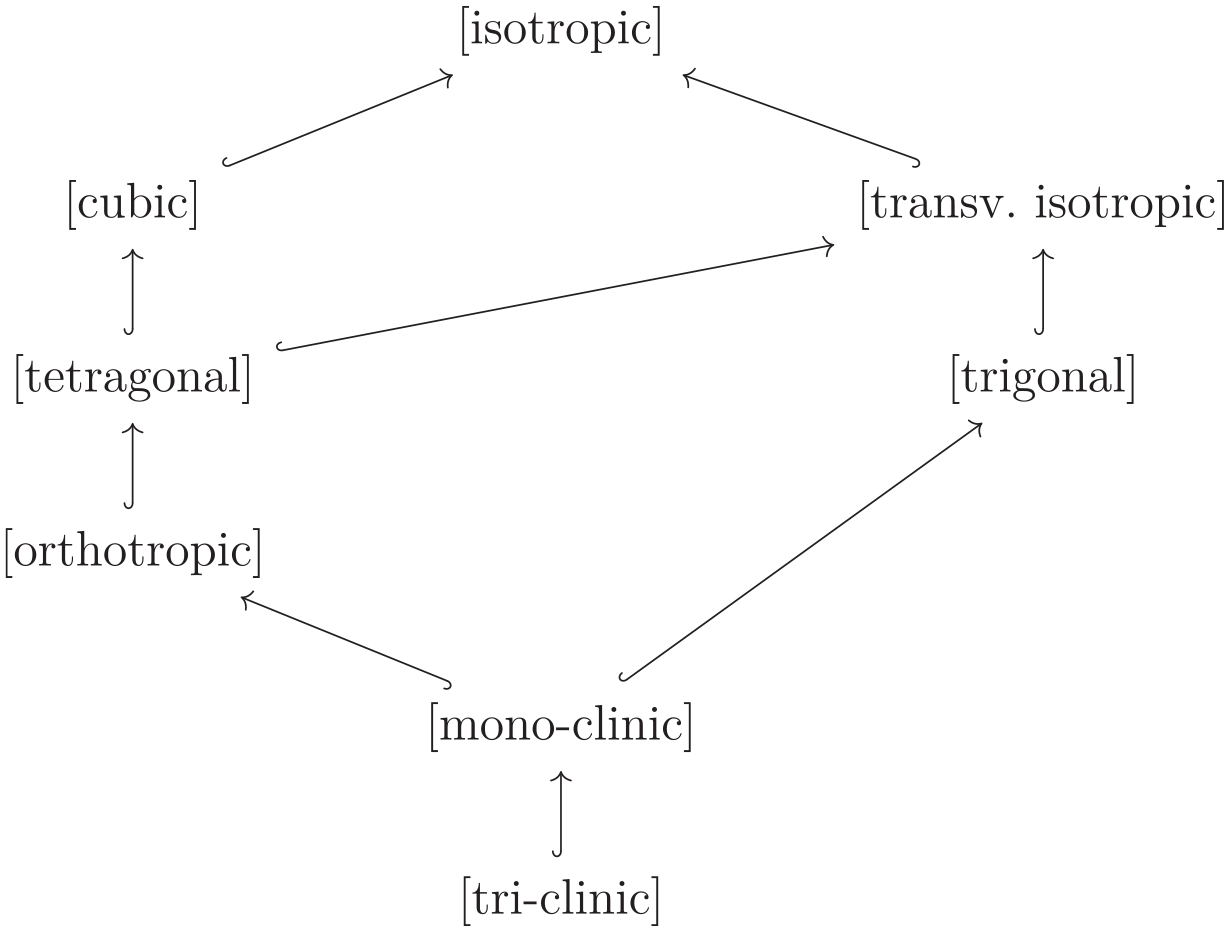
In 2D, there are four symmetry classes [15], to be shortly and informally described by pointing out a geometric figure with the same symmetry. The Hasse diagram—drawn horizontally in Figure 1—shows the relation of the lattice of elasticity symmetry or invariance groups as subgroups of the full orthogonal group, where the hooked arrow means a subgroup relation, e.g., the symmetry group of the orthotropic class is a subgroup of the symmetry group of the tetragonal class. The largest group is on the left, the isotropic class with the symmetries of a circle (i.e., the whole 2D rotation group), then the next smaller one is the tetragonal class with the symmetry of a square, then the orthotropic class with the symmetry of a general rectangle, and finally the tri-clinic class with the symmetry of a parallelogram.

Figure 1.

Hasse diagram of symmetry subgroups of fourth-order tensors in 2D.

4.1.1. Tri-clinic material in 2D

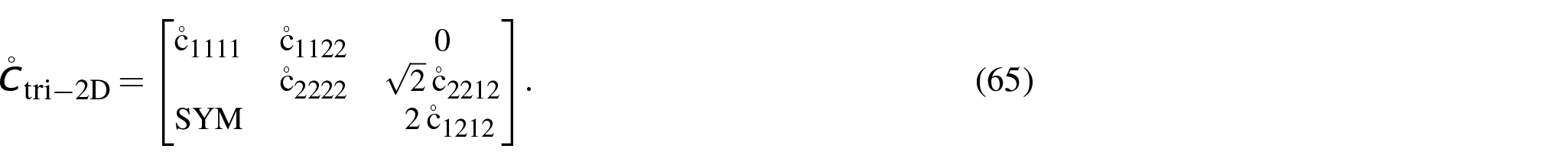
This section covers not only tri-clinic, but also mono-clinic materials, as there is no difference in 2D. As mentioned before, these materials have in 2D the symmetry of a parallelogram. The Kelvin matrix C cannot be simplified through a group reduction with a spatial rotation $\mathsf{Q}\in \mathrm{ST}(\mathcal{T})$ to a block-diagonal form beyond the general form equation (13), where one may note that there are $n=6=\dim \mathcal{E}=\dim \mathcal{S}$ free parameters. But, as in 2D one has $\dim \mathrm{ST}(\mathcal{T})=\dim \mathfrak{s}\mathfrak{t}(\mathcal{T})=1$ , one parameter $\mathit{q}=(\theta )\in \mathcal{Q}\equiv {\mathrm{ℝ}}^{m_Q}$ ( $m_Q=1$ ) may be used for a spatial rotation, see equations (117) and (120) in Appendix 2, to induce one zero in the upper right corner [35], this echos the first of the relations in equation (35):

$${\stackrel{°}{\mathsf{C}}}_{\mathrm{tri}-2D}=\left[\begin{array}{ccc}\hfill {\stackrel{°}{\mathrm{c}}}_{1111}\hfill & \hfill {\stackrel{°}{\mathrm{c}}}_{1122}\hfill & \hfill 0\hfill \\ \hfill & \hfill {\stackrel{°}{\mathrm{c}}}_{2222}\hfill & \hfill \sqrt{2}{\stackrel{°}{\mathrm{c}}}_{2212}\hfill \\ \hfill \mathrm{SYM}\hfill & \hfill & \hfill 2{\stackrel{°}{\mathrm{c}}}_{1212}\hfill \end{array}\right].$$

(65)

The spatial rotations $\mathit{Q}\in \mathrm{SO}(\mathcal{V})$ resp. $\mathsf{Q}\in \mathrm{ST}(\mathcal{T})$ decide on whether the spatial orientation of the material axes changes or not. Hence, one wants to keep this possibility in the stochastic modelling process.

What is needed next is to use the spectral decomposition of $\stackrel{°}{\mathsf{C}}$ , the second of the relations in equation (35). The matrix in equation (65) has generally three distinct positive eigenvalues ${\lambda }_1,{\lambda }_2$ , and ${\lambda }_3$ . For the three distinct eigenvalues one thus needs $m_{\mathrm{\Lambda }}=3$ log-eigenvalue parameters ${\mathrm{ℝ}}^{m_{\mathrm{\Lambda }}}\ni \mathit{\mu }=({\mu }_1,{\mu }_2,{\mu }_3)\mapsto \mathsf{M}=\mathrm{diag}(\mathit{\mu })$ , such that $\mathsf{\Lambda }(\mathit{\mu })=\mathrm{diag}({\lambda }_1,{\lambda }_2,{\lambda }_3)=\exp \mathsf{M}$ .

The Kelvin matrix $\stackrel{°}{\mathsf{C}}$ in equation (65) can of course be diagonalised as in equation (18), but the corresponding matrix of eigenvectors $\mathsf{V}\in \mathrm{SO}(\mathcal{T})$ is not in $\mathrm{ST}(\mathcal{T})$ , i.e., not induced by a spatial rotation.

In Section 3.1, it was explained how to keep the spatial rotation described by $\mathcal{Q}\ni \mathit{q}\mapsto \mathit{Q}\mapsto \mathit{Q}$ —cf. ‘Rotations in $\mathrm{SO}(\mathcal{T})$ ’ in Appendix 2—from interfering with the ‘strain distributor’ part $\mathsf{V}\in \mathrm{SO}(\mathcal{T})$ by introducing the orthogonal split in the corresponding Lie algebra already mentioned in equation (42): $\mathfrak{s}\mathfrak{o}(\mathcal{T})=\mathfrak{s}\mathfrak{t}(\mathcal{T})\oplus \mathfrak{s}\mathfrak{t}{(\mathcal{T})}^{\perp }$ . As just mentioned, in 2D one has $\dim \mathfrak{s}\mathfrak{t}(\mathcal{T})=1=m_Q$ , and this is needed for the rotation angle parameter $\mathit{q}=(\theta )\in \mathcal{Q}$ to describe the spatial rotation. This means $m_V=n-m_Q-m_{\mathrm{\Lambda }}=6-1-3=2=\dim \mathfrak{s}\mathfrak{t}{(\mathcal{T})}^{\perp }$ angle-like parameters $\mathit{p}=(s_1,s_2)\in {\mathcal{Q}}^{\perp }\equiv {\mathrm{ℝ}}^{m_V}$ can now be used to describe the eigenvectors of the Kelvin matrix in equation (65), i.e., the columns of $\mathsf{V}\in \mathrm{SO}(\mathcal{T})$ in equation (18).

There are at least two ways of generating such a $\mathsf{V}\in \mathrm{SO}(\mathcal{T})$ : one is to use the equations (121) and (122) in ’Rotations in $\mathrm{SO}(\mathcal{T})$ ’ in Appendix 2, where the parameters $\mathit{p}\in {\mathcal{Q}}^{\perp }$ are directly used for a map ${\mathcal{Q}}^{\perp }\to \mathfrak{s}\mathfrak{t}{(\mathcal{T})}^{\perp }\to \mathrm{SO}(\mathcal{T})$ to generate a $\mathsf{V}(\mathit{p})=\mathsf{V}(s_1,s_2)\in \mathrm{SO}(\mathcal{T})$ . Another way is to use two 2D rotation matrices—cf. equation (105)—embedded in 3D depending on angles $\mathit{p}=(s_1,s_2)$ :

$${\mathsf{V}}_i(s_1):=\left[\begin{array}{ccc}\hfill 1\hfill & \hfill 0\hfill & \hfill 0\hfill \\ \hfill 0\hfill & \hfill \cos s_1\hfill & \hfill -\sin s_1\hfill \\ \hfill 0\hfill & \hfill \sin s_1\hfill & \hfill \cos s_1\hfill \end{array}\right];{\mathsf{V}}_{\mathrm{ii}}(s_2):=\left[\begin{array}{ccc}\hfill \cos s_2\hfill & \hfill -\sin s_2\hfill & \hfill 0\hfill \\ \hfill \sin s_2\hfill & \hfill \cos s_2\hfill & \hfill 0\hfill \\ \hfill 0\hfill & \hfill 0\hfill & \hfill 1\hfill \end{array}\right].$$

(66)

Here the explicit formulation of the skew matrices ${\mathsf{P}}_i,{\mathsf{P}}_{\mathrm{ii}}\in \mathfrak{s}\mathfrak{t}(\mathcal{T})$ and the explicit use of the exponential map in the mapping chain $\mathit{p}\mapsto \mathsf{P}\mapsto \mathsf{V}$ according to ’Rotations in $\mathrm{SO}(\mathcal{V})$ in 3D and 2D’ in Appendix 2 has been shortened by giving just the final result. Then with $\mathsf{V}(\mathit{p})=\mathsf{V}(s_1,s_2)={\mathsf{V}}_i(s_1){\mathsf{V}}_{\mathrm{ii}}(s_2)$ it is easily seen that (cf. equation (18))

$$\stackrel{°}{\mathsf{C}}(\mathit{\mu },\mathit{p})=\mathsf{V}(\mathit{p})\mathsf{\Lambda }(\mathit{\mu }){\mathsf{V}}^{\mathsf{T}}(\mathit{p})$$

(67)

has the form equation (65), which corresponds to the spectral decomposition as the second of the relations in equation (35). In both cases, the parameters $\mathit{p}=(s_1,s_2)$ are purely a description of the distribution of eigen-strains for the material specification. Note that the first column of the matrix ${\mathsf{v}}_1$ of $\mathsf{V}=\left[{\mathsf{v}}_1{\mathsf{v}}_2{\mathsf{v}}_3\right]$ is the eigenvector or eigen-strain for the eigenvalue ${\lambda }_1$ , ${\mathsf{v}}_2$ the eigenvector of ${\lambda }_2$ , and so on. If one wants to distinguish the bulk or volumetric response from the shear response, e.g., by assigning the largest of the eigenvalues to this response, then one may choose the eigenvector ${\mathsf{v}}_j$ which has the largest projection onto the volumetric strain n (equation (132) in ’Kelvin notation’ in Appendix (3)). By assigning the largest eigenvalue to that eigenvector—it was described previously how to generate random eigenvalues where one is always larger than the others—one can ascertain that the bulk or volumetric response is always stiffer than the shear response.

By construction, the form in equation (67) is invariant under rotations in the symmetry group ${\mathfrak{S}}_{\mathsf{C}}=\mathsf{Trep}({\mathfrak{S}}_{\mathbf{c}})=\left[\mathrm{tri-clinic}\right]$ . Finally, the elasticity matrix for a tri-clinic material in 2D with the proper spatial orientation $\mathit{q}=(\theta )$ may be generated from equation (67) in a two-step rotation procedure via

$$\begin{array}{ccc}\hfill {\mathsf{C}}_{\mathrm{tri}-2D}(\mathit{q},\mathit{\mu },\mathit{p})& ={\mathsf{Q}}^{\mathsf{T}}(\mathit{q})\stackrel{°}{\mathsf{C}}(\mathit{\mu },\mathit{p})\mathsf{Q}(\mathit{q}),\mathrm{or}\mathrm{even}\mathrm{in}\mathrm{more}\mathrm{detail}\hfill & \hfill \\ \hfill & ={\mathsf{Q}}_0^{\mathsf{T}}{\mathsf{Q}}_1^{\mathsf{T}}(\mathit{q}){\mathsf{V}}_1(\mathit{p}){\mathsf{V}}_0{\mathsf{\Lambda }}_0{\mathsf{\Lambda }}_1(\mathit{\mu }){\mathsf{V}}_0^{\mathsf{T}}{\mathsf{V}}_1^{\mathsf{T}}(\mathit{p}){\mathsf{Q}}_1(\mathit{q}){\mathsf{Q}}_0.\hfill & \hfill & \hfill \end{array}$$

(68)

The last equation in equation (68)—the third of the relations in equation (35)—is the concrete version of equation (53) in Section 3.4. One may recall that $\hat{\mathsf{C}}={\mathsf{Q}}_0^{\mathsf{T}}{\mathsf{V}}_0{\mathsf{\Lambda }}_0{\mathsf{V}}_0^{\mathsf{T}}{\mathsf{Q}}_0$ is the constant reference matrix — e.g. the scaling-rotation mean—which may be actually invariant under a larger symmetry group ${\mathfrak{S}}_{\mathsf{C},m}=\mathsf{Trep}({\mathfrak{S}}_{\mathbf{c},m})\supset {\mathfrak{S}}_{\mathsf{C}}$ , i.e., further to the left in Figure 1. In case one of the eigenvectors is a pure shear, i.e., proportional to y in equation (133) in ’Kelvin notation’ in Appendix 3, then the material is in fact orthotropic, to be described next.

4.1.2. Orthotropic material in 2D

As already indicated, such materials have the symmetry of a general rectangle in 2D. By the group reduction process, i.e., a spatial rotation $\mathsf{Q}\in \mathrm{ST}(\mathcal{T})$ given by one parameter $\mathit{q}=(\theta )\in \mathcal{Q}\equiv {\mathrm{ℝ}}^{m_Q}$ ( $m_Q=1$ ), see equations (117) and (120) in Appendix 2, the Kelvin matrix for these materials may be brought into the following block-diagonal form [35], with four free parameters:

$${\stackrel{°}{\mathsf{C}}}_{\mathrm{ortho}-2D}=\left[\begin{array}{ccc}\hfill {\stackrel{°}{\mathrm{c}}}_{1111}\hfill & \hfill {\stackrel{°}{\mathrm{c}}}_{1122}\hfill & \hfill 0\hfill \\ \hfill & \hfill {\stackrel{°}{\mathrm{c}}}_{2222}\hfill & \hfill 0\hfill \\ \hfill \mathrm{SYM}\hfill & \hfill & \hfill 2{\stackrel{°}{\mathrm{c}}}_{1212}\hfill \end{array}\right],$$

(69)

which has one obvious eigen-stiffness or Kelvin shear modulus ${\lambda }_3=2{\stackrel{°}{\mathrm{c}}}_{1212}$ with associated eigenvector or eigen-strain distributor

$${\mathsf{v}}_3={[0,0,1]}^{\mathsf{T}},$$

(70)

a simple shear. The other two come from the diagonalisation of the upper $2\times 2$ upper left sub-matrix of equation (69), and have the general form of a rotation of $\mathsf{n},\mathsf{y}$ in equations (132) and (133) about the fixed vector ${\mathsf{v}}_3$ in equation (70) in the strain-representer space $\mathcal{T}$ :

$${\mathsf{v}}_1(s)={[\cos s,\sin s,0]}^{\mathsf{T}}\mathrm{and}{\mathsf{v}}_2(s)={[-\sin s,\cos s,0]}^{\mathsf{T}},$$

(71)

associated with the other two Kelvin moduli ${\lambda }_1,{\lambda }_2$ . Observe that the single parameter $\mathit{p}=(s)\in {\mathcal{Q}}^{\perp }\equiv {\mathrm{ℝ}}^{m_V}$ ( $m_V=1$ ) is not an angle in a spatial sense, but is one in the two-dimensional strain representer subspace formed by the first two components, characterising the material, or more precisely, the Kelvin eigen-strains. Here, as just before, the mapping chain $\mathit{p}\mapsto \mathsf{P}\mapsto \mathsf{V}$ according to ’Rotations in $\mathrm{SO}(\mathcal{V})$ in 3D and 2D’ in Appendix 2 has been shortened to display just the final result $\mathsf{V}(\mathit{p})$ .

The previous remarks made for tri-clinic material regarding the possible choice of the largest Kelvin module to be associated with the volumetric response apply here as well. Again, for the three generally distinct eigenvalues one needs $m_{\mathrm{\Lambda }}=3$ log-eigenvalue parameters ${\mathrm{ℝ}}^{m_{\mathrm{\Lambda }}}\ni \mathit{\mu }=({\mu }_1,{\mu }_2,{\mu }_3)\mapsto \mathsf{M}=\mathrm{diag}(\mathit{\mu })$ , such that $\mathsf{\Lambda }(\mathit{\mu })=\mathrm{diag}({\lambda }_1,{\lambda }_2,{\lambda }_3)=\exp \mathsf{M}$ . In addition, one has with equations (70) and (71) $\mathsf{V}(\mathit{p})=\mathsf{V}(s)=[{\mathsf{v}}_1(s){\mathsf{v}}_2(s){\mathsf{v}}_3]$ , and with that formally the same kind of spectral representation as in equation (67) for ${\stackrel{°}{\mathsf{C}}}_{\mathrm{ortho}-2D}(\mathit{\mu },\mathit{p})$ . The Kelvin elasticity matrix ${\mathsf{C}}_{\mathrm{ortho}-2D}(\mathit{q},\mathit{\mu },\mathit{p})$ for an orthotropic material in 2D with the proper spatial orientation $\mathit{q}=(\theta )$ may then again be generated as in equation (53) in Section 3.4, or in equation (68) in a two-step rotation procedure, see also the remarks there. The total number of parameters $(\mathit{q},\mathit{\mu },\mathit{p})$ is $n=m_Q+m_{\mathrm{\Lambda }}+m_V=1+3+1=5$ . In case $s=\pi ∕4$ in equation (71), i.e., in case the first two eigenvectors are ${\mathsf{v}}_1=\mathsf{n}$ and ${\mathsf{v}}_2=\mathsf{y}$ , the material is actually tetragonal.

4.1.3. Tetragonal material in 2D

As already indicated, such materials have the symmetry of a square in 2D. Again, by the group reduction process and a spatial rotation given by one parameter $\mathit{q}=(\theta )\in \mathcal{Q}\equiv {\mathrm{ℝ}}^{m_Q}$ ( $m_Q=1$ ), the Kelvin matrix for these materials may be brought into the following block-diagonal form [35], with three free parameters:

$${\stackrel{°}{\mathsf{C}}}_{\mathrm{tetra}-2D}=\left[\begin{array}{ccc}\hfill {\stackrel{°}{\mathrm{c}}}_{1111}\hfill & \hfill {\stackrel{°}{\mathrm{c}}}_{1122}\hfill & \hfill 0\hfill \\ \hfill & \hfill {\stackrel{°}{\mathrm{c}}}_{1111}\hfill & \hfill 0\hfill \\ \hfill \mathrm{SYM}\hfill & \hfill & \hfill 2{\stackrel{°}{\mathrm{c}}}_{1212}\hfill \end{array}\right],$$

(72)

completely determining the spectral decomposition, with, as before in the 2D orthotropic case with the obvious Kelvin shear modulus ${\lambda }_3=2{\stackrel{°}{\mathrm{c}}}_{1212}$ and eigenvector ${\mathsf{v}}_3$ as in equation (70), and the two additional generally distinct Kelvin moduli ( $m_{\mathrm{\Lambda }}=3$ ): ${\lambda }_1={\stackrel{°}{\mathrm{c}}}_{1111}+{\stackrel{°}{\mathrm{c}}}_{1122}$ and ${\lambda }_2=\stackrel{°}{{\mathrm{c}}_{1111}}-{\stackrel{°}{\mathrm{c}}}_{1122}$ , i.e., ${\lambda }_1={\lambda }_2+2{\stackrel{°}{\mathrm{c}}}_{1122}$ .

The associated eigenvectors are fixed ( $m_V=0$ ), corresponding to $s=\pi ∕4$ in equation (71): ${\mathsf{v}}_1=\mathsf{n}$ and ${\mathsf{v}}_2=\mathsf{y}$ , cf. equations (132) and (133), hence $\mathsf{V}=\left[{\mathsf{v}}_1{\mathsf{v}}_2{\mathsf{v}}_3\right]$ is a fixed matrix. As is easily observed, ${\lambda }_1$ is a volumetric Kelvin modulus, whereas ${\lambda }_2$ is a shear Kelvin modulus; and the previous remarks made for tri-clinic material regarding the possible choice of the largest Kelvin module to be associated with the volumetric response apply here as well.

Here again, for the three generally distinct eigenvalues one needs $m_{\mathrm{\Lambda }}=3$ log-eigenvalue parameters $\mathit{\mu }=({\mu }_1,{\mu }_2,{\mu }_3)$ . With the above fixed V one obtains formally the same kind of spectral representation as in equation (67) for ${\stackrel{°}{\mathsf{C}}}_{\mathrm{tetra}-2D}(\mathit{\mu })$ in equation (72). The tetragonal 2D Kelvin elasticity matrix ${\mathsf{C}}_{\mathrm{tetra}-2D}(\mathit{q},\mathit{\mu })$ with the proper spatial orientation $\mathit{q}=(\theta )$ may then again be generated as in equation (53) in Section 3.4, or in equation (68) in a two-step rotation procedure. The total number of parameters $(\mathit{q},\mathit{\mu })$ is $n=m_Q+m_{\mathrm{\Lambda }}+m_V=1+3+0=4$ . In case the two shear Kelvin moduli coincide, i.e., ${\lambda }_2={\lambda }_3$ , the material is actually isotropic.

4.1.4. Isotropic material in 2D

As already mentioned, such a material has the symmetry group of a circle in 2D. This means that no spatial rotation is needed ( $m_Q=0$ ) to bring the Kelvin matrix to the block-diagonal form equation (72) with ${\lambda }_3=2{\stackrel{°}{\mathrm{c}}}_{1212}={\stackrel{°}{\mathrm{c}}}_{1111}-{\stackrel{°}{\mathrm{c}}}_{1122}={\lambda }_2$ , the Kelvin matrix has this form in any spatial orientation. Thus there are only two ( $n=m_Q+m_{\mathrm{\Lambda }}+m_V=0+2+0=2$ ) free parameters for the two log-eigenvalues ${\mu }_1,{\mu }_2={\mu }_3$ . The spectral decomposition as in equation (67) with the matrix V as in the tetragonal case is the final product ${\stackrel{°}{\mathsf{C}}}_{\mathrm{iso}-2D}$ , no spatial rotations as in equation (53) in Section 3.4, or in equation (68) are necessary, as the Kelvin matrix ${\stackrel{°}{\mathsf{C}}}_{\mathrm{iso}-2D}$ is invariant under such rotations.

4.2. Elasticity classes in 3D

In 3D, there are eight elasticity classes [8–11,14,35,49–51]. The Hasse diagram for 3D in Figure 2 shows the relation of the lattice of elasticity symmetry or invariance groups as subgroups of the full orthogonal group in 3D. They will be again described informally by pointing out geometric bodies with the same symmetry. On top is the isotropic class with the symmetries of a sphere, i.e., the whole orthogonal group, with the sub-classes—descending in the Hasse diagram in Figure 2 along the left branch—the cubic class with the symmetries of a cube, the tetragonal class with the symmetries of a square prism (a right prism with a square base), the orthotropic class with the symmetries of a right prism (a right prism with a general rectangle as base), the mono-clinic class with the symmetries of a right prism with a parallelogram as base, and the tri-clinic class with the symmetries of a parallelepiped (an oblique prism with a parallelogram as base). On the right branch of the Hasse diagram for 3D in Figure 2 are the transversely isotropic class with the symmetries of a circular cylinder and the trigonal class with the symmetries of a triangular prism (a right prism with a equilateral triangle as base).

Figure 2.

Hasse diagram of symmetry subgroups of fourth-order tensors in 3D.

4.2.1. Tri-clinic material in 3D

As mentioned before, these materials have in 3D the symmetry of a parallelepiped. As in the 2D case for tri-clinic materials, the Kelvin matrix C cannot be simplified through a group reduction with a spatial rotation $\mathsf{Q}=\mathsf{Trep}(\mathit{Q})\in \mathrm{ST}(\mathcal{T})$ to a block-diagonal form beyond the general form equation (12), and there are $n=21$ free parameters. But, as in 3D one has $\dim \mathrm{ST}(\mathcal{T})=\dim \mathfrak{s}\mathfrak{t}(\mathcal{T})=3$ , three parameters $\mathit{q}=(q_1,q_2,q_3)\in \mathcal{Q}\equiv {\mathrm{ℝ}}^{m_Q}\subset {\mathrm{ℝ}}^{15}$ ( $m_Q=3$ ) may be used for a spatial rotation, the direction of the vector q actually being the rotation axis of $\mathit{Q}(\mathit{q})\in \mathrm{SO}(3)$ , see equations (108) and (115) in Appendix 2, to induce three zeros in the right of the top row [35], this echos the first of the relations in equation (35):

$${\stackrel{°}{\mathsf{C}}}_{\mathrm{tri-3D}}=\left[\begin{array}{cccccc}\hfill {\stackrel{°}{\mathrm{c}}}_{1111}\hfill & \hfill {\stackrel{°}{\mathrm{c}}}_{1122}\hfill & \hfill {\stackrel{°}{\mathrm{c}}}_{1133}\hfill & \hfill 0\hfill & \hfill 0\hfill & \hfill 0\hfill \\ \hfill & \hfill {\stackrel{°}{\mathrm{c}}}_{2222}\hfill & \hfill {\stackrel{°}{\mathrm{c}}}_{2233}\hfill & \hfill \sqrt{2}{\stackrel{°}{\mathrm{c}}}_{2223}\hfill & \hfill \sqrt{2}{\stackrel{°}{\mathrm{c}}}_{2213}\hfill & \hfill \sqrt{2}{\stackrel{°}{\mathrm{c}}}_{2212}\hfill \\ \hfill & \hfill & \hfill {\stackrel{°}{\mathrm{c}}}_{3333}\hfill & \hfill \sqrt{2}{\stackrel{°}{\mathrm{c}}}_{3323}\hfill & \hfill \sqrt{2}{\stackrel{°}{\mathrm{c}}}_{3313}\hfill & \hfill \sqrt{2}{\stackrel{°}{\mathrm{c}}}_{3312}\hfill \\ \hfill & \hfill & \hfill & \hfill 2{\stackrel{°}{\mathrm{c}}}_{2323}\hfill & \hfill 2{\stackrel{°}{\mathrm{c}}}_{2313}\hfill & \hfill 2{\stackrel{°}{\mathrm{c}}}_{2312}\hfill \\ \hfill & \hfill \mathrm{SYM}\hfill & \hfill & \hfill & \hfill 2{\stackrel{°}{\mathrm{c}}}_{1313}\hfill & \hfill 2{\stackrel{°}{\mathrm{c}}}_{1312}\hfill \\ \hfill & \hfill & \hfill & \hfill & \hfill & \hfill 2{\stackrel{°}{\mathrm{c}}}_{1212}\hfill \end{array}\right].$$

(73)

As before in 2D, the spatial rotations $\mathit{Q}\in \mathrm{SO}(\mathcal{V})$ resp. $\mathsf{Q}\in \mathrm{ST}(\mathcal{T})$ decide on whether the spatial orientation of the material axes changes or not, and thus one wants to keep this possibility in the stochastic modelling process.

The matrix in equation (73) has generally six distinct positive eigenvalues ${\lambda }_1,\dots ,{\lambda }_6$ , for which one needs $m_{\mathrm{\Lambda }}=6$ log-eigenvalue parameters to generate the diagonal eigenvalue matrix: ${\mathrm{ℝ}}^{m_{\mathrm{\Lambda }}}\ni \mathit{\mu }=({\mu }_1,\dots ,{\mu }_6)\mapsto \mathsf{M}=\mathrm{diag}(\mathit{\mu })\mapsto \mathsf{\Lambda }(\mathit{\mu })=\mathrm{diag}({\lambda }_j)=\exp \mathsf{M}$ .

Next one wants to use the spectral decomposition of ${\stackrel{°}{\mathsf{C}}}_{\mathrm{tri-3D}}$ , the second of the relations in equation (35). As a $\mathsf{Q}\in \mathrm{ST}(\mathcal{T})$ was used to generate the special form equation (73), this matrix can be diagonalised as in equation (18), but the corresponding matrix of eigenvectors $\mathsf{V}\in \mathrm{SO}(\mathcal{T})$ is not induced by a spatial rotation, and thus generated by a $\mathsf{P}\in \mathfrak{s}\mathfrak{t}{(\mathcal{T})}^{\perp }$ . See Section 3.1 on how to keep the spatial rotation Q from interfering with the ‘strain distributor’ part $\mathsf{V}\in \mathrm{SO}(\mathcal{T})$ by introducing the orthogonal split in the corresponding Lie algebra already mentioned in equation (42): $\mathfrak{s}\mathfrak{o}(\mathcal{T})=\mathfrak{s}\mathfrak{t}(\mathcal{T})\oplus \mathfrak{s}\mathfrak{t}{(\mathcal{T})}^{\perp }$ . As $\dim \mathfrak{s}\mathfrak{t}{(\mathcal{T})}^{\perp }=m_V=n-m_Q-m_{\mathrm{\Lambda }}=12$ , all that is needed now is a basis of the space ${\mathcal{Q}}^{\perp }$ , given in equation (116) in ’Rotations in $\mathrm{SO}(\mathcal{T})$ ’ in Appendix 2. With that basis $\{{\mathit{k}}_1,\dots ,{\mathit{k}}_{12}\}$ and 12 parameters $(s_1,\dots ,s_{12})$ one may form the vector $\mathit{p}={\mathrm{\sum }}_{j=1}^{12}{s}_j{\mathit{k}}_j\in {\mathcal{Q}}^{\perp }$ , and then map this on to $\mathit{p}\mapsto \mathsf{P}(\mathit{p})\in \mathfrak{s}\mathfrak{t}{(\mathcal{T})}^{\perp }$ according to equation (108). This is finally mapped to $\mathsf{V}(\mathit{p})=\exp \mathsf{P}(\mathit{p})$ , to obtain ${\stackrel{°}{\mathsf{C}}}_{\mathrm{tri-3D}}(\mathit{\mu },\mathit{p})$ as in equation (67), which corresponds to the spectral decomposition as the second of the relations in equation (35).

The columns of the matrix $\mathsf{V}=[{\mathsf{v}}_1,\dots ,{\mathsf{v}}_6]$ are the eigenvectors corresponding to the eigenvalues ${\lambda }_1,\dots ,{\lambda }_6$ . As before, in case one wants to distinguish the bulk or volumetric response from the shear response, e.g., by assigning the largest of the eigenvalues to this response, then one may choose the eigenvector ${\mathsf{v}}_j$ which has the largest projection onto the volumetric strain n given in equation (126) in ’Kelvin notation’ in Appendix 3, and assign the largest eigenvalue to that eigenvector.

Finally, as before, the two-step rotation procedure with a spatial rotation $\mathsf{Q}(\mathit{q})$ given by $\mathit{q}\in \mathcal{Q}$ may be used as in equation (68) to rotate the Kelvin matrix to the desired coordinate system. As pointed out before, the last equation in equation (68) giving ${\mathsf{C}}_{\mathrm{tri-3D}}(\mathit{q},\mathit{\mu },\mathit{p})$ here—the third relation in equation (35)—is the concrete version of equation (53) in Section 3.4, cf. the remarks for tri-clinic materials in 2D in Section 4.1. In case two of the eigenvectors are pure shears, i.e., proportional to y in equation (127) and z in equation (128) in ’Kelvin notation’ in Appendix 3, or some linear combination thereof, then the material is in fact mono-clinic, to be described next.

4.2.2. Mono-clinic material in 3D

As indicated previously, these materials have in 3D the symmetry of a right prism with a parallelogram as base. In this case [35], the Kelvin matrix C can be simplified through a group reduction with a spatial rotation $\mathsf{Q}\in \mathrm{ST}(\mathcal{T})$ to a block-diagonal form with three diagonal blocks equation (74), and in this form there are $12$ free parameters. An additional $m_Q=\dim \mathrm{ST}(\mathcal{T})=\dim \mathfrak{s}\mathfrak{t}(\mathcal{T})=3$ parameters $\mathit{q}=(q_1,q_2,q_3)\in \mathcal{Q}\equiv {\mathrm{ℝ}}^{m_Q}$ are used for the spatial rotation $\mathsf{Q}(\mathit{q})$ just referenced for the group reduction process, giving the total number of parameters for mono-clinic material as $n=15$ ; see equations (108) and (115) in Appendix 2, this is the first relation in equation (35):

$${\stackrel{°}{\mathsf{C}}}_{\mathrm{mono-3D}}=\left[\begin{array}{cccccc}\hfill {\stackrel{°}{\mathrm{c}}}_{1111}\hfill & \hfill {\stackrel{°}{\mathrm{c}}}_{1122}\hfill & \hfill {\stackrel{°}{\mathrm{c}}}_{1133}\hfill & \hfill \sqrt{2}{\stackrel{°}{\mathrm{c}}}_{1123}\hfill & \hfill 0\hfill & \hfill 0\hfill \\ \hfill & \hfill {\stackrel{°}{\mathrm{c}}}_{2222}\hfill & \hfill {\stackrel{°}{\mathrm{c}}}_{2233}\hfill & \hfill \sqrt{2}{\stackrel{°}{\mathrm{c}}}_{2223}\hfill & \hfill 0\hfill & \hfill 0\hfill \\ \hfill & \hfill & \hfill {\stackrel{°}{\mathrm{c}}}_{3333}\hfill & \hfill \sqrt{2}{\stackrel{°}{\mathrm{c}}}_{3323}\hfill & \hfill 0\hfill & \hfill 0\hfill \\ \hfill & \hfill & \hfill & \hfill 2{\stackrel{°}{\mathrm{c}}}_{2323}\hfill & \hfill 0\hfill & \hfill 0\hfill \\ \hfill & \hfill \mathrm{SYM}\hfill & \hfill & \hfill & \hfill 2{\stackrel{°}{\mathrm{c}}}_{1313}\hfill & \hfill 0\hfill \\ \hfill & \hfill & \hfill & \hfill & \hfill & \hfill 2{\stackrel{°}{\mathrm{c}}}_{1212}\hfill \end{array}\right].$$

(74)

The matrix in equation (74) has generally six distinct positive eigenvalues ${\lambda }_1,\dots ,{\lambda }_6$ , for which one needs, as before, $m_{\mathrm{\Lambda }}=6$ log-eigenvalue parameters to generate the diagonal eigenvalue matrix: $\mathit{\mu }=({\mu }_1,\dots ,{\mu }_6)\mapsto \mathsf{M}=\mathrm{diag}(\mathit{\mu })\mapsto \mathsf{\Lambda }(\mathit{\mu })=\mathrm{diag}({\lambda }_j)=\exp \mathsf{M}$ . Two eigenvalues are immediately recognisable from equation (74), namely the Kelvin moduli ${\lambda }_5=2{\stackrel{°}{\mathrm{c}}}_{1313}$ and ${\lambda }_6=2{\stackrel{°}{\mathrm{c}}}_{1212}$ with corresponding eigenvectors ${\mathsf{v}}_5={[0,0,0,0,1,0]}^{\mathsf{T}}$ and ${\mathsf{v}}_5={[0,0,0,0,0,1]}^{\mathsf{T}}$ .

The other four eigenvectors in $\mathsf{V}={[{\mathsf{v}}_1,\dots ,{\mathsf{v}}_4,{\mathsf{v}}_5,{\mathsf{v}}_6]}^{\mathsf{T}}$ come from the diagonalisation of the upper left $4\times 4$ block $\check{\mathsf{C}}$ in equation (74). This has a spectral decomposition $\check{\mathsf{C}}=\check{\mathsf{V}}\check{\mathsf{\Lambda }}{\check{\mathsf{V}}}^{\mathsf{T}}$ with $\check{\mathsf{V}}\in \mathrm{SO}(4)$ . As $\dim \mathrm{SO}(4)=\dim \mathfrak{s}\mathfrak{o}(4)=6$ , one needs $m_V=6=n-m_{\mathrm{\Lambda }}-m_Q$ additional parameters $\mathit{p}={[s_1,\dots ,s_6]}^{\mathsf{T}}\in {\mathcal{Q}}^{\perp }\equiv {\mathrm{ℝ}}^{m_V}$ to model this. Taking the four-dimensional version of equation (108) in ’Rotations in $\mathrm{SO}(\mathcal{T})$ ’ in Appendix 2, this is mapped to $\check{\mathsf{P}}(\mathit{p})\in \mathfrak{s}\mathfrak{o}(4)$ , and this on to $\check{\mathsf{V}}(\mathit{p})=\exp \check{\mathsf{P}}(\mathit{p})\in \mathrm{SO}(4)$ , yielding the eigen-strains of the eigenvalues resp. Kelvin moduli of $\check{\mathsf{C}}$ . Each column ${\check{\mathsf{v}}}_j\in {\mathrm{ℝ}}^4,j=1,\dots ,4$ in $\check{\mathsf{V}}=[{\check{\mathsf{v}}}_1,{\check{\mathsf{v}}}_2,{\check{\mathsf{v}}}_3,{\check{\mathsf{v}}}_4]$ is then extended into ${\mathrm{ℝ}}^6$ by padding with two zeros: ${\mathsf{v}}_j(\mathit{p})={[{\check{\mathsf{v}}}_j^{\mathsf{T}}(\mathit{p}),0,0]}^{\mathsf{T}}\in {\mathrm{ℝ}}^6,j=1,\dots ,4$ to complete $\mathsf{V}(\mathit{p})$ .

From this eigen-strain matrix $\mathsf{V}(\mathit{p})$ and the diagonal $\mathsf{\Lambda }(\mathit{\mu })$ one then obtains a random mono-clinic Kelvin matrix of the form equation (74): ${\stackrel{°}{\mathsf{C}}}_{\mathrm{mono-3D}}(\mathit{\mu },\mathit{p})=\mathsf{V}(\mathit{p})\mathsf{\Lambda }(\mathit{\mu }){\mathsf{V}}^{\mathsf{T}}(\mathit{p})$ , as in equation (67), corresponding to the spectral decomposition as the second of the relations in equation (35). The by now familiar two-step rotation procedure with a spatial rotation $\mathsf{Q}(\mathit{q})$ given by $\mathit{q}\in \mathcal{Q}$ may be used as in equation (68) to rotate the Kelvin matrix to the desired coordinate system, and again the last equation in equation (68) yielding ${\mathsf{C}}_{\mathrm{mono-3D}}(\mathit{q},\mathit{\mu },\mathit{p})$ —the third relation in equation (35)—is the concrete version of equation (53) in Section 3.4. In case ${\mathsf{v}}_4={[0,0,0,1,0,0]}^{\mathsf{T}}$ , the material is in fact orthotropic.

4.2.3. Orthotropic material in 3D

It was already mentioned that these materials have in 3D the symmetry of a right prism—a prism with a general rectangle as base. As in all the previous cases, the group reduction process with a rotation $\mathsf{Q}(\mathit{q})=\mathsf{Trep}(\mathit{Q}(\mathit{q}))\in \mathrm{ST}(\mathcal{T})$ leads to a block-diagonal form equation (75) with three rotation axis parameters $\mathit{q}=(q_1,q_2,q_3)\in \mathcal{Q}\equiv {\mathrm{ℝ}}^{m_Q}$ ( $m_Q=3$ ), see equations (108) and (115) in Appendix 2. The resulting Kelvin matrix of the form [35]:

$${\stackrel{°}{\mathsf{C}}}_{\mathrm{ortho-3D}}=\left[\begin{array}{cccccc}\hfill {\stackrel{°}{\mathrm{c}}}_{1111}\hfill & \hfill {\stackrel{°}{\mathrm{c}}}_{1122}\hfill & \hfill {\stackrel{°}{\mathrm{c}}}_{1133}\hfill & \hfill 0\hfill & \hfill 0\hfill & \hfill 0\hfill \\ \hfill & \hfill {\stackrel{°}{\mathrm{c}}}_{2222}\hfill & \hfill {\stackrel{°}{\mathrm{c}}}_{2233}\hfill & \hfill 0\hfill & \hfill 0\hfill & \hfill 0\hfill \\ \hfill & \hfill & \hfill {\stackrel{°}{\mathrm{c}}}_{3333}\hfill & \hfill 0\hfill & \hfill 0\hfill & \hfill 0\hfill \\ \hfill & \hfill & \hfill & \hfill 2{\stackrel{°}{\mathrm{c}}}_{2323}\hfill & \hfill 0\hfill & \hfill 0\hfill \\ \hfill & \hfill \mathrm{SYM}\hfill & \hfill & \hfill & \hfill 2{\stackrel{°}{\mathrm{c}}}_{1313}\hfill & \hfill 0\hfill \\ \hfill & \hfill & \hfill & \hfill & \hfill & \hfill 2{\stackrel{°}{\mathrm{c}}}_{1212}\hfill \end{array}\right]$$

(75)

has $m_{\mathrm{\Lambda }}+m_V=9$ free parameters, so that together with the rotation axis q with $m_Q=3$ parameters, in total there are $n=m_Q+m_{\mathrm{\Lambda }}+m_V=12$ parameters.

The matrix in equation (75) has generally six distinct positive eigenvalues ${\lambda }_1,\dots ,{\lambda }_6$ , for which one needs, as before, $m_{\mathrm{\Lambda }}=6$ log-eigenvalue parameters to generate the diagonal eigenvalue matrix $\mathit{\mu }=({\mu }_1,\dots ,{\mu }_6)\mapsto \mathsf{M}=\mathrm{diag}(\mathit{\mu })\mapsto \mathsf{\Lambda }(\mathit{\mu })=\mathrm{diag}({\lambda }_j)=\exp \mathsf{M}$ . Three eigenvalues are obvious from equation (75), namely the Kelvin moduli ${\lambda }_4=2{\stackrel{°}{\mathrm{c}}}_{2323}$ , ${\lambda }_5=2{\stackrel{°}{\mathrm{c}}}_{1313}$ , and ${\lambda }_6=2{\stackrel{°}{\mathrm{c}}}_{1212}$ with corresponding eigenvectors ${\mathsf{v}}_4={[0,0,0,1,0,0]}^{\mathsf{T}}$ , ${\mathsf{v}}_5={[0,0,0,0,1,0]}^{\mathsf{T}}$ , and ${\mathsf{v}}_6={[0,0,0,0,0,1]}^{\mathsf{T}}$ .

The other three eigenvectors come from the diagonalisation of the upper left $3\times 3$ block $\check{\mathsf{C}}$ in equation (75). Its spectral decomposition is $\check{\mathsf{C}}=\check{\mathsf{V}}\check{\mathsf{\Lambda }}{\check{\mathsf{V}}}^{\mathsf{T}}$ with $\check{\mathsf{V}}\in \mathrm{SO}(3)$ . Therefore, $m_V=3=n-m_{\mathrm{\Lambda }}-m_Q$ additional parameters $\mathit{p}={[s_1,s_2,s_3]}^{\mathsf{T}}\in {\mathcal{Q}}^{\perp }\equiv {\mathrm{ℝ}}^{m_V}$ to model this. As $m_V=3$ , one may actually use Rodrigues original formula equations (102–104) in ’Rotations in $\mathrm{SO}(\mathcal{V})$ in 3D and 2D’ in Appendix 2, such that p is the rotation vector, but now in the strain representer space $\mathcal{T}$ , and not in physical space $\mathcal{V}.$ This produces a rotation matrix $\check{\mathsf{V}}(\mathit{p})=\exp \check{\mathsf{P}}(\mathit{p})\in \mathrm{SO}(3)$ , yielding the eigen-strains of the eigenvalues resp. Kelvin moduli of $\check{\mathsf{C}}$ . Each column ${\check{\mathsf{v}}}_j\in {\mathrm{ℝ}}^3$ in $\check{\mathsf{V}}=[{\check{\mathsf{v}}}_1,{\check{\mathsf{v}}}_2,{\check{\mathsf{v}}}_3]$ is then extended into ${\mathrm{ℝ}}^6$ by padding with three zeros: ${\mathsf{v}}_j(\mathit{p})={[{\check{\mathsf{v}}}_j^{\mathsf{T}}(\mathit{p}),0,0,0]}^{\mathsf{T}}\in {\mathrm{ℝ}}^6,j=1,\dots ,3$ to complete $\mathsf{V}(\mathit{p})$ . The familiar two-step rotation procedure with a spatial rotation $\mathsf{Q}(\mathit{q})$ given by $\mathit{q}\in \mathcal{Q}$ may be used as in equation (68) to rotate the Kelvin matrix to the desired coordinate system.

4.2.4. Trigonal material in 3D

It was already mentioned that these materials have in 3D the symmetry of a triangular prism. As in all the previous cases, the Kelvin matrix can be simplified in the group reduction process with a rotation $\mathsf{Q}(\mathit{q})=\mathsf{Trep}(\mathit{Q}(\mathit{q}))\in \mathrm{ST}(\mathcal{T})$ with three rotation axis parameters $\mathit{q}=(q_1,q_2,q_3)\in \mathcal{Q}\equiv {\mathrm{ℝ}}^{m_Q}$ ( $m_Q=3$ ) — a so-called natural coordinate system with the spatial three-axis equal to the three-fold rotation axis—into a form [35] with $n-m_Q=6$ free parameters (i.e., the total number of parameters is $n=9$ ):

$${\stackrel{°}{\mathsf{C}}}_{\mathrm{trigon-3D}}=\left[\begin{array}{cccccc}\hfill {\stackrel{°}{\mathrm{c}}}_{1111}\hfill & \hfill {\stackrel{°}{\mathrm{c}}}_{1122}\hfill & \hfill {\stackrel{°}{\mathrm{c}}}_{1133}\hfill & \hfill \sqrt{2}{\stackrel{°}{\mathrm{c}}}_{1123}\hfill & \hfill 0\hfill & \hfill 0\hfill \\ \hfill & \hfill {\stackrel{°}{\mathrm{c}}}_{1111}\hfill & \hfill {\stackrel{°}{\mathrm{c}}}_{1133}\hfill & \hfill -\sqrt{2}{\stackrel{°}{\mathrm{c}}}_{1123}\hfill & \hfill 0\hfill & \hfill 0\hfill \\ \hfill & \hfill & \hfill {\stackrel{°}{\mathrm{c}}}_{3333}\hfill & \hfill 0\hfill & \hfill 0\hfill & \hfill 0\hfill \\ \hfill & \hfill & \hfill & \hfill 2{\stackrel{°}{\mathrm{c}}}_{2323}\hfill & \hfill 0\hfill & \hfill 0\hfill \\ \hfill & \hfill \mathrm{SYM}\hfill & \hfill & \hfill & \hfill 2{\stackrel{°}{\mathrm{c}}}_{2323}\hfill & \hfill 2{\stackrel{°}{\mathrm{c}}}_{1123}\hfill \\ \hfill & \hfill & \hfill & \hfill & \hfill & \hfill {\stackrel{°}{\mathrm{c}}}_{1111}-{\stackrel{°}{\mathrm{c}}}_{1122}\hfill \end{array}\right]$$

(76)

The matrix in equation (76) has generally [33] only four distinct positive eigenvalues ${\lambda }_1,\dots ,{\lambda }_4$ , as two of them are degenerate double eigenvalues. For this one needs $m_{\mathrm{\Lambda }}=4$ log-eigenvalue parameters to generate the diagonal eigenvalue matrix $\mathit{\mu }=({\mu }_1,\dots ,{\mu }_4)\mapsto \mathsf{M}={\mathrm{diag}}_{♯}(\mathit{\mu })\mapsto \exp \mathsf{M}=\mathsf{\Lambda }(\mathit{\mu })$ , where ${\mathrm{diag}}_{♯}$ means that the four distinct eigenvalues are put in the right six locations on the diagonal, doubling included.

Now $m_V=n-m_Q-m_{\mathrm{\Lambda }}=9-3-4=2$ more parameters $\mathit{p}={[s_1,s_2]}^{\mathsf{T}}$ are needed to fully describe the material via the eigenvector matrix $\mathsf{V}(\mathit{p})=[{\mathsf{v}}_1,{\mathsf{v}}_2,{\mathsf{v}}_3,{\mathsf{v}}_4,{\mathsf{v}}_5,{\mathsf{v}}_6]$ . The two simple eigenvectors for ${\lambda }_1,{\lambda }_2$ have the general form [33]:

$${\mathsf{v}}_1=\frac{1}{\sqrt{2}}{[\cos \alpha ,\cos \alpha ,\sqrt{2}\sin \alpha ,0,0,0]}^{\mathsf{T}},{\mathsf{v}}_2=\frac{1}{\sqrt{2}}{[\sin \alpha ,\sin \alpha ,-\sqrt{2}\cos \alpha ,0,0,0]}^{\mathsf{T}}.$$

(77)

The angle α in strain representer space signifies a rotation about the shear y in equation (127), which means that ${\mathsf{v}}_1,{\mathsf{v}}_2$ are rotated images of n in equation (126) and z equation (128). In case $\tan \alpha =\sqrt{2}$ , i.e., for the angle ${\alpha }_n=\arctan \sqrt{2}$ , the vectors ${\mathsf{v}}_1,{\mathsf{v}}_2$ coincide with $\mathsf{n},\mathsf{z}$ . therefore we set in equation (77) $\alpha ={\alpha }_n+s_1$ , so that $s_1=0$ corresponds to the special case.

The two two-dimensional eigen-subspaces with repeated eigenvalues ${\lambda }_3={\lambda }_4$ and ${\lambda }_5={\lambda }_6$ have as possible bases [33] vectors of the general form—pure shears:

$$\begin{array}{ccc}\hfill {\mathsf{v}}_3& =\frac{1}{\sqrt{2}}{[\cos s_2,-\cos s_2,0,-\sqrt{2}\sin s_2,0,0]}^{\mathsf{T}},{\mathsf{v}}_4={[0,0,0,0,-\sin s_2,\cos s_2]}^{\mathsf{T}},\mathrm{and}\hfill & \hfill \end{array}$$

(78)

$$\begin{array}{ccc}\hfill {\mathsf{v}}_5& =\frac{1}{\sqrt{2}}{[\sin s_2,-\sin s_2,0,\sqrt{2}\cos s_2,0,0]}^{\mathsf{T}},{\mathsf{v}}_6={[0,0,0,0,\cos s_2,\sin s_2]}^{\mathsf{T}}.\hfill & \hfill \end{array}$$

(79)

Again the parameter $s_2$ can be interpreted as an angle, and note that for $s_2=0$ these eigenvectors all become simple shears. With this the description of the $n=9$ parameters $(\mathit{q},\mathit{\mu },\mathit{p})$ is complete. The last step is the two-step rotation procedure as before to rotate the Kelvin matrix to the desired coordinate system.

4.2.5. Tetragonal material in 3D

As mentioned, these materials have in 3D the symmetry of a square prism. As in the previous cases, the Kelvin matrix can be simplified by group reduction with a rotation $\mathsf{Q}(\mathit{q})=\mathsf{Trep}(\mathit{Q}(\mathit{q}))\in \mathrm{ST}(\mathcal{T})$ with three rotation axis parameters $\mathit{q}=(q_1,q_2,q_3)\in \mathcal{Q}\equiv {\mathrm{ℝ}}^{m_Q}$ ( $m_Q=3$ )—such that the spatial three-axis is equal to the four-fold rotation axis—[35] with $n-m_Q=6$ free parameters (i.e., the total number of parameters is $n=9$ ) into the form:

$${\stackrel{°}{\mathsf{C}}}_{\mathrm{tetra-3D}}=\left[\begin{array}{cccccc}\hfill {\stackrel{°}{\mathrm{c}}}_{1111}\hfill & \hfill {\stackrel{°}{\mathrm{c}}}_{1122}\hfill & \hfill {\stackrel{°}{\mathrm{c}}}_{1133}\hfill & \hfill 0\hfill & \hfill 0\hfill & \hfill 0\hfill \\ \hfill & \hfill {\stackrel{°}{\mathrm{c}}}_{1111}\hfill & \hfill {\stackrel{°}{\mathrm{c}}}_{1133}\hfill & \hfill 0\hfill & \hfill 0\hfill & \hfill 0\hfill \\ \hfill & \hfill & \hfill {\stackrel{°}{\mathrm{c}}}_{3333}\hfill & \hfill 0\hfill & \hfill 0\hfill & \hfill 0\hfill \\ \hfill & \hfill & \hfill & \hfill 2{\stackrel{°}{\mathrm{c}}}_{2323}\hfill & \hfill 0\hfill & \hfill 0\hfill \\ \hfill & \hfill \mathrm{SYM}\hfill & \hfill & \hfill & \hfill 2{\stackrel{°}{\mathrm{c}}}_{2323}\hfill & \hfill 0\hfill \\ \hfill & \hfill & \hfill & \hfill & \hfill & \hfill 2{\stackrel{°}{\mathrm{c}}}_{1212}\hfill \end{array}\right],$$

(80)

which has generally [33] five independent eigenvalues resp. Kelvin moduli. Obviously ${\lambda }_4={\lambda }_5=2{\stackrel{°}{\mathrm{c}}}_{2323}$ is a double eigenvalue with the two-dimensional eigen-space spanned by the vectors ${\mathsf{v}}_4={[0,0,0,1,0,0]}^{\mathsf{T}}$ and ${\mathsf{v}}_5={[0,0,0,0,1,0]}^{\mathsf{T}}$ . The other obvious simple eigenvalue is ${\lambda }_6=2{\stackrel{°}{\mathrm{c}}}_{1212}$ with eigenvector ${\mathsf{v}}_6={[0,0,0,0,0,1]}^{\mathsf{T}}$ . Thus one needs $m_{\mathrm{\Lambda }}=5$ log-eigenvalue parameters to generate the diagonal eigenvalue matrix: $\mathit{\mu }=({\mu }_1,\dots ,{\mu }_5)\mapsto \mathsf{M}={\mathrm{diag}}_{♯}(\mathit{\mu })\mapsto \exp \mathsf{M}=\mathsf{\Lambda }(\mathit{\mu })$ , where again ${\mathrm{diag}}_{♯}$ means that the five distinct eigenvalues are put in the right six locations on the diagonal.

The other three eigenvectors come from the diagonalisation of the upper left $3\times 3$ block $\check{\mathsf{C}}$ in equation (80). By simple inspection [33] it can be seen that ${\check{\mathsf{v}}}_3=1/\sqrt{2}[-1,1,0]=\mathsf{y}$ (cf. equation (133)) is a fixed eigenvector of $\check{\mathsf{C}}$ with eigenvalue ${\lambda }_3={\stackrel{°}{\mathrm{c}}}_{1111}-{\stackrel{°}{\mathrm{c}}}_{1122}$ . Padding ${\check{\mathsf{v}}}_3$ with 3 zeros in the by now familiar fashion gives the fixed eigenvector ${\mathsf{v}}_3=\mathsf{y}$ (cf. equation (127)) of ${\stackrel{°}{\mathsf{C}}}_{\mathrm{tetra-3D}}$ in equation (80). The other eigenvectors for the two simple eigenvalues ${\lambda }_1,{\lambda }_2$ of $\check{\mathsf{C}}$ depend on an angle-like strain-distribution parameter $\mathit{p}=\left[\alpha \right]$ , and have the general form [33] (already padded with zeros):

$${\mathsf{v}}_1=\frac{1}{\sqrt{2}}{[\cos \alpha ,\cos \alpha ,\sqrt{2}\sin \alpha ,0,0,0]}^{\mathsf{T}},{\mathsf{v}}_2=\frac{1}{\sqrt{2}}{[\sin \alpha ,\sin \alpha ,-\sqrt{2}\cos \alpha ,0,0,0]}^{\mathsf{T}}.$$

(81)

This then finally gives the eigenvector matrix $\mathsf{V}(\mathit{p})=[{\mathsf{v}}_1(\mathit{p}),{\mathsf{v}}_2(\mathit{p}),{\mathsf{v}}_3,{\mathsf{v}}_4,{\mathsf{v}}_5,{\mathsf{v}}_6]$ . Thus a tetragonal material including its orientation in the physical space $\mathcal{V}$ is completely described by the $n=9$ parameters $(\mathit{q},\mathit{\mu },\mathit{p})$ . Finally, the two-step rotation procedure rotates the Kelvin matrix to the desired coordinate system.

4.2.6. Cubic material in 3D

As mentioned, these materials have in 3D the symmetry of a cube. The Kelvin matrix can be simplified by the group reduction with a rotation $\mathsf{Q}(\mathit{q})=\mathsf{Trep}(\mathit{Q}(\mathit{q}))\in \mathrm{ST}(\mathcal{T})$ with three rotation axis parameters $\mathit{q}=(q_1,q_2,q_3)\in \mathcal{Q}\equiv {\mathrm{ℝ}}^{m_Q}$ ( $m_Q=3$ )—such that the sides of the cube align with the axes— [35] with $n-m_Q=3$ free parameters (i.e., the total number of parameters is $n=6$ ) into the form:

$${\stackrel{°}{\mathsf{C}}}_{\mathrm{cubic-3D}}=\left[\begin{array}{cccccc}\hfill {\stackrel{°}{\mathrm{c}}}_{1111}\hfill & \hfill {\stackrel{°}{\mathrm{c}}}_{1122}\hfill & \hfill {\stackrel{°}{\mathrm{c}}}_{1122}\hfill & \hfill 0\hfill & \hfill 0\hfill & \hfill 0\hfill \\ \hfill & \hfill {\stackrel{°}{\mathrm{c}}}_{1111}\hfill & \hfill {\stackrel{°}{\mathrm{c}}}_{1122}\hfill & \hfill 0\hfill & \hfill 0\hfill & \hfill 0\hfill \\ \hfill & \hfill & \hfill {\stackrel{°}{\mathrm{c}}}_{1111}\hfill & \hfill 0\hfill & \hfill 0\hfill & \hfill 0\hfill \\ \hfill & \hfill & \hfill & \hfill 2{\stackrel{°}{\mathrm{c}}}_{2323}\hfill & \hfill 0\hfill & \hfill 0\hfill \\ \hfill & \hfill \mathrm{SYM}\hfill & \hfill & \hfill & \hfill 2{\stackrel{°}{\mathrm{c}}}_{2323}\hfill & \hfill 0\hfill \\ \hfill & \hfill & \hfill & \hfill & \hfill & \hfill 2{\stackrel{°}{\mathrm{c}}}_{2323}\hfill \end{array}\right].$$

(82)

It has generally [33] only three independent eigenvalues resp. Kelvin moduli, one repeated eigenvalue of multiplicity two, and one repeated eigenvalue of multiplicity three, as ${\lambda }_4={\lambda }_5={\lambda }_6=2{\stackrel{°}{\mathrm{c}}}_{2323}$ is a triple eigenvalue with the three-dimensional eigen-space spanned by the vectors ${\mathsf{v}}_4={[0,0,0,1,0,0]}^{\mathsf{T}},{\mathsf{v}}_5={[0,0,0,0,1,0]}^{\mathsf{T}}$ , and ${\mathsf{v}}_6={[0,0,0,0,0,1]}^{\mathsf{T}}$ . Thus one needs $m_{\mathrm{\Lambda }}=3$ log-eigenvalue parameters to generate the diagonal eigenvalue matrix: $\mathit{\mu }=({\mu }_1,{\mu }_2,{\mu }_3)\mapsto \mathsf{M}={\mathrm{diag}}_{♯}(\mathit{\mu })\mapsto \exp \mathsf{M}=\mathsf{\Lambda }(\mathit{\mu })$ ; here again ${\mathrm{diag}}_{♯}$ means that the three distinct eigenvalues are put in the right six locations on the diagonal.

As $m_V=n-m_Q-m_{\mathrm{\Lambda }}=6-3-3=0$ , the other three eigenvectors may be chosen as fixed. They are found to be ${\lambda }_1={\stackrel{°}{\mathrm{c}}}_{1111}+2{\stackrel{°}{\mathrm{c}}}_{1122}$ with eigenvector ${\mathsf{v}}_1=\mathsf{n}$ (cf. equation (126)) and ${\lambda }_2={\lambda }_3={\stackrel{°}{\mathrm{c}}}_{1111}-{\stackrel{°}{\mathrm{c}}}_{1122}$ with the two-dimensional eigen-space spanned by the shear-vectors ${\mathsf{v}}_2=\mathit{y},{\mathsf{v}}_3=\mathsf{z}$ , cf. equations (127) and (128). The fixed matrix of eigenvectors is thus $\mathsf{V}=[{\mathsf{v}}_1,{\mathsf{v}}_2,{\mathsf{v}}_3,{\mathsf{v}}_4,{\mathsf{v}}_5,{\mathsf{v}}_6]$ , and the six parameters to describe the material are $(\mathit{q},\mathit{\mu })$ . Finally, the usual two-step rotation procedure rotates the Kelvin matrix to the desired coordinate system.

4.2.7. Transversely isotropic material in 3D

As indicated, these materials have in 3D the symmetry of a circular cylinder. To simplify the Kelvin matrix by the group reduction, a rotation $\mathsf{Q}(\mathit{q})=\mathsf{Trep}(\mathit{Q}(\mathit{q}))\in \mathrm{ST}(\mathcal{T})$ with only two rotation axis parameters $\mathit{q}=(q_1,q_2)\in \mathcal{Q}\equiv {\mathrm{ℝ}}^{m_Q}$ is required ( $m_Q=2$ , as no rotation around the cylinder axis is necessary)—such that the cylinder axis aligns with the three-axis—[35] with $n-m_Q=5$ free parameters (i.e., the total number of parameters is $n=7$ ) into the form:

$${\stackrel{°}{\mathsf{C}}}_{\mathrm{tr-iso-3D}}=\left[\begin{array}{cccccc}\hfill {\stackrel{°}{\mathrm{c}}}_{1111}\hfill & \hfill {\stackrel{°}{\mathrm{c}}}_{1122}\hfill & \hfill {\stackrel{°}{\mathrm{c}}}_{1133}\hfill & \hfill 0\hfill & \hfill 0\hfill & \hfill 0\hfill \\ \hfill & \hfill {\stackrel{°}{\mathrm{c}}}_{1111}\hfill & \hfill {\stackrel{°}{\mathrm{c}}}_{1133}\hfill & \hfill 0\hfill & \hfill 0\hfill & \hfill 0\hfill \\ \hfill & \hfill & \hfill {\stackrel{°}{\mathrm{c}}}_{3333}\hfill & \hfill 0\hfill & \hfill 0\hfill & \hfill 0\hfill \\ \hfill & \hfill & \hfill & \hfill 2{\stackrel{°}{\mathrm{c}}}_{2323}\hfill & \hfill 0\hfill & \hfill 0\hfill \\ \hfill & \hfill \mathrm{SYM}\hfill & \hfill & \hfill & \hfill 2{\stackrel{°}{\mathrm{c}}}_{2323}\hfill & \hfill 0\hfill \\ \hfill & \hfill & \hfill & \hfill & \hfill & \hfill {\stackrel{°}{\mathrm{c}}}_{1111}-{\stackrel{°}{\mathrm{c}}}_{1122}\hfill \end{array}\right].$$

(83)

This Kelvin matrix has generally [33] four independent eigenvalues resp. Kelvin moduli; and there are two eigenvalues of multiplicity two. One is obviously ${\lambda }_4={\lambda }_5=2{\stackrel{°}{\mathrm{c}}}_{2323}$ with the fixed two-dimensional eigen-space spanned by the vectors ${\mathsf{v}}_4={[0,0,0,1,0,0]}^{\mathsf{T}}$ and ${\mathsf{v}}_5={[0,0,0,0,1,0]}^{\mathsf{T}}$ . The other double eigenvalue is ${\lambda }_3={\lambda }_6={\stackrel{°}{\mathrm{c}}}_{1111}-{\stackrel{°}{\mathrm{c}}}_{1122}$ with the fixed two-dimensional eigen-space spanned by the vectors ${\mathsf{v}}_3=\mathsf{y}$ (cf. equation (127)) and ${\mathsf{v}}_6={[0,0,0,0,0,1]}^{\mathsf{T}}$ . Thus one needs $m_{\mathrm{\Lambda }}=4$ log-eigenvalue parameters to generate the diagonal eigenvalue matrix: $\mathit{\mu }=({\mu }_1,\dots ,{\mu }_4)\mapsto \mathsf{M}={\mathrm{diag}}_{♯}(\mathit{\mu })\mapsto \exp \mathsf{M}=\mathsf{\Lambda }(\mathit{\mu })$ , where again ${\mathrm{diag}}_{♯}$ means that the four distinct eigenvalues are put in the proper six locations on the diagonal.

As for tetragonal material above, the other three eigenvectors come from the diagonalisation of the upper left $3\times 3$ block $\check{\mathsf{C}}$ in equation (83), which is identical to that block for tetragonal material. The eigenvalue ${\lambda }_3$ and its eigenvector which can be found by simple inspection [33] was already noted above. The other eigenvectors for the two simple eigenvalues ${\lambda }_1,{\lambda }_2$ of $\check{\mathsf{C}}$ depend on an angle-like strain-distribution parameter $\mathit{p}=\left[\alpha \right]$ , and have the same general form [33] as for tetragonal material equation (81), giving ${\mathsf{v}}_1(\mathit{p})$ and ${\mathsf{v}}_2(\mathit{p})$ . This finally yields the eigenvector matrix $\mathsf{V}(\mathit{p})=[{\mathsf{v}}_1(\mathit{p}),{\mathsf{v}}_2(\mathit{p}),{\mathsf{v}}_3,{\mathsf{v}}_4,{\mathsf{v}}_5,{\mathsf{v}}_6]$ . Thus a transversely isotropic material including its orientation in the physical space $\mathcal{V}$ is completely described by the $n=7$ parameters $(\mathit{q},\mathit{\mu },\mathit{p})$ , and the final two-step rotation procedure rotates the Kelvin matrix to the desired coordinate system.

4.2.8. Isotropic material in 3D

As is well known, these materials have in 3D the symmetry of a sphere. No simplification of the Kelvin matrix by the group reduction process is possible, and no spatial rotations are required ( $m_Q=0$ ). The Kelvin matrix has the same form in any coordinate system with Cowin and Mehrabadi [35] $n=2$ free parameters:

$${\stackrel{°}{\mathsf{C}}}_{\mathrm{iso-3D}}=\left[\begin{array}{cccccc}\hfill {\stackrel{°}{\mathrm{c}}}_{1111}\hfill & \hfill {\stackrel{°}{\mathrm{c}}}_{1122}\hfill & \hfill {\stackrel{°}{\mathrm{c}}}_{1122}\hfill & \hfill 0\hfill & \hfill 0\hfill & \hfill 0\hfill \\ \hfill & \hfill {\stackrel{°}{\mathrm{c}}}_{1111}\hfill & \hfill {\stackrel{°}{\mathrm{c}}}_{1122}\hfill & \hfill 0\hfill & \hfill 0\hfill & \hfill 0\hfill \\ \hfill & \hfill & \hfill {\stackrel{°}{\mathrm{c}}}_{1111}\hfill & \hfill 0\hfill & \hfill 0\hfill & \hfill 0\hfill \\ \hfill & \hfill & \hfill & \hfill {\stackrel{°}{\mathrm{c}}}_{1111}-{\stackrel{°}{\mathrm{c}}}_{1122}\hfill & \hfill 0\hfill & \hfill 0\hfill \\ \hfill & \hfill \mathrm{SYM}\hfill & \hfill & \hfill & \hfill {\stackrel{°}{\mathrm{c}}}_{1111}-{\stackrel{°}{\mathrm{c}}}_{1122}\hfill & \hfill 0\hfill \\ \hfill & \hfill & \hfill & \hfill & \hfill & \hfill {\stackrel{°}{\mathrm{c}}}_{1111}-{\stackrel{°}{\mathrm{c}}}_{1122}\hfill \end{array}\right].$$

(84)

There is one eigenvalue with multiplicity five, ${\lambda }_j={\stackrel{°}{\mathrm{c}}}_{1111}-{\stackrel{°}{\mathrm{c}}}_{1122}=2G,(j=2\dots 6)$ , with G the well-known shear modulus, and its fixed five-dimensional eigen-space of shears spanned by

$$\begin{array}{ccc}\hfill {\mathsf{v}}_2& =\mathsf{y},{\mathsf{v}}_3=\mathsf{z}\mathrm{cf.}\mathrm{equations}\left(127\right)\mathrm{and}\left(128\right),\mathrm{and}\hfill & \hfill \\ \hfill {\mathsf{v}}_4& ={[0,0,0,1,0,0]}^{\mathsf{T}},{\mathsf{v}}_5={[0,0,0,0,1,0]}^{\mathsf{T}},{\mathsf{v}}_6={[0,0,0,0,0,1]}^{\mathsf{T}}.\hfill & \hfill & \hfill \end{array}$$

(85)

The simple Kelvin modulus ${\lambda }_1={\stackrel{°}{\mathrm{c}}}_{1111}+2{\stackrel{°}{\mathrm{c}}}_{1122}=3K$ , where K is the well-known bulk modulus, has the eigenvector ${\mathsf{v}}_1=\mathit{n}$ cf. equation (126), i.e., volume change. To generate the diagonal eigenvalue matrix: $\mathit{\mu }=({\mu }_1,{\mu }_2)\mapsto \mathsf{M}={\mathrm{diag}}_{♯}(\mathit{\mu })\mapsto \exp \mathsf{M}=\mathsf{\Lambda }(\mathit{\mu })$ , where again ${\mathrm{diag}}_{♯}$ means that the two distinct eigenvalues are put in the proper six locations on the diagonal. Thus an isotropic material is completely described by the $n=m_{\mathrm{\Lambda }}=2$ parameters $(\mathit{\mu })$ —the log-eigenvalue parameters—to generate the diagonal eigenvalue matrix: $\mathit{\mu }=({\mu }_1,{\mu }_2)\mapsto \mathsf{M}={\mathrm{diag}}_{♯}(\mathit{\mu })\mapsto \exp \mathsf{M}=\mathsf{\Lambda }(\mathit{\mu })$ . The eigenvector matrix V has the fixed ( $m_V=0$ ) columns ${\mathsf{v}}_j,(j=1\dots 6)$ , and no final spatial rotation is needed.

4.3. Example

We consider the average orthotropic elastic properties of human cortical femoral bone in 3D, obtained from measurements on 60 specimens, by Ashman et al. [183]. The coefficients are listed in Table 1. Following this, the compliance matrix—the inverse of the elasticity matrix—in Voigt notation is constructed, as shown in equation (6) in Ashman et al. [183]. The subsequent inversion of the compliance matrix yields the elasticity matrix. Finally, by multiplying a factor of 2 to the lower-right $3\times 3$ block of diagonal elements, we derive the Kelvin matrix of an orthotropic material in a block diagonal form ${\stackrel{°}{\mathsf{C}}}_{\mathrm{ortho-3D}}$ , as depicted in equation (75).

Table 1.

Orthotropic material parameters of cortical femoral bone.

Young’s modulus (GPa)	Poisson’s ratio	Shear modulus (GPa)
$Y_1=12$	${\nu }_{21}=0.422$ , ${\nu }_{12}=0.376$	$G_{12}=4.53$
$Y_2=13.4$	${\nu }_{31}=0.371$ , ${\nu }_{13}=0.222$	$G_{13}=5.61$
$Y_3=20$	${\nu }_{32}=0.35$ , ${\nu }_{23}=0.235$	$G_{23}=6.23$

A key objective of this study is to decouple the modelling of scaling, eigen-strain, and orientation parameters in the Kelvin matrix C —see equation (19) for the spectral decomposition. To represent variations in these aspects, we model a one-dimensional field of the orthotropic elasticity matrices over the spatial domain $x\in [0,1]$ .

To this, the SPD matrix at the left end of the domain at $x=0$ remains the previously defined ${\stackrel{°}{\mathsf{C}}}_{\mathrm{ortho-3D}}$ , which for simplicity is referred to as A . On the contrary at $x=1$ , the Kelvin matrix denoted as B is defined separately for each variation. For scaling, the eigenvalues ${\lambda }_5$ and ${\lambda }_6$ of A are multiplied by a factor of 5. For rotation in physical space, the matrix B is obtained by rotating A by an angle $\theta =60^{\circ }$ or $\pi ∕3$ in radians in X-Z plane in clockwise direction, i.e., the rotation vector is $\mathit{q}=(0,\theta ,0)$ . For eigen-strain variation, the upper-left $3\times 3$ block matrix of A undergoes a similar rotation, where the rotation-like vector reads $\mathit{p}=(0,\theta ,0)$ . The spatial field is built by interpolating from A to B using the Elasticity metric ${\tilde{\vartheta }}_E$ as defined in equation (46) and ‘Elasticity distance’ in Appendix 1. Meaning that, for scaling-based interpolation, the metric reduces to log-Euclidean ${\vartheta }_L({\mathsf{\Lambda }}_1,{\mathsf{\Lambda }}_2)$ , whereas, for rotations and eigen-strain-based fluctuations, the interpolation is dependent on Riemannian distance for special orthogonal matrices, i.e., ${\vartheta }_R({\mathit{Q}}_1,{\mathit{Q}}_2)$ and ${\vartheta }_R({\mathsf{V}}_1,{\mathsf{V}}_2)$ , respectively. In addition, for comparison, we also interpolate the SPD matrices using the usual Euclidean metric ${\vartheta }_2({\mathsf{C}}_1,{\mathsf{C}}_2)$ , detailed in ’Fréchet mean’ in Appendix 1.

The visualization of interpolation of Kelvin matrices is done by analysing one of the characteristic elastic parameters such as Young’s modulus ( $Y$ ) for a given loading direction, as shown in Nordmann et al. [184]. Figure 3 illustrates the interpolation under scaling variations at given spatial points x, while Figures 4 and 5 depict the effects of variations in orientation and eigen-strain, respectively. In addition, each figure demonstrates the interpolation between A and B using both the Riemannian (non-Euclidean) and Euclidean metric.

Figure 3.

Visualization of Young’s modulus for the interpolation of Kelvin matrices under varying scaling parameters: (a) Riemannian metric for scaling ( ${\vartheta }_L({\mathsf{\Lambda }}_1,{\mathsf{\Lambda }}_2)$ ); (b) Euclidean metric ( ${\vartheta }_2({\mathsf{C}}_1,{\mathsf{C}}_2)$ ).

Figure 4.

Visualization of Young’s modulus for the interpolation of Kelvin matrices under varying orientation parameters: (a) Riemannian metric for rotation ( ${\vartheta }_R({\mathsf{Q}}_1,{\mathsf{Q}}_2)$ ); (b) Euclidean metric ( ${\vartheta }_2({\mathsf{C}}_1,{\mathsf{C}}_2)$ ).

Figure 5.

Visualization of Young’s modulus for the interpolation of Kelvin matrices under varying eigen-strain parameters: (a) Riemannian metric for eigen-strain ( ${\vartheta }_R({\mathsf{V}}_1,{\mathsf{V}}_2)$ ); (b) Euclidean metric ( ${\vartheta }_2({\mathsf{C}}_1,{\mathsf{C}}_2)$ ).

In all three cases, we observe notable differences between Euclidean and non-Euclidean interpolation. To quantify these differences, we compute the determinant of the Kelvin matrices C , which serves as a volumetric measure. The comparison plots for the three variations—scaling, rotation, and eigen-strain—are presented in Figure 6. In the case of scaling-based interpolation (Figure 6a), the determinant of interpolants based on the Euclidean metric ${\vartheta }_2$ is consistently higher than that of the log-Euclidean distance ${\vartheta }_L$ . On the contrary, in Figure 6b and (c) for the respective rotation and eigen-strain variations, Euclidean interpolation suffers from the so-called swelling effect, wherein the determinant of any interpolant for $0<x<1$ exceeds that of the endpoint matrices at $x=0$ and $x=1$ . Notably, for fixed scaling parameters, the determinant of Riemannian interpolants ${\vartheta }_R$ remains unchanged.

Figure 6.

Comparison of the determinant of interpolated Kelvin matrices using Euclidean and Riemannian metrics for variations in scaling, rotation, and eigen-strain: (a) Scaling; (b) Rotation; (c) Eigen-strain.

For more discussion on this, we refer the reader to Jung et al. [70], where the authors make detailed comparisons for second-order diffusion tensors.

5. Conclusion

A novel framework for the probabilistic modelling of fourth-order random material tensor fields has been introduced, with a focus on an important class of SPD tensors, such as elasticity tensors.

A crucial aspect of material laws governed by such tensors is their invariance under spatial symmetries. By employing the Kelvin notation and representing elasticity tensors as Kelvin matrices their essential tensorial properties are preserved, so that the spatial symmetries and invariances of elasticity tensors through rotations in physical space may reduce the Kelvin matrix to a block-diagonal form, the so-called group reduction. Within each group-invariant subspace of this block-diagonal form, the Kelvin matrix has been further simplified to a diagonal form through spectral decomposition.

The group reduction, combined with spectral decomposition, forms the foundation of our approach. Based on this context, the stochastic representation has the ability to separate the modelling of strength (Kelvin moduli), eigen-strain distribution, and spatial orientation, allowing for independent control of each component. This framework enables the consideration of random SPD matrices where specific invariance properties are known for both the entire population and the mean, or where the ensemble exhibits a ‘lower’ class of invariance compared to the mean. While the stochastic modelling of Kelvin elasticity matrices adheres to the prior principles established for second-order tensors in Shivanand et al. [4], the inclusion of eigen-strain distributions represents a crucial extension of these methods to higher-order tensors.

Even-order SPD tensors form an open convex cone within the vector space of physically symmetric tensors, meaning they constitute a differentiable manifold, but not a vector space. In the modelling of random tensor fields, it is often preferable to find an unconstrained representation in a linear vector space. To achieve this, we consider the matrix exponential and logarithm mappings. Within the proposed probabilistic framework, Lie groups are associated with diagonal SPD matrices and subgroups of orthogonal matrices, allowing for the independent modelling of different aspects of the random tensor. The product Lie group representation is related to the associated Lie algebras for each individual component, the mapping between them being the component exponential map, which subsequently yields the full representation of the Kelvin matrix. Furthermore, the Lie representations as n-dimensional random fields of Kelvin matrix parameters across all symmetry classes is outlined, including all eight elastic symmetry classes in 3D and the four classes in 2D. In summary, the dimension of n ranges from 2 to 6 in 2D, and from 2 to 21 in 3D, for isotropic to tri-clinic materials, respectively.

Given the nature of SPD tensors, calculating the average or mean requires special attention. The conventional Euclidean mean is often not suitable, as it exhibits an undesirable property known as the swelling effect. Instead, we focus on the more general non-Euclidean Fréchet mean, which is based on distance measurements other than the Euclidean metric. Accordingly, we establish criteria for defining an appropriate mean and metric specifically for elasticity. The term ‘elasticity metric’ or ‘elasticity distance’ is proposed for this metric, which provides fine control over measuring differences in spatial orientation, eigen-strain distribution, and Kelvin moduli, allowing for the combination of these factors with adjustable weights. Based on this distance, one may then formulate the corresponding Fréchet mean, referred to as the ‘elasticity mean’. To demonstrate this, as an example, we model a one-dimensional spatial field of orthotropic Kelvin matrices using interpolation based on the elasticity metric. The interpolated matrices are visualized by analysing their corresponding Young’s modulus. The results reveal a notable difference in Riemannian and Euclidean metric-based interpolation.

While this research focused on fourth-order SPD tensors, the stochastic modelling approach outlined here is sufficiently general to be applicable to any even-order physically symmetric tensors, including those that are also positive definite.