
Abstract
In the definition of Noll, a body is uniform if all points are made of the same material. As shown by Noll himself and by Epstein and Maugin, uniformity makes the Helmholtz free energy depend on the material point exclusively through a tensor field, called uniformity tensor or implant tensor or material isomorphism. Uniformity is therefore a particular case of inhomogeneity. In turn, uniformity includes homogeneity as a particular case: indeed, homogeneity is attained when the uniformity tensor happens to be integrable. This work focuses on the non-linear large-deformation behaviour of uniform dielectric elastomers. Building on the foundational works of Toupin, Eringen and others, this work integrates continuum mechanics with electrostatics to develop a finite element framework for analysing uniform dielectric elastomers. This framework allows for considering the inherent inhomogeneity in materials exhibiting non-linear electromechanical coupling such as electro-active polymers. The inhomogeneity is assumed to be self-driven, i.e., not implied by the second law of thermodynamics: rather, it depends on the torsion of the connection (covariant derivative) induced by the uniformity tensor. A MATLAB®-based finite element solver is developed and applied to the simulation of an electromechanical beam-type actuator. The solver is robust and capable of addressing various simulation scenarios. Numerical simulations demonstrate the significant impact of material uniformity on actuator performance. This research provides a tool for future applications in dielectric elastomers, particularly in sensors, actuators and bio-inspired robotics.
Keywords
1. Introduction
Electro-elastic materials react to both mechanical forces and electric fields. When subjected to an electric field, they experience deformations and, when they are subjected to mechanical stress, their state of polarisation changes. A prime example of this phenomenon, in the small deformation range, is piezoelectricity, where electrical field and mechanical deformation are proportionally related. Other materials, like ferroelectrics and electro-active polymers (often abbreviated into EAPs), exhibit higher-order coupling effects between electrical and mechanical properties. Electro-active polymers are labelled as smart materials because of their versatility: they can be employed, e.g., in actuators, sensors and bio-inspired robotics [1]. Their lightweight nature, flexibility and efficiency in power usage give them an edge over traditional actuating materials [2]. With ongoing advancements in this area, electro-active polymers are anticipated to lead future material science innovations and engineering applications [3].
In this study, we focus on materially uniform dielectric elastomers and the simulation of their behaviour with the finite element method.
The theory of material uniformity was originally proposed in the seminal paper by Noll [4] and has been further refined through the influential contributions of Epstein and Maugin [5–7] and Epstein and Elżanowski [8]. This concept posits that all points in a uniform body are made of the same material: this implies that the Helmholtz free energy of the body depends on the material point exclusively through a tensor field, called uniformity tensor or implant tensor or material isomorphism, and representing anelastic deformations. Noll [4] also demonstrated that the torsion of the linear connection induced by the uniformity tensor
Epstein and Maugin [9] related the theory of material uniformity to the theories of plasticity, growth and anelastic behaviour in general, underscoring the importance of material inhomogeneity. The theory of uniformity has been related to the classical multiplicative decomposition of the deformation gradient [10–12], with applications to anisotropic yield criteria [13], or the problem of materials with Eshelby-like [14] inclusions [15]. Ciarletta and Maugin [16] contributed a biomechanics-focused perspective, introducing a finite strain second-gradient theory of uniformity for material growth and remodelling, integrating complex structural changes and mass transport through Eshelby-like stress tensors. Hamedzadeh et al. [17] employed the theory of uniformity to describe fibre recruitment and remodelling in biological tissues, with an example on the mechanics of the arterial wall.
The foundations of the theory of dielectric elastomers were laid by Toupin [18–20], who pioneered the integration of continuum mechanics with electrostatics and electrodynamics to develop a non-linear theory for polarisable solids. Later, Eringen [21] studied dielectric elastomers within the framework of the principle of virtual work. This trailblazing research set the stage for advances in large-deformation electro-magneto-mechanics, as evidenced by subsequent pivotal works from researchers like Lax and Nelson [22], Nelson [23] and Maugin [24]. The evolution of this field continued with contributions from Eringen and Maugin [25], Kovetz [26], Dorfmann and Ogden [27–29], Vu et al. [30], Steigmann [31], Trimarco [32,33], Ogden and Steigmann [34] and Maugin [35]. Bassiouny et al. [36,37] and Bassiouny and Maugin [38,39] introduced the first macroscopic model for the irreversible behaviour of ferroelectrics that is consistent with thermodynamics. These constitutive frameworks primarily rely on a phenomenological approach. However, taking a different route, researchers like Thylander et al. [40,41], Cohen et al. [42] and Thylander [43] have put forth electro-elastic models inspired by micro-mechanics. These large-deformation models consider the intricate dynamics of polymeric chain orientations and deformations under combined mechanical and electromechanical stresses and offer physically relevant material parameters.
Moreover, electro-active polymers have been studied in non-linear electro-elasticity or hyperelasticity contexts [28,44–46]. Bustamante et al. [47] introduced various electromechanical energy models and a comprehensive variational framework, comparing it with the findings by Toupin [18] and Ericksen [48]. They also examined the interaction of electric fields with deformable materials in quasi-static settings, focusing on stress measures, virtual work, variational principles and the suitability of total energy density function for electro-active elastomers.
Dorfmann and Ogden [49] focused on creating a non-linear framework that outlined the linearised behaviour of electro-elastic materials undergoing significant deformation in an electric field. Their findings emphasised that stability is closely tied to the values of the electromechanical coupling parameters within the constitutive equation. Building on the theories of electro-active polymers, Skatulla et al. [50] expanded these concepts to generalised continuum theories. This advanced continuum approach offers a method to consider scale effects. Dorfmann and Ogden [27,28], Bustamante [51], Sfyris et al. [52] and Dorfmann and Ogden [53] introduced models focused on isotropic electro-elasticity, largely built upon coupling invariants. Recognising the distinct inhomogeneous behaviour in particle-filled electro-active polymers, researchers such as Hossain and Steinmann [54] and Sharma and Joglekar [55] proposed mathematical frameworks of electro-elasticity that include transverse isotropy and dispersion-type anisotropy.
Variational methods have been developed and incorporated into the finite element method by Vu and Steinmann [56–58] to accurately model electro-elastostatics under large strain conditions. Saxena et al. [59,60] introduced an electro-viscoelastic model that elegantly separates the electric field into equilibrium and non-equilibrium components. Büschel et al. [61] developed a numerical method to simulate dielectric elastomers by taking into account both their electro-elastic properties and their time-dependent viscoelastic behaviour. In their model, they decomposed the deformation gradient into separate elastic and viscous components. However, they only allowed the mechanical component to evolve over time, while the electrical quantity remained time-independent. Ask et al. [62,63] focused on examining the electro-viscoelastic characteristics of polyurethane. They established a comprehensive framework for an electro-viscoelastic material and implemented it into finite elements.
Additionally, Ask et al. [64] presented a mixed finite element method specifically crafted to tackle the issue of volumetric locking observed in nearly incompressible materials. This innovative approach was effectively utilised to resolve the inverse motion problem. Similarly, Jabareen [65] proposed a mixed finite element method aimed at mitigating the volumetric locking challenges inherent in materials with near-incompressibility. Sharma and Joglekar [55] developed a finite element model of non-linear anisotropic dielectric elastomer actuators, building upon existing models and presenting a staggered solution for coupling non-linear equations. Kadapa and Hossain [66] introduced a finite element framework for computational electromechanics under finite strains, uniquely extending a two-field mixed displacement-pressure formulation to include coupled electromechanics.
In this work, we present a comprehensive study on the non-linear behaviour of dielectric elastomers, with a special focus on materially uniform dielectric elastomers. Within the scope of this research, the uniformity (which, we recall, is a particular case of inhomogeneity) of the material is modelled by a self-driven evolution law that accounts for non-linear electromechanical coupling, which is not implied by the second law of thermodynamics. Rather, uniformity is described by the torsion of the connection induced by the uniformity tensor
This view forms the cornerstone of our finite element framework, specifically developed to tackle the complexities arising from the inhomogeneity implied by the hypothesis of material uniformity and the non-linear electromechanical interactions observed in smart materials, such as electro-active polymers. The resulting MATLAB®-based finite element solver, demonstrated through the analysis of a beam-type actuator, underscores the profound impact of the inhomogeneity brought about by the material uniformity, described by the uniformity tensor
Section 2 recalls basic continuum kinematics, the concept of connection (covariant derivative) and torsion of a connection, the definitions of fourth-order tensors that are relevant to constitutive theory and Maxwell’s equations for the case of electrostatics. Section 3 introduces the concept of material uniformity, in general, and for an electro-elastic body. Section 4 introduces the governing equations through the principle of virtual work and the dissipation inequality for uniform electro-elastic bodies, as well as the finite element formulation and the specific constitutive equations used in this work. The algorithm written in MATLAB is elucidated in section 5. Section 6 reports the finite element solution of our model for a benchmark problem: the electrically activated bending of a beam-type actuator. Finally, section 7 summarises our findings and their significance in advancing electro-elastic materials and their practical applications.
2. Theoretical background
This section starts by recalling the notation used in this work, which is based on that of Truesdell and Noll [67], Marsden and Hughes [68] and Epstein [69], as well as on that of previous studies [70–73]. Then, we introduce the concepts of connection and torsion, a set of fourth-order tensors that are useful in constitutive theory, and Maxwell’s equations for dielectric materials in the static case. Finally, we show the expression of the Helmholtz free energy for elastic dielectric materials.
2.1. Kinematics
The physical space is represented by the affine space
A continuum body is identified as one placement

that, at every instant of time
The Lagrangian velocity is the spatial vector field

The Eulerian velocity is the spatial vector field

At every point

called deformation gradient, such that, for every tangent vector

is the directional derivative of the motion

called volume ratio measures volume changes [15,68,74]. In equation (6),

Occasionally, with abuse of notation, we shall omit indicating the arguments
Finally, we recall the volumetric–distortional decomposition of the deformation gradient

2.2. Connection and torsion
Here, we briefly introduce the concept of connection, or covariant derivative, and torsion of a connection, in the same notation as in a previous work [80]. A connection can be defined on any differentiable manifold. For our purposes, we take the body
A linear connection on


where

Using the properties (9), in a system of coordinates
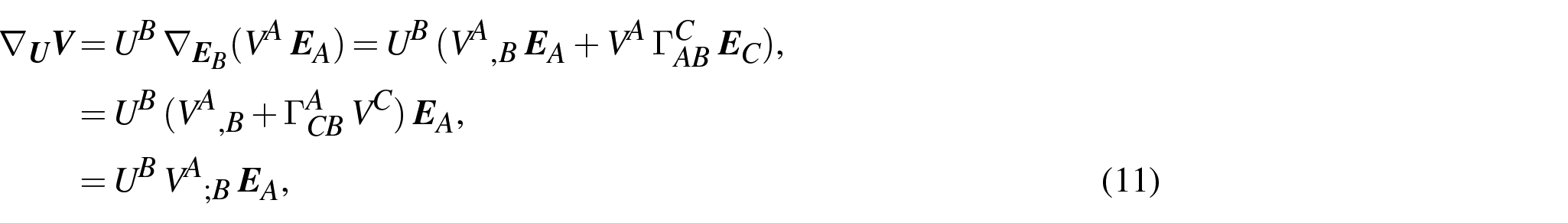
where

and the derivatives

are the covariant derivatives of the component
The torsion of the connection ∇ is defined as the third-order tensor

where the Lie bracket

In components, the torsion reads

and, when the torsion is zero, the Christoffel symbols are symmetric, i.e.,
2.3. Notable fourth-order tensors
This section presents a set of fourth-order tensors employed extensively within the theory of elasticity. These tensors are instrumental in the decomposition of symmetric second-order tensors into their spherical and deviatoric parts. Notably, certain forms of these tensors arise from the differentiation of the right Cauchy–Green deformation tensor
The pulled-back mixed symmetric identity


where
By raising all indices of the pulled-back operators (17) with the pull-back inverse metric tensor


and by lowering all indices with the pull-back metric tensor


Contracting the contravariant tensors (18) and the covariant tensors (19), we obtain the identities


Finally, we report the important results [77,79]


2.4. Equations of electrostatics
The formulation of electrostatics draws extensively from the established literature [27–29]. In the absence of volumetric densities of electric charges (no free charges in the interior of a dielectric) and in quasi-static conditions (negligible time derivatives of the fields), Maxwell’s equations reduce to the equations of electrostatics.
Let

where
Let

where
The local forms of the integral equations (22) and (23) are obtained by applying Gauss’ theorem and Stokes’ theorem, respectively. Together with the constitutive equation for the dielectric induction, these read


where the divergence and the curl operators are taken with respect to the spatial coordinates

is the constant dielectric permittivity tensor of vacuum, with
The material counterpart of equation (22) is obtained by performing the backward Piola transformation

where

where


where the material fields are related to the spatial fields by [22,25,84]


the divergence and the curl operators are taken with respect to the material coordinates

is the material dielectric permittivity tensor of vacuum. Note that, although the spatial dielectric permittivity tensor of vacuum
The spatial equation (24b) and the material equation (28b) imply that the electric field is obtained from the gradient of a scalar field, called electric potential or often just scalar potential, i.e.,


where

The spatial gradient of

Finally, we note that, on the boundary of the body, the dielectric induction must satisfy the condition


where

The factor of proportionality between
3. Material uniformity
A body
3.1. Definition of materially uniform body
A material body
This ‘fix’ is a linear map called material isomorphism, denoted
The archetype is like a blueprint for the material. For each point
Due to the definition of uniformity tensor
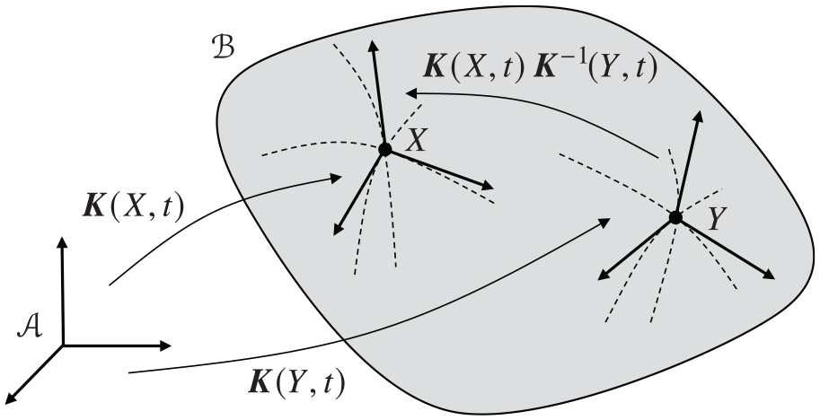
Representation of a materially uniform body
A vector field

where

where the

Comparison with equation (37) and the arbitrariness of

Note that, in the alternative expression
3.2. Uniform elastic dielectric body
Let us consider the definition of material uniformity provided in section 3.1. An elastic dielectric body is uniform if its Helmholtz free energy per unit reference volume, evaluated at a point

where
By defining the elastic (or archetypal) deformation, mapping from the archetype to the current configuration, and the archetypal electric field, respectively, as


we can write the energy density (40) as

Figure 2 depicts two key mappings:
The uniformity tensor
The elastic deformation
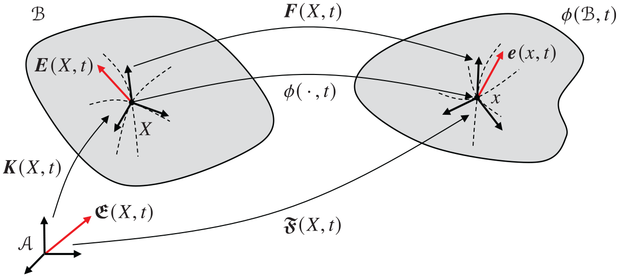
Mappings between the archetype
When we differentiate the free energy (42) with respect to


4. Governing equations
This section elucidates the governing equations for uniform non-linear electro-elastic solids. The formulation presented here treats the uniformity tensor
4.1. Principle of virtual work
Considering the motion


where
The principle of virtual work states that the internal virtual work
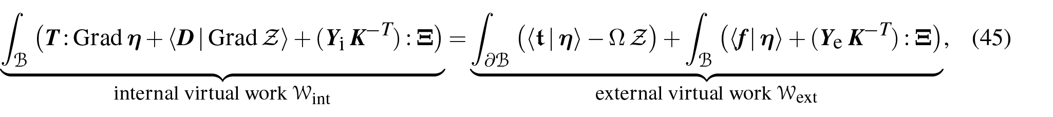
where the completely material tensors
Applying the divergence theorem to the surface integrals in equation (45), substituting the identities


in the first and second terms in the external virtual power


4.2. Dissipation inequality
In the isothermal case, the dissipation inequality reads [87,89,90]

Differentiating the referential energy density (42) with respect to time, we obtain
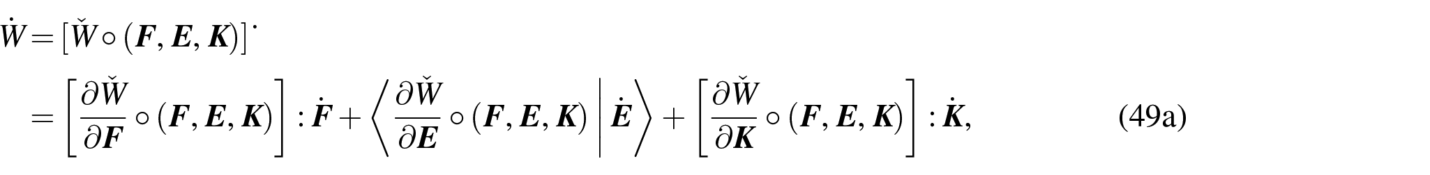
which, substituted in the dissipation inequality (48), gives
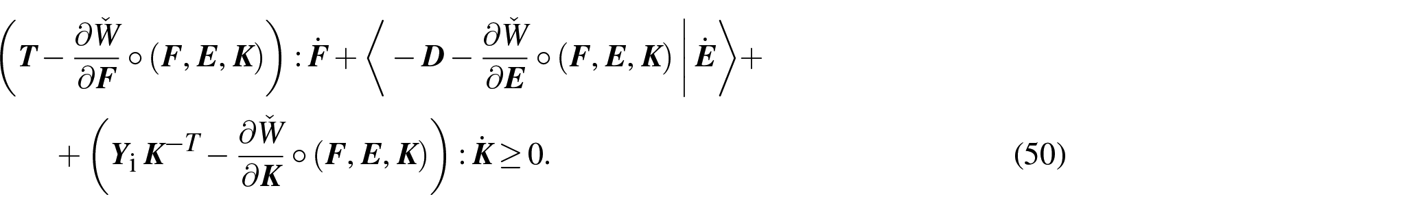
For the inequality (50) to be valid for any electromechanical process, it is necessary that, considering also equation (43),


The dissipation inequality (50) reduces to

and, using the definition

of inhomogeneity rate tensor, it can be written as

Let us consider the Helmholtz free density (42) and calculate the derivative with respect to the uniformity tensor

By exploiting equation (42) and the identities


arising from equation (51), we can put equation (55) in the form


By substituting equation (57) into the dissipation inequality (54), we arrive at

The negative of the Eshelby stress

the generalised force

where we used also equation (57). Therefore, if we write the total virtual work (45) by expressing the Piola stress
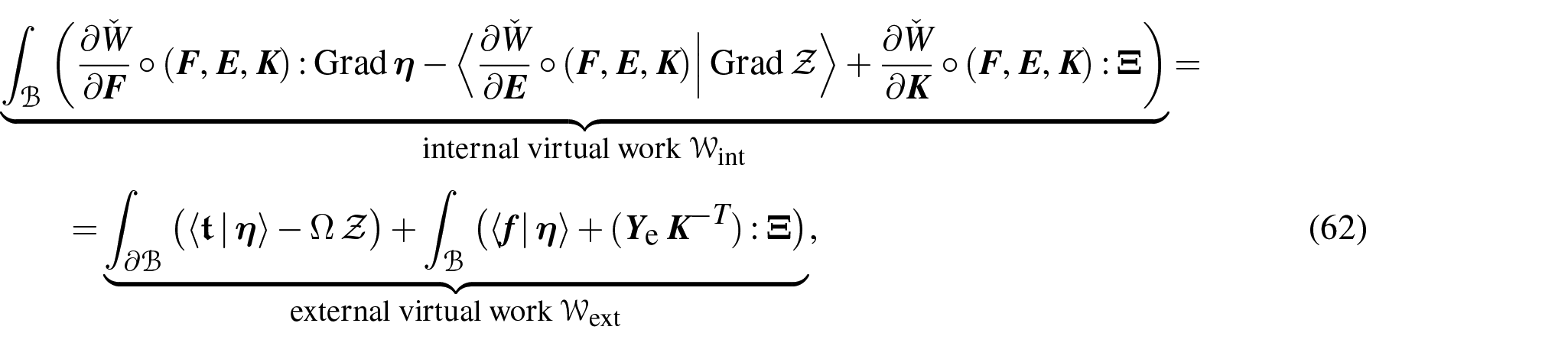
and consider the condition (61) of self-driven evolution, the principle of virtual work reduces to

i.e., it coincides with the case in which the uniformity tensor
Following the work by Elżanowski and Preston [98], we express the self-driven evolution law as in terms of the torsion Tor of the connection induced by the uniformity tensor

where

is the pull-back of the inhomogeneity rate tensor

4.3. Self-driven evolution law
Building on the work of Elżanowski and Preston [98], we introduce self-driven evolution laws based on the torsion
4.3.1. Diagonal case
In the diagonal case, the representing matrix of the uniformity tensor is, unsurprisingly, diagonal:
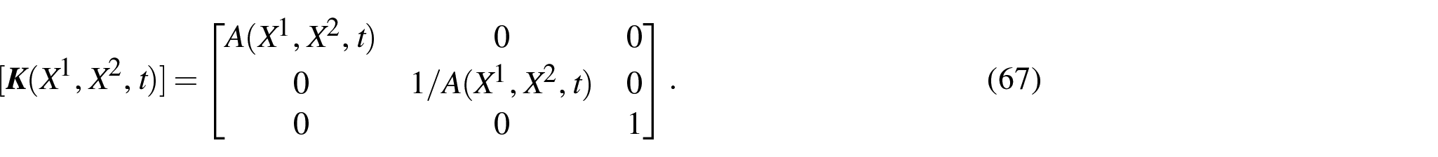
Substituting the uniformity tensor from equation (67) into the evolution law, which is formulated in terms of the torsion
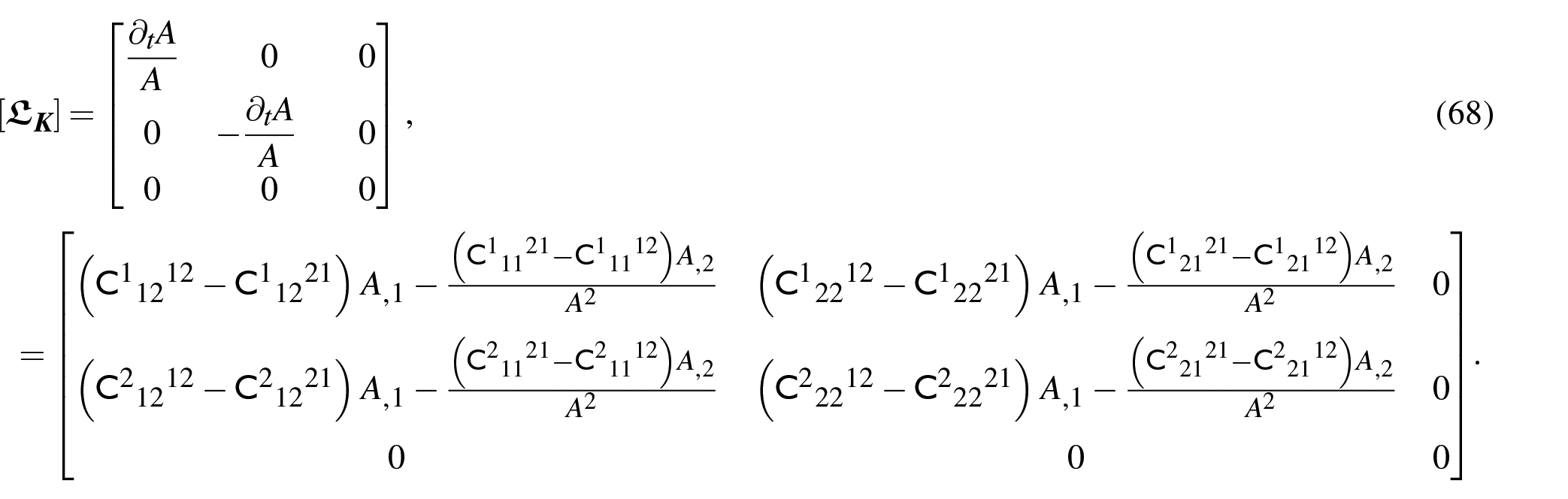
The archetypal velocity gradient


For equations (69b) and (69c) to be satisfied identically, it is necessary that


Applying the condition
For this condition to be satisfied identically, it is necessary that

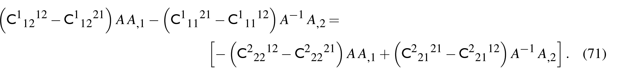
Therefore, by applying the relationships between the material constants, we derive a single partial differential equation for the scalar function

where

We solve the partial differential equation (74) using separation of variables and obtain the time-independent expression of

To ensure that
4.3.2. Nilpotent case
In the nilpotent case, the representing matrix of the uniformity tensor is upper-triangular:
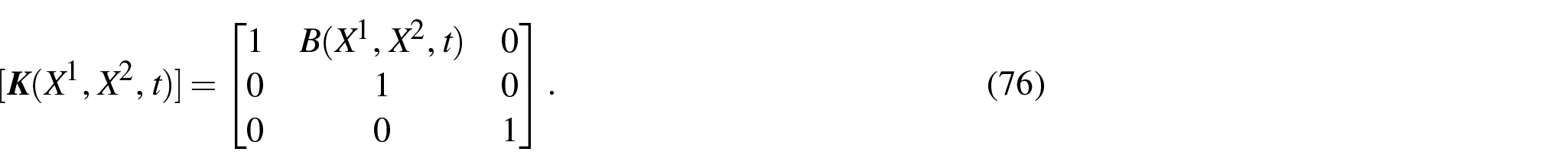
Substituting the uniformity tensor (76) into the evolution law (64) yields the matrix equation
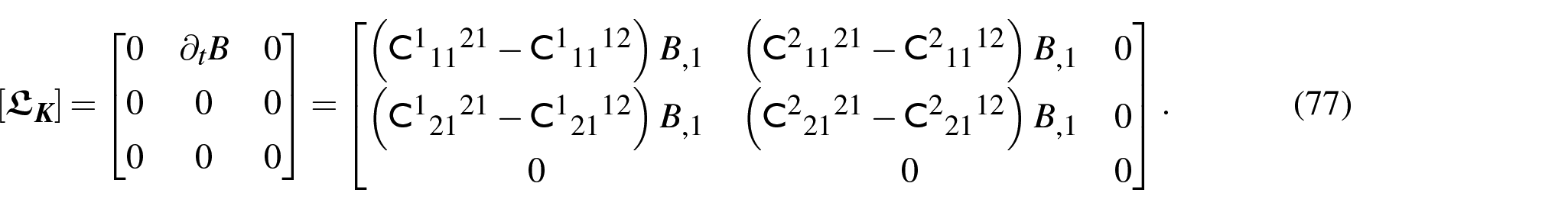
The archetypal velocity gradient


Conditions (78a), (78c) and (78d) yield


The only non-trivial partial differential equation is (78b) and reads

where we set

i.e.,

where
4.4. Finite element formulation
We consider a body


and, for the variations in motion


Incorporating these relationships into the principle of virtual work in the form equation (63), we arrive at a set of discrete equations, which can be linearised, by employing the Newton–Raphson iterative method, into
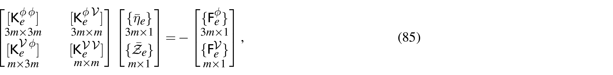
where we recall that

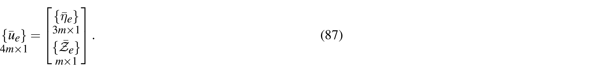
The vector
The local stiffness matrix


where


are the first elasticity tensor, the electro-elastic stiffness tensor and the dielectric permittivity tensor, respectively. The local vector of the nodal forces is given by the block vectors


where we recall that the first Piola–Kirchhoff stress
In equation (88), the double brackets
Mapping the pairs of indices
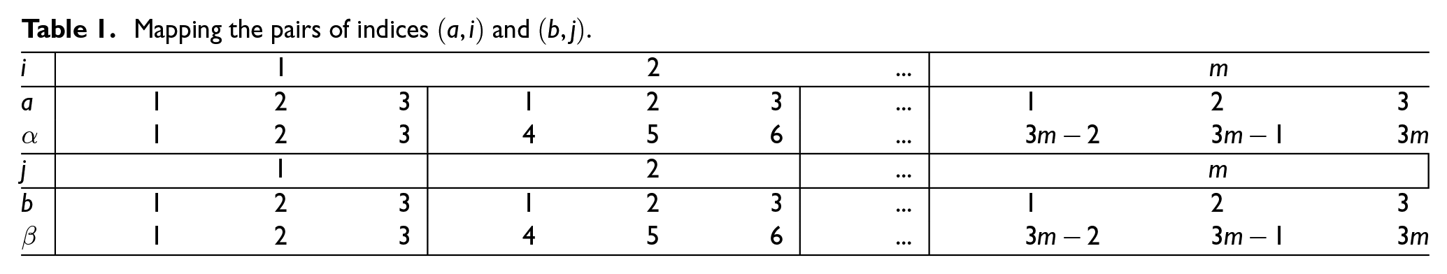
It is often convenient to express all quantities above in a local system of coordinates


The shape functions transform as

and their derivatives transform as


where the transformation matrices are clearly the inverse of each other:

Finally, the element-level equation (85) must be expanded to the global dimension
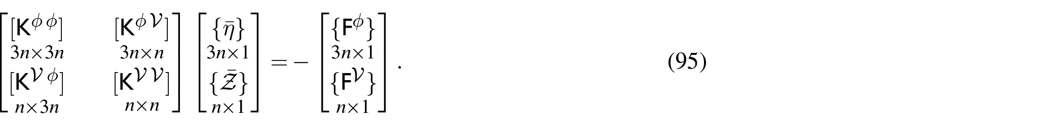
In compact form, we have

where
The system of equation (95) is iteratively solved for the increments in Lagrangian displacement field

This iterative process is repeated until the set convergence criterion is met.
4.5. Constitutive equations
We confine our attention to a nearly incompressible electrostrictive polyurethane with rubber-like properties [62], which undergoes large deformations.
The referential energy (42), which we report here for convenience,

must be frame-indifferent [67,101,102]. Frame-indifference requires that the referential constitutive functions

Indeed, the entirely material right Cauchy–Green tensor

As usually assumed in plasticity, we impose that the anelastic deformation described by the uniformity tensor

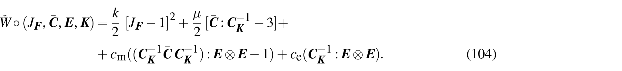
We adopt an energy similar to that in the paper by Ask et al. [62], which is written with the volumetric–distortional decomposition of

where

where
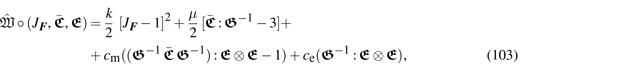
where the parameters
Following Federico [79], the second Piola–Kirchhoff stress

where

and, for the energy (103), they take the values

The first Piola–Kirchhoff stress

Thus, by substituting equation (105) into equation (108), the first Piola–Kirchhoff stress tensor

The material electric induction vector

The electromechanical tangent stiffness tensors, in the form used in the incremental equations (85) and (88) are written as a function of
We start from the second elasticity tensor

Since the energy (103) is decoupled in
where the fourth-order tensors

For the energy (103), the former reduces to the bulk modulus

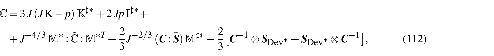
The first elasticity tensor [68] is obtained from the second as


The electro-elastic stiffness tensor is obtained most easily by differentiating the expression for


where we considered the symmetry of

5. Algorithm: finite element implementation in MATLAB
In this section, we describe a step-by-step guide for analysing dielectric elastomers with the finite element method on MATLAB. This tailored walkthrough focuses on the core computations for displacements and electric potential, and the iterative equation-solving with the Newton–Raphson method.
In the example problem that we study, we consider self-driven evolution, as described in section 4.3. Specifically, we examine two self-driven evolution laws: the diagonal case and the nilpotent case, both at steady state.
5.1. Initialisation
Set maximum Newton–Raphson iterations
Set the number of Gauss integration points
Initialise matrices for referential nodal coordinates.
Initialise assembly matrices (the matrices expanding from element dimension to global dimension).
5.2. Mesh construction and Gauss integration setup
Construct the connectivity array for hexahedral (brick-like) elements.
Define trilinear shape function
Construct the
Define the local coordinates
Define the weights
Set up boundary conditions.
Initialise
5.3. Loop for each Newton–Raphson iteration
5.3.1. Newton–Raphson loop
For each Newton–Raphson iteration (
Initialise
Loop over all elements (
■ Extract local node numbers and nodal values for
■ Initialise
■ Loop over Gauss points in all degrees of freedom:
□ Calculate shape functions
□ Convert shape function derivatives from parametric to physical coordinates, represented by
□ The matrix
□ Compute deformation gradient
□ Compute the first elasticity tensor
■ Assemble
Assemble
Apply boundary conditions to
Solve for
Check convergence: if error is below
5.3.2. Post-processing
Output the solution to a Tecplot ASCII file for visualisation
Display current iteration number and RMS (root mean square) error, calculated as part of the Newton–Raphson iterative process, as

where
Write the solution to separate files for visualisation in a software package such as VisIt (open source) or Tecplot (Bellevue, WA, USA)
5.3.3. Plot convergence history
Plot the RMS error against Newton–Raphson iterations
6. Numerical simulations
To evaluate the finite element implementation, we consider a beam-type actuator capable of bending in response to an applied electric field. The actuator is shown in Figure 3 and it comprises two perfectly bonded layers made of the same dielectric elastomer with identical material properties. The top layer is sandwiched between two (infinitely) compliant electrodes. Each layer has a thickness of
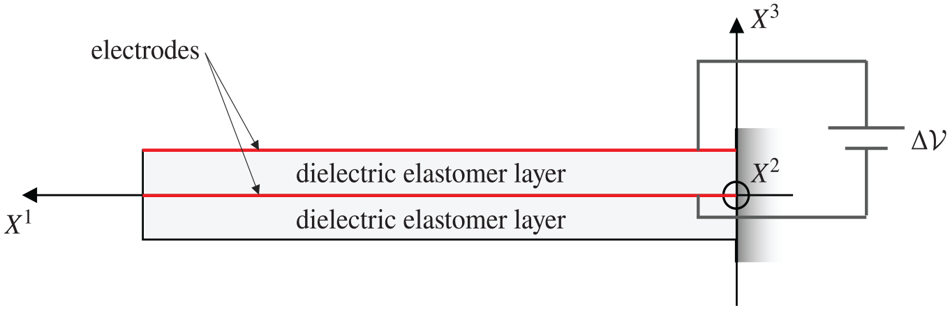
The bilayer dielectric elastomer beam of our example.
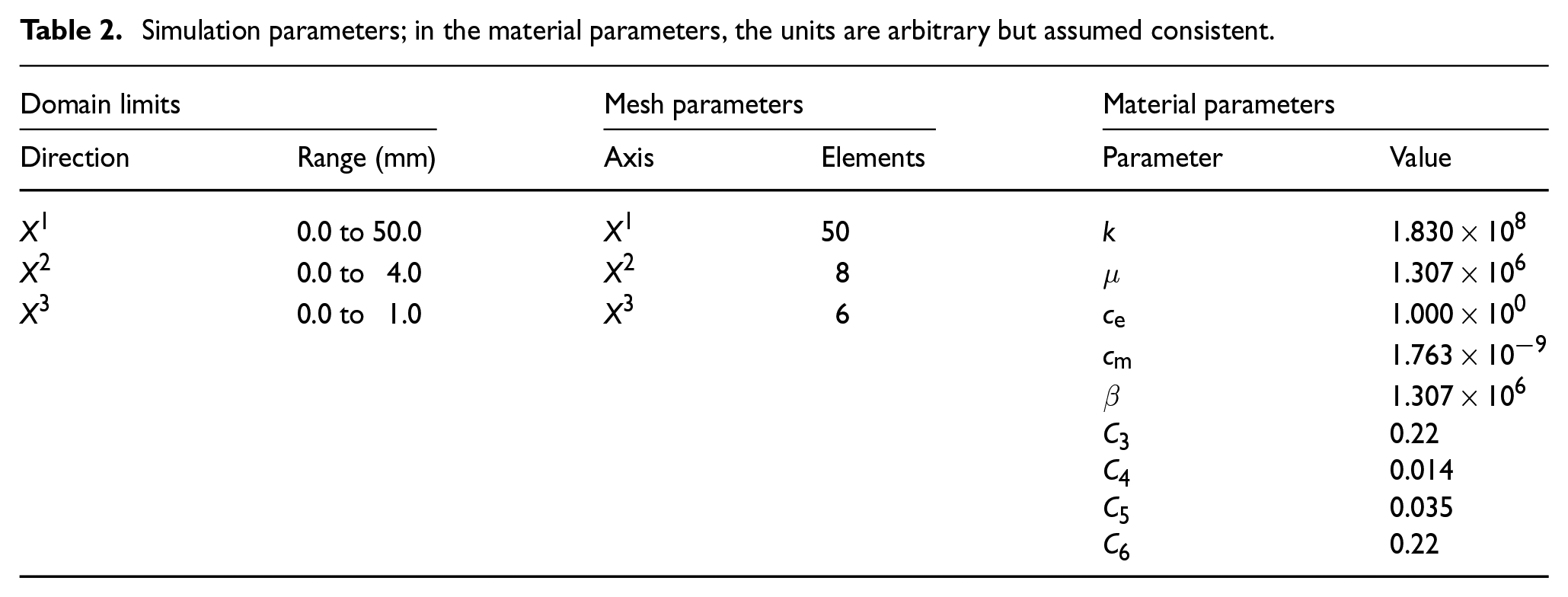
The mesh parameters, domain limits and material parameters (the units are arbitrary, but assumed consistent) are defined as in Table 2.
Simulation parameters; in the material parameters, the units are arbitrary but assumed consistent.
6.1. Case of homogeneous material
Let us first analyse the scenario in which
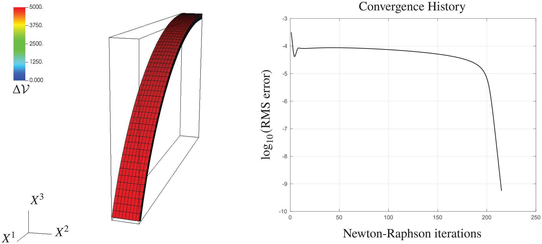
Deformation of a homogeneous beam under an applied electric field (left) and corresponding RMS error analysis (right).
6.2. Case of uniform material with self-driven evolution
Two distinct forms of the uniformity tensor
The left panel of Figure 5 shows the deformation in the case in which the uniformity tensor
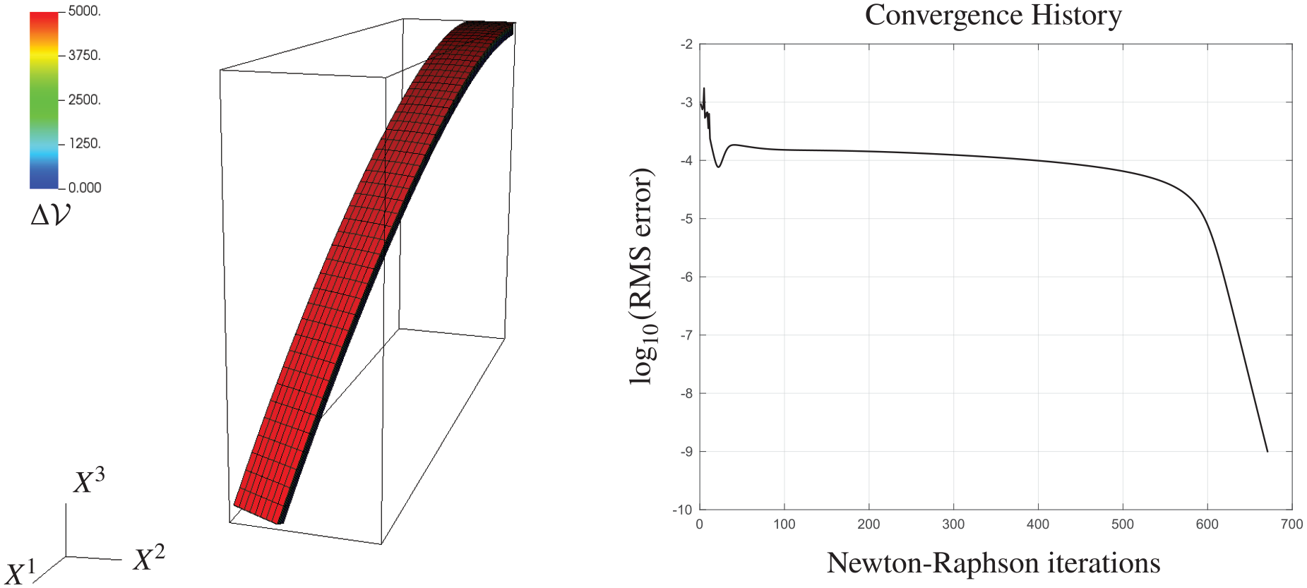
Warping caused by a diagonal uniformity tensor
The left panel of Figure 6 illustrates the case of nilpotent uniformity tensor
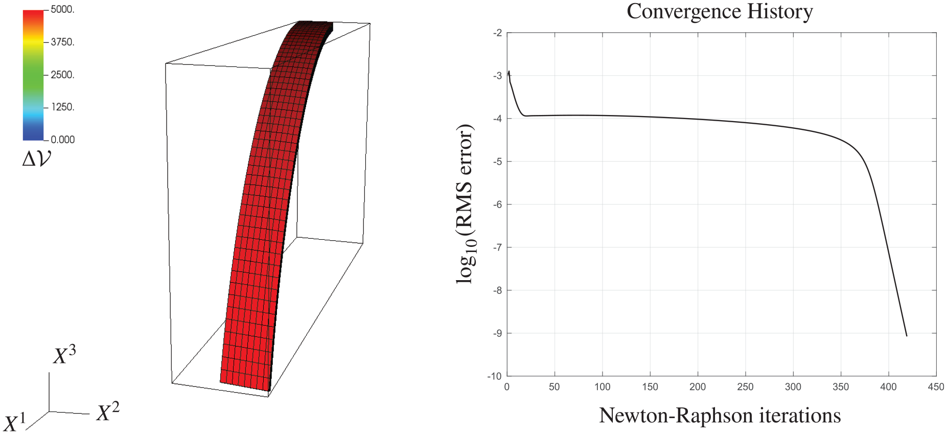
Warping caused by a nilpotent uniformity tensor
Figure 7 is a comparison of all cases studied: homogeneous (uncoloured meshed beam), diagonal and nilpotent. Both cases of nilpotent case,
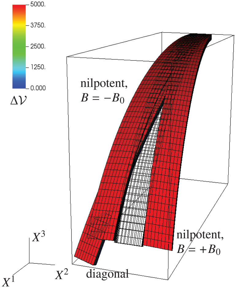
Comparison of the deformation of a homogeneous beam actuator (uncoloured mesh) with the deformation of beam actuators influenced by a diagonal or nilpotent uniformity tensor
7. Summary and outlook
In this study, we presented a model for uniform electro-elastic materials, in which we combined the theory of dielectric elastomers, rooted in the foundational works by Toupin [18–20] and others, the theory of material uniformity of Noll [4] in the formulation by Epstein and Maugin [5], and the theory of configurational mechanics of Eshelby [96,97], in the picture by Gurtin [85,86], Cermelli et al. [87] and DiCarlo and Quiligotti [88]. In this picture, the uniformity tensor
In our finite element implementation, we specifically selected a case where the uniformity tensor
A perfectly homogeneous beam;
A beam with a diagonal uniformity tensor, characterised by the function
A beam with a nilpotent uniformity tensor, characterised by the shear function
The diagonal case resulted in the beam bending and warping towards the left. The nilpotent case resulted in a different warping behaviour depending on the sign of the shear function
The analysis confirmed the convergence of the numerical solution in all scenarios and demonstrated the capability of our in-house finite element solver to accurately capture the complex interactions between electrical stimulation and material inhomogeneity in this type of actuator.
Our next steps shall be the study of two cases. The first consists in treating the uniformity tensor
Footnotes
Acknowledgements
We would like to thank Dr Alfio Grillo (Politecnico di Torino, Italy) for the important comments and suggestions on the constitutive framework.
Authors’ Note
Dedicated to Prof. Marcelo Epstein on occasion of his 80th birthday.
Dedication
This work is dedicated to our colleague, mentor and friend Prof. Marcelo Epstein. Marcelo has made fundamental contributions to the geometric theory of Continuum Mechanics and, in particular, to the theory of material uniformity. The influence that he and his work have had on our research and formation is immense. Through many years, Marcelo has always been a role model and a point of reference for all of us. Grazie, Marcelo.
Funding
The author(s) disclosed receipt of the following financial support for the research, authorship, and/or publication of this article: This work was supported in part by the Natural Sciences and Engineering Research Council of Canada, through the NSERC Alliance Programme, grant number ALLRP-571591-21 (S.F., Q.S.), and by Alberta Innovates (Canada), through the Advance Programme, grant number 212201535 (S.F., Q.S.).