Finite-strain Poynting–Thomson model: Existence and linearization

Abstract

We analyze the finite-strain Poynting–Thomson viscoelastic model. In its linearized small-deformation limit, this corresponds to the serial connection of an elastic spring and a Kelvin–Voigt viscoelastic element. In the finite-strain case, the total deformation of the body results from the composition of two maps, describing the deformation of the viscoelastic element and the elastic one, respectively. We prove the existence of suitably weak solutions by a time-discretization approach based on incremental minimization. Moreover, we prove a rigorous linx earization result, showing that the corresponding small-strain model is indeed recovered in the small-loading limit.

1. Introduction

Viscoelastic solids appear ubiquitously in applications. Polymers, rubber, biomaterials, wood, clay, and soft solids, including metals at close-to-melting temperatures, behave viscoelastically. The mechanical response of viscoelastic solids is governed by the interplay between elastic and viscous dynamics: by applying stresses, both strains and strain rates ensue [1]. This is on the basis of different effects, from viscoelastic creep, to viscous relaxation, to rate dependence in material response, and to dissipation of mechanical energy [2].

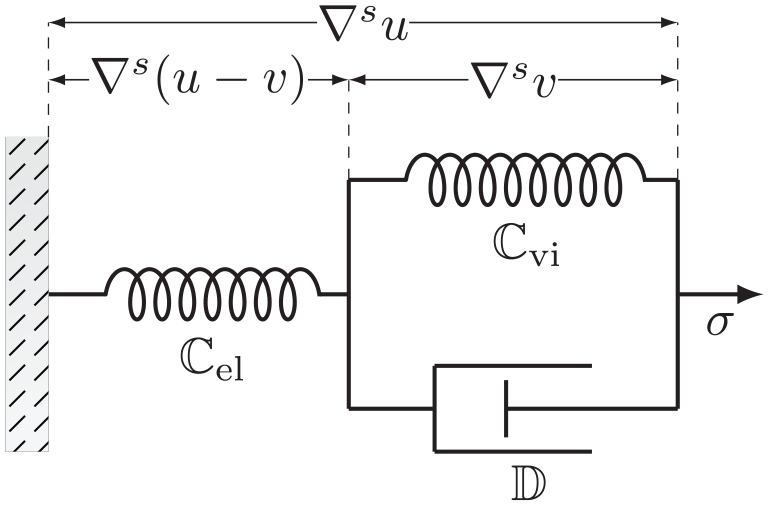
The modelization of viscoelastic solid response dates back to the early days of Continuum Mechanics. In the linearized, infinitesimal-strain setting of the standard-solid rheology, two basic models are the Maxwell and the Kelvin-Voigt, where an elastic spring is connected to a viscous dashpot in series or in parallel, respectively. These models offer only a simplified description of actual viscoelastic behavior. More accurate descriptions necessarily call for more complex models. The first option in this direction is the Poynting–Thomson model, resulting from the combination in series of an elastic and a Kelvin–Voigt component (see Figure 1). The second option would be the Zener model, which consists of an elastic and a Maxwell element in parallel. Note, however, that Poynting–Thomson and Zener can be proved to be equivalent in the linearized setting (see Kruzík, M and Roubíček [3, Remark 6.5.4]).

Figure 1.

The Poynting–Thomson rheological model (linearized setting).

The aim of this paper is to investigate the Poynting–Thomson model in the finite-strain setting. From the modeling viewpoint, extending the model beyond the small-strain case is crucial, for viscoelastic materials commonly experience large deformations. In fact, finite-strain versions of the Poynting–Thomson model have already been considered. The reader is referred to Lectez and Verron [4], where a comparison between Poynting–Thomson and Zener models at finite strains is discussed and to Meo et al. [5], focusing on the anisothermal version the Poynting–Thomson model.

To the best of our knowledge, mathematical results on the finite-strain Poynting–Thomson model are still not available. The focus of this paper is to fill this gap by presenting:

• an existence theory for solutions of the finite-strain Poynting–Thomson model, as well as a convergence result for time-discretizations (Theorem 4.1);

• a rigorous linearization result, proving that finite-strain solutions converge (up to subsequences) to solutions of the linearized system in the limit of small loadings and, correspondingly, small strains (Theorem 4.2).

Our analysis is variational in nature. The convergence result provides a rigorous counterpart to the classical heuristic arguments based on the Taylor expansions [4].

We postpone to section 2 both the detailed discussion of the model and a first presentation of our main results. We anticipate, however, here that the theory requires no second-gradient terms but rather relies on a decomposition of the total deformation in terms of an elastic and a viscous deformation (see equation (3)). Correspondingly, the variational formulation of the problem features both Lagrangian and Eulerian terms. Note, moreover, that the viscous dissipation is here assumed to be $p_{\psi }$ -homogeneous, with superlinear homogeneity $p_{\psi }\ge 2$ .

Our notion of solution (see Definition 4.1) hinges on the validity of an energy inequality, an elastic semistability inequality, and an approximability property via time-discrete problems. Albeit very weak, this notion replicates the important features of viscoelastic evolution, including elastic equilibrium, energy dissipation, and viscous relaxation.

Before moving on, let us put our results in context with respect to the available literature. In the purely partial differential equation (PDE) setting, existence results for viscoelastic dissipative systems are classical. The reader is referred to the recent monograph [3] for a comprehensive collection of references. As it is well known, the PDE setting is local in nature and, as such, does not allow considering global constraints such as injectivity of deformations, i.e., noninterpenetration of matter. Variational theories for viscoelastic evolution offer a remedy in this respect. Using the underlying gradient-flow structure of viscoelastic evolution, existence results for variational solutions have been obtained in the one-dimensional [6] and in the multi-dimensional case [7]. The latter paper also delivers a rigorous evolutive $\mathrm{\Gamma }$ -convergence linearization result (see also Krömer and Roubíček [8] for the case of self-contact and Badal et al. [9] and Mielke and Roubíˇcek [10] for some extension to nonisothermal situations). With respect to these contributions, we deal here with an internal-variable formulation, where the elastic variable does not dissipate. From the technical viewpoint, the novelty of our approach resides in avoiding the second-gradient theory by virtue of the composition assumption (3). This impacts on the functional setting, as well as on the required mathematical techniques.

In the different but related frame of activated inelastic deformations, the closest contributions to ours are Mielke et al. [11] and Röger and Schweizer [12], both dealing with rate-dependent viscoplasticity $(p_{\psi }>1)$ under the multiplicative-decomposition setting. In both papers, the existence of solutions is discussed, by taking into account additional gradient-type terms for the viscous strain. In particular, the full gradient is considered in Mielke et al. [11], whereas in Röger and Schweizer [12] only its curl is penalized. The approach in Röger and Schweizer [12] analogous to ours in terms of solution notion, despite the differences in the model. In contrast with these papers, viscous evolution is here not activated. In addition, by not considering here additional gradient terms, we avoid introducing a second length scale in the model and thus tackle so-called simple materials. Moreover, we investigate here linearization, which was not discussed in Mielke et al. [11] and Röger and Schweizer [12].

In the fully rate-independent setting $p_{\psi }=1$ of activated elastoplasticity, the papers Kruzík et al. [13], Stefanelli [14] and Mielke and Stefanelli [15], contribute an existence and linearization theory which is parallel the current viscoelastic one. More precisely, Kruzík et al. [13] and Stefanelli [14] deal with a decomposition of deformations in the same spirit of equation (3), avoiding the use of second gradients, whereas Mielke and Stefanelli [15] features no gradients, but it is a pure convergence result, in a setting where existence is not known. With respect to these contributions, the superlinear, nonactivated nature of the dissipation of the viscous setting calls for using a different set of analytical tools from gradient-flow theory [16]. Note that, also in the rate-independent setting, by including a gradient term of the plastic strain, hence resorting to so-called strain-gradient finite plasticity, one obtains stronger results. In particular, the existence of energetic solutions in strain-gradient finite plasticity is in Mainik and Mielke [17] and the linearization in some symmetrized case is in Grandi and Stefanelli [18]. Under the mere penalization of the curl of the gradient of the plastic strain, the existence of incremental solutions is proved in Mielke and Müller [19] and linearization is in Scala and Stefanelli [20].

This paper is organized as follows. In section 2, we provide an illustration of the finite-strain Poynting–Thomson model under consideration, as well as an introduction to our main results. Some preliminary material and comment on the functional setting is provided in section 3. In particular, we discuss the set of admissible deformations in section 3.2. In sections 4.1 and 4.3, we list and comment the assumptions, whereas the statements of our main results, Theorem 4.1 and Theorem 4.2 are presented in sections 4.2 and 4.4, respectively. The solvability of the time-discrete incremental problems is discussed in section 5, whereas the proofs of Theorems 4.1 and 4.2 are given in sections 6 and 7, respectively.

2. The finite-strain Poynting–Thomson model

In order to illustrate our results, we start by recalling the classical Poynting–Thomson in the linearized setting of infinitesimal strains. Indicating by $u:\mathrm{\Omega }\to {\mathbb{R}}^d$ the infinitesimal displacement from the reference configuration $\mathrm{\Omega }\subset {\mathbb{R}}^d$ , the total strain ${\nabla }^{s}u$ (here ${\nabla }^s$ denotes the symmetrized gradient ${\nabla }^{s}u=(\nabla u+\nabla u^{\top })/2$ ) is additively decomposed in its elastic and its viscous parts as ${\nabla }^{s}u={\mathbb{C}}_{\mathrm{el}}^{-1}\sigma +{\nabla }^{s}v$ . In its quasistatic approximation, the evolution of the body results from the combination of the equilibrium system and the constitutive relation, namely:

$$\begin{array}{c}-\mathrm{div}({\mathbb{C}}_{\mathrm{el}}{\nabla }^s(u-v))=f\mathrm{in}\mathrm{\Omega }\times (0,T),\hfill \\ \mathbb{D}{\nabla }^s\stackrel{·}{v}+({\mathbb{C}}_{\mathrm{vi}}+{\mathbb{C}}_{\mathrm{el}}){\nabla }^{s}v={\mathbb{C}}_{\mathrm{el}}{\nabla }^{s}u\mathrm{in}\mathrm{\Omega }\times (0,T),\hfill \end{array}$$

where $f$ stands for a given body force and $\stackrel{·}{v}$ denotes the time-derivative of $v$ . The reader is referred to the monographs [3, 21, 22] for a comprehensive collection of analytical results. Let us remark that in this paper, we will specifically consider the case of incompressible viscosity, i.e., in the linearized setting $\mathrm{tr}v=0$ . Hence, the evolution of the system considered is actually determined by the following equations:

$$-\mathrm{div}({\mathbb{C}}_{\mathrm{el}}{\nabla }^s(u-v))=f\mathrm{in}\mathrm{\Omega }\times (0,T),$$

(1)

$$\mathbb{D}{\nabla }^s\stackrel{·}{v}+({\mathbb{C}}_{\mathrm{vi}}+{\mathbb{C}}_{\mathrm{el}}){\nabla }^{s}v=\mathrm{dev}({\mathbb{C}}_{\mathrm{el}}{\nabla }^{s}u)\mathrm{in}\mathrm{\Omega }\times (0,T),$$

(2)

where $\mathrm{dev}$ denotes the deviatoric part of a tensor. Restricting to the incompressible case would call for accordingly specifying the rheological diagram from Figure 1 by distinguishing the volumetric and the deviatoric components.

In the finite-strain Poynting–Thomson model [4, 5], the state of the viscoelastic system is specified in terms of its deformation $y:\mathrm{\Omega }\to {\mathbb{R}}^d$ . As it is common in finite-strain theories [23], the deformation gradient $\nabla y$ is multiplicatively decomposed as $\nabla y=F_{\mathrm{el}}{F}_{\mathrm{vi}},$ where $F_{\mathrm{el}}$ and $F_{\mathrm{vi}}$ are the elastic and viscous strain tensors, representing the elastic and viscous response of the medium, respectively.

A distinctive feature of our approach is that we assume the viscous strain to be compatible: we identify $F_{\mathrm{vi}}$ with the gradient $\nabla y_{\mathrm{vi}}$ of a viscous deformation $y_{\mathrm{vi}}:\mathrm{\Omega }\to y_{\mathrm{vi}}(\mathrm{\Omega })\subset {\mathbb{R}}^d$ , mapping the reference configuration $\mathrm{\Omega }$ to the intermediate one $y_{\mathrm{vi}}(\mathrm{\Omega })$ . Correspondingly, the elastic strain is compatible as well and there exists an elastic deformation $y_{\mathrm{el}}:y_{\mathrm{vi}}(\mathrm{\Omega })\to {\mathbb{R}}^d$ , with $F_{\mathrm{el}}=\nabla y_{\mathrm{el}}$ mapping the intermediate configuration to the actual one. As such, the multiplicative decomposition $\nabla y=F_{\mathrm{el}}{F}_{\mathrm{vi}}$ ensues from an application of the classical chain rule to the composition:

$$y:=y_{\mathrm{el}}°y_{\mathrm{vi}}:\mathrm{\Omega }\to {\mathbb{R}}^d.$$

(3)

Moving from this position, the state of the medium is described by the pair $(y_{\mathrm{vi}},y_{\mathrm{el}})$ , effectively distinguishing viscous and elastic responses.

Before moving on, let us stress that the compatibility assumption on $F_{\mathrm{vi}}$ , whence the composition assumption (3), realistically describes a variety of viscoelastic evolution settings and refer to Kruzík et al. [13] and Stefanelli [14] for some parallel theory in the frame of finite-strain plasticity. In particular, position (3) is flexible enough to cover both limiting cases of a purely elastic $(y_{\mathrm{vi}}=\mathrm{id})$ and of a plain Kelvin–Voigt $(y_{\mathrm{el}}=\mathrm{id})$ materials. In the linearized setting, these would formally correspond to the cases ${\mathbb{C}}_{\mathrm{vi}}\to \infty$ and ${\mathbb{C}}_{\mathrm{el}}\to \infty$ , respectively. Let us note that by choosing ${\mathbb{C}}_{\mathrm{vi}}=0$ , the linearized systems (1) and (2) reduces to the Maxwell fluidic rheological model. By assuming equation (3), we exclude the onset of defects, such as dislocations and disclinations. Albeit this could limit the application of the theory in some specific cases, it is to remark that viscous materials are often amorphous, so that the relevance of strictly crystallographic descriptions may be questionable. From the more analytical viewpoint, assumption (3) allows us to present a comprehensive mathematical theory within the setting of so-called simple materials, i.e., without resorting to second-gradient theories. The alternative path of including second-order deformation gradients, is also viable and, as far as existence is concerned, has been considered in Mielke et al. [11] in the activated case of viscoplasticity.

A first consequence of the composition (3) is that the elastic deformation $y_{\mathrm{el}}$ is defined on the a priori unknown intermediate configuration $y_{\mathrm{vi}}(\mathrm{\Omega })$ , making the analysis delicate. In particular, the variational description of the viscoelastic behavior results in a mixed Lagrangian–Eulerian variational problem. This mixed nature of the problem will be tamed by means of change-of-variables techniques, which in turn ask for some specification on the class of admissible intermediate configurations. Let us anticipate that $y_{\mathrm{vi}}$ will be required to be an incompressible $(det\nabla y_{\mathrm{vi}}=1)$ homeomorphism throughout. We refer to Haupt and Lion [24] and Wijaya et al. [25] for models of incompressible viscoelastic solids. As it is mentioned in Devedran and Peskin [26], incompressibility is a somewhat standard assumption in the setting of biological applications (see also Berjamin and Chockalingam [27] for modeling of brain tissues). Our interest in the incompressible case is also motivated by the prospects of devising a sound existence theory. Assuming incompressibility has the net effect of simplifying change-of-variable formulas, ultimately allowing the mathematical treatment.

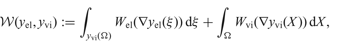
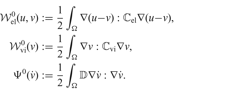
The stored energy of the medium is assumed to be of the form:

$$\mathcal{W}(y_{\mathrm{el}},y_{\mathrm{vi}}):={\int }_{y_{\mathrm{vi}}(\mathrm{\Omega })}{W}_{\mathrm{el}}(\nabla y_{\mathrm{el}}(\xi ))\mathrm{d}\xi +{\int }_{\mathrm{\Omega }}{W}_{\mathrm{vi}}(\nabla y_{\mathrm{vi}}(X))\mathrm{d}X.$$

(4)

Here and in the following, we indicate by $X$ the variable in the reference configuration $\mathrm{\Omega }$ and by $\xi$ the variable in the intermediate configuration $y_{\mathrm{vi}}(\mathrm{\Omega })$ . The first integral above corresponds to the stored elastic energy and the given function $W_{\mathrm{el}}$ is the stored elastic energy density. Its argument $\nabla y_{\mathrm{el}}(\xi )$ can be equivalently rewritten in Lagrangian variables as the usual product $\nabla y(X)\nabla y_{\mathrm{vi}}^{-1}(X)$ . By comparing these two expressions, the advantage of working in Eulerian variables is apparent, for $\nabla y_{\mathrm{el}}(\xi )$ is linear in $y_{\mathrm{el}}$ . The function $W_{\mathrm{vi}}$ is the stored viscous energy density instead and the corresponding integral is Lagrangian.

The instantaneous dissipation of the system is given by:

$$\mathrm{\Psi }(y_{\mathrm{vi}},{\stackrel{·}{y}}_{\mathrm{vi}}):={\int }_{\mathrm{\Omega }}\psi (\nabla {\stackrel{·}{y}}_{\mathrm{vi}}(\nabla y_{\mathrm{vi}}{)}^{-1})\mathrm{d}X,$$

(5)

where $\psi (·)$ models the instantaneous dissipation density and is assumed to be $p_{\psi }$ -positively homogeneous for $p_{\psi }\ge 2$ .

By formally taking variations of the above introduced functionals, we obtain the quasistatic equilibrium system [28]:

$$\begin{array}{c}-\mathrm{div}\mathrm{D}{W}_{\mathrm{el}}(\nabla y_{\mathrm{el}})=f°y_{\mathrm{vi}}^{-1}\mathrm{in}{y}_{\mathrm{vi}}(\mathrm{\Omega })\times (0,T)\hfill \\ \mathrm{D}{W}_{\mathrm{el}}(\nabla y_{\mathrm{el}}(y_{\mathrm{vi}}):{\mathrm{D}}^2{y}_{\mathrm{el}}(y_{\mathrm{vi}}))+\mathrm{div}\mathrm{D}{W}_{\mathrm{vi}}(\nabla y_{\mathrm{vi}})\hfill \\ -\nabla y_{\mathrm{el}}(y_{\mathrm{vi}}{)}^{\top }f=-\mathrm{div}\left(\mathrm{D}\psi {(\nabla {\stackrel{·}{y}}_{\mathrm{vi}}(\nabla y_{\mathrm{vi}}))}^{-1}\right)(\nabla y_{\mathrm{vi}}{)}^{-\top })\mathrm{in}\mathrm{\Omega }\times (0,T).\hfill \end{array}$$

The highly nonlinear character of this system, combined with the absence of higher-order gradients in the viscous variable, forces us to consider a suitable weak-solution notion.

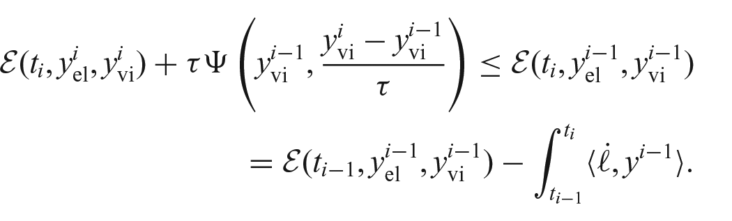
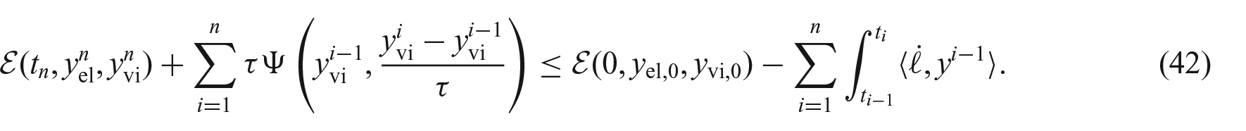
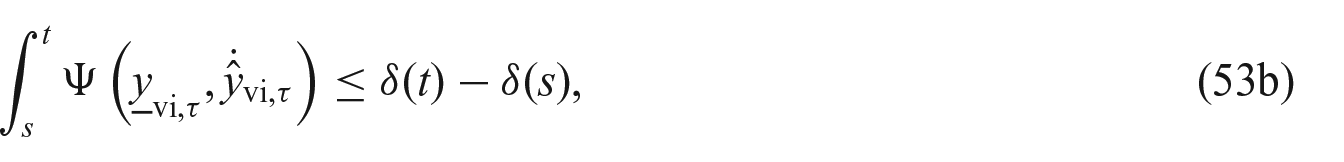
Inspired by Maso and Lazzaroni [29, Definition 2.12] and Röger and Schweizer [12, Definition 2.2], in our first main result, Theorem 4.1, we prove the existence of approximable solutions (see Definition 4.1). These are everywhere defined trajectories $(y_{\mathrm{el}},y_{\mathrm{vi}}):[0,T]\to W^{1,p_{\mathrm{el}}}(y_{\mathrm{vi}}(\mathrm{\Omega });{\mathbb{R}}^d)\times W^{1,p_{\mathrm{vi}}}(\mathrm{\Omega };{\mathbb{R}}^d)$ starting from some given initial datum $(y_{\mathrm{el},0},y_{\mathrm{vi},0})$ and satisfying for all $t\in [0,T]$ :

$\mathrm{Energy}\mathrm{in}\mathrm{equality}:$

$$\begin{array}{c}{\int }_{y_{\mathrm{vi}}(t,\mathrm{\Omega })}{W}_{\mathrm{el}}(\nabla y_{\mathrm{el}}(t,\xi ))\mathrm{d}\xi +{\int }_{\mathrm{\Omega }}{W}_{\mathrm{vi}}(\nabla y_{\mathrm{vi}}(t,X))\mathrm{d}X-{\int }_{\mathrm{\Omega }}f(t,X)·y_{\mathrm{el}}(t,y_{\mathrm{vi}}(t,X))\mathrm{d}X\hfill \\ +p_{\psi }{\int }_0^t{\int }_{\mathrm{\Omega }}\psi (\nabla {\stackrel{·}{y}}_{\mathrm{vi}}(s,X)(\nabla y_{\mathrm{vi}}(s,X){)}^{-1})\mathrm{d}X\mathrm{d}s\hfill \\ \le {\int }_{y_{\mathrm{vi},0}(\mathrm{\Omega })}{W}_{\mathrm{el}}(\nabla y_{\mathrm{el},0}(\xi ))\mathrm{d}\xi +{\int }_{\mathrm{\Omega }}{W}_{\mathrm{vi}}(\nabla y_{\mathrm{vi},0}(X))\mathrm{d}X-{\int }_{\mathrm{\Omega }}f(0,X)·y_{\mathrm{el},0}(y_{\mathrm{vi},0}(X))\mathrm{d}X\hfill \\ -{\int }_0^t{\int }_{\mathrm{\Omega }}{\partial }_{s}f(s,X)·y_{\mathrm{el}}(s,y_{\mathrm{vi}}(s,X))\mathrm{d}X\mathrm{d}s.\hfill \end{array}$$

(6)

$\mathrm{Semistability}\mathrm{condition}:$

$$\begin{array}{c}{\int }_{y_{\mathrm{vi}}(t,\mathrm{\Omega })}{W}_{\mathrm{el}}(\nabla y_{\mathrm{el}}(t,\xi ))\mathrm{d}\xi -{\int }_{\mathrm{\Omega }}f(t,X)·y_{\mathrm{el}}(t,y_{\mathrm{vi}}(t,X))\mathrm{dX}\hfill \\ \le {\int }_{y_{\mathrm{vi}}(t,\mathrm{\Omega })}{W}_{\mathrm{el}}(\nabla {\tilde{y}}_{\mathrm{el}}(\xi ))\mathrm{d}\xi -{\int }_{\mathrm{\Omega }}f(t,X)·{\tilde{y}}_{\mathrm{el}}(y_{\mathrm{vi}}(t,X))\mathrm{dX}\hfill \\ \forall {\tilde{y}}_{\mathrm{el}}\mathrm{with}({\tilde{y}}_{\mathrm{el}},y_{\mathrm{vi}}(t,·))\in \mathcal{A},\hfill \end{array}$$

(7)

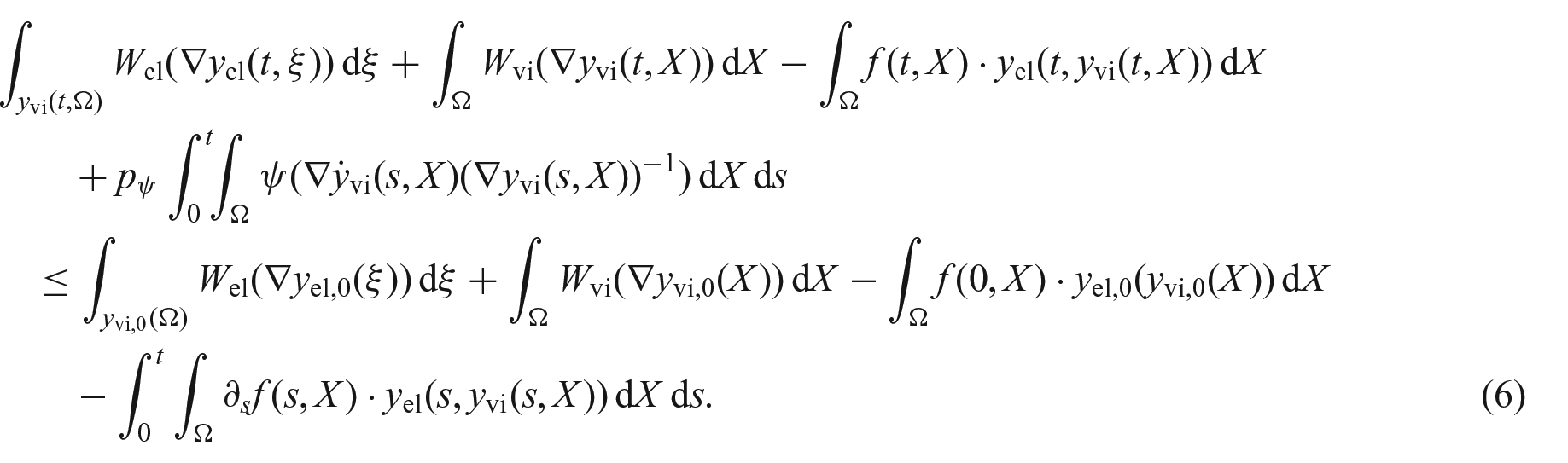
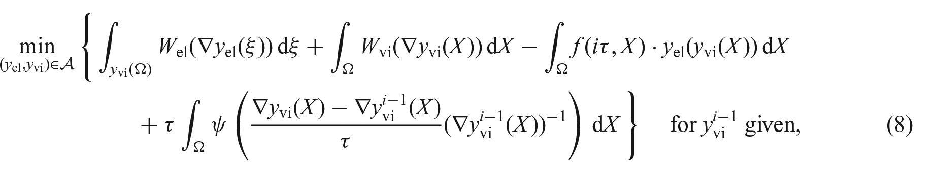
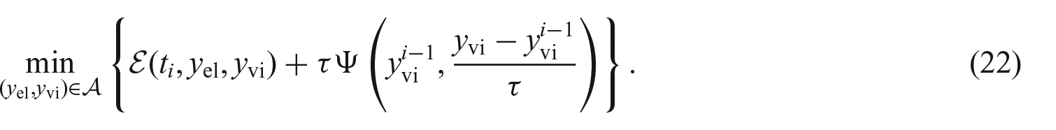
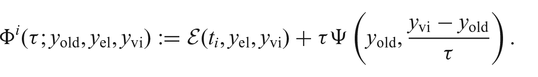
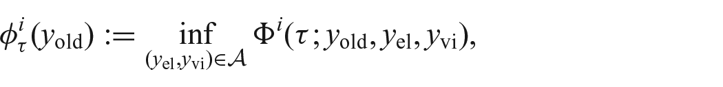
where $\mathcal{A}$ is the set of admissible deformations, introduced in section 3.2. The first line of inequality (6) corresponds to the total energy of the medium at time $t$ and state $(y_{\mathrm{el}}(t,·),y_{\mathrm{vi}}(t,·))$ . In particular, the term $-{\int }_{\mathrm{\Omega }}f·(y_{\mathrm{el}}°y_{\mathrm{vi}})\mathrm{dX}$ is the work of the (external) force $f$ (later, a boundary traction will be considered, as well). Solutions $t\mapsto (y_{\mathrm{el}}(t),y_{\mathrm{vi}}(t))$ are, moreover, required to be approximable, namely, to ensue as limit of time discretizations. In this respect, we consider the incremental minimization problems, for $i=1,\dots ,N$ ,

$$\begin{array}{c}\underset{(y_{\mathrm{el}},y_{\mathrm{vi}})\in \mathcal{A}}{min}\{{\int }_{y_{\mathrm{vi}}(\mathrm{\Omega })}{W}_{\mathrm{el}}(\nabla y_{\mathrm{el}}(\xi ))\mathrm{d}\xi +{\int }_{\mathrm{\Omega }}{W}_{\mathrm{vi}}(\nabla y_{\mathrm{vi}}(X))\mathrm{d}X-{\int }_{\mathrm{\Omega }}f(i\tau ,X)·y_{\mathrm{el}}(y_{\mathrm{vi}}(X))\mathrm{d}X\hfill \\ +\tau {\int }_{\mathrm{\Omega }}\psi \left(\frac{\nabla y_{\mathrm{vi}}(X)-\nabla y_{\mathrm{vi}}^{i-1}(X)}{\tau }{(\nabla y_{\mathrm{vi}}^{i-1}(X))}^{-1}\right)\mathrm{d}X\}\mathrm{for}{y}_{\mathrm{vi}}^{i-1}\mathrm{given},\hfill \end{array}$$

(8)

on a given uniform time-partition $\{0=t_0<t_1<\dots <t_N=T\}$ , where the set of admissible states $\mathcal{A}$ is defined in section 3.2.

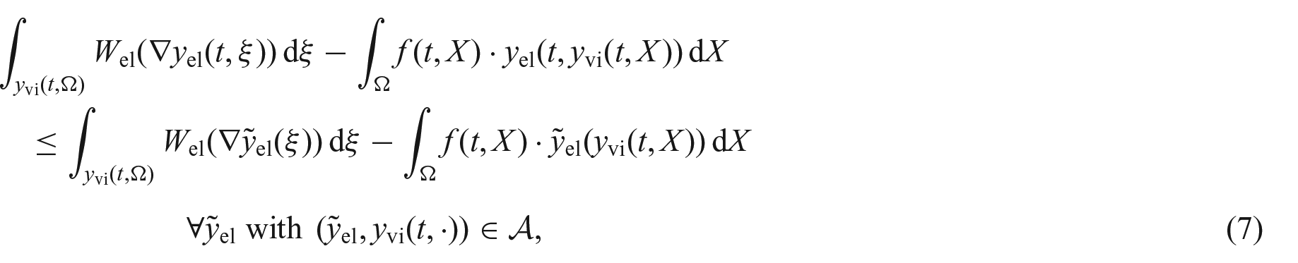
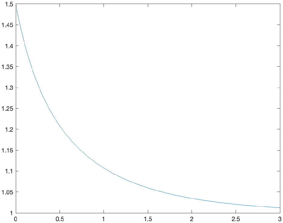
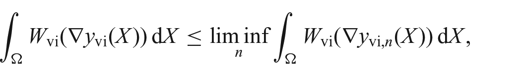
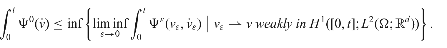
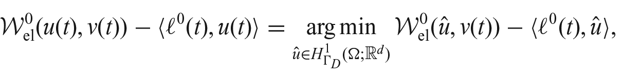
The notion of approximable solution is capable of reproducing the main features of viscoelastic evolution. First, the semistability condition (7) implies that $y_{\mathrm{el}}$ solves the elastic equilibrium at all times, given the viscous-state evolution. Correspondingly, the description of the purely elastic response of the material is complete. Second, the energy inequality (6) is sharp, in the sense that it may indeed hold as equality in specific smooth situations. In other words, all dissipative contributions are correctly taken into account in equation (6). Note in this respect the presence of the factor $p_{\psi }$ multiplies the dissipation term in equation (6). Eventually, the approximation property ensures that viscous evolution actually occurs, even in the absence of applied loads. We give an illustration of this fact in section 4.2 (see Figure 2).

Figure 2.

Evolution of the viscous strain $t\in [0,3]\to F_{\mathrm{vi}}(t)$ in the limit $\tau \to 0$ from problem (25), starting from $F_{\mathrm{vi}}^0=1.5$ .

Under suitable assumptions, the incremental minimization problems (8) are proved to admit solutions in Proposition 4.1. These time-discrete solutions fulfill a discrete energy inequality and a discrete semistability inequality. The existence of approximable solutions (Theorem 4.1) follows by passing to the limit in the time-discrete problems. In order to pass from the time-discrete to the time-continuous energy inequality (6), lower semicontinuity of the energy and dissipation functionals is necessary, which translates in our setting in asking for the polyconvexity of the respective densities. In order to obtain the specific form (6), we need to resort to the notion of De Giorgi variational interpolant [30, Definition 3.2.1, p. 66] and adapt this tool from its original metric-space application to the current one.

For establishing the elastic semistability (7), a suitable recovery-sequence construction is required. This calls for the extension of the elastic deformations from the intermediate configurations to the whole ${\mathbb{R}}^d$ . The possibility of performing this extension requires some regularity of the boundary of the intermediate configurations, which we ask to be Jones domains (see Definition 3.1).

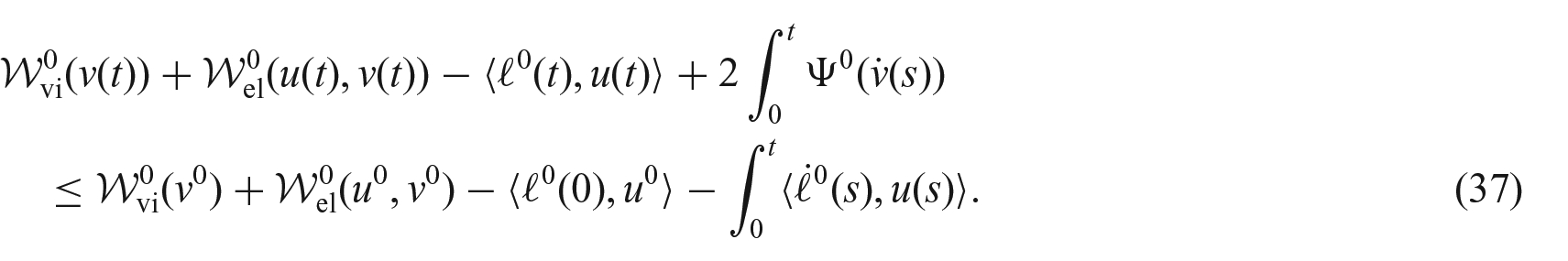
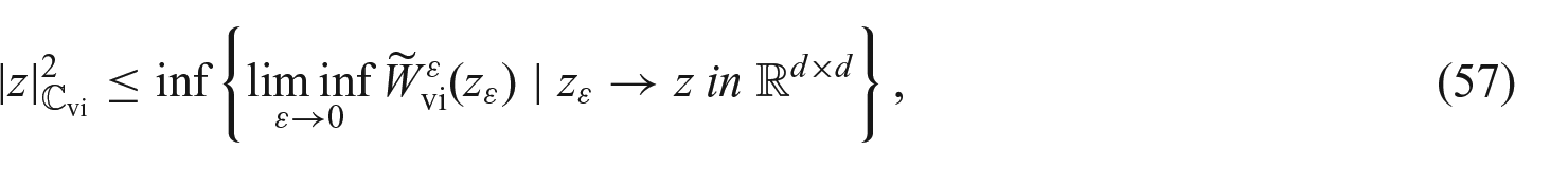
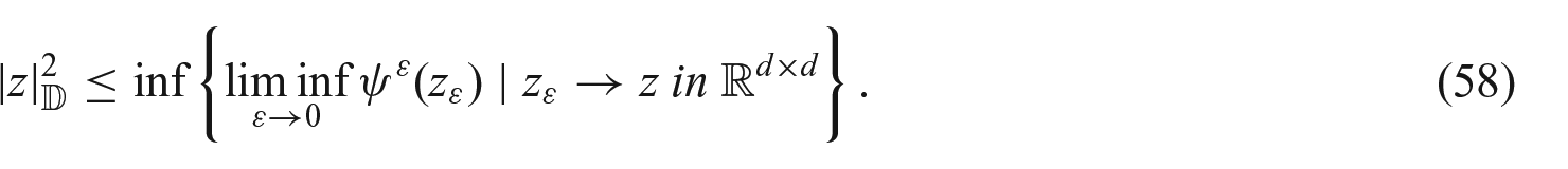
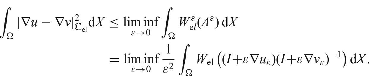
The second main focus of this paper is on the rigorous linearization of the system through evolutionary $\mathrm{\Gamma }$ -convergence [31] in the case of quadratic dissipations, namely, for $p_{\psi }=2$ . Moving from the seminal paper [32] in the stationary, hyperelastic case, the application of $\mathrm{\Gamma }$ -convergence to inelastic evolutive problems has been started in Mielke and Stefanelli [15] and has been applied to different settings. In particular, linearization in the incompressible case has been discussed in Jesenko and Schmidt [33], Mainini and Percivale [34, 35]. The goal is to provide a rigorous formalization of heuristic Taylor expansion arguments which, for the finite-strain Poynting–Thomson model, were already presented in Lectez and Verron [4]. At first, let us review this heuristic by assuming sufficient regularity of all ingredients.

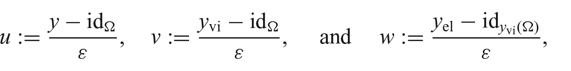
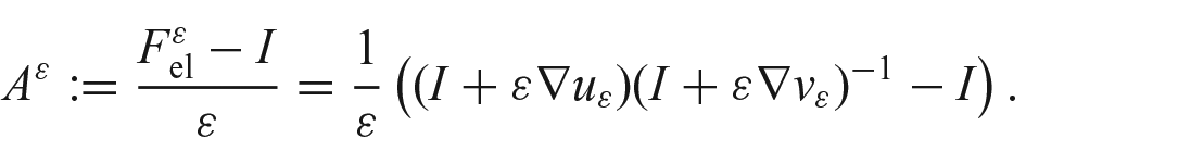
Consider the functions $u,v,w$ defined as:

$$u:=\frac{y-\mathrm{i}{\mathrm{d}}_{\mathrm{\Omega }}}{\epsilon },v:=\frac{y_{\mathrm{vi}}-\mathrm{i}{\mathrm{d}}_{\mathrm{\Omega }}}{\epsilon },\mathrm{and}w:=\frac{y_{\mathrm{el}}-\mathrm{i}{\mathrm{d}}_{y_{\mathrm{vi}}(\mathrm{\Omega })}}{\epsilon },$$

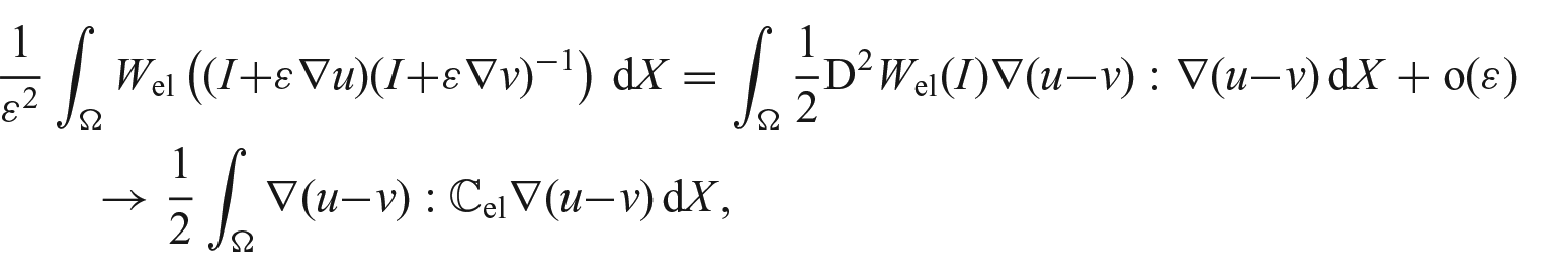
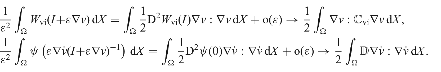
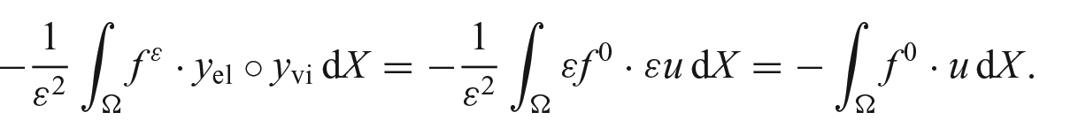
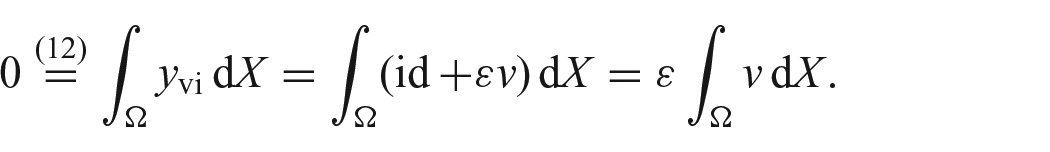
so that $u,v,w$ actually correspond to the $\epsilon$ -rescaled displacements of $y,y_{\mathrm{vi}},y_{\mathrm{el}}$ , respectively. To compute the linearization, it will be more convenient to work with the pair $(u,v)$ corresponding to the total and viscous deformations $(y,y_{\mathrm{vi}})$ . In particular, we replace $\nabla y=I+\epsilon \nabla u$ and $\nabla y_{\mathrm{vi}}=I+\epsilon \nabla v$ in the stored energy and $\nabla {\stackrel{·}{y}}_{\mathrm{vi}}=\epsilon \nabla \stackrel{·}{v}$ in the dissipation. By formally Taylor expanding the (rescaled) energy terms and taking $\epsilon \to 0$ , we find:

$$\begin{array}{c}\frac{1}{{\epsilon }^2}{\int }_{\mathrm{\Omega }}{W}_{\mathrm{el}}((I+\epsilon \nabla u)(I+\epsilon \nabla v{)}^{-1})\mathrm{d}X={\int }_{\mathrm{\Omega }}\frac{1}{2}{\mathrm{D}}^2{W}_{\mathrm{el}}(I)\nabla (u-v):\nabla (u-v)\mathrm{d}X+\mathrm{o}(\epsilon )\hfill \\ \to \frac{1}{2}{\int }_{\mathrm{\Omega }}\nabla (u-v):{\mathbb{C}}_{\mathrm{el}}\nabla (u-v)\mathrm{d}X,\hfill \end{array}$$

$$\begin{array}{c}\frac{1}{{\epsilon }^2}{\int }_{\mathrm{\Omega }}{W}_{\mathrm{vi}}(I+\epsilon \nabla v)\mathrm{d}X={\int }_{\mathrm{\Omega }}\frac{1}{2}{\mathrm{D}}^2{W}_{\mathrm{vi}}(I)\nabla v:\nabla v\mathrm{d}X+\mathrm{o}(\epsilon )\to \frac{1}{2}{\int }_{\mathrm{\Omega }}\nabla v:{\mathbb{C}}_{\mathrm{vi}}\nabla v\mathrm{d}X,\hfill \\ \frac{1}{{\epsilon }^2}{\int }_{\mathrm{\Omega }}\psi (\epsilon \nabla \stackrel{·}{v}{(I+\epsilon \nabla v)}^{-1})\mathrm{d}X={\int }_{\mathrm{\Omega }}\frac{1}{2}{\mathrm{D}}^2\psi (0)\nabla \stackrel{·}{v}:\nabla \stackrel{·}{v}\mathrm{d}X+\mathrm{o}(\epsilon )\to \frac{1}{2}{\int }_{\mathrm{\Omega }}\mathbb{D}\nabla \stackrel{·}{v}:\nabla \stackrel{·}{v}\mathrm{d}X.\hfill \end{array}$$

Here, we have assumed $W_{\mathrm{el}}(I)=W_{\mathrm{vi}}(I)=0$ , $\mathrm{D}{W}_{\mathrm{el}}(I)=\mathrm{D}{W}_{\mathrm{vi}}(I)=0$ , and have defined ${\mathbb{C}}_{\mathrm{el}}:={\mathrm{D}}^2{W}_{\mathrm{el}}(I)$ , ${\mathbb{C}}_{\mathrm{vi}}:={\mathrm{D}}^2{W}_{\mathrm{vi}}(I)$ , and $\mathbb{D}:={\mathrm{D}}^2\psi (0)$ . Moreover, we assume that the force $f$ is small, i.e., $f=f^{\epsilon }=\epsilon f^0$ . Hence, by neglecting the term $f^0·\mathrm{i}{\mathrm{d}}_{\mathrm{\Omega }}$ , which is independent of the displacement, the rescaled loading term reads:

$$-\frac{1}{{\epsilon }^2}{\int }_{\mathrm{\Omega }}{f}^{\epsilon }·y_{\mathrm{el}}°y_{\mathrm{vi}}\mathrm{d}X=-\frac{1}{{\epsilon }^2}{\int }_{\mathrm{\Omega }}\epsilon f^0·\epsilon u\mathrm{d}X=-{\int }_{\mathrm{\Omega }}{f}^0·u\mathrm{d}X.$$

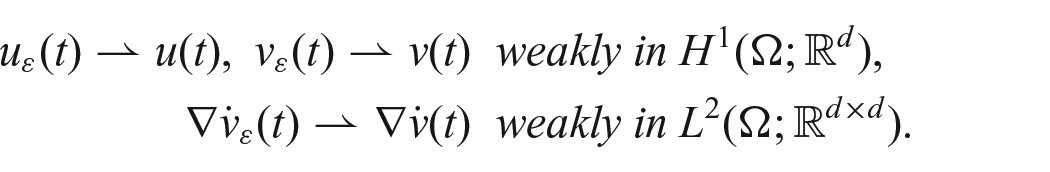
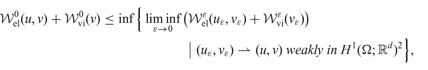
The above pointwise convergences are the classical heuristic linearization procedure. Still, one is left with actually checking that the finite-strain trajectories indeed converge to a solution of the linearized system. This is the aim of our second main result, Theorem 4.2, where we prove that, given a sequence of approximable solutions $(y_{\mathrm{vi},\epsilon },y_{\mathrm{el},\epsilon }{)}_{\epsilon }$ and upon defining $y_{\epsilon }=y_{\mathrm{el},\epsilon }°y_{\mathrm{vi},\epsilon }$ and the corresponding rescaled displacements $u_{\epsilon }=(y_{\epsilon }-\mathrm{i}{\mathrm{d}}_{\mathrm{\Omega }})/\epsilon$ and $v_{\epsilon }=(y_{\mathrm{vi},\epsilon }-\mathrm{i}{\mathrm{d}}_{\mathrm{\Omega }})/\epsilon$ , the sequence $(u_{\epsilon },v_{\epsilon }{)}_{\epsilon }$ converges pointwise in time (up to subsequences) to $(u,v):[0,T]\to H^1(\mathrm{\Omega };{\mathbb{R}}^d)\times H^1(\mathrm{\Omega };{\mathbb{R}}^d)$ with $(u(0),v(0))=(u^0,v^0):=\underset{\epsilon \to 0}{\lim }(u_{\epsilon }(0),v_{\epsilon }(0))$ and satisfying, for all $t\in [0,T]$ :

$\mathrm{Linearized}\mathrm{energy}\mathrm{in}\mathrm{equality}:$

$$\begin{array}{c}\frac{1}{2}{\int }_{\mathrm{\Omega }}\nabla (u(t)-v(t)):{\mathbb{C}}_{\mathrm{el}}\nabla (u(t)-v(t))\mathrm{d}X+\frac{1}{2}{\int }_{\mathrm{\Omega }}\nabla v(t):{\mathbb{C}}_{\mathrm{vi}}\nabla v(t)\mathrm{d}X-{\int }_{\mathrm{\Omega }}{f}^0(t)·u(t)\mathrm{d}X\hfill \\ +{\int }_0^t{\int }_{\mathrm{\Omega }}\mathbb{D}\nabla \stackrel{·}{v}(s):\nabla \stackrel{·}{v}(s)\mathrm{d}X\mathrm{d}s\hfill \\ \le \frac{1}{2}{\int }_{\mathrm{\Omega }}\nabla (u_0-v_0):{\mathbb{C}}_{\mathrm{el}}\nabla (u_0-v_0)\mathrm{d}X+\frac{1}{2}{\int }_{\mathrm{\Omega }}\nabla v_0:{\mathbb{C}}_{\mathrm{vi}}\nabla v_0\mathrm{d}X-{\int }_{\mathrm{\Omega }}{f}^0(0)·u_0\mathrm{d}X\hfill \\ -{\int }_0^t{\int }_{\mathrm{\Omega }}{\partial }_s{f}^0(s)·u(s)\mathrm{d}X\mathrm{d}s,\hfill \end{array}$$

(9)

$\mathrm{Linearized}\mathrm{semistability}:$

$$\begin{array}{c}\frac{1}{2}{\int }_{\mathrm{\Omega }}\nabla (u(t)-v(t)):{\mathbb{C}}_{\mathrm{el}}\nabla (u(t)-v(t))\mathrm{d}X-{\int }_{\mathrm{\Omega }}{f}^0(t)·u(t)\mathrm{d}X\hfill \\ \le \frac{1}{2}{\int }_{\mathrm{\Omega }}\nabla (\hat{u}-v(t)):{\mathbb{C}}_{\mathrm{el}}\nabla (\hat{u}-v(t))\mathrm{d}X-{\int }_{\mathrm{\Omega }}{f}^0(t)·\hat{u}\mathrm{d}X\forall \hat{u}\mathrm{admissible}.\hfill \end{array}$$

(10)

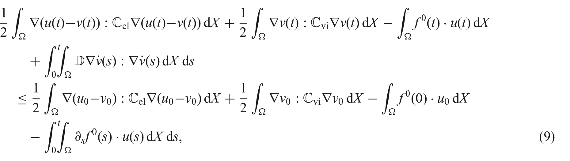
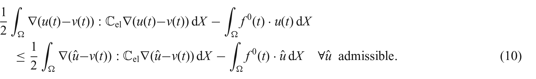
The linearized energy inequality and the linearized semistability deliver a weak notion of solution for the linearized problems (1) and (2). Albeit equations (9) and (10) are too weak to fully characterize the unique solution of linearized Poynting–Thomson systems (1) and (2), the equilibrium system (1) is fully recovered. In particular, $u$ is uniquely determined at all times, given $v$ . Moreover, the linearized energy equality (9) is sharp and turns out to be an equality in specific cases.

To conclude, let us note that one could alternatively perform the linearization at the time-discrete level and then pass to the time-continuous limit. This way one recovers the unique strong solution of the linearized Poynting–Thomson systems (1) and (2). This fact provides some additional justification of the finite-strain model. Still, we do not follow here this alternative path, which could be easily treated along the lines of the analysis in sections 6 and 7.

3. Preliminaries

We devote this section to setting notation and presenting some preliminary results.

3.1. Notation

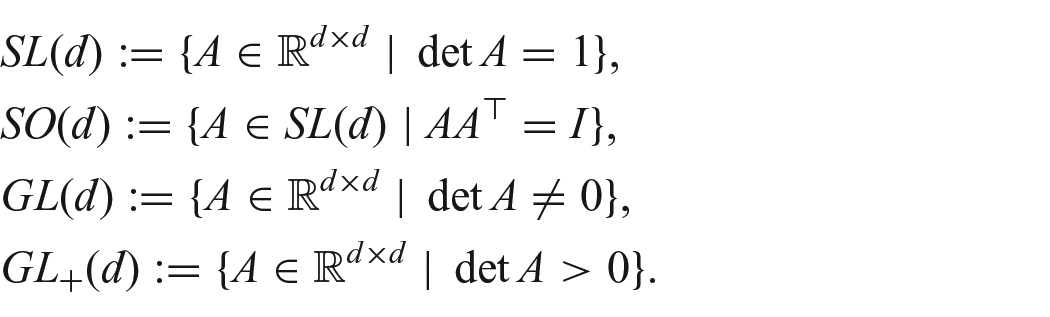
In what follows, we denote by ${\mathbb{R}}^{d\times d}$ the Euclidean space of $d\times d$ real matrices, $d\ge 2$ . Given $A\in {\mathbb{R}}^{d\times d}$ , we define its (Frobenius) norm as $|A{|}^2:=A:A$ , where the contraction product between two-tensors is defined as $A:B:=\sum _{i,j}{A}_{\mathrm{ij}}{B}_{\mathrm{ij}}$ . Moreover, given a symmetric positive definite four-tensor $\mathbb{C}\in {\mathbb{R}}^{d\times d\times d\times d}$ , the corresponding induced matrix norm is defined as $|A{|}_{\mathbb{C}}^2:=\mathbb{C}A:A/2$ . We denote by $A^{\mathrm{sym}}:=(A+A^{\top })/2$ the symmetric part of a matrix $A\in {\mathbb{R}}^{d\times d}$ . We will use the following matrix sets:

$$\begin{array}{c}\mathrm{SL}(d):=\{A\in {\mathbb{R}}^{d\times d}|detA=1\},\hfill \\ \mathrm{SO}(d):=\{A\in \mathrm{SL}(d)|A{A}^{\top }=I\},\hfill \\ \mathrm{GL}(d):=\{A\in {\mathbb{R}}^{d\times d}|detA\ne 0\},\hfill \\ G{L}_{+}(d):=\{A\in {\mathbb{R}}^{d\times d}|detA>0\}.\hfill \end{array}$$

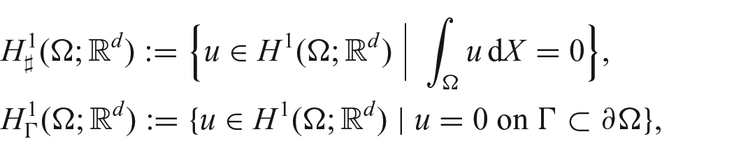
The symbol $B_r(A)\subset {\mathbb{R}}^{d\times d}$ denotes the open ball of radius $r>0$ and center $A\in {\mathbb{R}}^{d\times d}$ . We make use of the function spaces:

$$\begin{array}{c}{H}_{\#}^1(\mathrm{\Omega };{\mathbb{R}}^d):=\{u\in H^1(\mathrm{\Omega };{\mathbb{R}}^d)|{\int }_{\mathrm{\Omega }}u\mathrm{d}X=0\},\hfill \\ H_{\mathrm{\Gamma }}^1(\mathrm{\Omega };{\mathbb{R}}^d):=\{u\in H^1(\mathrm{\Omega };{\mathbb{R}}^d)|u=0\mathrm{on}\mathrm{\Gamma }\subset \partial \mathrm{\Omega }\},\hfill \end{array}$$

where $\mathrm{\Gamma }$ is a nonempty, open, and measurable subset of $\partial \mathrm{\Omega }$ .

Moreover, we denote by ${\mathcal{H}}^{d-1}$ the $(d-1)$ -dimensional Hausdorff measure and by $|\omega |$ the $d$ -dimensional Lebesgue measure of the measurable set $\omega$ in ${\mathbb{R}}^d$ .

3.2. Deformations and admissible states

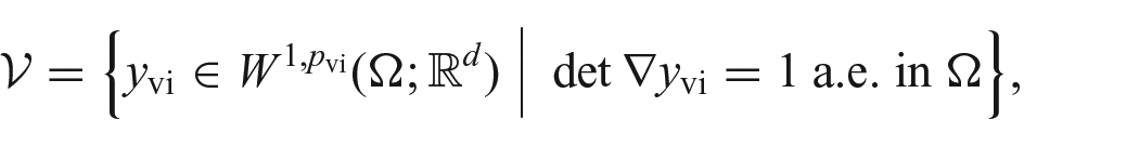
Let us fix the reference configuration $\mathrm{\Omega }$ of the body to be a nonempty, open, bounded, and connected Lipschitz subset of ${\mathbb{R}}^d$ . We assume without loss of generality that $\mathrm{\Omega }$ is such that ${\int }_{\mathrm{\Omega }}X\mathrm{d}X=0$ . We let ${\mathrm{\Gamma }}_D,{\mathrm{\Gamma }}_N$ be open subsets of $\partial \mathrm{\Omega }$ (in the relative topology of $\partial \mathrm{\Omega }$ ) such that ${\overline{\mathrm{\Gamma }}}_D\cup {\overline{\mathrm{\Gamma }}}_N=\partial \mathrm{\Omega }$ , ${\mathrm{\Gamma }}_D^{°}\cap {\mathrm{\Gamma }}_N^{°}=\varnothing$ , and ${\mathcal{H}}^{d-1}({\mathrm{\Gamma }}_D)>0$ .

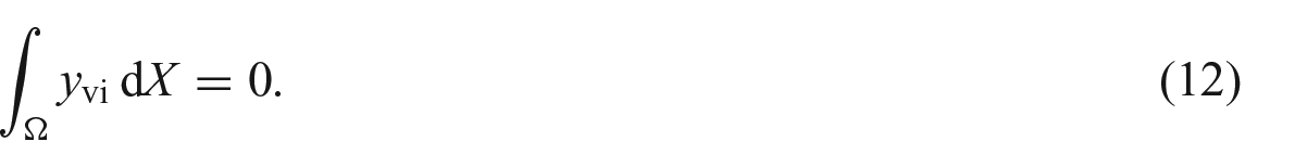
The viscous deformation is required to fulfill:

$$y_{\mathrm{vi}}\in W^{1,p_{\mathrm{vi}}}(\mathrm{\Omega };{\mathbb{R}}^d)\mathrm{for}\mathrm{some}{p}_{\mathrm{vi}}>d(d-1),$$

and to be locally volume-preserving, i.e., $det\nabla y_{\mathrm{vi}}=1$ almost everywhere in $\mathrm{\Omega }$ . In the following, $y_{\mathrm{vi}}$ is tacitly identified with its Hölder-continuous representative. More precisely, $y_{\mathrm{vi}}\in C^{0,1-d/p_{\mathrm{vi}}}(\mathrm{\Omega };{\mathbb{R}}^d)$ and is almost everywhere differentiable (see Fonseca and Gangbo [36]). In addition, since we will use the change-of-variables formula to pass from Lagrangian to Eulerian variables, we require $y_{\mathrm{vi}}$ to be injective almost everywhere. Equivalently, we ask for the Ciarlet–Nečas condition [37]:

$$|\mathrm{\Omega }|={\int }_{\mathrm{\Omega }}det\nabla y_{\mathrm{vi}}\mathrm{d}X=|y_{\mathrm{vi}}(\mathrm{\Omega })|,$$

(11)

to hold. As a consequence, we have the change-of-variables formula:

$${\int }_{\omega }\phi (y_{\mathrm{vi}}(X))\mathrm{d}X={\int }_{y_{\mathrm{vi}}(\omega )}\phi (\xi )\mathrm{d}\xi ,$$

for every measurable set $\omega \subseteq \mathrm{\Omega }$ and every measurable function $\phi :y_{\mathrm{vi}}(\omega )\to {\mathbb{R}}^d$ . Note that $y_{\mathrm{vi}}\in W^{1,p}(\mathrm{\Omega };{\mathbb{R}}^d)$ has distortion $K:=|\nabla y_{\mathrm{vi}}{|}^d/det\nabla y_{\mathrm{vi}}=|\nabla y_{\mathrm{vi}}{|}^d\in L^{p_{\mathrm{vi}}/d}(\mathrm{\Omega };\mathbb{R})$ , since it is locally volume preserving. As $p_{\mathrm{vi}}/d>d-1$ , this bound on the distortion $K$ implies that $y_{\mathrm{vi}}$ is either constant or open [38, Theorem 3.4]. By the Ciarlet–Nečas condition (11), $y_{\mathrm{vi}}$ cannot be constant, and hence, $y_{\mathrm{vi}}$ is open. In particular, $y_{\mathrm{vi}}(\mathrm{\Omega })$ is an open set. Moreover, we also have that $y_{\mathrm{vi}}$ is (globally) injective [39, Lemma 3.3] and that $y_{\mathrm{vi}}$ is actually a homeomorphism with inverse $y_{\mathrm{vi}}^{-1}\in W^{1,p_{\mathrm{vi}}/(d-1)}(y_{\mathrm{vi}}(\mathrm{\Omega });{\mathbb{R}}^d)$ (see Fonseca and Gangbo [36]).

In order to make the statement of the model precise, we need to require some regularity of the intermediate configuration $y_{\mathrm{vi}}(\mathrm{\Omega })$ . We recall the following definition.

Definition 3.1. ( $({\eta }_1,{\eta }_2)$ -Jones domain Jones [40]) Let ${\eta }_1,{\eta }_2>0$ . A bounded open set $\omega \subset {\mathbb{R}}^d$ is said to be a $({\eta }_1,{\eta }_2)$ -Jones domain, if for every $x,y\in \omega$ with $|x-y|<{\eta }_2$ there exists a Lipschitz curve $\gamma \in W^{1,\infty }([0,1];\omega )$ with $\gamma (0)=x$ and $\gamma (1)=y$ satisfying the following two conditions:

$$l(\gamma ):={\int }_0^1|\stackrel{·}{\gamma }(s)|\mathrm{d}s\le \frac{1}{{\eta }_1}|x-y|$$

and

$$d(\gamma (t),\partial \omega )\ge {\eta }_1\frac{|x-\gamma (t)||\gamma (t)-y|}{|x-y|}\mathrm{for}\mathrm{every}t\in [0,1].$$

The set of $({\eta }_1,{\eta }_2)$ -Jones domains will be denoted by ${\mathcal{J}}_{{\eta }_1,{\eta }_2}$ .

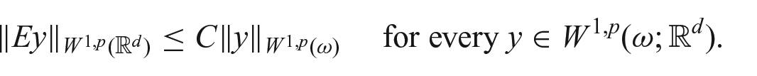
In the following, we will exploit the fact that $({\eta }_1,{\eta }_2)$ -Jones domains are Sobolev extension domains: for all ${\eta }_1,{\eta }_2>0$ , $p\in [1,\infty )$ , and all $\omega \in {\mathcal{J}}_{{\eta }_1,{\eta }_2}$ there exists a positive constant $C=C({\eta }_1,{\eta }_2,p,\omega ,d)$ and a linear operator $E:W^{1,p}(\omega ;{\mathbb{R}}^d)\to W^{1,p}({\mathbb{R}}^d;{\mathbb{R}}^d)$ such that $\mathrm{Ey}=y$ on $\omega$ and:

$$\parallel \mathrm{Ey}{\parallel }_{W^{1,p}({\mathbb{R}}^d)}\le C\parallel y{\parallel }_{W^{1,p}(\omega )}\mathrm{for}\mathrm{every}y\in W^{1,p}(\omega ;{\mathbb{R}}^d).$$

Note that the class of $({\eta }_1,{\eta }_2)$ -Jones domains is closed under Hausdorff convergence [13]. In the following, we will need to consider extensions and we then ask for the regularity:

$$y_{\mathrm{vi}}(\mathrm{\Omega })\in {\mathcal{J}}_{{\eta }_1,{\eta }_2}.$$

Finally, since the problem will be formulated only in terms of the gradient of $y_{\mathrm{vi}}$ , we impose the normalization condition:

$${\int }_{\mathrm{\Omega }}{y}_{\mathrm{vi}}\mathrm{d}X=0.$$

(12)

Given a viscous deformation $y_{\mathrm{vi}}$ , we assume the elastic deformation to fulfill:

$$y_{\mathrm{el}}\in W^{1,p_{\mathrm{el}}}(y_{\mathrm{vi}}(\mathrm{\Omega });{\mathbb{R}}^d)\mathrm{for}\mathrm{some}{p}_{\mathrm{el}}>d,$$

and we tacitly identify $y_{\mathrm{el}}$ with its Hölder-continuous representative.

For all given viscous deformation $y_{\mathrm{vi}}:\mathrm{\Omega }\to {\mathbb{R}}^d$ and elastic deformation $y_{\mathrm{el}}:y_{\mathrm{vi}}(\mathrm{\Omega }{)}^{°}\to {\mathbb{R}}^d$ , we define the total deformation as the composition of the two, i.e.,

$$y:=y_{\mathrm{el}}°y_{\mathrm{vi}}:\mathrm{\Omega }\to {\mathbb{R}}^d.$$

We assume that $y$ satisfies a Dirichlet boundary condition on ${\mathrm{\Gamma }}_D$ , namely:

$$y=\mathrm{id}\mathrm{on}{\mathrm{\Gamma }}_D.$$

(13)

Since $y_{\mathrm{vi}}$ is invertible and both $y_{\mathrm{vi}}$ and $y_{\mathrm{el}}$ are almost everywhere differentiable, the following chain rule:

$$\nabla y(X)=\nabla y_{\mathrm{el}}(y_{\mathrm{vi}}(X))\nabla y_{\mathrm{vi}}(X),$$

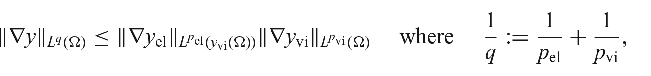
holds for almost every $X\in \mathrm{\Omega }$ . Hence, $y$ satisfies:

$$\parallel \nabla y{\parallel }_{L^q(\mathrm{\Omega })}\le \parallel \nabla y_{\mathrm{el}}{\parallel }_{L^{p_{\mathrm{el}}}(y_{\mathrm{vi}}(\mathrm{\Omega }))}\parallel \nabla y_{\mathrm{vi}}{\parallel }_{L^{p_{\mathrm{vi}}}(\mathrm{\Omega })}\mathrm{where}\frac{1}{q}:=\frac{1}{p_{\mathrm{el}}}+\frac{1}{p_{\mathrm{vi}}},$$

as can be readily checked by a change of variables and by the Hölder inequality. In particular, the boundary condition (13) should be understood in the classical trace sense.

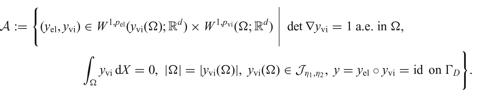
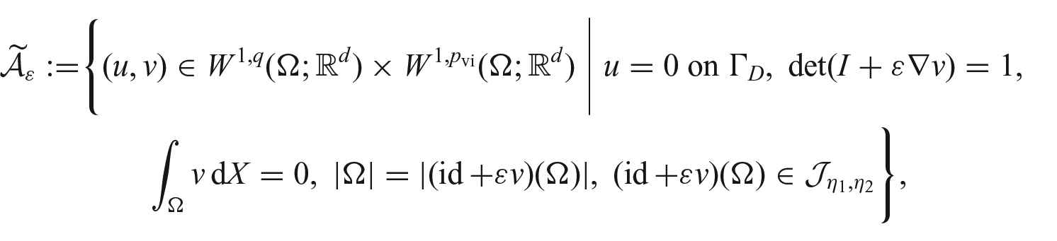
To sum up, the set of admissible states is defined as:

$$\begin{array}{c}\mathcal{A}:=\{(y_{\mathrm{el}},y_{\mathrm{vi}})\in W^{1,p_{\mathrm{el}}}(y_{\mathrm{vi}}(\mathrm{\Omega });{\mathbb{R}}^d)\times W^{1,p_{\mathrm{vi}}}(\mathrm{\Omega };{\mathbb{R}}^d)|det\nabla y_{\mathrm{vi}}=1\mathrm{a}.\mathrm{e}.\mathrm{in}\mathrm{\Omega },\hfill \\ {\int }_{\mathrm{\Omega }}{y}_{\mathrm{vi}}\mathrm{d}X=0,|\mathrm{\Omega }|=|y_{\mathrm{vi}}(\mathrm{\Omega })|,y_{\mathrm{vi}}(\mathrm{\Omega })\in {\mathcal{J}}_{{\eta }_1,{\eta }_2},y=y_{\mathrm{el}}°y_{\mathrm{vi}}=\mathrm{id}\mathrm{on}{\mathrm{\Gamma }}_D\}.\hfill \end{array}$$

Viscoelastic states are naturally depending on time. From now on, we are hence interested in trajectories $(y_{\mathrm{el}},y_{\mathrm{vi}}):[0,T]\to \mathcal{A}$ in the set of admissible states.

4. Main results

We devote this section to the statements of our assumptions and our main results.

4.1. Assumptions for the existence theory

In this section, we specify the assumptions needed for the existence results, namely, Proposition 4.1 and Theorem 4.1.

The total energy of the system at time $t\in [0,T]$ and state $(y_{\mathrm{el}},y_{\mathrm{vi}})\in \mathcal{A}$ is given by:

$$\mathcal{E}(t,y_{\mathrm{el}},y_{\mathrm{vi}}):=\mathcal{W}(y_{\mathrm{el}},y_{\mathrm{vi}})-〈\ell (t),y_{\mathrm{el}}°y_{\mathrm{vi}}〉,$$

where $\mathcal{W}(y_{\mathrm{el}},y_{\mathrm{vi}})$ is the stored energy and the pairing $〈\ell (t),y_{\mathrm{el}}°y_{\mathrm{vi}}〉$ represents the work of external mechanical actions.

More precisely, the stored energy is defined as:

$$\mathcal{W}(y_{\mathrm{el}},y_{\mathrm{vi}}):={\int }_{y_{\mathrm{vi}}(\mathrm{\Omega })}{W}_{\mathrm{el}}(\nabla y_{\mathrm{el}}(\xi ))\mathrm{d}\xi +{\int }_{\mathrm{\Omega }}{W}_{\mathrm{vi}}(\nabla y_{\mathrm{vi}}(X))\mathrm{d}X,$$

where $W_{\mathrm{el}}:{\mathbb{R}}^{d\times d}\to \mathbb{R}$ and $W_{\mathrm{vi}}:{\mathbb{R}}^{d\times d}\to \mathbb{R}\cup \{\infty \}$ are the stored elastic and the stored viscous energy densities, respectively. On the energy densities, we assume that:

(E1) there exist positive constants $c_1,c_2$ such that:

$$c_1|A{|}^{p_{\mathrm{el}}}\le W_{\mathrm{el}}(A)\le \frac{1}{c_1}(1+|A{|}^{p_{\mathrm{el}}})\mathrm{for}\mathrm{every}A\in \mathrm{GL}(d),$$

(14)

$$W_{\mathrm{vi}}(A)\ge \{\begin{array}{cc}{c}_2|A{|}^{p_{\mathrm{vi}}}-\frac{1}{c_2}\hfill & \mathrm{for}\mathrm{every}A\in \mathrm{SL}(d)\hfill \\ \multicolumn{1}{c}{\infty }& \mathrm{otherwise},\hfill \end{array}$$

(15)

for $p_{\mathrm{el}}>d$ and $p_{\mathrm{vi}}>d(d-1)$ .

(E2) $W_{\mathrm{el}},W_{\mathrm{vi}}$ are polyconvex, i.e., there exist two convex functions ${\hat{W}}_{\mathrm{el}},{\hat{W}}_{\mathrm{vi}}:{\mathbb{R}}^{\zeta (d)}\to \mathbb{R}\cup \{\infty \}$ such that:

$$W_{\mathrm{el}}(A)={\hat{W}}_{\mathrm{el}}(T(A))\mathrm{and}{W}_{\mathrm{vi}}(A)={\hat{W}}_{\mathrm{vi}}(T(A)),$$

where the minors $T(A)$ of $A$ are given by $T:{\mathbb{R}}^{d\times d}\to {\mathbb{R}}^{\zeta (d)}$ :

$$T(A):=(A,\mathrm{ad}{\mathrm{j}}_{2}A,\cdots ,\mathrm{ad}{\mathrm{j}}_{d}A),$$

here, ${\mathrm{adj}}_{s}A$ denotes the matrix of all minors $s\times s$ of the matrix $A\in {\mathbb{R}}^{d\times d}$ , for $s=2,\cdots ,d$ and $\zeta (d):=\sum _{s=1}^d{\left(\begin{array}{c}s\hfill \\ \multicolumn{1}{c}{d}\end{array}\right)}^2$ .

Notice that, since $p_{\mathrm{vi}}>d$ , the mapping $y_{\mathrm{vi}}\to \mathrm{ad}{\mathrm{j}}_s\nabla y_{\mathrm{vi}}$ is $(W^{1,p_{\mathrm{vi}}},L^{p_{\mathrm{vi}}/s})$ -weakly sequentially continuous. Hence, given $y_{\mathrm{vi},n}\rightharpoonup y_{\mathrm{vi}}$ in $W^{1,p_{\mathrm{vi}}}(\mathrm{\Omega };{\mathbb{R}}^d)$ with $det\nabla y_{\mathrm{vi},n}=1$ almost everywhere in $\mathrm{\Omega }$ , we have that:

$$1=det\nabla y_{\mathrm{vi},n}\rightharpoonup det\nabla y_{\mathrm{vi}}=1\mathrm{in}{L}^{p_{\mathrm{vi}}/d}(\mathrm{\Omega }).$$

As $\nabla y_{\mathrm{vi}}(X)\in \mathrm{SL}(d)$ a.e. in $\mathrm{\Omega }$ , we have that:

$${\int }_{\mathrm{\Omega }}{W}_{\mathrm{vi}}(\nabla y_{\mathrm{vi}}(X))\mathrm{d}X\le \underset{n}{\lim \inf }{\int }_{\mathrm{\Omega }}{W}_{\mathrm{vi}}(\nabla y_{\mathrm{vi},n}(X))\mathrm{d}X,$$

by polyconvexity of $W_{\mathrm{vi}}$ . In particular, $y_{\mathrm{vi}}\to {\int }_{\mathrm{\Omega }}{W}_{\mathrm{vi}}(\nabla y_{\mathrm{vi}}(X))\mathrm{dX}$ is weakly lower semicontinuous in $W^{1,p_{\mathrm{vi}}}(\mathrm{\Omega };{\mathbb{R}}^d)$ .

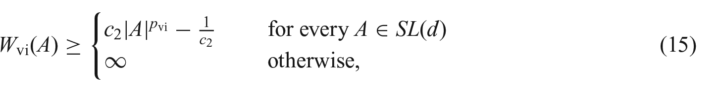
The growth condition (15) ensures that all viscous deformations $y_{\mathrm{vi}}$ of finite energy are incompressible. Local elastic incompressibility $det\nabla y_{\mathrm{el}}=1$ or even the weaker $det\nabla y_{\mathrm{el}}>0$ cannot be required, however. This is due to the fact that we later need to consider the Sobolev extension of $y_{\mathrm{el}}$ from the moving domain $y_{\mathrm{vi}}(\mathrm{\Omega })$ to ${\mathbb{R}}^d$ in order to compute the limit of an infimizing sequence. As it is well-known, such extensions may not preserve the positivity of $det\nabla y_{\mathrm{el}}$ .

On the contrary, our assumptions on the elastic energy density are compatible with frame indifference. In particular, we could ask $W_{\mathrm{el}}(\mathrm{RA})=W_{\mathrm{el}}(A)$ for every rotation $R\in \mathrm{SO}(d)$ and every $A\in {\mathbb{R}}^{d\times d}$ . Note nonetheless that this property, although fundamental from the mechanical standpoint, is actually not needed for the analysis. The above assumptions would be compatible with requiring that $W_{\mathrm{vi}}$ is invariant by left multiplication with special rotations, as well. Still, such an invariance would be little relevant from the modeling viewpoint, for the viscous energy density is defined on viscous deformations, which take values in the intermediate configuration.

Eventually, the work of external mechanical actions is assumed to result from a given time-dependent body force $f:[0,T]\times \mathrm{\Omega }\to {\mathbb{R}}^d$ and a given time-dependent boundary traction $g:[0,T]\times {\mathrm{\Gamma }}_N\to {\mathbb{R}}^d$ as follows:

$$〈\ell (t),y〉:={\int }_{\mathrm{\Omega }}f(t,X)·y(X)\mathrm{d}X+{\int }_{{\mathrm{\Gamma }}_N}g(t,X)·y(X)\mathrm{d}{\mathcal{H}}^{d-1}(X).$$

(16)

We assume:

(E3) $f\in W^{1,\infty }(0,T;L^{(q^{*}{)}^{\prime }}(\mathrm{\Omega };{\mathbb{R}}^d))$ and $g\in W^{1,\infty }(0,T;L^{(q^{\#}{)}^{\prime }}({\mathrm{\Gamma }}_N;{\mathbb{R}}^d))$ where $q^{*}$ and $q^{\#}$ are the Sobolev and trace exponent related to $W^{1,q}(\mathrm{\Omega };{\mathbb{R}}^d)$ , respectively (see Roubíček [41]) and the prime denotes conjugation.

Consequently, we have:

$$\ell \in W^{1,\infty }(0,T;(W^{1,q}(\mathrm{\Omega };{\mathbb{R}}^d{))}^{*}),$$

where $(W^{1,q}(\mathrm{\Omega };{\mathbb{R}}^d){)}^{*}$ is the dual space of $W^{1,q}(\mathrm{\Omega };{\mathbb{R}}^d)$ .

Given a time-dependent viscous trajectory $y_{\mathrm{vi}}:[0,T]\to W^{1,p_{\mathrm{vi}}}(\mathrm{\Omega };{\mathbb{R}}^d)$ , we define the total instantaneous dissipation of the system [11] as:

$$\mathrm{\Psi }(y_{\mathrm{vi}},{\stackrel{·}{y}}_{\mathrm{vi}}):={\int }_{\mathrm{\Omega }}\psi (\nabla {\stackrel{·}{y}}_{\mathrm{vi}}(\nabla y_{\mathrm{vi}}{)}^{-1})\mathrm{d}X.$$

(17)

Here and in the following, the dot represents a partial derivative with respect to time. Above, the dissipation density $\psi :{\mathbb{R}}^{d\times d}\to [0,\infty )$ is assumed to be:

(E4) convex and differentiable at $0$ with $\psi (0)=0$ ;

(E5) fulfilling:

$$\psi (A)\ge c_3|A{|}^{p_{\psi }}\mathrm{for}\mathrm{every}A\in {\mathbb{R}}^{d\times d},$$

(18)

for some positive constant $c_3$ ;

(E6) positively $p_{\psi }$ -homogeneous, namely:

$$\psi (\lambda A)={\lambda }^{p_{\psi }}\psi (A)\mathrm{for}\mathrm{every}A\in {\mathbb{R}}^{d\times d},\lambda \ge 0.$$

(19)

The form of the instantaneous dissipation is parallel to the analogous definition in elastoplasticity, where nonetheless $\psi$ is assumed to be positively $1$ -homogeneous, namely, $p_{\psi }=1$ [42, 43]. In particular, let us explicitly point out that it does not fall within the frame-indifferent setting from Antman [44]. Indeed, in this case, viscous deformations take values in the intermediate configuration only and frame-indifference should not necessarily be imposed there.

In the following, we ask:

$$p_{\psi }\ge 2\ge \frac{d(d-1)}{d(d-1)-1},$$

(20)

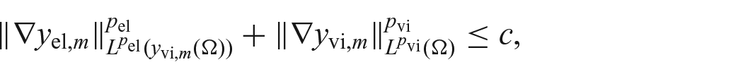
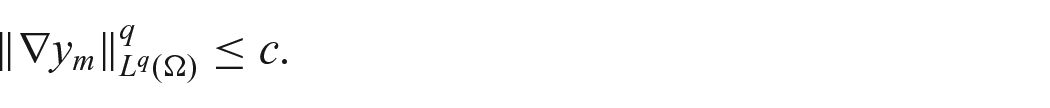
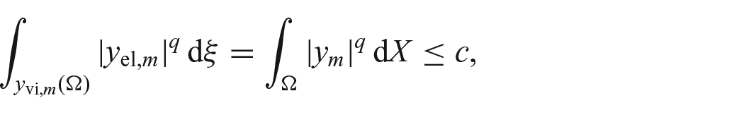
where we have used $d\ge 2$ . In particular, we have that $p_{\psi }^{\prime }<p_{\psi }$ and, by defining $p_r$ by $1/p_r:=1/p_{\psi }+1/p_{\mathrm{vi}}$ , one has that $p_r>1$ . Again by Hölder’s inequality, this entails that:

$$\parallel \nabla {\stackrel{·}{y}}_{\mathrm{vi}}{\parallel }_{L^{p_r}(\mathrm{\Omega })}\le \parallel \nabla {\stackrel{·}{y}}_{\mathrm{vi}}(\nabla y_{\mathrm{vi}}{)}^{-1}{\parallel }_{L^{p_{\psi }}(\mathrm{\Omega })}\parallel \nabla y_{\mathrm{vi}}{\parallel }_{L^{p_{\mathrm{vi}}}(\mathrm{\Omega })}\le c\mathrm{\Psi }(y_{\mathrm{vi}},{\stackrel{·}{y}}_{\mathrm{vi}})(\mathcal{W}{(y_{\mathrm{el}},y_{\mathrm{vi}})}^{1/p_{\mathrm{vi}}}+1).$$

In particular, $\nabla {\stackrel{·}{y}}_{\mathrm{vi}}$ belongs to $L^{p_r}(\mathrm{\Omega };{\mathbb{R}}^{d\times d})$ with $p_r>1$ whenever energy and dissipation are finite.

Here and in the following, the symbol $c$ denotes a generic positive constant, possibly depending on data and changing from line to line.

4.2. Existence results

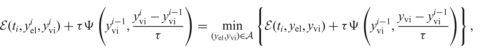
Before presenting the statements of our main results, we make the notion of solution to the problem precise. To this aim, let ${\mathrm{\Pi }}_{\tau }:=\{0=t_0<t_1<...<t_N=T\}$ denote the uniform partition of the time interval $[0,T]$ with time step $t_i-t_{i-1}=\tau >0$ for every $i=1,\dots ,N_{:}=T/\tau$ . From now on, let $(y_{\mathrm{el},0},y_{\mathrm{vi},0})$ be a compatible initial condition, i.e.,

$$(y_{\mathrm{el},0},y_{\mathrm{vi},0})\in \mathcal{A}\mathrm{with}\mathcal{E}(0,y_{\mathrm{el},0},y_{\mathrm{vi},0})<\infty .$$

(21)

Given $(y_{\mathrm{el}}^0,y_{\mathrm{vi}}^0):=(y_{\mathrm{el},0},y_{\mathrm{vi},0})$ , for all $i=1,...,N$ , we define the incremental minimization problems:

$$\underset{(y_{\mathrm{el}},y_{\mathrm{vi}})\in \mathcal{A}}{min}\{\mathcal{E}(t_i,y_{\mathrm{el}},y_{\mathrm{vi}})+\tau \mathrm{\Psi }(y_{\mathrm{vi}}^{i-1},\frac{y_{\mathrm{vi}}-y_{\mathrm{vi}}^{i-1}}{\tau })\}.$$

(22)

We call a sequence of minimizers $(y_{\mathrm{el}}^i,y_{\mathrm{vi}}^i{)}_{i=0}^N$ of equation (22) an incremental solution of the problem corresponding to time step $\tau$ .

Note that incremental solutions exist. In particular, we have the following.

Proposition 4.1. (Existence of incremental solutions) Under assumptions (E1)– (E5) of section 4.1 and equation (21), the incremental minimization problem (22) admits an incremental solution $(y_{\mathrm{el}}^i,y_{\mathrm{vi}}^i{)}_{i=0}^N\subset \mathcal{A}$ .

The proof of Proposition 4.1 is given in section 5.

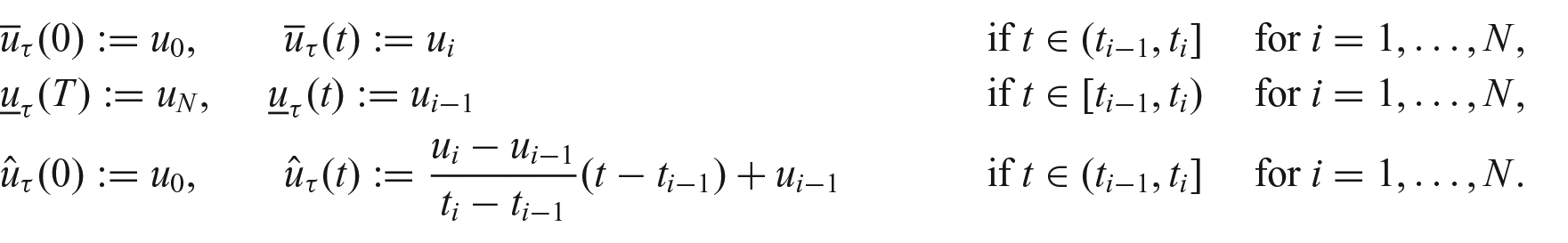
In the following, we make use of the following notation for interpolations. Given a vector $(u_0,...,u_N)$ , we define its backward-constant interpolant ${\overline{u}}_{\tau }$ , its forward-constant interpolant ${\underset{¯}{u}}_{\tau }$ , and its piecewise-affine interpolant ${\hat{u}}_{\tau }$ on the partition ${\mathrm{\Pi }}_{\tau }$ as:

$$\begin{array}{c}{\overline{u}}_{\tau }(0):=u_0,{\overline{u}}_{\tau }(t):=u_i\mathrm{if}t\in (t_{i-1},t_i]\mathrm{for}i=1,\dots ,N,\hfill \\ {\underset{¯}{u}}_{\tau }(T):=u_N,{\underset{¯}{u}}_{\tau }(t):=u_{i-1}\mathrm{if}t\in [t_{i-1},t_i)\mathrm{for}i=1,\dots ,N,\hfill \\ {\hat{u}}_{\tau }(0):=u_0,{\hat{u}}_{\tau }(t):=\frac{u_i-u_{i-1}}{t_i-t_{i-1}}(t-t_{i-1})+u_{i-1}\mathrm{if}t\in (t_{i-1},t_i]\mathrm{for}i=1,\dots ,N.\hfill \end{array}$$

We are now in the position of introducing our notion of solution to the large-strain Poynting–Thomson model.

Definition 4.1. (Approximable solution) We call $(y_{\mathrm{el}},y_{\mathrm{vi}}):[0,T]\to \mathcal{A}$ an approximable solution if there exists a sequence of uniform partitions of the interval $[0,T]$ with mesh size $\tau \to 0$ , corresponding incremental solutions $(y_{\mathrm{el}}^i,y_{\mathrm{vi}}^i{)}_{i=0}^N$ , and a nondecreasing function $\delta :[0,T]\to [0,\infty )$ such that, for every $0\le s\le t\le T$ ,

$\mathrm{Approximation}:$

$$\begin{array}{c}({\overline{y}}_{\mathrm{el},\tau }(t),{\overline{y}}_{\mathrm{vi},\tau }(t))\rightharpoonup (y_{\mathrm{el}}(t),y_{\mathrm{vi}}(t))\mathrm{in}{W}_{\mathrm{loc}}^{1,p_{\mathrm{el}}}(y_{\mathrm{vi}}(t,\mathrm{\Omega });{\mathbb{R}}^d)\times W^{1,p_{\mathrm{vi}}}(\mathrm{\Omega };{\mathbb{R}}^d),\hfill \\ {\int }_0^t\mathrm{\Psi }({\underset{¯}{y}}_{\mathrm{vi},\tau },{\stackrel{·}{\hat{y}}}_{\mathrm{vi},\tau })\to \delta (t),\hfill \\ {\int }_s^t\mathrm{\Psi }({\underset{¯}{y}}_{\mathrm{vi},\tau },{\stackrel{·}{\hat{y}}}_{\mathrm{vi},\tau })\le \delta (t)-\delta (s),\hfill \end{array}$$

$\mathrm{Energy}\mathrm{inequality}:$

$$\mathcal{E}(t,y_{\mathrm{el}},y_{\mathrm{vi}})+p_{\psi }\delta (t)\le \mathcal{E}(0,y_{\mathrm{el},0},y_{\mathrm{vi},0})-{\int }_0^t〈\stackrel{·}{\ell }(s),y〉,$$

(23)

$\mathrm{Semistability}:$

$$\mathcal{E}(t,y_{\mathrm{el}}(t),y_{\mathrm{vi}}(t))\le \mathcal{E}(t,{\tilde{y}}_{\mathrm{el}},y_{\mathrm{vi}}(t))\forall {\tilde{y}}_{\mathrm{el}}\mathrm{with}({\tilde{y}}_{\mathrm{el}},y_{\mathrm{vi}}(t))\in \mathcal{A}.$$

(24)

Our first main result concerns the existence of approximable solutions.

Theorem 4.1. (Existence of approximable solutions) Under the assumptions (E1)–(E6) of section 4.1 and equation (21), there exists an approximable solution $(y_{\mathrm{el}},y_{\mathrm{vi}}):[0,T]\to \mathcal{A}$ .

The proof of Theorem 4.1 is detailed in section 6.

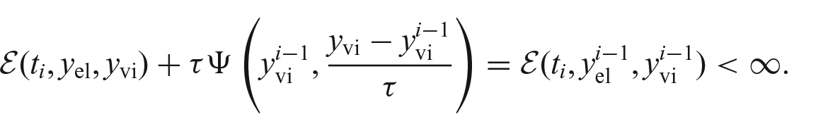
As already mentioned in the introduction, the fact that solutions are approximable ensures that viscous evolution actually occurs, even in the absence of applied loads. We show this fact by resorting to the simplest, scalar model at a single material point. We consider the energy densities, the dissipation to be quadratic, and that no loading is present. More precisely, we let $F\in \mathbb{R}$ and $F_{\mathrm{vi}}>0$ represent the total and viscous (scalar) strains, respectively, we define $W_{\mathrm{el}}(F_{\mathrm{el}})=W_{\mathrm{el}}({\mathrm{FF}}_{\mathrm{vi}}^{-1}):=\frac{1}{2}|{\mathrm{FF}}_{\mathrm{vi}}^{-1}-1{|}^2$ , $W_{\mathrm{vi}}(F_{\mathrm{vi}}):=\frac{1}{2}|F_{\mathrm{vi}}-1{|}^2$ , $\psi ({\stackrel{·}{F}}_{\mathrm{vi}}{F}_{\mathrm{vi}}^{-1}):=\frac{1}{2}|{\stackrel{·}{F}}_{\mathrm{vi}}{F}_{\mathrm{vi}}^{-1}{|}^2$ , and we let $\ell (t)\equiv 0$ for every $t\in [0,T]$ . In this setting, the discrete incremental problem (22) is specified as:

$$\underset{F\in \mathbb{R},F_{\mathrm{vi}}>0}{min}(\frac{1}{2}{|{\mathrm{FF}}_{\mathrm{vi}}^{-1}-1|}^2+\frac{1}{2}|F_{\mathrm{vi}}-{1|}^2+\frac{1}{2\tau }{|(F_{\mathrm{vi}}-F_{\mathrm{vi}}^{i-1})(F_{\mathrm{vi}}^{i-1}{)}^{-1}|}^2)\mathrm{for}i=1,\dots ,N.$$

(25)

Take now initial values $(F^0,F_{\mathrm{vi}}^0)$ with $F_{\mathrm{vi}}^0\ne 1$ , so that some nonvanishing viscous stress present at time $0$ . In this case, it is easy to check that the constant in time solution $(F^0,F_{\mathrm{vi}}^0)$ satisfies the energy inequality and semistability, but it is not approximable. This implies that the viscous strain $F_{\mathrm{vi}}$ corresponding to an approximable solution must evolve with time (see Figure 2). In this simple setting, asking the solution of the continuous problem to be approximable indeed implies uniqueness, as all discrete trajectories converge to the unique solution of the limiting differential problem.

4.3. Assumptions for the linearization theory

In addition to the assumptions stated in section 4.1, we will require the following conditions in order to prove the linearization result.

On the stored elastic energy density $W_{\mathrm{el}}$ , we assume that:

(L1) $W_{\mathrm{el}}$ is locally Lipschitz;

(L2) $W_{\mathrm{el}}$ satisfies the growth condition:

$$W_{\mathrm{el}}(A)\ge c_4\mathrm{dis}{\mathrm{t}}^2(A,\mathrm{SO}(d)),$$

(26)

for some $c_4>0$ ;

(L3) there exists a positive definite tensor ${\mathbb{C}}_{\mathrm{el}}$ such that, for every $\delta >0$ , there exists $c_{\mathrm{el}}(\delta )>0$ satisfying:

$$|W_{\mathrm{el}}(I+A)-|A{|}_{{\mathbb{C}}_{\mathrm{el}}}^2|\le \delta |A{|}_{{\mathbb{C}}_{\mathrm{el}}}^2\mathrm{for}\mathrm{every}A\in B_{c_{\mathrm{el}}(\delta )}(0).$$

(27)

In particular, these conditions imply that ${\mathbb{C}}_{\mathrm{el}}$ is symmetric and:

$$c_4|A^{\mathrm{sym}}{|}^2\le |A{|}_{{\mathbb{C}}_{\mathrm{el}}}^2\mathrm{for}\mathrm{every}A\in {\mathbb{R}}^{d\times d}.$$

We can also equivalently state inequality (27) as follows:

$$(1-\delta )|A{|}_{{\mathbb{C}}_{\mathrm{el}}}^2\le W_{\mathrm{el}}(I+A)\le (1+\delta )|A{|}_{{\mathbb{C}}_{\mathrm{el}}}^2\mathrm{for}\mathrm{every}A\in B_{c_{\mathrm{el}}(\delta )}(0).$$

(28)

Concerning the viscous stored energy density $W_{\mathrm{vi}}$ , we ask that:

(L4)

$$W_{\mathrm{vi}}(A)=\{\begin{array}{cc}{\tilde{W}}_{\mathrm{vi}}(A)\hfill & \mathrm{if}A\in K\hfill \\ \multicolumn{1}{c}{\infty }& \mathrm{otherwise},\hfill \end{array}$$

where $K\subset \subset \mathrm{SL}(d)$ contains a neighborhood of the identity;

(L5) ${\tilde{W}}_{\mathrm{vi}}$ is locally Lipschitz continuous in a neighborhood of the identity and:

$${\tilde{W}}_{\mathrm{vi}}(I+A)\ge c_5|A{|}^2\mathrm{for}\mathrm{every}A\in {\mathbb{R}}^{d\times d}\mathrm{with}I+A\in K,$$

(29)

for some $c_5>0$ ;

(L6) there exists a positive definite tensor ${\mathbb{C}}_{\mathrm{vi}}$ such that, for every $\delta >0$ , there exists $c_{\mathrm{vi}}(\delta )>0$ satisfying:

$$|{\tilde{W}}_{\mathrm{vi}}(I+A)-|A{|}_{{\mathbb{C}}_{\mathrm{vi}}}^2|\le \delta |A{|}_{{\mathbb{C}}_{\mathrm{vi}}}^2\mathrm{for}\mathrm{every}A\in B_{c_{\mathrm{vi}}(\delta )}(0),$$

or, equivalently,

$$(1-\delta )|A{|}_{{\mathbb{C}}_{\mathrm{vi}}}^2\le {\tilde{W}}_{\mathrm{vi}}(I+A)\le (1+\delta )|A{|}_{{\mathbb{C}}_{\mathrm{vi}}}^2\mathrm{for}\mathrm{every}A\in B_{c_{\mathrm{vi}}(\delta )}(0).$$

(30)

As above, we have that:

$$c_5|A^{\mathrm{sym}}{|}^2\le |A{|}_{{\mathbb{C}}_{\mathrm{vi}}}^2\mathrm{for}\mathrm{every}A\in {\mathbb{R}}^{d\times d}.$$

Moreover, there exists a constant $c_K>0$ (depending only on the compact set $K$ ) such that:

$$|A|+|A^{-1}|\le c_K\mathrm{for}\mathrm{every}A\in K$$

(31)

and

$$|A-I|\ge \frac{1}{c_K}\mathrm{for}\mathrm{every}A\in \mathrm{SL}(d)\backslash K.$$

These last two inequalities will provide $L^{\infty }$ -bounds on the terms $\epsilon \nabla v$ and $(I+\epsilon \nabla v{)}^{-1}$ later on. Note, however, that the effect of the constraint $K$ will disappear as $\epsilon \to 0$ . In particular, the limiting linearized problem is independent of $K$ .

On the forcing term ${\ell }^0$ , we assume that:

(L7) ${\ell }^0\in W^{1,1}(0,T;(H^1(\mathrm{\Omega };{\mathbb{R}}^d{))}^{*})$ .

Finally, on the dissipation density $\psi$ , we assume that:

(L8) $\psi$ satisfies the growth condition:

$$\psi (A)\ge c_6|A{|}^2\mathrm{for}\mathrm{every}A\in {\mathbb{R}}^{d\times d},$$

(32)

for some $c_6>0$ ;

(L9) there exists a positive definite tensor $\mathbb{D}$ such that, for every $\delta >0$ , there exists $c_{\psi }(\delta )>0$ satisfying:

$$|\psi (A)-|A{|}_{\mathbb{D}}^2|\le \delta |A{|}_{\mathbb{D}}^2\mathrm{for}\mathrm{every}A\in B_{c_{\psi }(\delta )}(0);$$

(33)

(L10) $\psi$ is positively two-homogeneous, i.e.,

$$\psi (\lambda A)={\lambda }^2\psi (A)\mathrm{for}\mathrm{every}A\in {\mathbb{R}}^{d\times d},\lambda \ge 0.$$

The specification $p_{\psi }=2$ of assumption (L10) (compare with the more general $p_{\psi }\ge 2$ from (E6)) is just needed in the linearization setting to recover the linearized energy inequality (37).

4.4. Linearization result

Before moving on, let us reformulate the setting and the existence results of Proposition 4.1 and Theorem 4.1 in terms of the linearization variables $u$ and $v$ . For all $\epsilon >0$ fixed, the admissible set $\mathcal{A}$ is equivalently rewritten as:

$$\begin{array}{c}{\tilde{\mathcal{A}}}_{\epsilon }:=\{(u,v)\in W^{1,q}(\mathrm{\Omega };{\mathbb{R}}^d)\times W^{1,p_{\mathrm{vi}}}(\mathrm{\Omega };{\mathbb{R}}^d)|u=0\mathrm{on}{\mathrm{\Gamma }}_D,det(I+\epsilon \nabla v)=1,\hfill \\ \multicolumn{1}{c}{{\int }_{\mathrm{\Omega }}v\mathrm{d}X=0,|\mathrm{\Omega }|=|(\mathrm{id}+\epsilon v)(\mathrm{\Omega })|,(\mathrm{id}+\epsilon v)(\mathrm{\Omega })\in {\mathcal{J}}_{{\eta }_1,{\eta }_2}\},}\end{array}$$

where we recall that $\mathrm{\Omega }$ is chosen to be such that: ${\int }_{\mathrm{\Omega }}\mathrm{X}\mathrm{d}X=0$ so that:

$$0\stackrel{(12)}{=}{\int }_{\mathrm{\Omega }}{y}_{\mathrm{vi}}\mathrm{d}X={\int }_{\mathrm{\Omega }}(\mathrm{id}+\epsilon v)\mathrm{d}X=\epsilon {\int }_{\mathrm{\Omega }}v\mathrm{d}X.$$

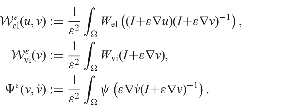
We use the following notation for the rescaled energies and dissipation:

$$\begin{array}{c}{\mathcal{W}}_{\mathrm{el}}^{\epsilon }(u,v):=\frac{1}{{\epsilon }^2}{\int }_{\mathrm{\Omega }}{W}_{\mathrm{el}}((I+\epsilon \nabla u)(I+\epsilon \nabla v{)}^{-1}),\hfill \\ {\mathcal{W}}_{\mathrm{vi}}^{\epsilon }(v):=\frac{1}{{\epsilon }^2}{\int }_{\mathrm{\Omega }}{W}_{\mathrm{vi}}(I+\epsilon \nabla v),\hfill \\ {\mathrm{\Psi }}^{\epsilon }(v,\stackrel{·}{v}):=\frac{1}{{\epsilon }^2}{\int }_{\mathrm{\Omega }}\psi (\epsilon \nabla \stackrel{·}{v}{(I+\epsilon \nabla v)}^{-1}).\hfill \end{array}$$

Their corresponding linearized counterparts read:

$$\begin{array}{c}{\mathcal{W}}_{\mathrm{el}}^0(u,v):=\frac{1}{2}{\int }_{\mathrm{\Omega }}\nabla (u-v):{\mathbb{C}}_{\mathrm{el}}\nabla (u-v),\hfill \\ {\mathcal{W}}_{\mathrm{vi}}^0(v):=\frac{1}{2}{\int }_{\mathrm{\Omega }}\nabla v:{\mathbb{C}}_{\mathrm{vi}}\nabla v,\hfill \\ {\mathrm{\Psi }}^0(\stackrel{·}{v}):=\frac{1}{2}{\int }_{\mathrm{\Omega }}\mathbb{D}\nabla \stackrel{·}{v}:\nabla \stackrel{·}{v}.\hfill \end{array}$$

We also define for brevity:

$${\mathcal{E}}^{\epsilon }(u,v):={\mathcal{W}}_{\mathrm{vi}}^{\epsilon }(v)+{\mathcal{W}}_{\mathrm{el}}^{\epsilon }(u,v)-〈{\ell }^0,u〉\mathrm{and}{\mathcal{E}}^0(u,v):={\mathcal{W}}_{\mathrm{vi}}^0(v)+{\mathcal{W}}_{\mathrm{el}}^0(u,v)-〈{\ell }^0,u〉.$$

Finally, let $(u_{\epsilon }^0,v_{\epsilon }^0)\in {\tilde{\mathcal{A}}}_{\epsilon }$ be a well-prepared sequence of initial data, namely:

$$(u_{\epsilon }^0,v_{\epsilon }^0)\rightharpoonup (u^0,v^0)\mathrm{in}{H}^1(\mathrm{\Omega })\times H^1(\mathrm{\Omega })\mathrm{and}\underset{\epsilon \to 0}{\lim }{\mathcal{E}}^{\epsilon }(u_{\epsilon }^0,v_{\epsilon }^0)={\mathcal{E}}^0(u^0,v^0).$$

(34)

Proposition 4.1 and Theorem 4.1 can therefore be rewritten in terms of the new variables $(u,v)$ and in the presence of the rescaling prefactor $1/{\epsilon }^2$ as follows.

Corollary 4.1. (Existence in terms of $(u_{\epsilon },v_{\epsilon })$ ) Under the assumptions (E1)–(E5) and (L10) of section 4.1 and equation (34) for every $\epsilon >0$ , there exists a sequence of partitions $({\mathrm{\Pi }}_{{\tau }^{\epsilon }}{)}_{{\tau }^{\epsilon }}$ of the interval $[0,T]$ with mesh size ${\tau }^{\epsilon }\to 0$ and functions $(u_{\epsilon },v_{\epsilon }):[0,T]\to {\tilde{\mathcal{A}}}_{\epsilon }$ such that for every $t\in [0,T]$ :

$\mathrm{Approximation}:$

$$({\overline{u}}_{{\tau }^{\epsilon }}(t),{\overline{v}}_{{\tau }^{\epsilon }}(t))\rightharpoonup (u_{\epsilon }(t),v_{\epsilon }(t))\mathrm{in}{W}^{1,q}(\mathrm{\Omega };{\mathbb{R}}^d)\times W^{1,p_{\mathrm{vi}}}(\mathrm{\Omega };{\mathbb{R}}^d).$$

$\mathrm{Energy}\mathrm{inequality}:$

$$\begin{array}{c}{\mathcal{W}}_{\mathrm{vi}}^{\epsilon }(v_{\epsilon }(t))+{\mathcal{W}}_{\mathrm{el}}^{\epsilon }(u_{\epsilon }(t),v_{\epsilon }(t))-〈{\ell }^0,u_{\epsilon }(t)〉+2{\int }_0^t{\mathrm{\Psi }}^{\epsilon }(v_{\epsilon },{\stackrel{·}{v}}_{\epsilon })\hfill \\ \le {\mathcal{W}}_{\mathrm{vi}}^{\epsilon }(v_{\epsilon }^0)+{\mathcal{W}}_{\mathrm{el}}^{\epsilon }(u_{\epsilon }^0,v_{\epsilon }^0)-{\int }_0^t〈{\stackrel{·}{\ell }}^0,u_{\epsilon }〉.\hfill \end{array}$$

(35)

$\mathrm{Semistability}:$

$$\begin{array}{c}{\mathcal{W}}_{\mathrm{el}}^{\epsilon }(u_{\epsilon }(t),v_{\epsilon }(t))-〈{\ell }^{\epsilon }(t),u_{\epsilon }(t)〉\le {\mathcal{W}}_{\mathrm{el}}^{\epsilon }({\tilde{u}}_{\epsilon },v_{\epsilon }(t))-〈{\ell }^{\epsilon }(t),{\tilde{u}}_{\epsilon }(t)〉\hfill \\ \forall {\tilde{u}}_{\epsilon }\mathrm{with}({\tilde{u}}_{\epsilon },v_{\epsilon }(t))\in {\tilde{\mathcal{A}}}_{\epsilon }.\hfill \end{array}$$

(36)

In the following result, we show that a sequence $(u_{\epsilon },v_{\epsilon }{)}_{\epsilon }$ of approximable solutions at level $\epsilon$ converges weakly to $(u,v)$ satisfying the linearized energy and the linearized semistability inequalities.

Theorem 4.2. (Linearization) For every $\epsilon >0$ ,let $(u_{\epsilon },v_{\epsilon })$ be an approximable solutions given as in Corollary 4.1. Then, under the assumptions (L1)–(L10) of section 4.3 and equation (34), there exist functions $(u,v):[0,T]\to H_{{\mathrm{\Gamma }}_D}^1(\mathrm{\Omega };{\mathbb{R}}^d)\times H_{\#}^1(\mathrm{\Omega };{\mathbb{R}}^d)$ such that, for every $t\in [0,T]$ , up to a not relabeled subsequence:

$$\begin{array}{c}{u}_{\epsilon }(t)\rightharpoonup u(t),v_{\epsilon }(t)\rightharpoonup v(t)\mathrm{weakly}\mathrm{in}{H}^1(\mathrm{\Omega };{\mathbb{R}}^d),\hfill \\ \nabla {\stackrel{·}{v}}_{\epsilon }(t)\rightharpoonup \nabla \stackrel{·}{v}(t)\mathrm{weakly}\mathrm{in}{L}^2(\mathrm{\Omega };{\mathbb{R}}^{d\times d}).\hfill \end{array}$$

Moreover, for every $t\in [0,T]$ , we have:

$\mathrm{Linearized}\mathrm{energy}\mathrm{inequality}:$

$$\begin{array}{c}{\mathcal{W}}_{\mathrm{vi}}^0(v(t))+{\mathcal{W}}_{\mathrm{el}}^0(u(t),v(t))-〈{\ell }^0(t),u(t)〉+2{\int }_0^t{\mathrm{\Psi }}^0(\stackrel{·}{v}(s))\hfill \\ \le {\mathcal{W}}_{\mathrm{vi}}^0(v^0)+{\mathcal{W}}_{\mathrm{el}}^0(u^0,v^0)-〈{\ell }^0(0),u^0〉-{\int }_0^t〈{\stackrel{·}{\ell }}^0(s),u(s)〉.\hfill \end{array}$$

(37)

$\mathrm{Linearized}\mathrm{semistability}:$

$${\mathcal{W}}_{\mathrm{el}}^0(u(t),v(t))-〈{\ell }^0(t),u(t)〉\le {\mathcal{W}}_{\mathrm{el}}^0(\hat{u},v(t))-〈{\ell }^0(t),\hat{u}〉\forall \hat{u}\in H_{{\mathrm{\Gamma }}_D}^1(\mathrm{\Omega };{\mathbb{R}}^d).$$

(38)

The proof of Theorem 4.2 is to be found in section 7.

Before moving on, let us remark that the linearized energy inequality (37) and the linearized semistability (38) cannot be expected to uniquely determine solutions of the linearized problem (1) and (2). On the contrary, inequalities (37) and (38) would uniquely characterize solutions $(u,v)$ to equations (1) and (2) if in addition one assumes that $(u,v)$ are approximable, namely, they are limits of time discretizations of equations (1) and (2). Although the trajectories $(u,v)$ are limits of approximable solutions $(u_{\epsilon },v_{\epsilon })$ , we are not able to prove that $(u,v)$ are approximable themselves, for the property of being approximable seems not guaranteed to pass to the linearization limit.

5. Time-discretization scheme: Proof of Proposition 4.1

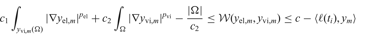
To start with, notice that the infimum in the incremental problems (22) is finite for every $i=1,\dots ,N_{\tau }$ . Indeed, since the initial condition satisfies $\mathcal{E}(0,y_{\mathrm{el}}^0,y_{\mathrm{vi}}^0)<\infty$ , by arguing by induction and choosing $(y_{\mathrm{el}},y_{\mathrm{vi}})=(y_{\mathrm{el}}^{i-1},y_{\mathrm{vi}}^{i-1})$ , we get that:

$$\mathcal{E}(t_i,y_{\mathrm{el}},y_{\mathrm{vi}})+\tau \mathrm{\Psi }(y_{\mathrm{vi}}^{i-1},\frac{y_{\mathrm{vi}}-y_{\mathrm{vi}}^{i-1}}{\tau })=\mathcal{E}(t_i,y_{\mathrm{el}}^{i-1},y_{\mathrm{vi}}^{i-1})<\infty .$$

Fix now $1\le i\le N$ and let $(y_{\mathrm{el},m}^i,y_{\mathrm{vi},m}^i{)}_{m\in \mathbb{N}}=(y_{\mathrm{el},m},y_{\mathrm{vi},m}{)}_{m\in \mathbb{N}}\subset \mathcal{A}$ be an infimizing sequence for problem (22) at time step $i$ .

5.1. Coercivity

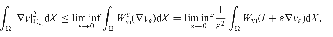
Let us first show that $(y_{\mathrm{el},m},y_{\mathrm{vi},m}{)}_{m\in \mathbb{N}}$ is bounded in $W^{1,p_{\mathrm{el}}}(y_{\mathrm{vi},m}(\mathrm{\Omega });{\mathbb{R}}^d)$ × $W^{1,p_{\mathrm{vi}}}(\mathrm{\Omega };{\mathbb{R}}^d)$ . This requires some care since $y_{\mathrm{el},m}$ is defined on the moving domain $y_{\mathrm{vi},m}(\mathrm{\Omega })$ . Since the infimum is finite, we have by equations (14) and (15):

$$c_1{\int }_{y_{\mathrm{vi},m}(\mathrm{\Omega })}|\nabla y_{\mathrm{el},m}{|}^{p_{\mathrm{el}}}+c_2{\int }_{\mathrm{\Omega }}|\nabla y_{\mathrm{vi},m}{|}^{p_{\mathrm{vi}}}-\frac{|\mathrm{\Omega }|}{c_2}\le \mathcal{W}(y_{\mathrm{el},m},y_{\mathrm{vi},m})\le c-〈\ell (t_i),y_m〉$$

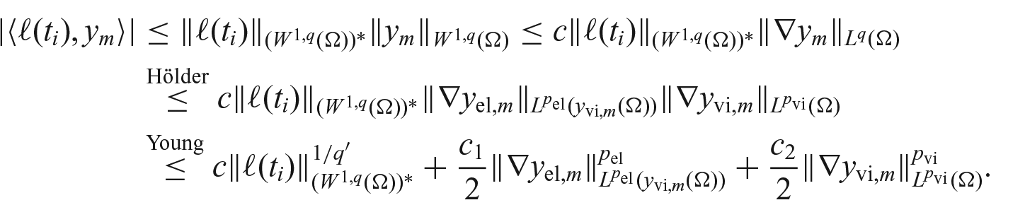
where we have posed $y_m:=y_{\mathrm{el},m}°y_{\mathrm{vi},m}$ . The loading term can be controlled as follows:

$$\begin{array}{c}|〈\ell (t_i),y_m〉|\le \parallel \ell (t_i){\parallel }_{{(W^{1,q}(\mathrm{\Omega }))}^{*}}\parallel y_m{\parallel }_{W^{1,q}(\mathrm{\Omega })}\le c\parallel \ell (t_i){\parallel }_{{(W^{1,q}(\mathrm{\Omega }))}^{*}}\parallel \nabla y_m{\parallel }_{L^q(\mathrm{\Omega })}\hfill \\ \stackrel{\mathrm{H}\stackrel{··}{\mathrm{o}}\mathrm{lder}}{\le }c\parallel \ell (t_i){\parallel }_{{(W^{1,q}(\mathrm{\Omega }))}^{*}}\parallel \nabla y_{\mathrm{el},m}{\parallel }_{L^{p_{\mathrm{el}}}(y_{\mathrm{vi},m}(\mathrm{\Omega }))}\parallel \nabla y_{\mathrm{vi},m}{\parallel }_{L^{p_{\mathrm{vi}}}(\mathrm{\Omega })}\hfill \\ \stackrel{\mathrm{Young}}{\le }c\parallel \ell (t_i){\parallel }_{{(W^{1,q}(\mathrm{\Omega }))}^{*}}^{1/q^{\prime }}+\frac{c_1}{2}\parallel \nabla y_{\mathrm{el},m}{\parallel }_{L^{p_{\mathrm{el}}}(y_{\mathrm{vi},m}(\mathrm{\Omega }))}^{p_{\mathrm{el}}}+\frac{c_2}{2}\parallel \nabla y_{\mathrm{vi},m}{\parallel }_{L^{p_{\mathrm{vi}}}(\mathrm{\Omega })}^{p_{\mathrm{vi}}}.\hfill \end{array}$$

This entails that:

$$\parallel \nabla y_{\mathrm{el},m}{\parallel }_{L^{p_{\mathrm{el}}}(y_{\mathrm{vi},m}(\mathrm{\Omega }))}^{p_{\mathrm{el}}}+\parallel \nabla y_{\mathrm{vi},m}{\parallel }_{L^{p_{\mathrm{vi}}}(\mathrm{\Omega })}^{p_{\mathrm{vi}}}\le c,$$

which in turn guarantees that:

$$\parallel \nabla y_m{\parallel }_{L^q(\mathrm{\Omega })}^q\le c.$$

Now, using the growth condition (15) and the Poincaré–Wirtinger inequality, recalling that $y_{\mathrm{vi}}$ has zero mean, we have that:

$$\parallel y_{\mathrm{vi},m}{\parallel }_{W^{1,p_{\mathrm{vi}}}(\mathrm{\Omega })}\le c.$$

Recalling that $y_m$ satisfies the Dirichlet boundary condition (13), by the Poincaré inequality, we obtain:

$$\parallel y_m{\parallel }_{W^{1,q}(\mathrm{\Omega })}\le c.$$

A change of variables ensures that:

$${\int }_{y_{\mathrm{vi},m}(\mathrm{\Omega })}|y_{\mathrm{el},m}{|}^{q}d\xi ={\int }_{\mathrm{\Omega }}|y_m{|}^q\mathrm{dX}\le c,$$

so that $\parallel y_{\mathrm{el},m}{\parallel }_{L^q(y_{\mathrm{vi},m}(\mathrm{\Omega }))}\le c$ , as well. Again the Poincaré inequality guarantees that:

$$\parallel y_{\mathrm{el},m}{\parallel }_{W^{1,p_{\mathrm{el}}}(y_{\mathrm{vi},m}(\mathrm{\Omega }))}\le c.$$

(39)

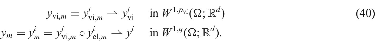
Up to a not relabeled subsequence, we hence have that:

$$\begin{array}{c}{y}_{\mathrm{vi},m}=y_{\mathrm{vi},m}^i\rightharpoonup y_{\mathrm{vi}}^i\mathrm{in}{W}^{1,p_{\mathrm{vi}}}(\mathrm{\Omega };{\mathbb{R}}^d)\hfill \\ y_m=y_m^i=y_{\mathrm{vi},m}^i°y_{\mathrm{el},m}^i\rightharpoonup y^i\mathrm{in}{W}^{1,q}(\mathrm{\Omega };{\mathbb{R}}^d).\hfill \end{array}$$

(40)

We now want to extract a converging subsequence from the elastic deformations $y_{\mathrm{el},m}$ , which are, however, defined on the moving domains $y_{\mathrm{vi},m}(\mathrm{\Omega })$ . Consider the trivial extensions $\overline{y_{\mathrm{el},m}}$ and $\overline{\nabla y_{\mathrm{el},m}}$ on the whole ${\mathbb{R}}^d$ by setting $y_{\mathrm{el},m}$ and $\nabla y_{\mathrm{el},m}$ to be zero on ${\mathbb{R}}^d\backslash y_{\mathrm{vi},m}(\mathrm{\Omega })$ , respectively. Recalling the bound (39), we have (up to a subsequence):

$$\begin{array}{c}\overline{y_{\mathrm{el},m}}\rightharpoonup y_{\mathrm{el}}^i\mathrm{in}{L}^{p_{\mathrm{el}}}({\mathbb{R}}^d;{\mathbb{R}}^d),\hfill \\ \overline{\nabla y_{\mathrm{el},m}}\rightharpoonup G\mathrm{in}{L}^{p_{\mathrm{el}}}({\mathbb{R}}^d;{\mathbb{R}}^{d\times d}).\hfill \end{array}$$

(41)

We want to show that $G=\nabla y_{\mathrm{el}}^i$ on the limiting set $y_{\mathrm{vi}}^i(\mathrm{\Omega })$ . By Sobolev embedding, possibly by extracting a further subsequence, we have that $y_{\mathrm{vi},m}\to y_{\mathrm{vi}}^i$ uniformly. Letting $\omega \subset \subset y_{\mathrm{vi}}^i(\mathrm{\Omega })$ , for $m$ large enough, we eventually have that $\omega \subset \subset y_{\mathrm{vi},m}(\mathrm{\Omega })$ . By uniqueness of the limit, we have $\overline{y_{\mathrm{el},m}}\rightharpoonup y_{\mathrm{el}}^i\mathrm{in}{L}^{p_{\mathrm{el}}}(\omega ;{\mathbb{R}}^d)$ and $\overline{\nabla y_{\mathrm{el},m}}\rightharpoonup \nabla y_{\mathrm{el}}^i=G\mathrm{in}{L}^{p_{\mathrm{el}}}(\omega ;{\mathbb{R}}^{d\times d})$ . Hence, $G=\nabla y_{\mathrm{el}}^i$ in every $\omega \subset \subset y_{\mathrm{vi}}^i(\mathrm{\Omega })$ . An exhaustion argument ensures that $G=\nabla y_{\mathrm{el}}^i$ in $y_{\mathrm{vi}}^i(\mathrm{\Omega })$ .

5.2. Closure of the set of admissible deformations

Let us now check that the weak limit $(y_{\mathrm{el}}^i,y_{\mathrm{vi}}^i)$ belongs to the admissible set $\mathcal{A}$ . First, since $p_{\mathrm{vi}}>d$ , we have that:

$$1=det\nabla y_{\mathrm{vi},m}^i\rightharpoonup det\nabla y_{\mathrm{vi}}^i\mathrm{in}{L}^{p_{\mathrm{vi}}/d}(\mathrm{\Omega }),$$

and hence $det\nabla y_{\mathrm{vi}}^i=1$ almost everywhere. On the contrary, Lemmas $3.1-3.2$ in Kruzík et al. [13] imply that $y_{\mathrm{vi}}^i(\mathrm{\Omega })\in {\mathcal{J}}_{{\eta }_1,{\eta }_2}$ . By the linearity of the mean and trace operators and by the weak convergence of $y_{\mathrm{vi},m}^i$ , we find ${\int }_{\mathrm{\Omega }}{y}_{\mathrm{vi}}^i\mathrm{d}X=0$ and $y^i=\mathrm{id}$ on ${\mathrm{\Gamma }}_D$ . Moreover, by Grandi et al. [39, Lemma 5.2(i)], we have that:

$$|y_{\mathrm{vi},m}^i(\mathrm{\Omega })\mathrm{\Delta }{y}_{\mathrm{vi}}^i(\mathrm{\Omega })|\to 0,$$

where the symbol $\mathrm{\Delta }$ denotes the symmetric difference, and, for every $\omega \subset \mathrm{\Omega }$ , that $1_{y_{\mathrm{vi},m}^i(\omega )}\to 1_{y_{\mathrm{vi}}^i(\omega )}$ almost everywhere in $\mathrm{\Omega }$ . This implies that $y_{\mathrm{vi}}^i$ satisfies the Ciarlet–Nečas condition, since:

$$|\mathrm{\Omega }|=|y_{\mathrm{vi},m}^i(\mathrm{\Omega })|\to |y_{\mathrm{vi}}^i(\mathrm{\Omega })|.$$

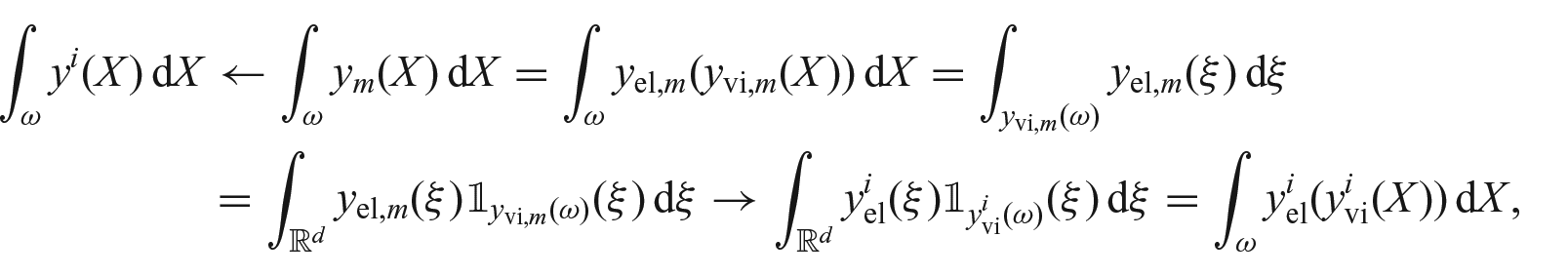
It remains to show that $y^i=y_{\mathrm{el}}^i°y_{\mathrm{vi}}^i$ . Let us take any measurable $\omega \subset \mathrm{\Omega }$ and consider, by changing variables,

$$\begin{array}{c}{\int }_{\omega }{y}^i(X)\mathrm{d}X\leftarrow {\int }_{\omega }{y}_m(X)\mathrm{d}X={\int }_{\omega }{y}_{\mathrm{el},m}(y_{\mathrm{vi},m}(X))\mathrm{d}X={\int }_{y_{\mathrm{vi},m}(\omega )}{y}_{\mathrm{el},m}(\xi )\mathrm{d}\xi \hfill \\ \multicolumn{1}{c}{={\int }_{{\mathbb{R}}^d}{y}_{\mathrm{el},m}(\xi )1_{y_{\mathrm{vi},m}(\omega )}(\xi )\mathrm{d}\xi \to {\int }_{{\mathbb{R}}^d}{y}_{\mathrm{el}}^i(\xi )1_{y_{\mathrm{vi}}^i(\omega )}(\xi )\mathrm{d}\xi ={\int }_{\omega }{y}_{\mathrm{el}}^i(y_{\mathrm{vi}}^i(X))\mathrm{d}X,}\end{array}$$

where, in the last limit, we used the weak convergence of $y_{\mathrm{el},m}$ and the strong convergence of $1_{y_{\mathrm{vi}}^i(\omega )}$ . Since $\omega \subset \mathrm{\Omega }$ is arbitrary, we conclude that $y^i=y_{\mathrm{el}}^i°y_{\mathrm{vi}}^i$ . In particular, we have that $(y_{\mathrm{el}}^i,y_{\mathrm{vi}}^i)\in \mathcal{A}$ .

5.3. Weak lower semicontinuity

We aim to show that the functional in equation (22) is weakly lower semicontinuous with respect to the above convergences.

By polyconvexity of the viscous energy density $W_{\mathrm{vi}}$ and equation (40), we have:

$${\int }_{\mathrm{\Omega }}{W}_{\mathrm{vi}}(\nabla y_{\mathrm{vi}}^i)\mathrm{dX}\le \underset{m\to \infty }{\lim \inf }{\int }_{\mathrm{\Omega }}{W}_{\mathrm{vi}}(\nabla y_{\mathrm{vi},m})\mathrm{dX}.$$

For what concerns the dissipation, from the weak convergence of $y_{\mathrm{vi},m}$ in $W^{1,p_{\mathrm{vi}}}(\mathrm{\Omega })$ , we also have:

$$\frac{\nabla (y_{\mathrm{vi},m}-y_{\mathrm{vi}}^{i-1})}{\tau }(\nabla y_{\mathrm{vi}}^{i-1}{)}^{-1}\rightharpoonup \frac{\nabla (y_{\mathrm{vi}}^i-y_{\mathrm{vi}}^{i-1})}{\tau }(\nabla y_{\mathrm{vi}}^{i-1}{)}^{-1}\mathrm{in}{L}^{p_{\psi }}(\mathrm{\Omega };{\mathbb{R}}^{d\times d}).$$

Hence, by the weak lower semicontinuity of $\mathrm{\Psi }$ , it follows that:

$$\mathrm{\Psi }(y_{\mathrm{vi}}^{i-1},\frac{y_{\mathrm{vi}}^i-y_{\mathrm{vi}}^{i-1}}{\tau })\le \underset{m\to \infty }{\lim \inf }\mathrm{\Psi }(y_{\mathrm{vi}}^{i-1},\frac{y_{\mathrm{vi},m}-y_{\mathrm{vi}}^{i-1}}{\tau }).$$

As the loading term is linear, we have:

$$〈\ell (t_i),y^i〉=\underset{m\to \infty }{\lim }〈\ell (t_i),y_m〉,$$

by weak convergence of $y_m$ .

Finally, for any $\omega \subset \subset y_{\mathrm{vi}}^i(\mathrm{\Omega })$ , we can treat the elastic energy as follows:

$${\int }_{\omega }{W}_{\mathrm{el}}(\nabla y_{\mathrm{el}}^i)\mathrm{d}\xi \le \underset{m\to \infty }{\lim \inf }{\int }_{\omega }{W}_{\mathrm{el}}(\nabla y_{\mathrm{el},m})\mathrm{d}\xi \stackrel{(14)}{\le }\underset{m\to \infty }{\lim \inf }{\int }_{y_{\mathrm{vi},m}(\mathrm{\Omega })}{W}_{\mathrm{el}}(\nabla y_{\mathrm{el},m})\mathrm{d}\xi ,$$

where we have used the polyconvexity of $W_{\mathrm{el}}$ and convergence (41). Taking the supremum over $\omega \subset \subset y_{\mathrm{vi}}^i(\mathrm{\Omega })$ , we conclude via an exhaustion argument that:

$${\int }_{y_{\mathrm{vi},m}(\mathrm{\Omega })}{W}_{\mathrm{el}}(\nabla y_{\mathrm{el}})\mathrm{d}\xi \le \underset{m\to \infty }{\lim \inf }{\int }_{y_{\mathrm{vi},m}(\mathrm{\Omega })}{W}_{\mathrm{el}}(\nabla y_{\mathrm{el},m})\mathrm{d}\xi .$$

All in all, we have proved that $(y_{\mathrm{el}}^i,y_{\mathrm{vi}}^i)\in \mathcal{A}$ and:

$$\mathcal{E}(t_i,y_{\mathrm{el}}^i,y_{\mathrm{vi}}^i)+\tau \mathrm{\Psi }(y_{\mathrm{vi}}^{i-1},\frac{y_{\mathrm{vi}}^i-y_{\mathrm{vi}}^{i-1}}{\tau })=\underset{(y_{\mathrm{el}},y_{\mathrm{vi}})\in \mathcal{A}}{min}\{\mathcal{E}(t_i,y_{\mathrm{el}},y_{\mathrm{vi}})+\tau \mathrm{\Psi }(y_{\mathrm{vi}}^{i-1},\frac{y_{\mathrm{vi}}-y_{\mathrm{vi}}^{i-1}}{\tau })\},$$

so that the assertion of Proposition 4.1 follows.

6. Existence of approximable solutions: Proof of Theorem 4.1

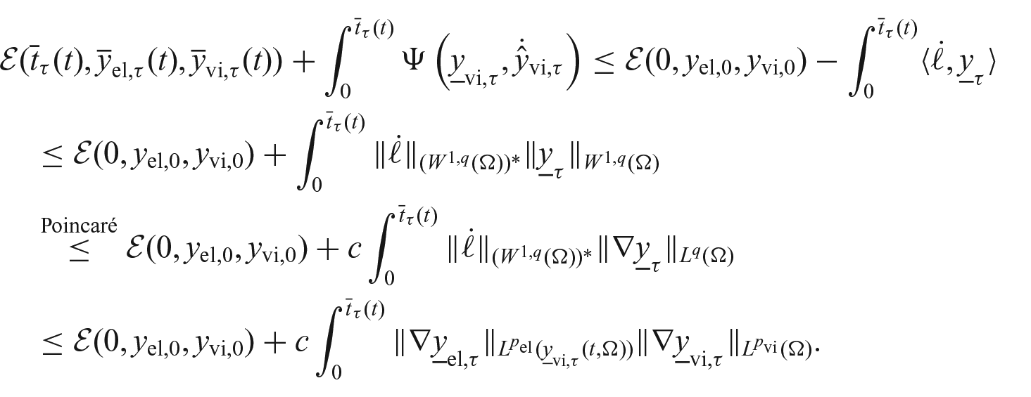
We split the proof in subsequent steps. The basic energy estimate and its consequences are presented in section 6.1. The energy estimate is then sharpened in section 6.2, leading to the discrete energy inequality. By taking limits as the time step $\tau$ goes to $0$ , the time-continuous energy inequality (23) and the time-continuous semistability (24) are proved in sections 6.3 and 6.4, respectively.

6.1. Energy estimate and its consequences

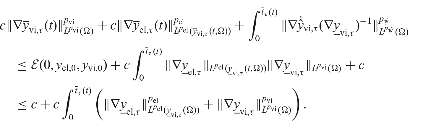
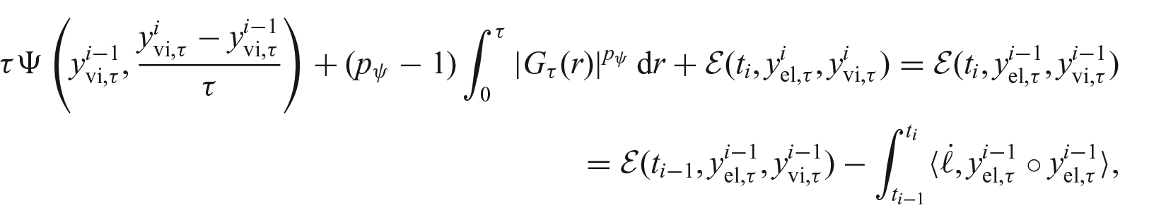
Let $(y_{\mathrm{el}}^i{y}_{\mathrm{vi}}^i{)}_{i=0}^N$ be a solution to equation (22). By minimality, we have, for every $i=1,...,N$ ,

$$\begin{array}{c}\mathcal{E}(t_i,y_{\mathrm{el}}^i,y_{\mathrm{vi}}^i)+\tau \mathrm{\Psi }(y_{\mathrm{vi}}^{i-1},\frac{y_{\mathrm{vi}}^i-y_{\mathrm{vi}}^{i-1}}{\tau })\le \mathcal{E}(t_i,y_{\mathrm{el}}^{i-1},y_{\mathrm{vi}}^{i-1})\hfill \\ \multicolumn{1}{c}{=\mathcal{E}(t_{i-1},y_{\mathrm{el}}^{i-1},y_{\mathrm{vi}}^{i-1})-{\int }_{t_{i-1}}^{t_i}〈\stackrel{·}{\ell },y^{i-1}〉.}\end{array}$$

Summing up over $i=1,...,n\le N$ , we get:

$$\mathcal{E}(t_n,y_{\mathrm{el}}^n,y_{\mathrm{vi}}^n)+\sum _{i=1}^n\tau \mathrm{\Psi }(y_{\mathrm{vi}}^{i-1},\frac{y_{\mathrm{vi}}^i-y_{\mathrm{vi}}^{i-1}}{\tau })\le \mathcal{E}(0,y_{\mathrm{el},0},y_{\mathrm{vi},0})-\sum _{i=1}^n{\int }_{t_{i-1}}^{t_i}〈\stackrel{·}{\ell },y^{i-1}〉.$$

(42)

Using the notation for the interpolants, we have, for all $t\in [0,T],$

$$\begin{array}{c}\mathcal{E}({\overline{t}}_{\tau }(t),{\overline{y}}_{\mathrm{el},\tau }(t),{\overline{y}}_{\mathrm{vi},\tau }(t))+{\int }_0^{{\overline{t}}_{\tau }(t)}\mathrm{\Psi }({\underset{¯}{y}}_{\mathrm{vi},\tau },{\stackrel{·}{\hat{y}}}_{\mathrm{vi},\tau })\le \mathcal{E}(0,y_{\mathrm{el},0},y_{\mathrm{vi},0})-{\int }_0^{{\overline{t}}_{\tau }(t)}〈\stackrel{·}{\ell },{\underset{¯}{y}}_{\tau }〉\hfill \\ \le \mathcal{E}(0,y_{\mathrm{el},0},y_{\mathrm{vi},0})+{\int }_0^{{\overline{t}}_{\tau }(t)}\parallel \stackrel{·}{\ell }{\parallel }_{{(W^{1,q}(\mathrm{\Omega }))}^{*}}\parallel {\underset{¯}{y}}_{\tau }{\parallel }_{W^{1,q}(\mathrm{\Omega })}\hfill \\ \stackrel{\mathrm{Poincar}é}{\le }\mathcal{E}(0,y_{\mathrm{el},0},y_{\mathrm{vi},0})+c{\int }_0^{{\overline{t}}_{\tau }(t)}\parallel \stackrel{·}{\ell }{\parallel }_{{(W^{1,q}(\mathrm{\Omega }))}^{*}}\parallel \nabla {\underset{¯}{y}}_{\tau }{\parallel }_{L^q(\mathrm{\Omega })}\hfill \\ \le \mathcal{E}(0,y_{\mathrm{el},0},y_{\mathrm{vi},0})+c{\int }_0^{{\overline{t}}_{\tau }(t)}\parallel \nabla {\underset{¯}{y}}_{\mathrm{el},\tau }{\parallel }_{L^{p_{\mathrm{el}}}({\underset{¯}{y}}_{\mathrm{vi},\tau }(t,\mathrm{\Omega }))}\parallel \nabla {\underset{¯}{y}}_{\mathrm{vi},\tau }{\parallel }_{L^{p_{\mathrm{vi}}}(\mathrm{\Omega })}.\hfill \end{array}$$

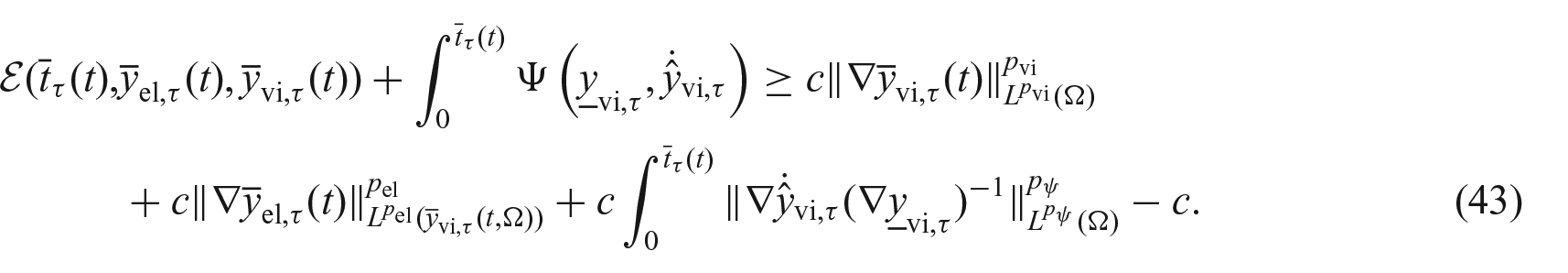
On the contrary, by the growth assumptions (14), (15), and (18), we also have:

$$\begin{array}{c}\mathcal{E}({\overline{t}}_{\tau }(t),{\overline{y}}_{\mathrm{el},\tau }(t),{\overline{y}}_{\mathrm{vi},\tau }(t))+{\int }_0^{{\overline{t}}_{\tau }(t)}\mathrm{\Psi }({\underset{¯}{y}}_{\mathrm{vi},\tau },{\stackrel{·}{\hat{y}}}_{\mathrm{vi},\tau })\ge c\parallel \nabla {\overline{y}}_{\mathrm{vi},\tau }(t){\parallel }_{L^{p_{\mathrm{vi}}}(\mathrm{\Omega })}^{p_{\mathrm{vi}}}\hfill \\ +c\parallel \nabla {\overline{y}}_{\mathrm{el},\tau }(t){\parallel }_{L^{p_{\mathrm{el}}}({\overline{y}}_{\mathrm{vi},\tau }(t,\mathrm{\Omega }))}^{p_{\mathrm{el}}}+c{\int }_0^{{\overline{t}}_{\tau }(t)}\parallel \nabla {\stackrel{·}{\hat{y}}}_{\mathrm{vi},\tau }(\nabla {\underset{¯}{y}}_{\mathrm{vi},\tau }{)}^{-1}{\parallel }_{L^{p_{\psi }}(\mathrm{\Omega })}^{p_{\psi }}-c.\hfill \end{array}$$

(43)

In particular, by combining the above two inequalities, we get:

$$\begin{array}{c}c\parallel \nabla {\overline{y}}_{\mathrm{vi},\tau }(t){\parallel }_{L^{p_{\mathrm{vi}}}(\mathrm{\Omega })}^{p_{\mathrm{vi}}}+c\parallel \nabla {\overline{y}}_{\mathrm{el},\tau }(t){\parallel }_{L^{p_{\mathrm{el}}}({\overline{y}}_{\mathrm{vi},\tau }(t,\mathrm{\Omega }))}^{p_{\mathrm{el}}}+{\int }_0^{{\overline{t}}_{\tau }(t)}\parallel \nabla {\stackrel{·}{\hat{y}}}_{\mathrm{vi},\tau }{(\nabla {\underset{¯}{y}}_{\mathrm{vi},\tau })}^{-1}{\parallel }_{L^{p_{\psi }}(\mathrm{\Omega })}^{p_{\psi }}\hfill \\ \multicolumn{1}{c}{\le \mathcal{E}(0,y_{\mathrm{el},0},y_{\mathrm{vi},0})+c{\int }_0^{{\overline{t}}_{\tau }(t)}\parallel \nabla {\underset{¯}{y}}_{\mathrm{el},\tau }{\parallel }_{L^{p_{\mathrm{el}}}({\underset{¯}{y}}_{\mathrm{vi},\tau }(t,\mathrm{\Omega }))}\parallel \nabla {\underset{¯}{y}}_{\mathrm{vi},\tau }{\parallel }_{L^{p_{\mathrm{vi}}}(\mathrm{\Omega })}+c}\\ \multicolumn{1}{c}{\le c+c{\int }_0^{{\overline{t}}_{\tau }(t)}(\parallel \nabla {\underset{¯}{y}}_{\mathrm{el},\tau }{\parallel }_{L^{p_{\mathrm{el}}}({\underset{¯}{y}}_{\mathrm{vi},\tau }(\mathrm{\Omega }))}^{p_{\mathrm{el}}}+\parallel \nabla {\underset{¯}{y}}_{\mathrm{vi},\tau }{\parallel }_{L^{p_{\mathrm{vi}}}(\mathrm{\Omega })}^{p_{\mathrm{vi}}}).}\end{array}$$

We can apply the Discrete Gronwall Lemma [3, (C.2.6), p. 534] to find:

$$\parallel \nabla {\overline{y}}_{\mathrm{vi},\tau }(t){\parallel }_{L^{p_{\mathrm{vi}}}(\mathrm{\Omega })}+\parallel \nabla {\overline{y}}_{\mathrm{el},\tau }(t){\parallel }_{L^{p_{\mathrm{el}}}({\overline{y}}_{\mathrm{vi},\tau }(\mathrm{\Omega }))}\le c.$$

Thus, for every $t\in [0,T]$ , we have:

$$\parallel {\overline{y}}_{\mathrm{vi},\tau }(t){\parallel }_{W^{1,p_{\mathrm{vi}}}(\mathrm{\Omega })}\le c\mathrm{and}\parallel \nabla {\overline{y}}_{\mathrm{el},\tau }(t){\parallel }_{L^{p_{\mathrm{el}}}({\overline{y}}_{\mathrm{vi},\tau }(t,\mathrm{\Omega }))}\le c.$$

Then, using the Poincaré inequality on the total deformation, we find $\parallel {\overline{y}}_{\tau }(t){\parallel }_{W^{1,q}(\mathrm{\Omega })}\le c$ and hence, as before, for every $t\in [0,T]$ :

$$\parallel {\overline{y}}_{\mathrm{el},\tau }(t){\parallel }_{W^{1,p_{\mathrm{el}}}({\overline{y}}_{\mathrm{vi},\tau }(t,\mathrm{\Omega }))}\le c.$$

Moreover, thanks to equation (43), we also have for every $t\in [0,T]$ :

$${\int }_0^{{\overline{t}}_{\tau }(t)}\parallel \nabla {\stackrel{·}{\hat{y}}}_{\mathrm{vi},\tau }(\nabla {\underset{¯}{y}}_{\mathrm{vi},\tau }{)}^{-1}{\parallel }_{L^{p_{\psi }}(\mathrm{\Omega })}^{p_{\psi }}\le c.$$

(44)

By recalling that $1/p_r=1/p_{\psi }+1/p_{\mathrm{vi}}$ , this implies that:

$${\int }_0^T\parallel \nabla {\stackrel{·}{\hat{y}}}_{\mathrm{vi},\tau }{\parallel }_{L^{p_r}(\mathrm{\Omega })}\le {\int }_0^T\parallel \nabla {\stackrel{·}{\hat{y}}}_{\mathrm{vi},\tau }(\nabla {\underset{¯}{y}}_{\mathrm{vi},\tau }{)}^{-1}{\parallel }_{L^{p_{\psi }}(\mathrm{\Omega })}\parallel \nabla {\underset{¯}{y}}_{\mathrm{vi},\tau }{\parallel }_{L^{p_{\mathrm{vi}}}(\mathrm{\Omega })}\le c.$$

6.2. Energy inequality, sharp version

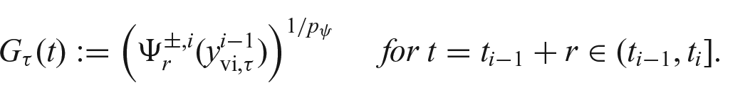
In the previous section, we have found the energy estimate (42), which features the dissipation with a prefactor $1$ . In order to prove the sharp version of the energy inequality (23) with the prefactor $p_{\psi }$ , we need a finer argument, mutated from Ambrosio et al. [30].

First, we introduce some notation. Let:

$$\mathcal{V}=\{y_{\mathrm{vi}}\in W^{1,p_{\mathrm{vi}}}(\mathrm{\Omega };{\mathbb{R}}^d)|det\nabla y_{\mathrm{vi}}=1\mathrm{a}.\mathrm{e}.\mathrm{in}\mathrm{\Omega }\},$$

and, for all $i=1,\dots ,N$ , define the functionals ${\mathrm{\Phi }}^i:[0,T]\times \mathcal{V}\times \mathcal{A}\to \mathbb{R}$ as:

$${\mathrm{\Phi }}^i(\tau ;y_{\mathrm{old}},y_{\mathrm{el}},y_{\mathrm{vi}}):=\mathcal{E}(t_i,y_{\mathrm{el}},y_{\mathrm{vi}})+\tau \mathrm{\Psi }(y_{\mathrm{old}},\frac{y_{\mathrm{vi}}-y_{\mathrm{old}}}{\tau }).$$

Recall that, by definition (17) of $\mathrm{\Psi }$ and by the $p_{\psi }$ -homogeneity (19), we have:

$$\tau \mathrm{\Psi }(y_{\mathrm{old}},\frac{y_{\mathrm{vi}}-y_{\mathrm{old}}}{\tau })=\frac{1}{{\tau }^{p_{\psi }-1}}{\int }_{\mathrm{\Omega }}\psi ({(\nabla y_{\mathrm{old}})}^{-1}(\nabla y_{\mathrm{vi}}-\nabla y_{\mathrm{old}})).$$

(45)

For all $(t,y_{\mathrm{old}})\in [0,T]\times \mathcal{V}$ , we also define the minimal value of the latter functional as:

$${\varphi }_{\tau }^i(y_{\mathrm{old}}):=\underset{(y_{\mathrm{el}},y_{\mathrm{vi}})\in \mathcal{A}}{inf}{\mathrm{\Phi }}^i(\tau ;y_{\mathrm{old}},y_{\mathrm{el}},y_{\mathrm{vi}}),$$

and denote the set of minimizers by $J_{\tau }^i(y_{\mathrm{old}}):=\arg \min \{{\mathrm{\Phi }}^i(\tau ;y_{\mathrm{old}},y_{\mathrm{el}},y_{\mathrm{vi}})|(y_{\mathrm{el}},y_{\mathrm{vi}})\in \mathcal{A}\}$ , which is nonempty by Proposition 4.1. Finally, introduce:

$$\begin{array}{c}{\mathrm{\Psi }}_{\tau }^{+,i}(y_{\mathrm{old}}):=\underset{(y_{\mathrm{el},\tau },y_{\mathrm{vi},\tau })\in J_{\tau }^i(y_{\mathrm{old}})}{sup}{\int }_{\mathrm{\Omega }}\psi \left({(\nabla y_{\mathrm{old}})}^{-1}\frac{(\nabla y_{\mathrm{vi},\tau }-\nabla y_{\mathrm{old}})}{\tau }\right),\hfill \\ {\mathrm{\Psi }}_{\tau }^{-,i}(y_{\mathrm{old}}):=\underset{(y_{\mathrm{el},\tau },y_{\mathrm{vi},\tau })\in J_{\tau }^i(y_{\mathrm{old}})}{inf}{\int }_{\mathrm{\Omega }}\psi \left({(\nabla y_{\mathrm{old}})}^{-1}\frac{(\nabla y_{\mathrm{vi},\tau }-\nabla y_{\mathrm{old}})}{\tau }\right).\hfill \end{array}$$

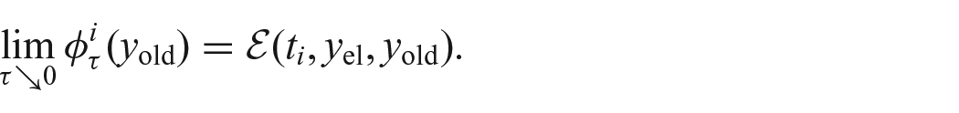
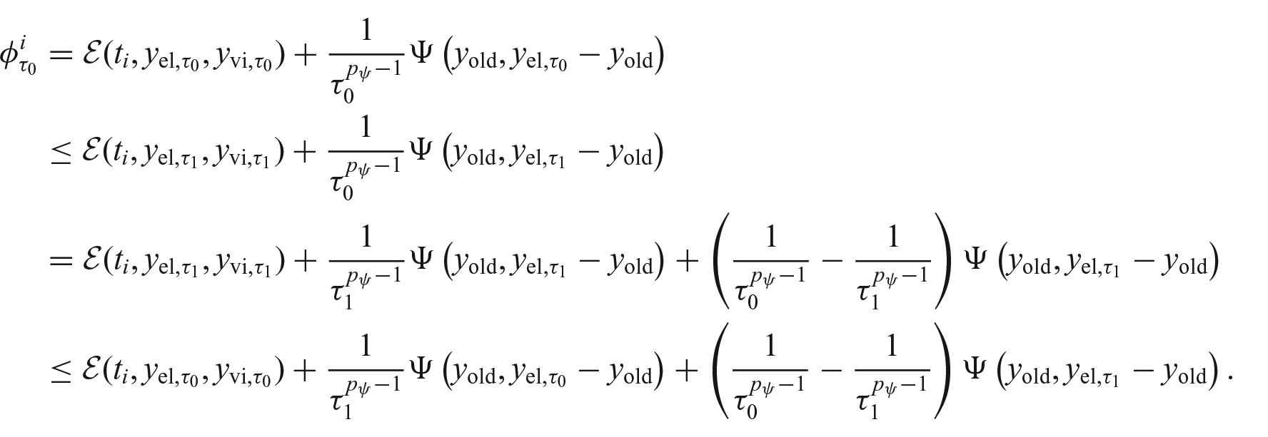
We start by stating an auxiliary result, providing the continuity property of the map $\tau \to {\varphi }_{\tau }^i(y_{\mathrm{old}})$ in $0$ and the monotonicity of $\tau \to \mathrm{\Psi }(y_{\mathrm{old}},y_{\mathrm{vi},\tau }-y_{\mathrm{old}})$ .

Lemma 6.1. For every $i=1,\dots ,N$ and every $y_{\mathrm{old}}\in \mathcal{V}$ , we have:

$$\underset{\tau \searrow 0}{\lim }{\varphi }_{\tau }^i(y_{\mathrm{old}})=\mathcal{E}(t_i,y_{\mathrm{el}},y_{\mathrm{old}}),$$

(46)

where $y_{\mathrm{el}}\in \arg \min \{\mathcal{E}(t_i,{\tilde{y}}_{\mathrm{el}},y_{\mathrm{old}})|{\tilde{y}}_{\mathrm{el}}\in W^{1,p_{\mathrm{el}}}(y_{\mathrm{old}}(\mathrm{\Omega });{\mathbb{R}}^d)\}$ .

Moreover, if $0<{\tau }_0<{\tau }_1$ , then:

$$\mathrm{\Psi }(y_{\mathrm{old}},y_{\mathrm{vi},{\tau }_0}-y_{\mathrm{old}})\le \mathrm{\Psi }(y_{\mathrm{old}},y_{\mathrm{vi},{\tau }_1}-y_{\mathrm{old}})\mathrm{for}\mathrm{every}(y_{\mathrm{el},{\tau }_j},y_{\mathrm{vi},{\tau }_j})\in J_{{\tau }_j}^i(y_{\mathrm{old}}),j=0,1.$$

(47)

Proof. We start by proving the continuity property of $\tau \mapsto {\varphi }_{\tau }^i(y_{\mathrm{old}})$ . Let $(y_{\mathrm{el},\tau },y_{\mathrm{vi},\tau })\in J_{\tau }^i(y_{\mathrm{old}})$ . By the growth condition (18), the $p_{\psi }$ -homogeneity (19), and coercivity, we have:

$$\parallel (\nabla y_{\mathrm{old}}{)}^{-1}(\nabla y_{\mathrm{vi},\tau }-\nabla y_{\mathrm{old}}){\parallel }_{L^{p_{\mathrm{vi}}}(\mathrm{\Omega })}\le c\mathrm{\Psi }(y_{\mathrm{old}},y_{\mathrm{vi},\tau }-y_{\mathrm{old}})=c{\tau }^{p_{\psi }}\mathrm{\Psi }(y_{\mathrm{old}},\frac{y_{\mathrm{vi},\tau }-y_{\mathrm{old}}}{\tau })\le c{\tau }^{p_{\psi }-1}.$$

This proves that $\nabla y_{\mathrm{vi},\tau }\to \nabla y_{\mathrm{old}}$ in $L^{p_{\mathrm{vi}}}(\mathrm{\Omega };{\mathbb{R}}^{d\times d})$ as $\tau \to 0$ . Moreover, by equation (39), we have $y_{\mathrm{el},\tau }\rightharpoonup y_{\mathrm{el}}$ weakly in $W^{1,p_{\mathrm{el}}}(\mathrm{\Omega };{\mathbb{R}}^d)$ . Thus, by weak lower semicontinuity, we have:

$$\underset{\tau \searrow 0}{\lim }{\varphi }_{\tau }^i(y_{\mathrm{old}})=\underset{\tau \searrow 0}{\lim }{\mathrm{\Phi }}^i(\tau ;y_{\mathrm{old}},y_{\mathrm{el},\tau },y_{\mathrm{vi},\tau })\ge \underset{\tau \searrow 0}{\lim \inf }\mathcal{E}(t_i,y_{\mathrm{el},\tau },y_{\mathrm{vi},\tau })\ge \mathcal{E}(t_i,y_{\mathrm{el}},y_{\mathrm{old}}).$$

On the contrary, from minimality, we get $\mathcal{E}(t_i,y_{\mathrm{el}},y_{\mathrm{old}})\ge {\varphi }_{\tau }^i(y_{\mathrm{old}})$ . This implies that:

$$\underset{\tau \searrow 0}{\lim }{\varphi }_{\tau }^i(y_{\mathrm{old}})=\mathcal{E}(t_i,y_{\mathrm{el}},y_{\mathrm{old}}).$$

The fact that $y_{\mathrm{el}}\in \arg \min \{\mathcal{E}(t_i,{\tilde{y}}_{\mathrm{el}},y_{\mathrm{old}})|{\tilde{y}}_{\mathrm{el}}\in W^{1,p_{\mathrm{el}}}(y_{\mathrm{old}}(\mathrm{\Omega });{\mathbb{R}}^d)\}$ follows from minimality since:

$$\mathcal{E}(t_i,y_{\mathrm{el}},y_{\mathrm{old}})=\underset{\tau \searrow 0}{\lim }{\varphi }_{\tau }^i(y_{\mathrm{old}})\le \underset{\tau \searrow 0}{\lim }{\mathrm{\Phi }}^i(\tau ;y_{\mathrm{old}},{\tilde{y}}_{\mathrm{el}},y_{\mathrm{old}})=\mathcal{E}(t_i,{\tilde{y}}_{\mathrm{el}},y_{\mathrm{old}}),$$

for every ${\tilde{y}}_{\mathrm{el}}\in W^{1,p_{\mathrm{el}}}(y_{\mathrm{old}}(\mathrm{\Omega });{\mathbb{R}}^d)$ .

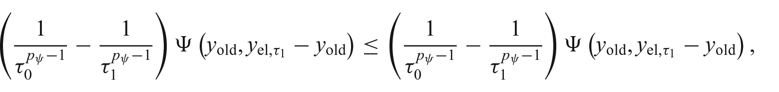
Let us now prove the monotonicity of $\tau \to \mathrm{\Psi }(y_{\mathrm{old}},y_{\mathrm{vi},\tau }-y_{\mathrm{old}})$ . Let $0<{\tau }_0<{\tau }_1$ and $y_{\mathrm{el},{\tau }_j},y_{\mathrm{vi},{\tau }_j}\in J_{{\tau }_j}^i(y_{\mathrm{old}})$ , $j=0,1$ . From minimality, we have that:

$$\begin{array}{c}{\varphi }_{{\tau }_0}^i=\mathcal{E}(t_i,y_{\mathrm{el},{\tau }_0},y_{\mathrm{vi},{\tau }_0})+\frac{1}{{\tau }_0^{p_{\psi }-1}}\mathrm{\Psi }(y_{\mathrm{old}},y_{\mathrm{el},{\tau }_0}-y_{\mathrm{old}})\hfill \\ \le \mathcal{E}(t_i,y_{\mathrm{el},{\tau }_1},y_{\mathrm{vi},{\tau }_1})+\frac{1}{{\tau }_0^{p_{\psi }-1}}\mathrm{\Psi }(y_{\mathrm{old}},y_{\mathrm{el},{\tau }_1}-y_{\mathrm{old}})\hfill \\ =\mathcal{E}(t_i,y_{\mathrm{el},{\tau }_1},y_{\mathrm{vi},{\tau }_1})+\frac{1}{{\tau }_1^{p_{\psi }-1}}\mathrm{\Psi }(y_{\mathrm{old}},y_{\mathrm{el},{\tau }_1}-y_{\mathrm{old}})+(\frac{1}{{\tau }_0^{p_{\psi }-1}}-\frac{1}{{\tau }_1^{p_{\psi }-1}})\mathrm{\Psi }(y_{\mathrm{old}},y_{\mathrm{el},{\tau }_1}-y_{\mathrm{old}})\hfill \\ \le \mathcal{E}(t_i,y_{\mathrm{el},{\tau }_0},y_{\mathrm{vi},{\tau }_0})+\frac{1}{{\tau }_1^{p_{\psi }-1}}\mathrm{\Psi }(y_{\mathrm{old}},y_{\mathrm{el},{\tau }_0}-y_{\mathrm{old}})+(\frac{1}{{\tau }_0^{p_{\psi }-1}}-\frac{1}{{\tau }_1^{p_{\psi }-1}})\mathrm{\Psi }(y_{\mathrm{old}},y_{\mathrm{el},{\tau }_1}-y_{\mathrm{old}}).\hfill \end{array}$$

This implies that:

$$(\frac{1}{{\tau }_0^{p_{\psi }-1}}-\frac{1}{{\tau }_1^{p_{\psi }-1}})\mathrm{\Psi }(y_{\mathrm{old}},y_{\mathrm{el},{\tau }_1}-y_{\mathrm{old}})\le (\frac{1}{{\tau }_0^{p_{\psi }-1}}-\frac{1}{{\tau }_1^{p_{\psi }-1}})\mathrm{\Psi }(y_{\mathrm{old}},y_{\mathrm{el},{\tau }_1}-y_{\mathrm{old}}),$$

which concludes the proof.  □

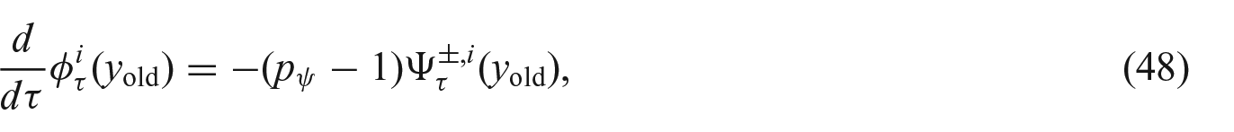
In the following Lemma, we calculate the derivative with respect to $\tau$ of the minimal incremental energy ${\varphi }_{\tau }^i$ and provide a crucial estimate.

Lemma 6.2. For every $y_{\mathrm{old}}\in \mathcal{V}$ and $i=1,\dots N$ , the map $\tau \mapsto {\varphi }_{\tau }^i(y_{\mathrm{old}})$ is locally Lipschitz on $(0,1)$ . Moreover, we have:

$$\frac{d}{d\tau }{\varphi }_{\tau }^i(y_{\mathrm{old}})=-(p_{\psi }-1){\mathrm{\Psi }}_{\tau }^{\pm ,i}(y_{\mathrm{old}}),$$

(48)

for almost every $\tau \in (0,1).$ In particular, for almost every $\tau \in (0,1)$ , we have:

$$\tau \mathrm{\Psi }(y_{\mathrm{old}},\frac{y_{\mathrm{vi},\tau }-y_{\mathrm{old}}}{\tau })+(p_{\psi }-1){\int }_0^{\tau }{\mathrm{\Psi }}_r^{\pm ,i}(y_{\mathrm{old}})\mathrm{dr}=\mathcal{E}(t_i,y_{\mathrm{el}},y_{\mathrm{old}})-\mathcal{E}(t_i,y_{\mathrm{el},\tau },y_{\mathrm{vi},\tau }),$$

(49)

for every $(y_{\mathrm{el},\tau },y_{\mathrm{vi},\tau })\in J_{\tau }^i(y_{\mathrm{old}})$ , for some $y_{\mathrm{el}}=\arg \min \{\mathcal{E}(t_i,{\tilde{y}}_{\mathrm{el}},y_{\mathrm{old}})|{\tilde{y}}_{\mathrm{el}}\in W^{1,p_{\mathrm{el}}}(y_{\mathrm{old}}(\mathrm{\Omega });{\mathbb{R}}^d)\}$ .

Proof. For every ${\tau }_0\ne {\tau }_1$ and $(y_{\mathrm{el},{\tau }_j},y_{\mathrm{vi},{\tau }_j})\in J_{{\tau }_j}^i(y_{\mathrm{old}})$ , $j=0,1$ , by minimality we have:

$$\begin{array}{c}{\varphi }_{{\tau }_0}(y_{\mathrm{old}})-{\varphi }_{{\tau }_1}(y_{\mathrm{old}})\le {\mathrm{\Phi }}^i({\tau }_0;y_{\mathrm{old}},y_{\mathrm{el},{\tau }_1},y_{\mathrm{vi},{\tau }_1})-{\mathrm{\Phi }}^i({\tau }_1;y_{\mathrm{old}},y_{\mathrm{el},{\tau }_1},y_{\mathrm{vi},{\tau }_1})\hfill \\ =\frac{1}{{\tau }_0^{p_{\psi }-1}}\mathrm{\Psi }(y_{\mathrm{old}},y_{\mathrm{vi},{\tau }_1}-y_{\mathrm{old}})-\frac{1}{{\tau }_1^{p_{\psi }-1}}\mathrm{\Psi }(y_{\mathrm{old}},y_{\mathrm{vi},{\tau }_1}-y_{\mathrm{old}})\hfill \\ =\frac{{\tau }_1^{p_{\psi }-1}-{\tau }_0^{p_{\psi }-1}}{{({\tau }_1{\tau }_0)}^{p_{\psi }-1}}{\int }_{\mathrm{\Omega }}\psi ({(\nabla y_{\mathrm{old}})}^{-1}(\nabla y_{\mathrm{vi},{\tau }_1}-\nabla y_{\mathrm{old}})),\hfill \end{array}$$

where we used equation (45). We can perform an analogous calculation for:

$${\varphi }_{{\tau }_0}(y_{\mathrm{old}})-{\varphi }_{{\tau }_1}(y_{\mathrm{old}})\ge {\mathrm{\Phi }}^i({\tau }_0;y_{\mathrm{old}},y_{\mathrm{el},{\tau }_0},y_{\mathrm{vi},{\tau }_0})-{\mathrm{\Phi }}^i({\tau }_1;y_{\mathrm{old}},y_{\mathrm{el},{\tau }_0},y_{\mathrm{vi},{\tau }_0}),$$

so that, by combining the two above inequalities, for ${\tau }_0<{\tau }_1$ we find:

$$\begin{array}{c}\frac{{\tau }_1^{p_{\psi }-1}-{\tau }_0^{p_{\psi }-1}}{{({\tau }_1{\tau }_0)}^{p_{\psi }-1}({\tau }_1-{\tau }_0)}{\int }_{\mathrm{\Omega }}\psi ({(\nabla y_{\mathrm{old}})}^{-1}(\nabla y_{\mathrm{vi},{\tau }_0}-\nabla y_{\mathrm{old}}))\le \frac{{\varphi }_{{\tau }_0}(y_{\mathrm{old}})-{\varphi }_{{\tau }_1}(y_{\mathrm{old}})}{{\tau }_1-{\tau }_0}\hfill \\ \le \frac{{\tau }_1^{p_{\psi }-1}-{\tau }_0^{p_{\psi }-1}}{{({\tau }_1{\tau }_0)}^{p_{\psi }-1}({\tau }_1-{\tau }_0)}{\int }_{\mathrm{\Omega }}\psi ({(\nabla y_{\mathrm{old}})}^{-1}(\nabla y_{\mathrm{vi},{\tau }_1}-\nabla y_{\mathrm{old}})).\hfill \end{array}$$

Taking the supremum over $(y_{\mathrm{el},{\tau }_0},y_{\mathrm{vi},{\tau }_0})\in J_{{\tau }_0}^i(y_{\mathrm{old}})$ in the left-hand side and the infimum over $(y_{\mathrm{el},{\tau }_1},y_{\mathrm{vi},{\tau }_1})\in J_{{\tau }_1}^i(y_{\mathrm{old}})$ in the right-hand side, we find:

$$\frac{{\tau }_0({\tau }_1^{p_{\psi }-1}-{\tau }_0^{p_{\psi }-1})}{{\tau }_1^{p_{\psi }-1}({\tau }_1-{\tau }_0)}{\mathrm{\Psi }}_{{\tau }_0}^{+,i}(y_{\mathrm{old}})\le \frac{{\varphi }_{{\tau }_0}(y_{\mathrm{old}})-{\varphi }_{{\tau }_1}(y_{\mathrm{old}})}{{\tau }_1-{\tau }_0}\le \frac{{\tau }_1({\tau }_1^{p_{\psi }-1}-{\tau }_0^{p_{\psi }-1})}{{\tau }_0^{p_{\psi }-1}({\tau }_1-{\tau }_0)}{\mathrm{\Psi }}_{{\tau }_1}^{-,i}(y_{\mathrm{old}}),$$

which implies that $\tau \to {\varphi }_{\tau }^i(y_{\mathrm{old}})$ is locally Lipschitz. Then, passing to the limit for ${\tau }_1\searrow \tau$ and ${\tau }_0\nearrow \tau$ , we get equation (48).

Integrating equation (48) from ${\tau }_0>0$ to $\tau$ , we have:

$${\varphi }_{\tau }^i(y_{\mathrm{old}})-{\varphi }_{{\tau }_0}^i(y_{\mathrm{old}})=-(p_{\psi }-1){\int }_{{\tau }_0}^{\tau }{\mathrm{\Psi }}_r^{\pm ,i}(y_{\mathrm{old}})\mathrm{dr}.$$

Letting ${\tau }_0\searrow 0$ , recalling equation (46), and the definition of $(y_{\mathrm{el},\tau },y_{\mathrm{vi},\tau })\in J_{\tau }^i(y_{\mathrm{old}})$ , we get equation (49).  □

We now state the definition of De Giorgi variational interpolation [30, Definition 3.2.1], which in our setting refers to the viscous deformation $y_{\mathrm{vi}}$ only.

Definition 6.1. (De Giorgi variational interpolation) Let $(y_{\mathrm{el},\tau }^i,y_{\mathrm{vi},\tau }^i{)}_{i=0}^N$ be an incremental solution of the problem of equation (22). We call De Giorgi variational interpolation of $(y_{\mathrm{vi},\tau }^i{)}_{i=0}^N$ any interpolation ${\tilde{y}}_{\mathrm{vi},\tau }$ of the discrete values with $({\overline{y}}_{\mathrm{el},\tau },{\tilde{y}}_{\mathrm{vi},\tau }):[0,T]\to \mathcal{A}$ that satisfies:

$${\tilde{y}}_{\mathrm{vi},\tau }(t)={\tilde{y}}_{\mathrm{vi},\tau }(t_{i-1}+r)\in J_r({\tilde{y}}_{\mathrm{vi},\tau }^{i-1})\mathrm{if}{t}_{i-1}+r\in (t_{i-1},t_i],$$

for every $i=1,\dots ,N$ .

The following proposition provides the sharp energy estimate on the discrete level, providing an equality instead of an inequality.

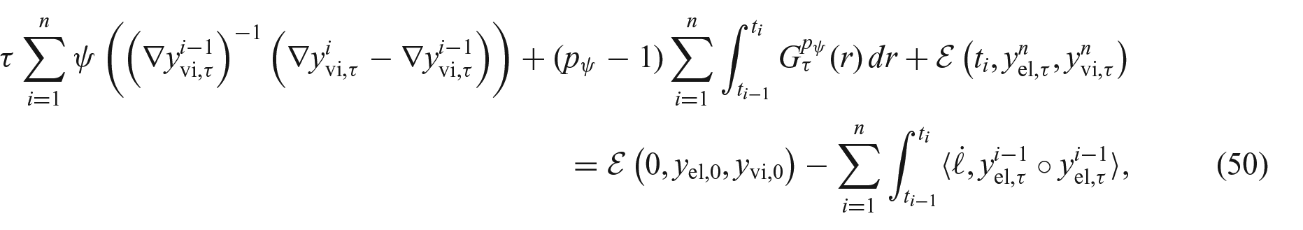
Proposition 6.1. (Discrete energy equality) Let $(y_{\mathrm{el},\tau }^i,y_{\mathrm{vi},\tau }^i{)}_{i=0}^N$ be an incremental solution of the problem of equation (22). Then, for every $1\le n\le N$ , we have:

$$\begin{array}{c}\tau \sum _{i=1}^n\psi \left({(\nabla y_{\mathrm{vi},\tau }^{i-1})}^{-1}(\nabla y_{\mathrm{vi},\tau }^i-\nabla y_{\mathrm{vi},\tau }^{i-1})\right)+(p_{\psi }-1)\sum _{i=1}^n{\int }_{t_{i-1}}^{t_i}{G}_{\tau }^{p_{\psi }}(r)\mathrm{dr}+\mathcal{E}(t_i,y_{\mathrm{el},\tau }^n,y_{\mathrm{vi},\tau }^n)\hfill \\ =\mathcal{E}(0,y_{\mathrm{el},0},y_{\mathrm{vi},0})-\sum _{i=1}^n{\int }_{t_{i-1}}^{t_i}〈\stackrel{·}{\ell },y_{\mathrm{el},\tau }^{i-1}°y_{\mathrm{el},\tau }^{i-1}〉,\hfill \end{array}$$

(50)

where

$$G_{\tau }(t):={({\mathrm{\Psi }}_r^{\pm ,i}(y_{\mathrm{vi},\tau }^{i-1}))}^{1/p_{\psi }}\mathrm{for}t=t_{i-1}+r\in (t_{i-1},t_i].$$

Proof. By equation (49) for $y_{\mathrm{old}}=y_{\mathrm{vi},\tau }^{i-1}$ , $y_{\mathrm{vi},\tau }=y_{\mathrm{vi},\tau }^i$ , and $y_{\mathrm{el},\tau }=y_{\mathrm{el},\tau }^i$ , we find:

$$\begin{array}{c}\tau \mathrm{\Psi }(y_{\mathrm{vi},\tau }^{i-1},\frac{y_{\mathrm{vi},\tau }^i-y_{\mathrm{vi},\tau }^{i-1}}{\tau })+(p_{\psi }-1){\int }_0^{\tau }|G_{\tau }(r){|}^{p_{\psi }}\mathrm{d}r+\mathcal{E}(t_i,y_{\mathrm{el},\tau }^i,y_{\mathrm{vi},\tau }^i)=\mathcal{E}(t_i,y_{\mathrm{el},\tau }^{i-1},y_{\mathrm{vi},\tau }^{i-1})\hfill \\ =\mathcal{E}(t_{i-1},y_{\mathrm{el},\tau }^{i-1},y_{\mathrm{vi},\tau }^{i-1})-{\int }_{t_{i-1}}^{t_i}〈\stackrel{·}{\ell },y_{\mathrm{el},\tau }^{i-1}°y_{\mathrm{el},\tau }^{i-1}〉,\hfill \end{array}$$

where we used the definition of $G_{\tau }$ and of De Giorgi variational interpolation. Then, summing from $i=1$ to $i=n$ , we get equation (50).  □

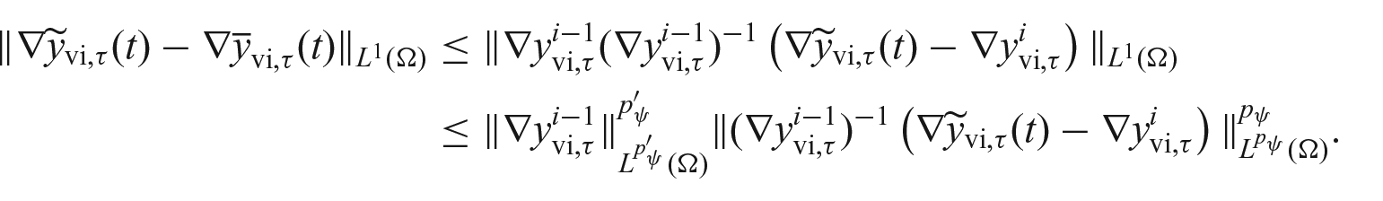
Before passing to the limit for $\tau \to 0$ in the energy equality (50), we need to characterize the limit of the De Giorgi variational interpolation. In the following lemma, we show that such limit coincides with that of the backward interpolants.

Lemma 6.3. If ${\overline{y}}_{\mathrm{vi},\tau }(t)\rightharpoonup y_{\mathrm{vi}}(t)$ in $W^{1,p_{\mathrm{vi}}}(\mathrm{\Omega };{\mathbb{R}}^d)$ , then ${\tilde{y}}_{\mathrm{vi},\tau }(t)\rightharpoonup y_{\mathrm{vi}}(t)$ in $W^{1,p_{\mathrm{vi}}}(\mathrm{\Omega };{\mathbb{R}}^d)$ .

Proof. First, let us show that, for $\tau >0$ and $t\in (t_{i-1}^{\tau },t_i^{\tau }]$ fixed, $\parallel {\tilde{y}}_{\mathrm{vi},\tau }(t)-{\overline{y}}_{\mathrm{vi},\tau }(t){\parallel }_{L^1(\mathrm{\Omega })}\le c{\tau }^{p_{\psi }-1}$ . We have, by definition of $\nabla {\overline{y}}_{\mathrm{vi},\tau }$ and the Hölder inequality:

$$\begin{array}{c}\parallel \nabla {\tilde{y}}_{\mathrm{vi},\tau }(t)-\nabla {\overline{y}}_{\mathrm{vi},\tau }(t){\parallel }_{L^1(\mathrm{\Omega })}\le \parallel \nabla y_{\mathrm{vi},\tau }^{i-1}(\nabla y_{\mathrm{vi},\tau }^{i-1}{)}^{-1}(\nabla {\tilde{y}}_{\mathrm{vi},\tau }(t)-\nabla y_{\mathrm{vi},\tau }^i){\parallel }_{L^1(\mathrm{\Omega })}\hfill \\ \le \parallel \nabla y_{\mathrm{vi},\tau }^{i-1}{\parallel }_{L^{{p_{\psi }}^{\prime }}(\mathrm{\Omega })}^{{p_{\psi }}^{\prime }}\parallel (\nabla y_{\mathrm{vi},\tau }^{i-1}{)}^{-1}(\nabla {\tilde{y}}_{\mathrm{vi},\tau }(t)-\nabla y_{\mathrm{vi},\tau }^i){\parallel }_{L^{p_{\psi }}(\mathrm{\Omega })}^{p_{\psi }}.\hfill \end{array}$$

Since $p_{\psi }\ge 2$ by equation (20), we have that $p_{\psi }^{\prime }\le p_{\psi }$ . Hence, by the boundedness of $\nabla y_{\mathrm{vi},\tau }^{i-1}$ in $L^{p_{\psi }}(\mathrm{\Omega };{\mathbb{R}}^{d\times d})$ and the fact that $\mathrm{\Omega }$ is bounded, we have that $\parallel \nabla y_{\mathrm{vi},\tau }^{i-1}{\parallel }_{L^{{p^{\prime }}_{\psi }}(\mathrm{\Omega })}^{{p^{\prime }}_{\psi }}\le c$ uniformly in $i$ and $\tau$ . Thus, by growth condition (18), we have:

$$\begin{array}{c}\parallel \nabla {\tilde{y}}_{\mathrm{vi},\tau }(t)-\nabla {\overline{y}}_{\mathrm{vi},\tau }(t){\parallel }_{L^1(\mathrm{\Omega })}\le c\parallel (\nabla y_{\mathrm{vi},\tau }^{i-1}{)}^{-1}(\nabla y_{\mathrm{vi},\tau }^i-\nabla y_{\mathrm{vi},\tau }^{i-1}){\parallel }_{L^{p_{\psi }}(\mathrm{\Omega })}^{p_{\psi }}\hfill \\ +c\parallel (\nabla y_{\mathrm{vi},\tau }^{i-1}{)}^{-1}(\nabla {\tilde{y}}_{\mathrm{vi},\tau }(t)-\nabla y_{\mathrm{vi},\tau }^{i-1}){\parallel }_{L^{p_{\psi }}(\mathrm{\Omega })}^{p_{\psi }}\hfill \\ \le c\mathrm{\Psi }(y_{\mathrm{vi},\tau }^{i-1},y_{\mathrm{vi},\tau }^i-y_{\mathrm{vi},\tau }^{i-1})+c\mathrm{\Psi }(y_{\mathrm{vi},\tau }^{i-1},{\tilde{y}}_{\mathrm{vi},\tau }-y_{\mathrm{vi},\tau }^{i-1})\hfill \\ \le c\mathrm{\Psi }(y_{\mathrm{vi},\tau }^{i-1},y_{\mathrm{vi},\tau }^i-y_{\mathrm{vi},\tau }^{i-1}),\hfill \end{array}$$

where in the last inequality, we used the definition of ${\tilde{y}}_{\mathrm{vi},\tau }$ and the monotonicity property (47). Using the $p_{\psi }$ -homogeneity (19) and the boundedness of the dissipation, we get:

$$\parallel \nabla {\tilde{y}}_{\mathrm{vi},\tau }(t)-\nabla {\overline{y}}_{\mathrm{vi},\tau }(t){\parallel }_{L^1(\mathrm{\Omega })}\le c{\tau }^{p_{\psi }}\mathrm{\Psi }(y_{\mathrm{vi},\tau }^{i-1},\frac{y_{\mathrm{vi},\tau }^i-y_{\mathrm{vi},\tau }^{i-1}}{\tau })\le c{\tau }^{p_{\psi }-1}.$$

Then, $\parallel {\tilde{y}}_{\mathrm{vi},\tau }(t)-{\overline{y}}_{\mathrm{vi},\tau }(t){\parallel }_{L^1(\mathrm{\Omega })}\le c{\tau }^{p_{\psi }-1}$ follows since ${\tilde{y}}_{\mathrm{vi},\tau }(t)$ and ${\overline{y}}_{\mathrm{vi},\tau }(t)$ have zero mean.

The assertion follows as $\mathrm{\Omega }$ is bounded, by assumption ${\overline{y}}_{\mathrm{vi},\tau }(t)\rightharpoonup y_{\mathrm{vi}}(t)$ in $W^{1,p_{\mathrm{vi}}}(\mathrm{\Omega };{\mathbb{R}}^d)$ , and ${\overline{y}}_{\mathrm{vi},\tau }(t)$ is bounded in $W^{1,p_{\mathrm{vi}}}(\mathrm{\Omega };{\mathbb{R}}^d)$ by coercivity, as shown in section 6.1 for ${\overline{y}}_{\mathrm{vi},\tau }(t)$ .  □

6.3. Proof of the energy inequality

In the following, we extract further subsequences without relabeling whenever necessary.

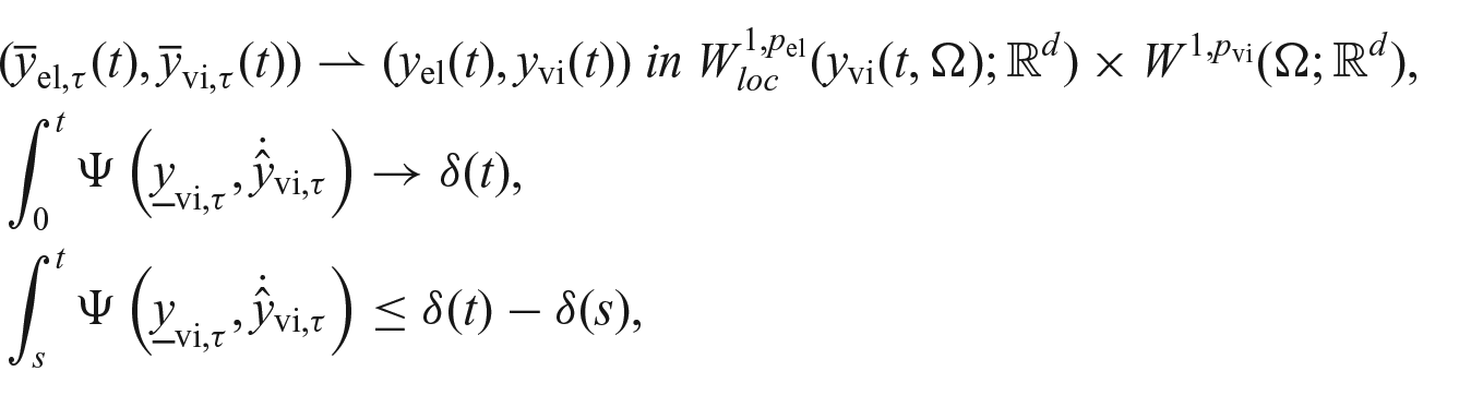
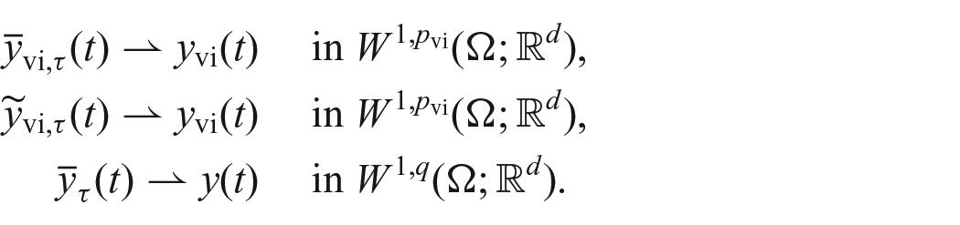
Assume to be given a sequence of partitions $({\mathrm{\Pi }}_{\tau }{)}_{\tau }$ with $\tau \to 0$ and denote by $(y_{\mathrm{el}}^i,y_{\mathrm{vi}}^i{)}_{i=0}^N$ the corresponding incremental solutions. The estimates in section 6.1 and Lemma 6.3 ensure that for every $t\in [0,T]$ :

$$\begin{array}{c}{\overline{y}}_{\mathrm{vi},\tau }(t)\rightharpoonup y_{\mathrm{vi}}(t)\mathrm{in}{W}^{1,p_{\mathrm{vi}}}(\mathrm{\Omega };{\mathbb{R}}^d),\hfill \\ \multicolumn{1}{c}{{\tilde{y}}_{\mathrm{vi},\tau }(t)\rightharpoonup y_{\mathrm{vi}}(t)\mathrm{in}{W}^{1,p_{\mathrm{vi}}}(\mathrm{\Omega };{\mathbb{R}}^d),}\\ \multicolumn{1}{c}{{\overline{y}}_{\tau }(t)\rightharpoonup y(t)\mathrm{in}{W}^{1,q}(\mathrm{\Omega };{\mathbb{R}}^d).}\end{array}$$

Moreover, by Sobolev embedding, we have that ${\hat{y}}_{\mathrm{vi},\tau }\rightharpoonup y_{\mathrm{vi}}$ weakly in $C([0,T];W^{1,p_r}(\mathrm{\Omega };{\mathbb{R}}^d))$ .

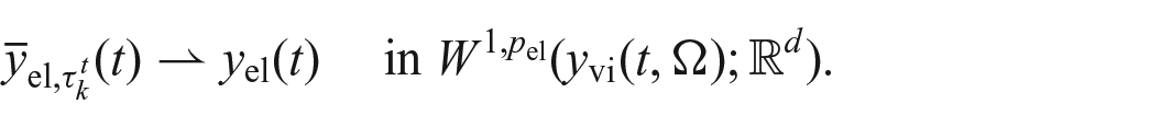
As regards the elastic deformation, given $t\in [0,T]$ by extracting a subsequence $({\tau }_k^t{)}_{k\in \mathbb{N}}$ possibly depending on $t$ , we get:

$${\overline{y}}_{\mathrm{el},{\tau }_k^t}(t)\rightharpoonup y_{\mathrm{el}}(t)\mathrm{in}{W}^{1,p_{\mathrm{el}}}(y_{\mathrm{vi}}(t,\mathrm{\Omega });{\mathbb{R}}^d).$$

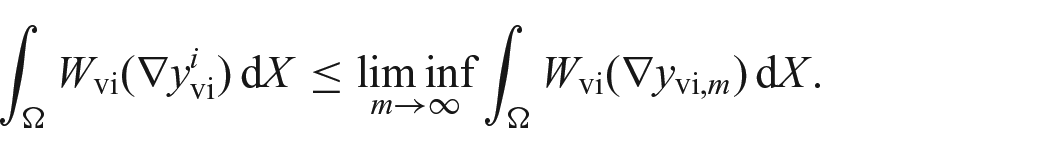
Note that here we have to implement an exhaustion argument for dealing with the moving domains ${\overline{y}}_{\mathrm{vi}}(t,\mathrm{\Omega })$ , exactly as in section 5. Moreover, the total deformation $y$ can be proved to fulfill $y=y_{\mathrm{el}}°y_{\mathrm{vi}}$ by arguing as in section 5.2.

We aim at passing to the limit in the energy equality (50), which can be rewritten, thanks to the definition of $G_{\tau }(t)$ and of ${\mathrm{\Psi }}_r^{+,i}$ , in the weaker form:

$$\begin{array}{c}\mathcal{E}({\overline{t}}_{\tau }(t),{\overline{y}}_{\mathrm{el},\tau }(t),{\overline{y}}_{\mathrm{vi},\tau }(t))+{\int }_0^{{\overline{t}}_{\tau }(t)}\mathrm{\Psi }({\underset{¯}{y}}_{\mathrm{vi},\tau },{\stackrel{·}{\hat{y}}}_{\mathrm{vi},\tau })+(p_{\psi }-1){\int }_0^{{\overline{t}}_{\tau }(t)}\mathrm{\Psi }({\underset{¯}{y}}_{\mathrm{vi},\tau },\frac{{\tilde{y}}_{\mathrm{vi},\tau }-{\underset{¯}{y}}_{\mathrm{vi},\tau }}{\tau })\hfill \\ \le \mathcal{E}(0,y_{\mathrm{el},0},y_{\mathrm{vi},0})-{\int }_0^{{\overline{t}}_{\tau }(t)}〈\stackrel{·}{\ell },{\underset{¯}{y}}_{\tau }〉.\hfill \end{array}$$

(51)

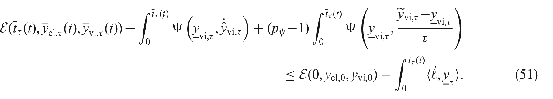
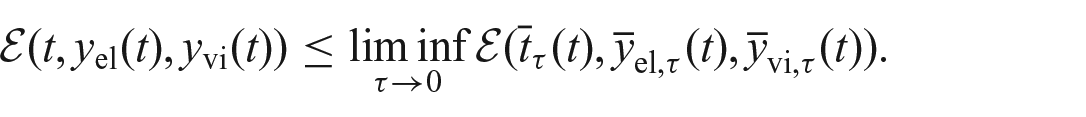
Passing to the $\lim \inf$ in the left-hand side of inequality (51), we find by lower semicontinuity:

$$\mathcal{E}(t,y_{\mathrm{el}}(t),y_{\mathrm{vi}}(t))\le \underset{\tau \to 0}{\lim \inf }\mathcal{E}({\overline{t}}_{\tau }(t),{\overline{y}}_{\mathrm{el},\tau }(t),{\overline{y}}_{\mathrm{vi},\tau }(t)).$$

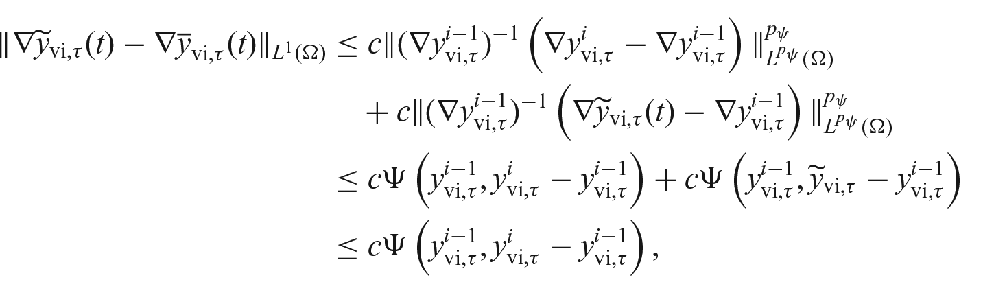
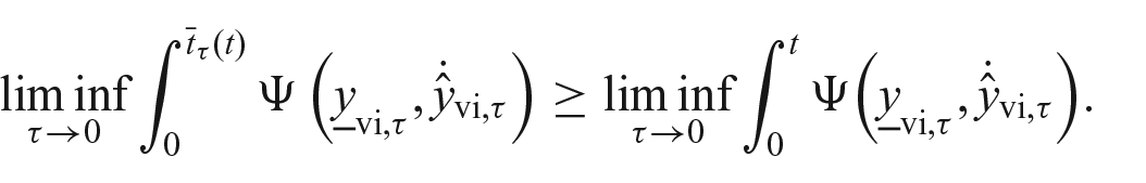
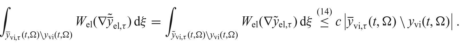
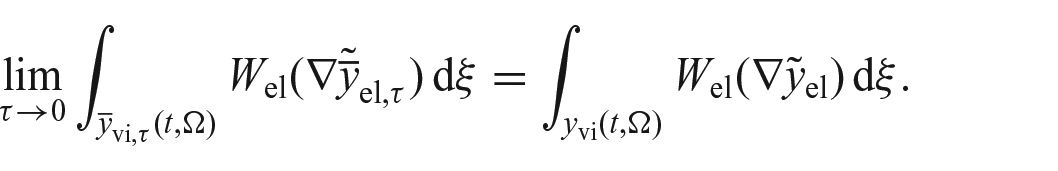
Let us now study the first dissipation term in equation (51). The calculations for the second one are analogous by Lemma 6.3. Recalling that by definition ${\overline{t}}_{\tau }(t)\ge t$ and that $\psi \ge 0$ , we have that:

$$\underset{\tau \to 0}{\lim \inf }{\int }_0^{{\overline{t}}_{\tau }(t)}\mathrm{\Psi }({\underset{¯}{y}}_{\mathrm{vi},\tau },{\stackrel{·}{\hat{y}}}_{\mathrm{vi},\tau })\ge \underset{\tau \to 0}{\lim \inf }{\int }_0^t\mathrm{\Psi }({\underset{¯}{y}}_{\mathrm{vi},\tau },{\stackrel{·}{\hat{y}}}_{\mathrm{vi},\tau }).$$

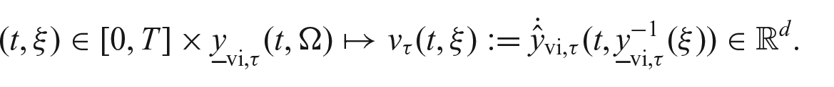
Moreover, up to a subsequence, $\nabla {\stackrel{·}{\hat{y}}}_{\mathrm{vi},\tau }(\nabla {\underset{¯}{y}}_{\mathrm{vi},\tau }{)}^{-1}\rightharpoonup l$ weakly in $L^{p_{\psi }}(\mathrm{\Omega };{\mathbb{R}}^{d\times d})$ by equation (44). It hence remains to identify the limit $l$ . To this end, let us define:

$$(t,\xi )\in [0,T]\times {\underset{¯}{y}}_{\mathrm{vi},\tau }(t,\mathrm{\Omega })\to v_{\tau }(t,\xi ):={\stackrel{·}{\hat{y}}}_{\mathrm{vi},\tau }(t,{\underset{¯}{y}}_{\mathrm{vi},\tau }^{-1}(\xi ))\in {\mathbb{R}}^d.$$

By a pointwise-in-time change of variables, we have:

$${\int }_0^T{\int }_{{\underset{¯}{y}}_{\mathrm{vi},\tau }(t,\mathrm{\Omega })}|v_{\tau }(t,\xi ){|}^{p_{\psi }}\mathrm{d}\xi \mathrm{d}t={\int }_0^T{\int }_{\mathrm{\Omega }}|{\stackrel{·}{\hat{y}}}_{\mathrm{vi},\tau }(t,X){|}^{p_{\psi }}\mathrm{d}X\mathrm{d}t\le c.$$

In order to obtain a bound on the gradient $\nabla v_{\tau }$ , let us consider:

$$\begin{array}{c}{\int }_0^T{\int }_{{\underset{¯}{y}}_{\mathrm{vi},\tau }(t,\mathrm{\Omega })}|\nabla v_{\tau }(t,\xi {)|}^{p_{\psi }}\mathrm{d}\xi \mathrm{d}t={\int }_0^T{\int }_{\mathrm{\Omega }}{|\nabla {\stackrel{·}{\hat{y}}}_{\mathrm{vi},\tau }{(\nabla {\underset{¯}{y}}_{\mathrm{vi},\tau })}^{-1}(t,X)|}^{p_{\psi }}\mathrm{d}X\mathrm{d}t\hfill \\ \multicolumn{1}{c}{\stackrel{(18)}{\le }{\int }_0^T\mathrm{\Psi }({\underset{¯}{y}}_{\mathrm{vi},\tau },{\stackrel{·}{\hat{y}}}_{\mathrm{vi},\tau })\le c.}\end{array}$$

For given $t_0\in (0,T)$ , let us show that ${\cap }_{t\in [t_0,t_0+\delta ]}{y}_{\mathrm{vi}}(t,\mathrm{\Omega })$ is not empty for small $\delta >0$ . Notice that, by Sobolev embedding, ${\underset{¯}{y}}_{\mathrm{vi},\tau }\to y_{\mathrm{vi}}$ in $C([0,T]\times \overline{\mathrm{\Omega }})$ . Hence, for every $ϵ>0$ , there exists $\overline{\tau }=\overline{\tau }(ϵ)$ such that, for every $\tau \le \overline{\tau }$ , we have:

$$\underset{X\in \overline{\mathrm{\Omega }}}{sup}|{\underset{¯}{y}}_{\mathrm{vi},\tau }(t,X)-y_{\mathrm{vi}}(t,X)|\le \frac{ϵ}{2}.$$

Moreover, since $y_{\mathrm{vi}}$ is absolutely continuous in time, for $|t-s|<\nu$ and $\nu >0$ small, we also have:

$$\underset{X\in \overline{\mathrm{\Omega }}}{sup}|y_{\mathrm{vi}}(t,X)-y_{\mathrm{vi}}(s,X)|\le \frac{ϵ}{2}.$$

Combining these two inequalities, we get:

$$\underset{X\in \overline{\mathrm{\Omega }}}{sup}|{\underset{¯}{y}}_{\mathrm{vi},\tau }(t,X)-y_{\mathrm{vi}}(s,X)|\le \epsilon ,$$

for $\tau$ and $\nu$ small enough. We can hence fix $\omega \subset \subset {\cap }_{t\in [t_0,t_0+\nu ]}{\underset{¯}{y}}_{\mathrm{vi}}(t,\mathrm{\Omega })$ and trivially extend $v_{\tau }$ on ${\mathbb{R}}^d\backslash \omega$ .

Then, thanks to the above bounds, we have that $v_{\tau }\rightharpoonup v$ weakly in $L^{p_{\psi }}([0,T];W^{1,p_{\psi }}(\omega ))$ . We have to show that $v={\stackrel{·}{y}}_{\mathrm{vi}}°y_{\mathrm{vi}}^{-1}$ . In fact, we have:

$$\begin{array}{c}{\int }_{t_0}^{t_0+\nu }{\int }_{\omega }v(t,\xi )\mathrm{d}\xi \mathrm{d}t\leftarrow {\int }_{t_0}^{t_0+\nu }{\int }_{\omega }{v}_{\tau }(t,\xi )\mathrm{d}\xi \mathrm{d}t={\int }_{t_0}^{t_0+\nu }{\int }_{{\underset{¯}{y}}_{\mathrm{vi},\tau }^{-1}(t,\omega )}{\stackrel{·}{\hat{y}}}_{\mathrm{vi},\tau }(t,X)\mathrm{d}X\mathrm{d}t\hfill \\ ={\int }_{t_0}^{t_0+\nu }{\int }_{{\mathbb{R}}^d}{\stackrel{·}{\hat{y}}}_{\mathrm{vi},\tau }(t,X)1_{{\underset{¯}{y}}_{\mathrm{vi},\tau }^{-1}(t,\omega )}(t,X)\mathrm{d}X\mathrm{d}t\to {\int }_{t_0}^{t_0+\nu }{\int }_{{\mathbb{R}}^d}{\stackrel{·}{y}}_{\mathrm{vi}}(t,X)1_{y_{\mathrm{vi}}^{-1}(t,\omega )}(t,X)\mathrm{d}X\mathrm{d}t\hfill \\ ={\int }_{t_0}^{t_0+\nu }{\int }_{\omega }{\stackrel{·}{y}}_{\mathrm{vi}}(t,y_{\mathrm{vi}}^{-1}(t,\xi ))\mathrm{d}\xi \mathrm{d}t,\hfill \end{array}$$

(52)

where we have used that ${\hat{y}}_{\mathrm{vi},\tau }\rightharpoonup y_{\mathrm{vi}}$ weakly in $C([0,T];W^{1,p_{\mathrm{vi}}}(\mathrm{\Omega }))$ , $1_{{\underset{¯}{y}}_{\mathrm{vi},\tau }^{-1}(\omega )}\to 1_{y_{\mathrm{vi}}^{-1}(\omega )}$ strongly in $L^1(\omega )$ , and the fact that $1_{{\underset{¯}{y}}_{\mathrm{vi},\tau }^{-1}(t,\omega )}$ is bounded. Since in equation (52) $t_0,\nu ,$ and $\omega$ are arbitrary, we have that $v={\stackrel{·}{y}}_{\mathrm{vi}}°y_{\mathrm{vi}}^{-1}$ and we have hence identified $l=\nabla v$ . By weak lower semicontinuity, we thus have that:

$$\begin{array}{c}\underset{\tau \to 0}{liminf}{\int }_0^{{\overline{t}}_{\tau }(t)}\mathrm{\Psi }({\underset{¯}{y}}_{\mathrm{vi},\tau },{\stackrel{·}{\hat{y}}}_{\mathrm{vi},\tau })=\underset{\tau \to 0}{liminf}{\int }_0^{{\overline{t}}_{\tau }(t)}{\int }_{{\overline{y}}_{\mathrm{vi},\tau }(s,\mathrm{\Omega })}\psi (\nabla v_{\tau }(s,\xi ))\mathrm{d}\xi \mathrm{d}s\hfill \\ \multicolumn{1}{c}{\ge {\int }_0^t{\int }_{y_{\mathrm{vi}}(s,\mathrm{\Omega })}\psi (\nabla v(s,\xi ))\mathrm{d}\xi \mathrm{d}s={\int }_0^t\mathrm{\Psi }(y_{\mathrm{vi},\tau },{\stackrel{·}{y}}_{\mathrm{vi},\tau }).}\end{array}$$

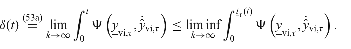
Thanks to the boundedness and to the weak lower semicontinuity of the energy and of the dissipation, we can apply Helly’s Selection Principle [28, Theorem B.5.13, p. 611] and find a nondecreasing function $\delta :[0,T]\to [0,\infty )$ such that:

$${\int }_0^t\mathrm{\Psi }({\underset{¯}{y}}_{\mathrm{vi},\tau },{\stackrel{·}{\hat{y}}}_{\mathrm{vi},\tau })\to \delta (t),$$

(53a)

$${\int }_s^t\mathrm{\Psi }({\underset{¯}{y}}_{\mathrm{vi},\tau },{\stackrel{·}{\hat{y}}}_{\mathrm{vi},\tau })\le \delta (t)-\delta (s),$$

(53b)

for every $s,t\in [0,T]$ . Then, fixing $t\in [0,T]$ , we have:

$$\delta (t)\stackrel{(53)}{=}\underset{k\to \infty }{\lim }{\int }_0^t\mathrm{\Psi }({\underset{¯}{y}}_{\mathrm{vi},\tau },{\stackrel{·}{\hat{y}}}_{\mathrm{vi},\tau })\le \underset{k\to \infty }{liminf}{\int }_0^{{\underset{¯}{t}}_{\tau }(t)}\mathrm{\Psi }({\underset{¯}{y}}_{\mathrm{vi},\tau },{\stackrel{·}{\hat{y}}}_{\mathrm{vi},\tau }).$$

Setting ${\theta }_{\tau }(s):=-〈\stackrel{·}{\ell }(s),{\underset{¯}{y}}_{\tau }(s)〉$ , by the regularity of $\ell$ and the boundedness of $({\underset{¯}{y}}_{\tau }(t){)}_{\tau }$ for almost every $t\in [0,T]$ in $W^{1,q}(\mathrm{\Omega };{\mathbb{R}}^d)$ , we have that $({\theta }_{\tau }{)}_{\tau }$ is equi-integrable. Hence, we can apply the Dunford–Pettis theorem (see, e.g., [28, Theorem B.3.8, p. 598]) to find a subsequence such that:

$${\theta }_{\tau }\rightharpoonup \theta \mathrm{in}{L}^1(0,T).$$

Furthermore, thanks to the boundedness of the energy and the dissipation, we are able to find further $t$ -dependent subsequences $({\tau }_k^t{)}_{k\in \mathbb{N}}$ such that:

$${\theta }_{{\tau }_k^t}\to \underset{\tau \to 0}{\lim \sup }{\theta }_{\tau }(t)=:\overline{\theta }(t),$$

and, by regularity of $\ell$ , that:

$$\overline{\theta }(t):=\underset{k\to \infty }{\lim }{\theta }_{{\tau }_k^t}=\underset{k\to \infty }{\lim }〈\stackrel{·}{\ell }(t),{\underset{¯}{y}}_{{\tau }_k^t}(t)〉=〈\stackrel{·}{\ell }(t),y(t)〉.$$

In conclusion, passing to the $\lim \inf$ in the left-hand side and to the limit in the right-hand side of equation (51), we retrieve energy inequality (23).

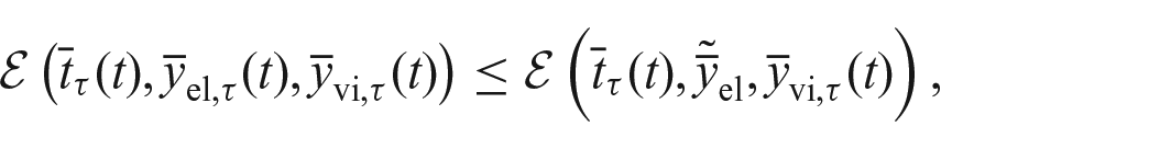
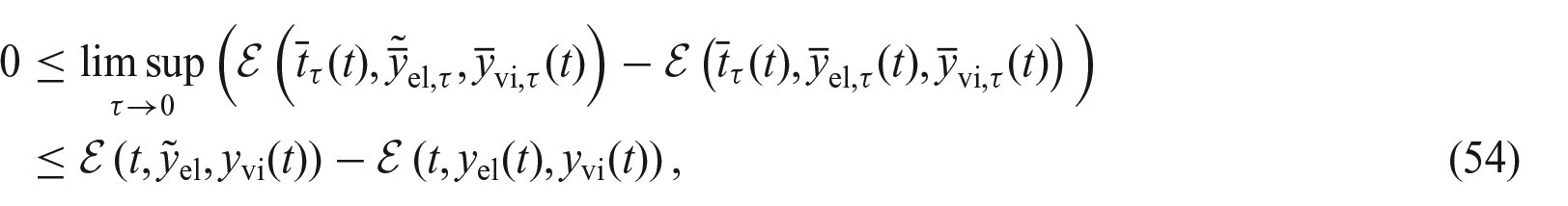
6.4. Proof of the semistability condition

Fix now $t\in [0,T]$ and recall that ${\overline{y}}_{\mathrm{el},{\tau }_k^t}(t)\rightharpoonup y_{\mathrm{el}}(t)$ in $W^{1,p_{\mathrm{el}}}(y_{\mathrm{vi}}(t,\mathrm{\Omega });{\mathbb{R}}^d)$ .

By minimality of the incremental solution, we have:

$$\mathcal{E}({\overline{t}}_{\tau }(t),{\overline{y}}_{\mathrm{el},\tau }(t),{\overline{y}}_{\mathrm{vi},\tau }(t))\le \mathcal{E}({\overline{t}}_{\tau }(t),{\overline{y}}_{\mathrm{el}},{\overline{y}}_{\mathrm{vi},\tau }(t)),$$

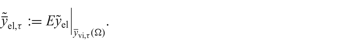
for every ${\overline{y}}_{\mathrm{el}}$ with $({\overline{y}}_{\mathrm{el}},{\overline{y}}_{\mathrm{vi}}(t))\in \mathcal{A}$ . Let $({\tilde{y}}_{\mathrm{el}},y_{\mathrm{vi}}(t))\in \mathcal{A}$ be given. We want to show that one can choose ${\overline{y}}_{\mathrm{el},\tau }$ with $({\overline{y}}_{\mathrm{el},\tau },{\overline{y}}_{\mathrm{vi}}(t))\in \mathcal{A}$ in such a way that:

$$\begin{array}{c}0\le \underset{\tau \to 0}{\lim \sup }(\mathcal{E}({\overline{t}}_{\tau }(t),{\overline{y}}_{\mathrm{el},\tau },{\overline{y}}_{\mathrm{vi},\tau }(t))-\mathcal{E}({\overline{t}}_{\tau }(t),{\overline{y}}_{\mathrm{el},\tau }(t),{\overline{y}}_{\mathrm{vi},\tau }(t)))\hfill \\ \le \mathcal{E}(t,{\tilde{y}}_{\mathrm{el}},y_{\mathrm{vi}}(t))-\mathcal{E}(t,y_{\mathrm{el}}(t),y_{\mathrm{vi}}(t)),\hfill \end{array}$$

(54)

which would then imply equation (24).

Since $({\tilde{y}}_{\mathrm{el}},y_{\mathrm{vi}}(t))\in \mathcal{A}$ , we have that $y_{\mathrm{vi}}(\mathrm{\Omega })\in {\mathcal{J}}_{{\eta }_1,{\eta }_2}$ and $y_{\mathrm{vi}}(\mathrm{\Omega })$ is a Sobolev extension domain. Hence, there exists a linear and bounded extension operator $E:W^{1,p_{\mathrm{el}}}(y_{\mathrm{vi}}(\mathrm{\Omega });{\mathbb{R}}^d)$ → $W^{1,p_{\mathrm{el}}}({\mathbb{R}}^d;{\mathbb{R}}^d)$ . We thus define ${\overline{y}}_{\mathrm{el},\tau }\in W^{1,p_{\mathrm{el}}}({\overline{y}}_{\mathrm{vi},\tau }(\mathrm{\Omega });{\mathbb{R}}^d)$ as the restriction to ${\overline{y}}_{\mathrm{vi},\tau }(\mathrm{\Omega })$ of the extension $E{\tilde{y}}_{\mathrm{el}}$ , namely,

$${\overline{y}}_{\mathrm{el},\tau }:=E{\tilde{y}}_{\mathrm{el}}{|}_{{\overline{y}}_{\mathrm{vi},\tau }(\mathrm{\Omega })}.$$

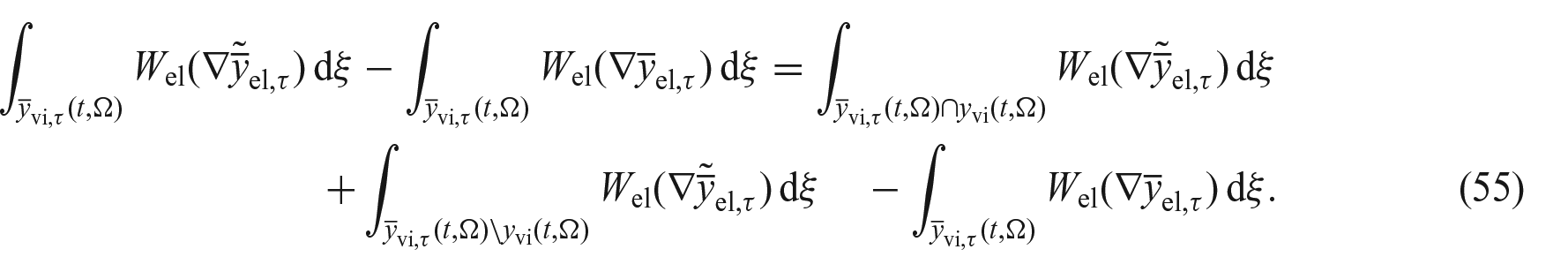
In the following, we just concentrate our attention on the stored elastic energy part, since the treatment of the loading term is immediate. We write:

$$\begin{array}{c}{\int }_{{\overline{y}}_{\mathrm{vi},\tau }(t,\mathrm{\Omega })}{W}_{\mathrm{el}}(\nabla {\overline{y}}_{\mathrm{el},\tau })\mathrm{d}\xi -{\int }_{{\overline{y}}_{\mathrm{vi},\tau }(t,\mathrm{\Omega })}{W}_{\mathrm{el}}(\nabla {\overline{y}}_{\mathrm{el},\tau })\mathrm{d}\xi ={\int }_{{\overline{y}}_{\mathrm{vi},\tau }(t,\mathrm{\Omega })\cap y_{\mathrm{vi}}(t,\mathrm{\Omega })}{W}_{\mathrm{el}}(\nabla {\overline{y}}_{\mathrm{el},\tau })\mathrm{d}\xi \hfill \\ +{\int }_{{\overline{y}}_{\mathrm{vi},\tau }(t,\mathrm{\Omega })\backslash y_{\mathrm{vi}}(t,\mathrm{\Omega })}{W}_{\mathrm{el}}(\nabla {\overline{y}}_{\mathrm{el},\tau })\mathrm{d}\xi -{\int }_{{\overline{y}}_{\mathrm{vi},\tau }(t,\mathrm{\Omega })}{W}_{\mathrm{el}}(\nabla {\overline{y}}_{\mathrm{el},\tau })\mathrm{d}\xi .\hfill \end{array}$$

(55)

By the growth condition (14) on $W_{\mathrm{el}}$ and the fact that on the set ${\overline{y}}_{\mathrm{vi},\tau }(t,\mathrm{\Omega })$ we have ${\overline{y}}_{\mathrm{el},\tau }={\tilde{y}}_{\mathrm{el},\tau }$ , which is uniformly bounded in $W^{1,p_{\mathrm{el}}}(y_{\mathrm{vi},\tau }(t,\mathrm{\Omega });{\mathbb{R}}^d)$ , we find:

$${\int }_{{\overline{y}}_{\mathrm{vi},\tau }(t,\mathrm{\Omega })\backslash y_{\mathrm{vi}}(t,\mathrm{\Omega })}{W}_{\mathrm{el}}(\nabla {\overline{y}}_{\mathrm{el},\tau })\mathrm{d}\xi ={\int }_{{\tilde{y}}_{\mathrm{vi},\tau }(t,\mathrm{\Omega })\backslash y_{\mathrm{vi}}(t,\mathrm{\Omega })}{W}_{\mathrm{el}}(\nabla {\tilde{y}}_{\mathrm{el},\tau })\mathrm{d}\xi \stackrel{(14)}{\le }c|{\overline{y}}_{\mathrm{vi},\tau }(t,\mathrm{\Omega })\backslash y_{\mathrm{vi}}(t,\mathrm{\Omega })|.$$

Since the measure of the set ${\overline{y}}_{\mathrm{vi},\tau }(t,\mathrm{\Omega })\backslash y_{\mathrm{vi}}(t,\mathrm{\Omega })$ vanishes as $\tau$ goes to $0$ by the uniform convergence of ${\overline{y}}_{\mathrm{vi},\tau }$ to $y_{\mathrm{vi}}$ , we have:

$$\underset{\tau \to 0}{\lim }{\int }_{{\overline{y}}_{\mathrm{vi},\tau }(t,\mathrm{\Omega })}{W}_{\mathrm{el}}(\nabla {\overline{y}}_{\mathrm{el},\tau })d\xi ={\int }_{y_{\mathrm{vi}}(t,\mathrm{\Omega })}{W}_{\mathrm{el}}(\nabla {\tilde{y}}_{\mathrm{el}})d\xi .$$

We can hence pass to the $\lim \sup$ in inequality (55) as $\tau \to 0$ and obtain equation (54), which is nothing but the semistability (24).

7. Linearization: Proof of Theorem 4.2

We first prove in section 7.1 some coercivity results, uniform with respect to the linearization parameter $\epsilon$ , which in turn provide a priori estimates on the sequence of approximable solutions $(u_{\epsilon },v_{\epsilon }{)}_{\epsilon }$ . Then, we check in section 7.2 some $\mathrm{\Gamma }$ - $\lim \inf$ inequalities for the energy and the dissipation. Eventually, in section 7.3, we show that the approximable solutions $(u_{\epsilon },v_{\epsilon }{)}_{\epsilon }$ converge, up to subsequences, to solutions of the linearized problem in the sense of Theorem 4.2.

In the following, we use the notation:

$$W_{\mathrm{el}}^{\epsilon }(A):=\frac{1}{{\epsilon }^2}{W}_{\mathrm{el}}(I+\epsilon A),{\tilde{W}}_{\mathrm{vi}}^{\epsilon }(A):=\frac{1}{{\epsilon }^2}{\tilde{W}}_{\mathrm{vi}}(I+\epsilon A),{\psi }^{\epsilon }(A):=\frac{1}{{\epsilon }^2}\psi (\epsilon A),$$

for the rescaled energy and dissipation densities.

7.1. Coercivity

We devote this section to the proof of the following.

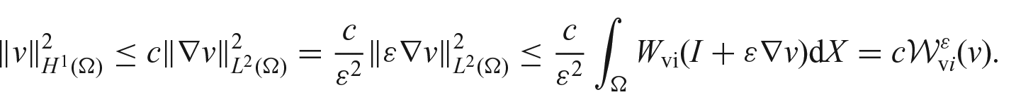
Lemma 7.1. (Coercivity) For every $(u,v)\in {\tilde{\mathcal{A}}}_{\epsilon }$ , it holds:

$$\parallel u{\parallel }_{H^1(\mathrm{\Omega })}^2+\parallel v{\parallel }_{H^1(\mathrm{\Omega })}^2+\parallel \nabla \stackrel{·}{v}{\parallel }_{L^2(\mathrm{\Omega })}^2+\parallel \epsilon \nabla v{\parallel }_{L^{\infty }(\mathrm{\Omega })}\le c(1+{\mathcal{W}}_{\mathrm{vi}}^{\epsilon }(v)+{\mathcal{W}}_{\mathrm{el}}^{\epsilon }(u,v)+{\mathrm{\Psi }}^{\epsilon }(v)).$$

Notice the bound on the term $\parallel \epsilon \nabla v{\parallel }_{L^{\infty }(\mathrm{\Omega })}$ , which follows from assumption (L4). This bound will play an important role in passing to the limit for $\epsilon \to 0$ .

Proof of Lemma 7.1. With no loss of generality, we can assume ${\mathcal{W}}_{\mathrm{vi}}^{\epsilon }(v)+{\mathcal{W}}_{\mathrm{el}}^{\epsilon }(u,v)+{\mathrm{\Psi }}^{\epsilon }(v)<\infty$

By assumption (L4), we have that $I+\epsilon \nabla v\in K\subset \subset \mathrm{SL}(d)$ almost everywhere in $\mathrm{\Omega }$ . Using equation (31), we get that $|I+\epsilon \nabla v|\le c_K$ , hence:

$$\parallel \epsilon \nabla v{\parallel }_{L^{\infty }(\mathrm{\Omega })}\le c.$$

Since $v$ has zero mean by assumption, by applying the Poincaré–Wirtinger inequality and by taking into account the growth condition (29), we get:

$$\parallel v{\parallel }_{H^1(\mathrm{\Omega })}^2\le c\parallel \nabla v{\parallel }_{L^2(\mathrm{\Omega })}^2=\frac{c}{{\epsilon }^2}\parallel \epsilon \nabla v{\parallel }_{L^2(\mathrm{\Omega })}^2\le \frac{c}{{\epsilon }^2}{\int }_{\mathrm{\Omega }}{W}_{\mathrm{vi}}(I+\epsilon \nabla v)\mathrm{dX}=c{\mathcal{W}}_{\mathrm{vi}}^{\epsilon }(v).$$

Using condition (32) and the fact that $|I+\epsilon \nabla v|$ is bounded in $L^{\infty }$ , we get:

$$\begin{array}{c}\parallel \nabla \stackrel{·}{v}{\parallel }_{L^2(\mathrm{\Omega })}^2=\frac{1}{{\epsilon }^2}{\int }_{\mathrm{\Omega }}|\epsilon \nabla \stackrel{·}{v}{|}^2\mathrm{d}X\le \frac{1}{{\epsilon }^2}{\int }_{\mathrm{\Omega }}|\epsilon \nabla \stackrel{·}{v}{|}^2|I+\epsilon \nabla v{|}^{-2}|I+\epsilon \nabla v{|}^2\mathrm{d}X\hfill \\ \multicolumn{1}{c}{\le \frac{c}{{\epsilon }^2}{\int }_{\mathrm{\Omega }}\psi (\epsilon \nabla \stackrel{·}{v}{(I+\epsilon \nabla v)}^{-1})\mathrm{d}X=c{\mathrm{\Psi }}^{\epsilon }(v).}\end{array}$$

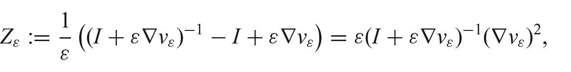
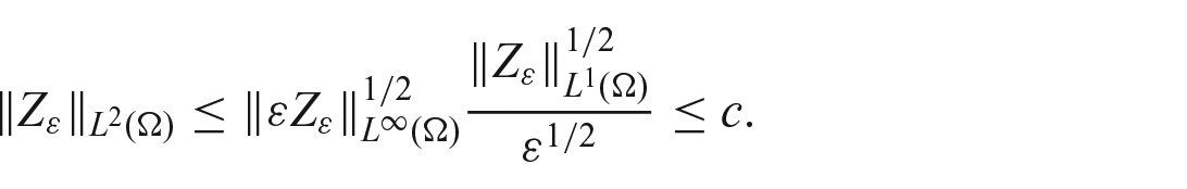
In order to obtain the $H^1$ -bound on $u$ , we start by fixing $Q\in \mathrm{SO}(d)$ and define $F_{\mathrm{el}}:=\nabla y(I+\epsilon \nabla v{)}^{-1}$ , where we recall that $y=\mathrm{id}+\epsilon u$ . We have:

$$\begin{array}{c}|\nabla y-Q{|}^2=|\nabla y-Q(I+\epsilon \nabla v)+\epsilon Q\nabla v{|}^2=|(F_{\mathrm{el}}-Q)(I+\epsilon \nabla v)+\epsilon Q\nabla v{|}^2\hfill \\ \multicolumn{1}{c}{\le c(|F_{\mathrm{el}}-Q{|}^2|I+\epsilon \nabla v{|}^2+{\epsilon }^2|\nabla v{|}^2)\le c(|F_{\mathrm{el}}-Q{|}^2+{\epsilon }^2|\nabla v{|}^2).}\end{array}$$

Taking the infimum over $Q\in \mathrm{SO}(d)$ , we get:

$$\mathrm{dis}{\mathrm{t}}^2(\nabla y,\mathrm{SO}(d))\le c(\mathrm{dis}{\mathrm{t}}^2(F_{\mathrm{el}},\mathrm{SO}(d))+{\epsilon }^2|\nabla v{|}^2).$$

We now integrate over $\mathrm{\Omega }$ and, thanks to assumption (26) and the estimate on $\parallel v{\parallel }_{H^1(\mathrm{\Omega })}^2$ , we find:

$${\int }_{\mathrm{\Omega }}\mathrm{dis}{\mathrm{t}}^2(\nabla y,\mathrm{SO}(d))\mathrm{dX}\le c{\int }_{\mathrm{\Omega }}{W}_{\mathrm{el}}(F_{\mathrm{el}})\mathrm{dX}+c{\epsilon }^2\parallel \nabla v{\parallel }_{L^2(\mathrm{\Omega })}^2\le c{\epsilon }^2({\mathcal{W}}_{\mathrm{el}}^{\epsilon }(u,v)+{\mathcal{W}}_{\mathrm{vi}}^{\epsilon }(v)).$$

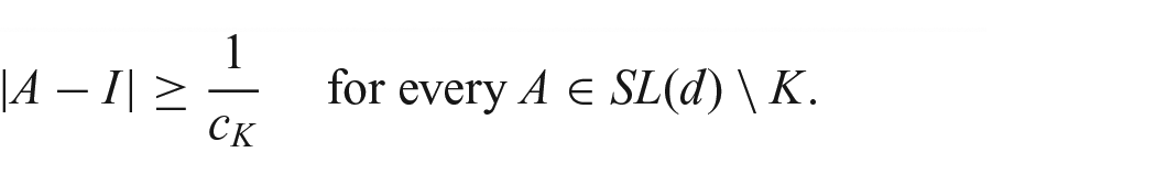
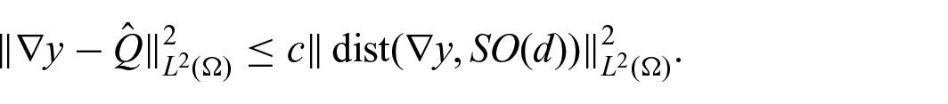
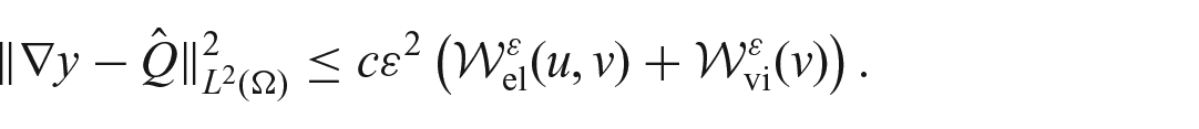
The classical Rigidity Estimate [45, Theorem 3.1] implies that there exists a constant rotation $\hat{Q}\in \mathrm{SO}(d)$ such that:

$$\parallel \nabla y-\hat{Q}{\parallel }_{L^2(\mathrm{\Omega })}^2\le c\parallel \mathrm{dist}(\nabla y,\mathrm{SO}(d)){\parallel }_{L^2(\mathrm{\Omega })}^2.$$

We hence have that:

$$\parallel \nabla y-\hat{Q}{\parallel }_{L^2(\mathrm{\Omega })}^2\le c{\epsilon }^2({\mathcal{W}}_{\mathrm{el}}^{\epsilon }(u,v)+{\mathcal{W}}_{\mathrm{vi}}^{\epsilon }(v)).$$

Recalling that $y=\mathrm{id}$ on ${\mathrm{\Gamma }}_D$ , by Maso et al. [32], (3.14), we also deduce:

$$\parallel I-\hat{Q}{\parallel }_{L^2(\mathrm{\Omega })}^2\le c{\epsilon }^2({\mathcal{W}}_{\mathrm{el}}^{\epsilon }(u,v)+{\mathcal{W}}_{\mathrm{vi}}^{\epsilon }(v)).$$

In conclusion, we get that:

$$\begin{array}{c}\parallel \nabla u{\parallel }_{L^2(\mathrm{\Omega })}^2=\frac{1}{{\epsilon }^2}\parallel \nabla y-I{\parallel }_{L^2(\mathrm{\Omega })}^2\le \frac{2}{{\epsilon }^2}\parallel \nabla y-\hat{Q}{\parallel }_{L^2(\mathrm{\Omega })}^2+\frac{2}{{\epsilon }^2}\parallel \hat{Q}-I{\parallel }_{L^2(\mathrm{\Omega })}^2\hfill \\ \le c({\mathcal{W}}_{\mathrm{el}}^{\epsilon }(u,v)+{\mathcal{W}}_{\mathrm{vi}}^{\epsilon }(v)),\hfill \end{array}$$

whence the assertion follows.  □

7.2. $\mathrm{\Gamma }$ - $\lim \inf$ inequalities

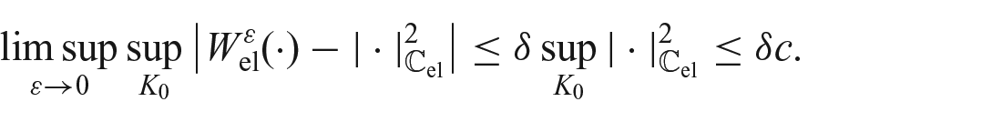
In order to proceed with the linearization, we need to establish $\mathrm{\Gamma }$ - $\lim \inf$ inequalities. At first, we prove the following lemma on the convergence of the densities.

Lemma 7.2. (Convergence of the densities) Assume conditions (L3), (L6), and (L9). Then, we have:

$$W_{\mathrm{el}}^{\epsilon }\to |·{|}_{{\mathbb{C}}_{\mathrm{el}}}^2,{\tilde{W}}_{\mathrm{vi}}^{\epsilon }\to |·{|}_{{\mathbb{C}}_{\mathrm{vi}}}^2,{\psi }^{\epsilon }\to |·{|}_{\mathbb{D}}^2,$$

locally uniformly. Moreover, we have:

$$|z{|}_{{\mathbb{C}}_{\mathrm{el}}}^2\le inf\{\underset{\epsilon \to 0}{\lim \inf }{W}_{\mathrm{el}}^{\epsilon }(z_{\epsilon })|z_{\epsilon }\to z\mathrm{in}{\mathbb{R}}^{d\times d}\},$$

(56)

$$|z{|}_{{\mathbb{C}}_{\mathrm{vi}}}^2\le inf\{\underset{\epsilon \to 0}{\lim \inf }{\tilde{W}}_{\mathrm{vi}}^{\epsilon }(z_{\epsilon })|z_{\epsilon }\to z\mathrm{in}{\mathbb{R}}^{d\times d}\},$$

(57)

$$|z{|}_{\mathbb{D}}^2\le inf\{\underset{\epsilon \to 0}{\lim \inf }{\psi }^{\epsilon }(z_{\epsilon })|z_{\epsilon }\to z\mathrm{in}{\mathbb{R}}^{d\times d}\}.$$

(58)

Proof. Let $K_0\subset \subset {\mathbb{R}}^{d\times d}$ be given. Fix $\delta >0$ and let $c_{\mathrm{el}}(\delta )$ be the corresponding constant from assumption (28). Then, for sufficiently small $\epsilon$ , we have that $\epsilon K_0\subset B_{c_{\mathrm{el}}(\delta )}(0)$ . Hence, by equation (28), we find:

$$\underset{\epsilon \to 0}{\lim \sup }\underset{K_0}{sup}|W_{\mathrm{el}}^{\epsilon }(·)-|·{|}_{{\mathbb{C}}_{\mathrm{el}}}^2|\le \delta \underset{K_0}{sup}|·{|}_{{\mathbb{C}}_{\mathrm{el}}}^2\le \delta c.$$

Since $\delta$ is arbitrary, we get local uniform convergence for $W_{\mathrm{el}}^{\epsilon }$ . For ${\tilde{W}}_{\mathrm{vi}}^{\epsilon }$ and ${\psi }^{\epsilon }$ , proof of convergence is analogous, using the corresponding conditions (30) and (33), respectively.

For the $\mathrm{\Gamma }$ - $\lim \inf$ inequalities (56)–(58), let $(z_{\epsilon }{)}_{\epsilon }\subset {\mathbb{R}}^{d\times d}$ be such that $z_{\epsilon }\to z$ in ${\mathbb{R}}^{d\times d}$ . Assume without loss of generality that $\underset{\epsilon }{sup}{W}_{\mathrm{el}}^{\epsilon }(z_{\epsilon })<\infty .$ Then, the inequality follows from local uniform convergence. The same applies to ${\tilde{W}}_{\mathrm{vi}}^{\epsilon }$ and ${\psi }^{\epsilon }$ . □

We are now in the position of proving the $\mathrm{\Gamma }$ - $\lim \inf$ inequalities for the functionals.

Lemma 7.3. ( $\mathrm{\Gamma }$ - $\lim \inf$ inequalities) For every $(u,v)\in {\tilde{\mathcal{A}}}_{\epsilon }$ , we have:

$$\begin{array}{c}{\mathcal{W}}_{\mathrm{el}}^0(u,v)+{\mathcal{W}}_{\mathrm{vi}}^0(v)\le inf\{\underset{\epsilon \to 0}{\lim \inf }({\mathcal{W}}_{\mathrm{el}}^{\epsilon }(u_{\epsilon },v_{\epsilon })+{\mathcal{W}}_{\mathrm{vi}}^{\epsilon }(v_{\epsilon }))\hfill \\ \multicolumn{1}{c}{|(u_{\epsilon },v_{\epsilon })\rightharpoonup (u,v)\mathrm{weakly}\mathrm{in}{H}^1{(\mathrm{\Omega };{\mathbb{R}}^d)}^2\},}\end{array}$$

$${\int }_0^t{\mathrm{\Psi }}^0(\stackrel{·}{v})\le inf\{\underset{\epsilon \to 0}{\lim \inf }{\int }_0^t{\mathrm{\Psi }}^{\epsilon }(v_{\epsilon },{\stackrel{·}{v}}_{\epsilon })|v_{\epsilon }\rightharpoonup v\mathrm{weakly}\mathrm{in}{H}^1([0,t];L^2(\mathrm{\Omega };{\mathbb{R}}^d))\}.$$

Proof. Let $(u_{\epsilon },v_{\epsilon })\rightharpoonup (u,v)\mathrm{weakly}\mathrm{in}{H}^1(\mathrm{\Omega };{\mathbb{R}}^d{)}^2$ and assume without loss of generality that $\underset{\epsilon }{sup}({\mathcal{W}}_{\mathrm{el}}^{\epsilon }(u_{\epsilon },v_{\epsilon })$ $+{\mathcal{W}}_{\mathrm{vi}}^{\epsilon }(v_{\epsilon }))<\infty$ .

Thanks to inequality (57) and [15, Lemma 4.2], we immediately handle the stored viscous energy terms as:

$${\int }_{\mathrm{\Omega }}|\nabla v{|}_{{\mathbb{C}}_{\mathrm{vi}}}^2\mathrm{d}X\le \underset{\epsilon \to 0}{\lim \inf }{\int }_{\mathrm{\Omega }}{W}_{\mathrm{vi}}^{\epsilon }(\nabla v_{\epsilon })\mathrm{d}X=\underset{\epsilon \to 0}{\lim \inf }\frac{1}{{\epsilon }^2}{\int }_{\mathrm{\Omega }}{W}_{\mathrm{vi}}(I+\epsilon \nabla v_{\epsilon })\mathrm{d}X.$$

The treatment of the stored elastic energy term requires some steps. First, notice that, since $\underset{\epsilon }{sup}{\mathcal{W}}_{\mathrm{vi}}^{\epsilon }(v_{\epsilon })<\infty$ , we have that $I+\epsilon \nabla v_{\epsilon }\in K$ almost everywhere in $\mathrm{\Omega }$ . Hence, $\parallel \epsilon \nabla v_{\epsilon }{\parallel }_{L^{\infty }(\mathrm{\Omega })}\le c$ uniformly in $\epsilon$ and $(I+\epsilon \nabla v_{\epsilon }{)}^{-1}$ is bounded in $L^{\infty }(\mathrm{\Omega };{\mathbb{R}}^{d\times d})$ by equation (31) as well.

Let us then define the auxiliary tensor $Z_{\epsilon }$ as:

$$Z_{\epsilon }:=\frac{1}{\epsilon }({(I+\epsilon \nabla v_{\epsilon })}^{-1}-I+\epsilon \nabla v_{\epsilon })=\epsilon (I+\epsilon \nabla v_{\epsilon }{)}^{-1}(\nabla v_{\epsilon }{)}^2,$$

so that $(I+\epsilon \nabla v_{\epsilon }{)}^{-1}=I-\epsilon \nabla v_{\epsilon }+\epsilon Z_{\epsilon }$ . Notice that $\parallel \epsilon Z_{\epsilon }{\parallel }_{L^{\infty }(\mathrm{\Omega })}\le c$ since $\parallel \epsilon \nabla v_{\epsilon }{\parallel }_{L^{\infty }(\mathrm{\Omega })}\le c$ .

Furthermore,

$$\parallel Z_{\epsilon }{\parallel }_{L^1(\mathrm{\Omega })}\le \epsilon \parallel (I+\epsilon \nabla v_{\epsilon }{)}^{-1}(\nabla v_{\epsilon }{)}^2{\parallel }_{L^1(\mathrm{\Omega })}\le c\epsilon \parallel \nabla v_{\epsilon }{\parallel }_{L^2(\mathrm{\Omega })}\le c\epsilon .$$

Hence, $Z_{\epsilon }$ is bounded in $L^2(\mathrm{\Omega };{\mathbb{R}}^{d\times d})$ by interpolation, namely,

$$\parallel Z_{\epsilon }{\parallel }_{L^2(\mathrm{\Omega })}\le \parallel \epsilon Z_{\epsilon }{\parallel }_{L^{\infty }(\mathrm{\Omega })}^{1/2}\frac{\parallel Z_{\epsilon }{\parallel }_{L^1(\mathrm{\Omega })}^{1/2}}{{\epsilon }^{1/2}}\le c.$$

We therefore conclude that $Z_{\epsilon }\rightharpoonup 0$ weakly in $L^2(\mathrm{\Omega };{\mathbb{R}}^{d\times d})$ .

Define now $F_{\mathrm{el}}^{\epsilon }:=(I+\epsilon \nabla u_{\epsilon })(I+\epsilon \nabla v_{\epsilon }{)}^{-1}$ and

$$A^{\epsilon }:=\frac{F_{\mathrm{el}}^{\epsilon }-I}{\epsilon }=\frac{1}{\epsilon }((I+\epsilon \nabla u_{\epsilon })(I+\epsilon \nabla v_{\epsilon }{)}^{-1}-I).$$

We want to show that $A^{\epsilon }\rightharpoonup \nabla u-\nabla v$ weakly in $L^2(\mathrm{\Omega };{\mathbb{R}}^{d\times d})$ . Let us compute:

$$A^{\epsilon }=\frac{1}{\epsilon }((I+\epsilon \nabla u_{\epsilon })(I-\epsilon \nabla v_{\epsilon }+\epsilon Z_{\epsilon })-I)=\nabla u_{\epsilon }-\nabla v_{\epsilon }+Z_{\epsilon }-\epsilon (\nabla u_{\epsilon }\nabla v_{\epsilon }-\nabla u_{\epsilon }{Z}_{\epsilon }).$$

Since $\nabla u_{\epsilon }-\nabla v_{\epsilon }\rightharpoonup \nabla u-\nabla v$ and $Z_{\epsilon }\rightharpoonup 0$ weakly in $L^2(\mathrm{\Omega };{\mathbb{R}}^{d\times d})$ , it remains to show that: $H_{\epsilon }:=\epsilon (\nabla u_{\epsilon }\nabla v_{\epsilon }-\nabla u_{\epsilon }{Z}_{\epsilon })\rightharpoonup 0$ weakly in $L^2(\mathrm{\Omega };{\mathbb{R}}^{d\times d})$ . Notice that $\parallel H_{\epsilon }{\parallel }_{L^2(\mathrm{\Omega })}\le c$ since $\nabla u_{\epsilon }$ is bounded in $L^2(\mathrm{\Omega };{\mathbb{R}}^{d\times d})$ and $\epsilon \nabla v_{\epsilon }$ and $\epsilon Z_{\epsilon }$ are bounded in $L^{\infty }(\mathrm{\Omega };{\mathbb{R}}^{d\times d})$ . Moreover, since $\nabla v_{\epsilon }$ and $Z_{\epsilon }$ are bounded in $L^2(\mathrm{\Omega };{\mathbb{R}}^{d\times d})$ , then $\parallel H_{\epsilon }{\parallel }_{L^1(\mathrm{\Omega })}\le c\epsilon$ so that $H_{\epsilon }\rightharpoonup 0$ weakly in $L^2(\mathrm{\Omega };{\mathbb{R}}^{d\times d})$ .

Hence, we have by equation (56) and [15, Lemma 4.2] that:

$$\begin{array}{c}{\int }_{\mathrm{\Omega }}|\nabla u-\nabla v{|}_{{\mathbb{C}}_{\mathrm{el}}}^2\mathrm{dX}\le \underset{\epsilon \to 0}{\lim \inf }{\int }_{\mathrm{\Omega }}{W}_{\mathrm{el}}^{\epsilon }(A^{\epsilon })\mathrm{dX}\hfill \\ =\underset{\epsilon \to 0}{\lim \inf }\frac{1}{{\epsilon }^2}{\int }_{\mathrm{\Omega }}{W}_{\mathrm{el}}((I+\epsilon \nabla u_{\epsilon })(I+\epsilon \nabla v_{\epsilon }{)}^{-1})\mathrm{dX}.\hfill \end{array}$$

Let $(v_{\epsilon }{)}_{\epsilon }$ be such that $v_{\epsilon }\rightharpoonup v$ weakly in $H^1([0,t];L^2(\mathrm{\Omega };{\mathbb{R}}^d))$ , and $\underset{\epsilon }{sup}{\mathrm{\Psi }}^{\epsilon }(v_{\epsilon },{\stackrel{·}{v}}_{\epsilon })<\infty$ . By coercivity, we have that (up to a nonrelabeled subsequence) $\nabla {\stackrel{·}{v}}_{\epsilon }(I+\epsilon \nabla v_{\epsilon }{)}^{-1}\rightharpoonup Y$ weakly in $L^2(\mathrm{\Omega })$ . We want to identify the limit as $Y=\nabla \stackrel{·}{v}$ . First, notice that:

$$\nabla {\stackrel{·}{v}}_{\epsilon }(I+\epsilon \nabla v_{\epsilon }{)}^{-1}-\nabla {\stackrel{·}{v}}_{\epsilon }=-\epsilon \nabla {\stackrel{·}{v}}_{\epsilon }\nabla v_{\epsilon }(I+\epsilon \nabla v_{\epsilon }{)}^{-1}=:Y_{\epsilon }\rightharpoonup 0\mathrm{weakly}\mathrm{in}{L}^2(\mathrm{\Omega };{\mathbb{R}}^{d\times d}).$$

Indeed, $\parallel Y_{\epsilon }{\parallel }_{L^1(\mathrm{\Omega })}\le c\epsilon$ and $\parallel Y_{\epsilon }{\parallel }_{L^2(\mathrm{\Omega })}\le c$ . Then, the $\mathrm{\Gamma }$ - $\lim \inf$ inequality for the dissipation term follows from equation (58) and Mielke and Stefanelli [15, Lemma 4.2] applied on the domain $[0,t]\times \mathrm{\Omega }$ .  □

7.3. Convergence of approximable solutions

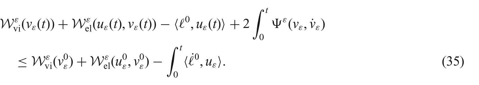
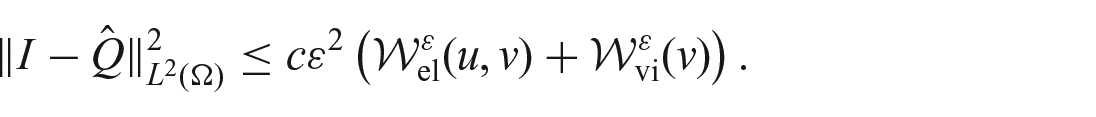
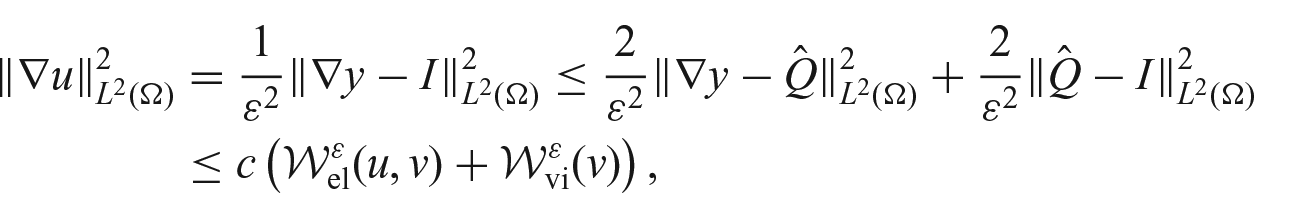
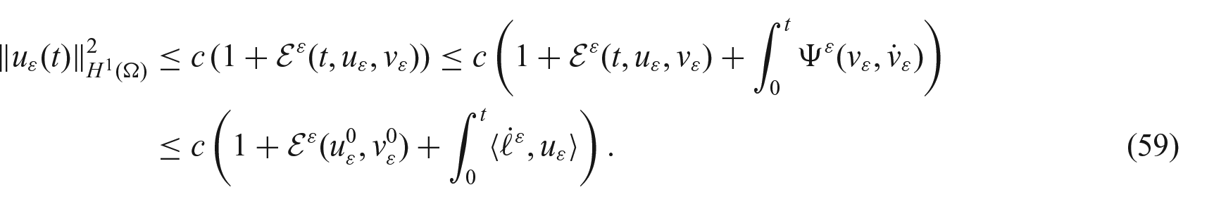
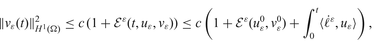
Thanks to Lemma 7.1 and the energy inequality (35), we have:

$$\begin{array}{c}\parallel u_{\epsilon }(t){\parallel }_{H^1(\mathrm{\Omega })}^2\le c(1+{\mathcal{E}}^{\epsilon }(t,u_{\epsilon },v_{\epsilon }))\le c(1+{\mathcal{E}}^{\epsilon }(t,u_{\epsilon },v_{\epsilon })+{\int }_0^t{\mathrm{\Psi }}^{\epsilon }(v_{\epsilon },{\stackrel{·}{v}}_{\epsilon }))\hfill \\ \le c(1+{\mathcal{E}}^{\epsilon }(u_{\epsilon }^0,v_{\epsilon }^0)+{\int }_0^t〈{\stackrel{·}{\ell }}^{\epsilon },u_{\epsilon }〉).\hfill \end{array}$$

(59)

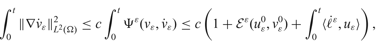
By the Gronwall Lemma [3, Lemma C.2.1, p. 534], this implies that $\parallel u_{\epsilon }(t){\parallel }_{H^1(\mathrm{\Omega })}\le c$ for every $t\in [0,T]$ .

Concerning $v_{\epsilon }$ , we similarly deduce from Lemma 7.1 that:

$$\parallel v_{\epsilon }(t){\parallel }_{H^1(\mathrm{\Omega })}^2\le c(1+{\mathcal{E}}^{\epsilon }(t,u_{\epsilon },v_{\epsilon }))\le c(1+{\mathcal{E}}^{\epsilon }(u_{\epsilon }^0,v_{\epsilon }^0)+{\int }_0^t〈{\stackrel{·}{\ell }}^{\epsilon },u_{\epsilon }〉),$$

so that $\parallel v_{\epsilon }(t){\parallel }_{H^1(\mathrm{\Omega })}\le c$ for every $t\in [0,T]$ , as well.

Again, by Lemma 7.1, we have $\parallel \nabla {\stackrel{·}{v}}_{\epsilon }(t){\parallel }_{L^2(\mathrm{\Omega })}^2\le c{\mathrm{\Psi }}^{\epsilon }(v_{\epsilon }(t),{\stackrel{·}{v}}_{\epsilon }(t))$ for every $t\in [0,T]$ . This yields:

$${\int }_0^t\parallel \nabla {\stackrel{·}{v}}_{\epsilon }{\parallel }_{L^2(\mathrm{\Omega })}^2\le c{\int }_0^t{\mathrm{\Psi }}^{\epsilon }(v_{\epsilon },{\stackrel{·}{v}}_{\epsilon })\le c(1+{\mathcal{E}}^{\epsilon }(u_{\epsilon }^0,v_{\epsilon }^0)+{\int }_0^t〈{\stackrel{·}{\ell }}^{\epsilon },u_{\epsilon }〉),$$

hence, $\parallel \nabla {\stackrel{·}{v}}_{\epsilon }{\parallel }_{L^2(0,T;L^2(\mathrm{\Omega }))}\le c$ . Therefore, up to a nonrelabeled subsequence, we find:

$$v_{\epsilon }(t)\rightharpoonup v(t)\mathrm{in}{H}^1(\mathrm{\Omega };{\mathbb{R}}^d),\nabla {\stackrel{·}{v}}_{\epsilon }(t)\rightharpoonup \nabla \stackrel{·}{v}(t)\mathrm{in}{L}^2(\mathrm{\Omega };{\mathbb{R}}^{d\times d}),$$

for almost every $t\in [0,T]$ . Notice that, since ${\mathcal{E}}^{\epsilon }(t,u_{\epsilon }(t),v_{\epsilon }(t))<\infty$ for every $t\in [0,T]$ , from assumption (L4) it follows $I+\epsilon \nabla v_{\epsilon }\in K$ for almost every $x\in \mathrm{\Omega }$ and for every $t\in [0,T]$ . In particular, $\epsilon \nabla v_{\epsilon }$ are uniformly bounded. Since $v_{\epsilon }\in {\mathcal{A}}_{\epsilon }$ by developing the determinant as a third-order polynomial, we get:

$$1=det(I+\epsilon \nabla v_{\epsilon })=1+\epsilon \mathrm{tr}\nabla v_{\epsilon }+{\epsilon }^2\mathrm{tr}(\mathrm{cof}\nabla v_{\epsilon })+{\epsilon }^{3}det\nabla v_{\epsilon }+\mathrm{o}({\epsilon }^4).$$

Using $\parallel \nabla v_{\epsilon }(t){\parallel }_{L^2(\mathrm{\Omega })}\le c$ and $\epsilon \parallel \nabla v_{\epsilon }(t){\parallel }_{L^{\infty }(\mathrm{\Omega })}\le c$ for a.e. $t\in (0,T)$ , we hence conclude that:

$$\parallel \mathrm{tr}\nabla v_{\epsilon }(t){\parallel }_{L^1(\mathrm{\Omega })}\le \epsilon \parallel \mathrm{tr}(\mathrm{cof}\nabla v_{\epsilon }(t)){\parallel }_{L^1(\mathrm{\Omega })}+{\epsilon }^2\parallel det\nabla v_{\epsilon }(t){\parallel }_{L^1(\mathrm{\Omega })}\le c\epsilon ,$$

for a.e. $t\in (0,T)$ . By passing to the limit as $\epsilon \to 0$ , this ensures that $\mathrm{tr}\nabla v=0$ a.e.

Fix now $t\in [0,T]$ . By equation (59), we have:

$$u_{\epsilon }(t)\rightharpoonup u(t)\mathrm{in}{H}^1(\mathrm{\Omega };{\mathbb{R}}^d),$$

(60)

where, at this point, the subsequence above may in general depend on $t$ . However, we will see that this is not the case by uniqueness of the limit (see the end of Section 7.3).

The linearized energy inequality (37) follows immediately from the energy inequality (35) at level $\epsilon$ , thanks to the $\lim \inf$ -inequalities in Lemma 7.3 and to the continuity of $\stackrel{·}{\ell }$ .

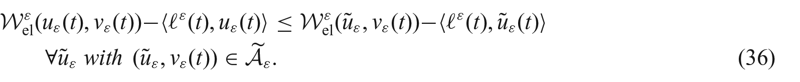
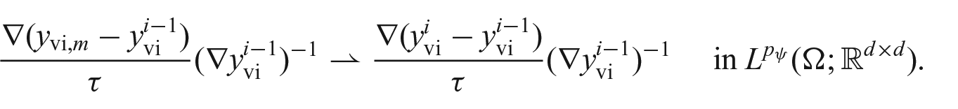
The linearized semistability condition (38), on the contrary, is more delicate, since it requires passing to the $\lim \sup$ on the right-hand side of the semistability condition (36) by choosing a suitable recovery sequence ${\tilde{u}}_{\epsilon }$ . In the following, we will drop the indication of the time dependence (note that time is fixed in this statement) and simply denote $u_{\epsilon }(t)=u_{\epsilon },v_{\epsilon }(t)=v_{\epsilon },u(t)=u$ , and $v(t)=v$ , to simplify notation.

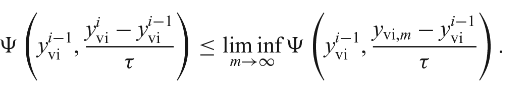
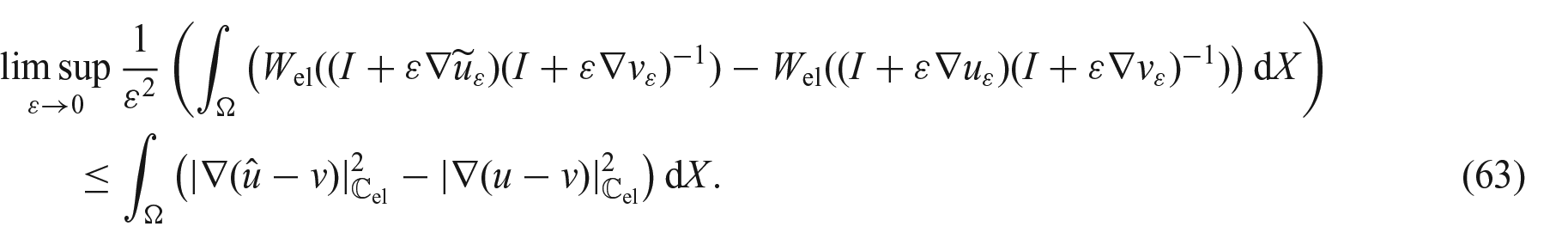
We start by showing that, for all fixed $\hat{u}\in H_{{\mathrm{\Gamma }}_D}^1(\mathrm{\Omega };{\mathbb{R}}^d)$ , one can choose a recovery sequence $({\tilde{u}}_{\epsilon }{)}_{\epsilon }$ such that:

$$0\stackrel{(36)}{\le }\underset{\epsilon \to 0}{\lim \sup }({\mathcal{W}}_{\mathrm{el}}^{\epsilon }({\tilde{u}}_{\epsilon },v_{\epsilon })-{\mathcal{W}}_{\mathrm{el}}^{\epsilon }(u_{\epsilon },v_{\epsilon }))\le {\mathcal{W}}_{\mathrm{el}}^0(\hat{u},v)-{\mathcal{W}}_{\mathrm{el}}^0(u,v).$$

(61)

With no loss of generality, we can assume by density that $\hat{u}$ has the form:

$$\hat{u}:=u+\tilde{u}\mathrm{where}\tilde{u}\in C_c^{\infty }(\mathrm{\Omega };{\mathbb{R}}^d).$$

As inequality (36) holds for every ${\tilde{u}}_{\epsilon }$ such that $({\tilde{u}}_{\epsilon },v_{\epsilon })\in {\tilde{A}}_{\epsilon }$ , i.e., ${\tilde{u}}_{\epsilon }\in H_{{\mathrm{\Gamma }}_D}^1(\mathrm{\Omega };{\mathbb{R}}^d)$ , we can choose:

$${\tilde{u}}_{\epsilon }:=\hat{u}+u_{\epsilon }-u=\tilde{u}+u_{\epsilon }.$$

Notice that we have:

$${\tilde{u}}_{\epsilon }-u_{\epsilon }=\tilde{u}\mathrm{and}{\tilde{u}}_{\epsilon }+u_{\epsilon }=\tilde{u}+2u_{\epsilon }\rightharpoonup \tilde{u}+2u\mathrm{in}{H}^1(\mathrm{\Omega };{\mathbb{R}}^d).$$

(62)

To check inequality (61), we need to show that:

$$\begin{array}{c}\underset{\epsilon \to 0}{\lim \sup }\frac{1}{{\epsilon }^2}\left({\int }_{\mathrm{\Omega }}(W_{\mathrm{el}}((I+\epsilon \nabla {\tilde{u}}_{\epsilon })(I+\epsilon \nabla v_{\epsilon }{)}^{-1})-W_{\mathrm{el}}((I+\epsilon \nabla u_{\epsilon })(I+\epsilon \nabla v_{\epsilon }{)}^{-1}))\mathrm{d}X\right)\hfill \\ \le {\int }_{\mathrm{\Omega }}(|\nabla (\hat{u}-v){|}_{{\mathbb{C}}_{\mathrm{el}}}^2-|\nabla (u-v){|}_{{\mathbb{C}}_{\mathrm{el}}}^2)\mathrm{d}X.\hfill \end{array}$$

(63)

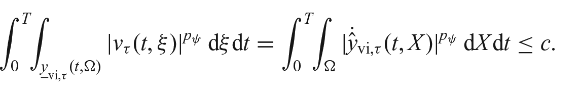
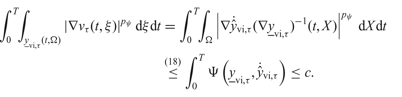
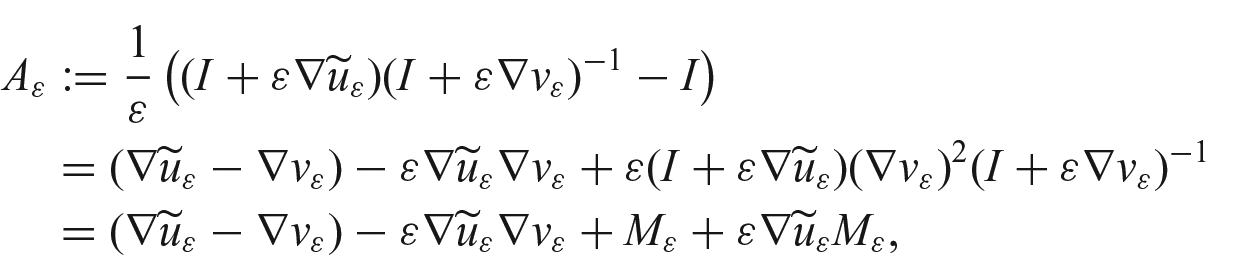
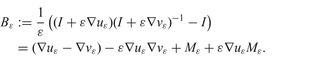
Let us first study the limiting behavior of the arguments of these energy densities. We define $(I+\epsilon \nabla {\tilde{u}}_{\epsilon })(I+\epsilon \nabla v_{\epsilon }{)}^{-1}=I+\epsilon A_{\epsilon }$ , namely,

$$\begin{array}{c}{A}_{\epsilon }:=\frac{1}{\epsilon }((I+\epsilon \nabla {\tilde{u}}_{\epsilon })(I+\epsilon \nabla v_{\epsilon }{)}^{-1}-I)\hfill \\ \multicolumn{1}{c}{=(\nabla {\tilde{u}}_{\epsilon }-\nabla v_{\epsilon })-\epsilon \nabla {\tilde{u}}_{\epsilon }\nabla v_{\epsilon }+\epsilon (I+\epsilon \nabla {\tilde{u}}_{\epsilon })(\nabla v_{\epsilon }{)}^2{(I+\epsilon \nabla v_{\epsilon })}^{-1}}\\ \multicolumn{1}{c}{=(\nabla {\tilde{u}}_{\epsilon }-\nabla v_{\epsilon })-\epsilon \nabla {\tilde{u}}_{\epsilon }\nabla v_{\epsilon }+M_{\epsilon }+\epsilon \nabla {\tilde{u}}_{\epsilon }{M}_{\epsilon },}\end{array}$$

where we have set $M_{\epsilon }:=\epsilon (\nabla v_{\epsilon }{)}^2(I+\epsilon \nabla v_{\epsilon }{)}^{-1}$ . Similarly, we can write $(I+\epsilon \nabla u_{\epsilon })(I+\epsilon \nabla v_{\epsilon }{)}^{-1}=I+\epsilon B_{\epsilon }$ by letting:

$$\begin{array}{c}{B}_{\epsilon }:=\frac{1}{\epsilon }((I+\epsilon \nabla u_{\epsilon })(I+\epsilon \nabla v_{\epsilon }{)}^{-1}-I)\hfill \\ \multicolumn{1}{c}{=(\nabla u_{\epsilon }-\nabla v_{\epsilon })-\epsilon \nabla u_{\epsilon }\nabla v_{\epsilon }+M_{\epsilon }+\epsilon \nabla u_{\epsilon }{M}_{\epsilon }.}\end{array}$$

Notice that by definition of $M_{\epsilon }$ and the fact that $I+\epsilon \nabla v_{\epsilon }\in K$ , we have:

$$\parallel \epsilon M_{\epsilon }{\parallel }_{L^{\infty }(\mathrm{\Omega })}\le c,\parallel M_{\epsilon }{\parallel }_{L^1(\mathrm{\Omega })}\le c\epsilon \parallel (\nabla v_{\epsilon }){\parallel }_{L^2(\mathrm{\Omega })}\le c\epsilon .$$

This implies by interpolation that $M_{\epsilon }$ is also bounded in $L^2(\mathrm{\Omega };{\mathbb{R}}^{d\times d})$ , hence $M_{\epsilon }\rightharpoonup 0$ weakly in $L^2(\mathrm{\Omega };{\mathbb{R}}^{d\times d})$ . Then, we have:

$$A_{\epsilon }-B_{\epsilon }=(\nabla {\tilde{u}}_{\epsilon }-u_{\epsilon })(I-\epsilon \nabla v_{\epsilon }+\epsilon M_{\epsilon })\stackrel{(62)}{=}\nabla \tilde{u}+\nabla \tilde{u}(-\epsilon \nabla v_{\epsilon }+\epsilon M_{\epsilon })\to \nabla \tilde{u}\mathrm{strongly}\mathrm{in}{L}^2(\mathrm{\Omega };{\mathbb{R}}^{d\times d}),$$

since $\nabla \tilde{u}\in C_c^{\infty }(\mathrm{\Omega };{\mathbb{R}}^{d\times d})$ is bounded in $L^{\infty }(\mathrm{\Omega };{\mathbb{R}}^{d\times d})$ and $(-\epsilon \nabla v_{\epsilon }+\epsilon M_{\epsilon })\to 0$ strongly in $L^2(\mathrm{\Omega };{\mathbb{R}}^{d\times d})$ . Moreover, by recalling equation (62), we have that:

$$A_{\epsilon }+B_{\epsilon }=(\nabla {\tilde{u}}_{\epsilon }+u_{\epsilon })(I-\epsilon \nabla v_{\epsilon }+\epsilon M_{\epsilon })-2(\nabla v_{\epsilon }-M_{\epsilon })\rightharpoonup \nabla \tilde{u}+2\nabla u-2\nabla v\mathrm{weakly}\mathrm{in}{L}^2(\mathrm{\Omega };{\mathbb{R}}^{d\times d}).$$

Fix now $\delta >0$ and let $c_{\mathrm{el}}(\delta )$ be as in assumption (28). Let us define the set:

$${\mathrm{\Omega }}_{\epsilon }^{\delta }:=\{x\in \mathrm{\Omega }|\epsilon |A_{\epsilon }|+\epsilon |B_{\epsilon }|\le c_{\mathrm{el}}(\delta )\},$$

containing all points where $\epsilon |A_{\epsilon }|$ and $\epsilon |B_{\epsilon }|$ are small. Notice that:

$$|\mathrm{\Omega }\backslash {\mathrm{\Omega }}_{\epsilon }^{\delta }|={\int }_{\mathrm{\Omega }\backslash {\mathrm{\Omega }}_{\epsilon }^{\delta }}1\mathrm{d}X\le \frac{{\epsilon }^2}{c_{\mathrm{el}}^2(\delta )}{\int }_{\mathrm{\Omega }}{(|A_{\epsilon }|+|B_{\epsilon }|)}^2\mathrm{d}X\le c\frac{{\epsilon }^2}{c_{\mathrm{el}}^2(\delta )}\to 0\mathrm{as}\epsilon \to 0,$$

(64)

since $A_{\epsilon }$ and $B_{\epsilon }$ are bounded in $L^2(\mathrm{\Omega };{\mathbb{R}}^{d\times d})$ . We split the integrals in the left-hand side of equation (63) in the sum of the integrals on the sets ${\mathrm{\Omega }}_{\epsilon }^{\delta }$ and on the complementary sets $\mathrm{\Omega }\backslash {\mathrm{\Omega }}_{\epsilon }^{\delta }$ . Using assumption (28) on the sets ${\mathrm{\Omega }}_{\epsilon }^{\delta }$ , we have:

$$\begin{array}{c}\frac{1}{{\epsilon }^2}{\int }_{{\mathrm{\Omega }}_{\epsilon }^{\delta }}(W_{\mathrm{el}}(I+\epsilon A_{\epsilon })-W_{\mathrm{el}}(I+\epsilon B_{\epsilon }))\mathrm{d}X\hfill \\ \le {\int }_{\mathrm{\Omega }}(|A_{\epsilon }{|}_{{\mathbb{C}}_{\mathrm{el}}}^2-|B_{\epsilon }{|}_{{\mathbb{C}}_{\mathrm{el}}}^2+\delta (|A_{\epsilon }{|}_{{\mathbb{C}}_{\mathrm{el}}}^2+|B_{\epsilon }{|}_{{\mathbb{C}}_{\mathrm{el}}}^2))\mathrm{d}X.\hfill \end{array}$$

(65)

The first term in the right-hand side above can be treated as follows:

$$\begin{array}{c}{\int }_{\mathrm{\Omega }}(|A_{\epsilon }{|}_{{\mathbb{C}}_{\mathrm{el}}}^2-|B_{\epsilon }{|}_{{\mathbb{C}}_{\mathrm{el}}}^2))\mathrm{dX}=\frac{1}{2}{\int }_{\mathrm{\Omega }}{\mathbb{C}}_{\mathrm{el}}(A_{\epsilon }+B_{\epsilon }):(A_{\epsilon }-B_{\epsilon }))\mathrm{d}X\hfill \\ \to \frac{1}{2}{\int }_{\mathrm{\Omega }}{\mathbb{C}}_{\mathrm{el}}((\nabla \hat{u}-\nabla v)+(\nabla u-\nabla v)):((\nabla \hat{u}-\nabla v)-(\nabla u-\nabla v))\mathrm{d}X\hfill \\ ={\int }_{\mathrm{\Omega }}(|\nabla (\hat{u}-v){|}_{{\mathbb{C}}_{\mathrm{el}}}^2-|\nabla (u-v){|}_{{\mathbb{C}}_{\mathrm{el}}}^2)\mathrm{d}X,\hfill \end{array}$$

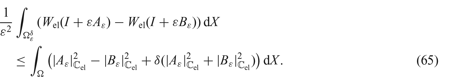
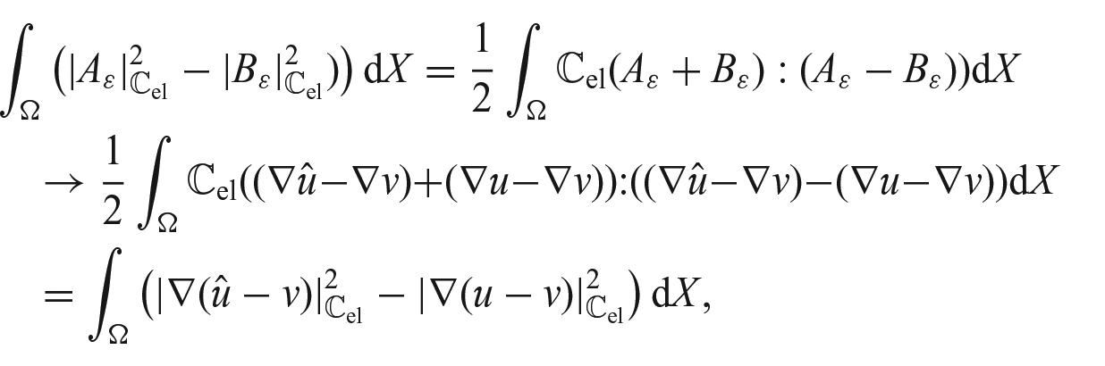
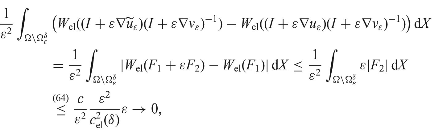
by means of the strong convergence of $A_{\epsilon }-B_{\epsilon }\to \nabla \tilde{u}$ and the weak convergence of $A_{\epsilon }+B_{\epsilon }\rightharpoonup \nabla \tilde{u}+2\nabla u-2\nabla v$ in $L^2(\mathrm{\Omega };{\mathbb{R}}^{d\times d})$ . On the contrary, the second term in the right-hand side of equation (65) satisfies:

$${\int }_{\mathrm{\Omega }}\delta (|A_{\epsilon }{|}_{{\mathbb{C}}_{\mathrm{el}}}^2+|B_{\epsilon }{|}_{{\mathbb{C}}_{\mathrm{el}}}^2)\mathrm{dX}\le \delta c,$$

since $A_{\epsilon }$ and $B_{\epsilon }$ are bounded in $L^2(\mathrm{\Omega };{\mathbb{R}}^{d\times d})$ .

Hence, it remains to show that the integrals in equation (63) on the complements $\mathrm{\Omega }\backslash {\mathrm{\Omega }}_{\epsilon }^{\delta }$ converge to $0$ as $\epsilon \to 0$ . In order to do so, let us define:

$$F_1:=(I+\epsilon \nabla u_{\epsilon })(I+\epsilon \nabla v_{\epsilon }{)}^{-1}{F}_2:=\nabla \tilde{u}(I+\epsilon \nabla v_{\epsilon }{)}^{-1}.$$

Since by definition $\nabla {\tilde{u}}_{\epsilon }=\nabla \tilde{u}+\nabla u_{\epsilon }$ and $W$ is locally Lipschitz, we can write:

$$\begin{array}{c}\frac{1}{{\epsilon }^2}{\int }_{\mathrm{\Omega }\backslash {\mathrm{\Omega }}_{\epsilon }^{\delta }}(W_{\mathrm{el}}((I+\epsilon \nabla {\tilde{u}}_{\epsilon })(I+\epsilon \nabla v_{\epsilon }{)}^{-1})-W_{\mathrm{el}}((I+\epsilon \nabla u_{\epsilon })(I+\epsilon \nabla v_{\epsilon }{)}^{-1}))\mathrm{d}X\hfill \\ \multicolumn{1}{c}{=\frac{1}{{\epsilon }^2}{\int }_{\mathrm{\Omega }\backslash {\mathrm{\Omega }}_{\epsilon }^{\delta }}|W_{\mathrm{el}}(F_1+\epsilon F_2)-W_{\mathrm{el}}(F_1)|\mathrm{d}X\le \frac{1}{{\epsilon }^2}{\int }_{\mathrm{\Omega }\backslash {\mathrm{\Omega }}_{\epsilon }^{\delta }}\epsilon |F_2|\mathrm{d}X}\\ \multicolumn{1}{c}{\stackrel{(64)}{\le }\frac{c}{{\epsilon }^2}\frac{{\epsilon }^2}{c_{\mathrm{el}}^2(\delta )}\epsilon \to 0,}\end{array}$$

where we used that $F_2$ is uniformly bounded in $L^{\infty }(\mathrm{\Omega };{\mathbb{R}}^{d\times d})$ . This concludes the proof of inequality (63). The check of linearized semistability (38) then follows as soon as one passes to the limit in the loading terms, which is straightforward.

In particular, we have proved that $u$ solves the linear minimization problem:

$${\mathcal{W}}_{\mathrm{el}}^0(u(t),v(t))-〈{\ell }^0(t),u(t)〉=\underset{\hat{u}\in H_{{\mathrm{\Gamma }}_D}^1(\mathrm{\Omega };{\mathbb{R}}^d)}{\arg \min }{\mathcal{W}}_{\mathrm{el}}^0(\hat{u},v(t))-〈{\ell }^0(t),\hat{u}〉,$$

for given $v$ , thanks to equation (38). Hence, the limit $u$ is unique and measurable in time, since it is the image of $v$ through a linear operator. We also remark that this implies that subsequences in equation (60) can be chosen independently of $t$ .