An internal variable model of macroscopic twin boundary dynamics

Abstract

Depending on whether the experiments are quasi-static or fast dynamics, the measured twin boundary velocity values range from zero to the material’s sound speed. The twin boundary velocity is not yet predicted theoretically in the continuum mechanics framework. The extension of continual description is provided in the paper by means of internal variables. It is shown that a diffusional slow motion of twin boundaries can be represented using a single internal variable. The dual internal variable technique is employed for the description of the fast dynamics of twin boundaries.

1. Introduction

Twins are planar defects of the crystal lattice that can be represented as coherent interfaces between identical but differently oriented lattices. One of the most essential features of twins is their ability to move in response to external forces, which results in growth of one of the differently oriented lattices and carries a macroscopic deformation of the material. Twin boundary motion is especially essential in shape memory alloys [1,2], where the twins appear between different variants of martensite. The reversible reorientation of martensite via twins motion is the key mechanism of pseudoplastic straining of shape memory alloys, and the speed of this process can be decisive for the overall mechanical performance of the alloy.

The study of mechanical twins has a long history [3]. For a long time, it was considered that twins grew at exceptionally rapid rates due to audible sounds detected during the twinning process [4,5]. The rapid growth of twins has been confirmed by experiments by Takeuchi [6] who reported the value 2570 m/s for twin head velocity in iron single crystals, by Williams and Reid [7] with 2250 m/s for the velocity of twin tip in silicon–iron alloy, and by recent in situ high-speed optical imaging of twin tip propagation in single crystal magnesium reaching 2000 m/s [8].

Furthermore, the theoretical prediction by Rosakis and Tsai [9] of possibly intersonic twin development was confirmed experimentally for ferroelectric crystals [10] and for single-crystal aluminum [11]. Bowden and Cooper [12], on the contrary, reported that the observed velocity of twin propagation in zinc crystals under explosive loading ranged from 30 to 300 m/s. In situ measurements of twin boundary motion by Smith et al. [13] in the magnetic shape memory alloy Ni–Mn–Ga gave a value of 82.5 m/s for the twin boundary velocity. The twin boundary velocity in Ni–Mn–Ga 5M martensite recorded with a high-speed camera was determined to be 39 m/s [14].

However, this is not the smallest experimentally recorded value for the velocity of the twin boundary. According to Mizrahi et al. [15], dynamic force pulse tests on a 10M Ni–Mn–Ga single crystal produced twin boundary velocity values ranging from 0 to 14 m/s. Furthermore, the twin boundary velocity in a slow-rate experiment is typically ${10}^{-5}\mathrm{m}/\mathrm{s}$ , as mentioned in [16].

The significant scatter in the experimental data requires a better understanding of the dynamics of twin boundaries. Various aspects of twin boundary motion have been studied theoretically and computationally. Phase-field models (c.f. [17–20]), crystal plasticity model (e.g., [21]), and their combinations [22, 23] do not consider individual twin boundaries. Quasi-static micromechanics-based models [16, 24–26] are concentrated on their own experimental data. Fast moving twin boundaries (e.g., [27, 28]) are beyond the scope of models by Faran and Shilo.

The common approach to the continuum description of twin boundaries, and phase fronts in diffusionless phase transitions in general, is to assume a multiwell energy landscape $W(u_x)$ , where individual minima on the strain energy density represent the individual equilibrium states or variants. This approach, however, requires either dealing with higher-order polynomials for the elastic energy (the Landau-energy landscape framework, c.f., [29–32]) or assuming the energy landscape as piecewise quadratic with discontinuity in second derivatives [33]. In both cases, issues about the nature and height of the barrier between the energy wells arise, and the velocity of phase boundaries cannot be predicted uniquely. As a result, the continuum description of twin boundary propagation is incomplete. The incompleteness is resolved using a special Landau functional structure [34] or a kinetic relation [33]. In both cases, additional constitutive assumptions are introduced.

A new approach is provided by the dual internal variable theory [35–38]. This study reveals how to model both slow and fast twin boundary propagation in the continuum mechanics framework enhanced by dual internal variables. For simplicity, we focus on a uniaxial situation with a scalar transverse displacement field $u(x)$ , where two lattices distinguished by one-dimensional shear strains $u_x=\pm {\epsilon }^{\mathrm{tr}}/2$ . We will hereafter refer to these two lattices as to twins.

1.1. Uniaxial twin boundary motion

Uniaxial motion implies that all fields are dependent on a single coordinate and time. Longitudinal and transverse motions are uncoupled in the uniaxial setting. We disregard longitudinal motion by focusing on shear strains. Restricting by the transverse displacement $u$ :

$$u=u(x,t),$$

(1)

we apply the balance of linear momentum in the isothermal case (without body forces) as:

$$\rho v_t={\sigma }_x,$$

(2)

where $\sigma$ is the shear stress, $v=u_t$ is the transverse particle velocity, $\rho$ is the constant matter density, and subscripts denote the derivatives. The kinematic compatibility condition reads:

$${\epsilon }_t=v_x,$$

(3)

where $\epsilon =u_x$ is the shear strain.

1.2. Jump conditions

Let the possibly moving twin boundary $\mathcal{S}$ splitting the variants be located at a certain position $x_0$ . The following jump relation is satisfied at this boundary in the context of the continuum description (e.g., [33]):

$$V_N\left[\left[\rho v\right]\right]+\left[\left[\sigma \right]\right]=0,$$

(4)

where $V_N$ is the velocity of the moving twin boundary, and $\left[\left[B\right]\right]=B^{+}-B^{-},B^{\pm }$ are the uniform limits of a field $B$ in approaching the boundary from its positive and negative sides, respectively.

The driving force $f_{\mathcal{S}}$ acting on the boundary is determined by Abeyaratne and Knowles [33]:

$$f_{\mathcal{S}}=\left[\left[W\right]\right]-〈\sigma 〉\left[\left[\epsilon \right]\right],$$

(5)

where $W$ is the free energy per unit volume and 〈…〉 denotes the arithmetical mean.

1.3. Twin boundary velocity

The velocity of the twin boundary is determined by the relationship:

$$\rho V_N^2\left[\left[\epsilon \right]\right]=\left[\left[\sigma \right]\right],$$

(6)

which follows from jump relation (4) and that for the jump of the kinematic compatibility condition (3):

$$\left[\left[v\right]\right]=-\left[\left[\epsilon \right]\right]V_N.$$

(7)

The sign of the velocity of the twin boundary follows from the entropy inequality on the twin boundary [33]:

$$f_{\mathcal{S}}{V}_N\ge 0.$$

(8)

It should be noted that the lack of uniqueness exists for the relevant initial-boundary value problem [39] since the stress jump in equation (6) is not known in advance.

1.4. Isothermal twins equilibrium

We consider a material with two possible twin variants. We assume that the variants are energetically equivalent, which means that material points in both variants have the same energy value. It is also assumed that the elastic parameters for both variants are the same. In uniaxial setting, the elastic free energy per unit volume is the quadratic function of shear strain:

$$W=\frac{G}{2}{u}_x^2,$$

(9)

where $G$ is the shear modulus of the material, and subscript denotes the space derivative. It is obvious that the energy value is the same for $+u_x$ and $-u_x$ .

Assume the variants occupy adjacent parts of a body separated by a twin boundary. We will investigate the conditions for the coexistence of the variants in equilibrium state. Although the equilibrium state implies that there is no motion ( $u=0$ ), shear strains can have non-zero values in both variants. Positive strains are associated with variant 1 and negative strains with variant 2. It is well known that the strains in distinct twins differ from one another by the so-called transformation strain ${\epsilon }^{\mathrm{tr}}$ . Because of the symmetry, the shear strain values can be specified as follows:

$${\epsilon }_1=\frac{1}{2}{\epsilon }^{\mathrm{tr}},{\epsilon }_2=-\frac{1}{2}{\epsilon }^{\mathrm{tr}}.$$

(10)

This keeps the equality of the free energy in both variants. Here, lower indices indicate twin variants.

It is reasonable to assume that in equilibrium, the value of stress is equal to zero. However, the stress is linear in strain:

$$\sigma =\frac{\partial W}{\partial \epsilon }=G\epsilon ,$$

(11)

which leads to the following values of the stress in distinct variants:

$${\sigma }_1=G{\epsilon }_1=\frac{G}{2}{\epsilon }^{\mathrm{tr}},{\sigma }_2=G{\epsilon }_2=-\frac{G}{2}{\epsilon }^{\mathrm{tr}}.$$

(12)

It follows that the stress equality cannot be achieved in the macroscopic representation.

As a result, the macroscopic exposition encounters problems with both equilibria of twins and twin boundary motion. It is clear that the continuum description of twin boundary dynamics should be expanded. We will employ internal variables to increase the degree of freedom in the representation.

1.5. Internal variables

The idea of the use of internal variables is not new. It has been exploited intensively in the modeling of shape memory alloys [40–44]. As a rule, individual phase boundaries were not considered because the internal variable was the martensitic volume fraction with a prescribed transformation kinetics [45–47]. Variants of transformation kinetics have been reviewed in Paiva and Savi [48] and Khandelwal and Buravalla [49].

This paper employs another internal variable approach [36–38]. Here, internal variables characterize the difference between twins. This makes it possible to use them to identify twin boundaries. Basic notions of this internal variables method are presented in Appendix 1.

Internal variables allow us to avoid non-convexity and/or non-smoothness in the energy density function $W(u_x)$ by introducing extra degrees of freedom. We start with a single internal variable case. Here, we assume that the elastic response of each twin variant is governed by a quadratic energy well with a switching parameter that specifies in which variant the material is. This parameter is the gradient of the internal variable. The free energy per unit volume is then represented as:

$$W(u_x,{\phi }_x)=\frac{G}{2}{u}_x^2+\frac{1}{2}A{u}_x{\phi }_x+\frac{1}{2}C{\phi }_x^2,$$

(13)

where $A$ and $C$ are the constants, and $\phi$ is the internal variable. For setting $A=G{\epsilon }^{\mathrm{tr}}$ , the stress is determined in the form:

$$\sigma =\frac{\partial W}{\partial u_x}=G(u_x+\frac{1}{2}{\epsilon }^{\mathrm{tr}}{\phi }_x),$$

(14)

which enables switching between two stress-free states with $u_x={\epsilon }^{\mathrm{tr}}/2$ and $u_x=-{\epsilon }^{\mathrm{tr}}/2$ , respectively, by setting the parameter ${\phi }_x$ equal to $-1$ and 1. These two states represent the two energy minima associated with two twin variants. In section 3, we will demonstrate that this formalism can capture the slow dynamics response of the system to quasi-static loading.

For fast dynamics, where the inertia of the material is essential, we show that the propagation of a twin boundary can be described using a dual variable model (section 4), assuming the energy density function of form:

$$W(u_x,{\phi }_x,\psi )=\frac{G}{2}{u}_x^2+\frac{1}{2}A{u}_x{\phi }_x-\frac{1}{2}C{\phi }_x^2-\frac{1}{2}D{\psi }^2,$$

(15)

where the last term with the dual internal variable $\psi$ ensures that the evolution equations for the internal variables are in this case hyperbolic, as elaborated in detail in Appendix 1. As a result, wave-like propagating solutions for the switching parameter ${\phi }_x$ allow fast-moving, inertia-driven twin boundaries.

2. Single internal variable

In the single internal variable case, the free energy $W$ per unit volume is specified as a quadratic function of the shear strain, the internal variable, $\phi$ , and its space gradient ${\phi }_x$ (e.g., [50]):

$$W=\frac{G}{2}{u}_x^2+\frac{1}{2}A{u}_x{\phi }_x+\frac{1}{2}C{\phi }_x^2,$$

(16)

with material parameters $A=G{\epsilon }^{\mathrm{tr}}$ and $C$ . We consider here a reduced version of the free energy dependence because only the gradient of internal variable is included.

To distinguish twin variants, we suppose that internal variable gradients have alternating signs. If for the variant 1 we assume the negative sign of the gradient of internal variable, then for variant 2 it should be positive.

By definition, the shear stress is calculated as:

$$\sigma =\frac{\partial W}{\partial u_x}=G(u_x+\frac{1}{2}{\epsilon }^{\mathrm{tr}}{\phi }_x).$$

(17)

If ${\phi }_x=-1$ , then the value of the shear stress:

$${\sigma }_1=G({(u_x)}_1-\frac{1}{2}{\epsilon }^{\mathrm{tr}}),$$

(18)

corresponds to variant 1. For variant 2, we have, accordingly, ${\phi }_x=1$ and:

$${\sigma }_2=G({(u_x)}_2+\frac{1}{2}{\epsilon }^{\mathrm{tr}}).$$

(19)

2.1. Equilibrium conditions

To be more specific, let us consider the uniaxial state of a bar which may contain two kinds of twin variants. The bar occupies the region $0<x<L$ . Suppose that variant 1 occupies the part of the bar $0<x<l_1$ and variant 2 is in the rest of the bar. The state of each twin variant is determined by the values of shear strains ${\epsilon }_1$ and ${\epsilon }_2$ and gradients of internal variable $({\phi }_1{)}_x={\gamma }_1$ and $({\phi }_2{)}_x={\gamma }_2$ . It is reasonable to assume that both twins are stress-free in equilibrium. The following shear strain values relate to zero stress levels:

$${\epsilon }_1=\frac{1}{2}{\epsilon }^{\mathrm{tr}},{\epsilon }_2=-\frac{1}{2}{\epsilon }^{\mathrm{tr}}.$$

(20)

Accordingly, the driving force acting at the twin boundary reduces to the jump of the free energy in the stress-free equilibrium:

$$f_{\mathcal{S}}=\left[\left[W\right]\right]-〈\sigma 〉\left[\left[\epsilon \right]\right]=\left[\left[W\right]\right].$$

(21)

Calculating the free energy jump:

$$\begin{array}{c}(W_2-W_1)=(\frac{G}{2}{\epsilon }_2^2+\frac{1}{2}A{\epsilon }_2{\gamma }_2+\frac{1}{2}C{\gamma }_2^2)-\hfill \\ \multicolumn{1}{c}{-(\frac{G}{2}{\epsilon }_1^2+\frac{1}{2}A{\epsilon }_1{\gamma }_1+\frac{1}{2}C{\gamma }_1^2)=}\\ \multicolumn{1}{c}{=\frac{G}{2}({\epsilon }_2^2-{\epsilon }_1^2)+\frac{1}{2}G{\epsilon }^{\mathrm{tr}}({\epsilon }_2{\gamma }_2-{\epsilon }_1{\gamma }_1)+\frac{1}{2}C({\gamma }_2^2-{\gamma }_1^2)+{\sigma }_0{\epsilon }^{\mathrm{tr}}=}\\ \multicolumn{1}{c}{=\frac{G}{2}({\epsilon }_2-{\epsilon }_1)({\epsilon }_2+{\epsilon }_1)+\frac{1}{2}G{\epsilon }^{\mathrm{tr}}({\epsilon }_2{\gamma }_2-{\epsilon }_1{\gamma }_1)+}\\ \multicolumn{1}{c}{+\frac{C}{2}({\gamma }_2-{\gamma }_1)({\gamma }_2+{\gamma }_1)=0,}\end{array}$$

(22)

we obtain zero value because of conditions ${\epsilon }_1+{\epsilon }_2=0$ and ${\gamma }_2+{\gamma }_1=0$ . As a result, there is no driving force at the twin boundary in equilibrium, as expected. Thus, the introduction of the internal variable enables the twins to achieve a stress-free equilibrium. The obtained relationships serve as initial conditions for a possible motion of the twin boundary.

3. Slow motion

To determine a possible motion of the twin boundary, we need to calculate the value of the driving force in non-equilibrium:

$$\begin{array}{c}{f}_{\mathcal{S}}=\left[\left[W\right]\right]-〈\sigma 〉\left[\left[\epsilon \right]\right]=(\frac{G}{2}{\epsilon }_2^2+\frac{1}{2}A{\epsilon }_2{\gamma }_2+\frac{1}{2}C{\gamma }_2^2)-\hfill \\ \multicolumn{1}{c}{-(\frac{G}{2}{\epsilon }_1^2+\frac{1}{2}A{\epsilon }_1{\gamma }_1-\frac{1}{2}C{\gamma }_1^2)-\frac{1}{2}({\sigma }_2+{\sigma }_1)({\epsilon }_2-{\epsilon }_1)=}\\ \multicolumn{1}{c}{=\frac{G}{2}({\epsilon }_2^2-{\epsilon }_1^2)+\frac{1}{2}G{\epsilon }^{\mathrm{tr}}({\epsilon }_2{\gamma }_2-{\epsilon }_1{\gamma }_1)+\frac{1}{2}C({\gamma }_2^2-{\gamma }_1^2)+}\\ \multicolumn{1}{c}{+\frac{1}{2}(G({\epsilon }_2+\frac{1}{2}{\epsilon }^{\mathrm{tr}}{\gamma }_2)+G({\epsilon }_1+\frac{1}{2}{\epsilon }^{\mathrm{tr}}{\gamma }_1))({\epsilon }_2-{\epsilon }_1)=}\\ \multicolumn{1}{c}{=\frac{1}{2}G{\epsilon }^{\mathrm{tr}}({\epsilon }_2{\gamma }_2-{\epsilon }_1{\gamma }_1)+\frac{1}{2}C({\gamma }_2^2-{\gamma }_1^2)+\frac{1}{2}G{\epsilon }^{\mathrm{tr}}〈\gamma 〉({\epsilon }_2-{\epsilon }_1),}\end{array}$$

(23)

which is non-zero anymore. The twin boundary velocity is then determined as:

$$V_N^2=\frac{\left[\left[\sigma \right]\right]}{\rho \left[\left[\epsilon \right]\right]}=\frac{G({\epsilon }_2+\frac{1}{2}{\epsilon }^{\mathrm{tr}}{\gamma }_2)-G({\epsilon }_1+\frac{1}{2}{\epsilon }^{\mathrm{tr}}{\gamma }_1)}{\rho \left[\left[\epsilon \right]\right]}=\frac{G}{\rho }(1+\frac{{\epsilon }^{\mathrm{tr}}}{\left[\left[\epsilon \right]\right]}\frac{{\gamma }_2-{\gamma }_1}{2}).$$

(24)

If the value of the driving force exceeds a certain threshold, the boundary between the twins is expected to shift. The change of twin state is governed by the dimensionless balance of linear momentum:

$${\overline{v}}_t={\overline{\epsilon }}_x+\frac{A}{2G}{\overline{\gamma }}_x,$$

(25)

and the evolution equation for the internal variable:

$${\overline{\gamma }}_t=\frac{C}{A}{\overline{\gamma }}_{\mathrm{xx}}+\frac{1}{2}{\overline{\epsilon }}_{\mathrm{xx}}.$$

(26)

Details of the derivation of the evolution equation for the gradient of the internal variable are given in Appendix 1. The gradient of the internal variable can be interpreted as an order parameter because its evolution equation is of the Ginzburg–Landau type. It should be noted that equations (25) and (26) are coupled and non-reflecting boundary conditions are applied at ends of the bar.

3.1. Numerical example

For the numerical test, the length of the bar is divided by 1000 space steps. The boundary between twins is placed at the point corresponding to 400 space steps. The left part of the specimen is occupied by the variant 1 (marked by yellow color in Figure 1).

Figure 1.

Sketch of initial twins position.

The values of shear strains in twins are chosen as follows:

$${\epsilon }_1=0.02,{\epsilon }_2=-0.02,{\epsilon }^{\mathrm{tr}}=0.04.$$

(27)

Gradients of the internal variable follow conditions:

$${\gamma }_1=-1,{\gamma }_2=1.$$

(28)

The choice of the parameters corresponds to an equilibrium state with zero shear stress value. Initial distributions of shear strains and gradients of the internal variable are illustrated in Figures 2 and 3.

Figure 2.

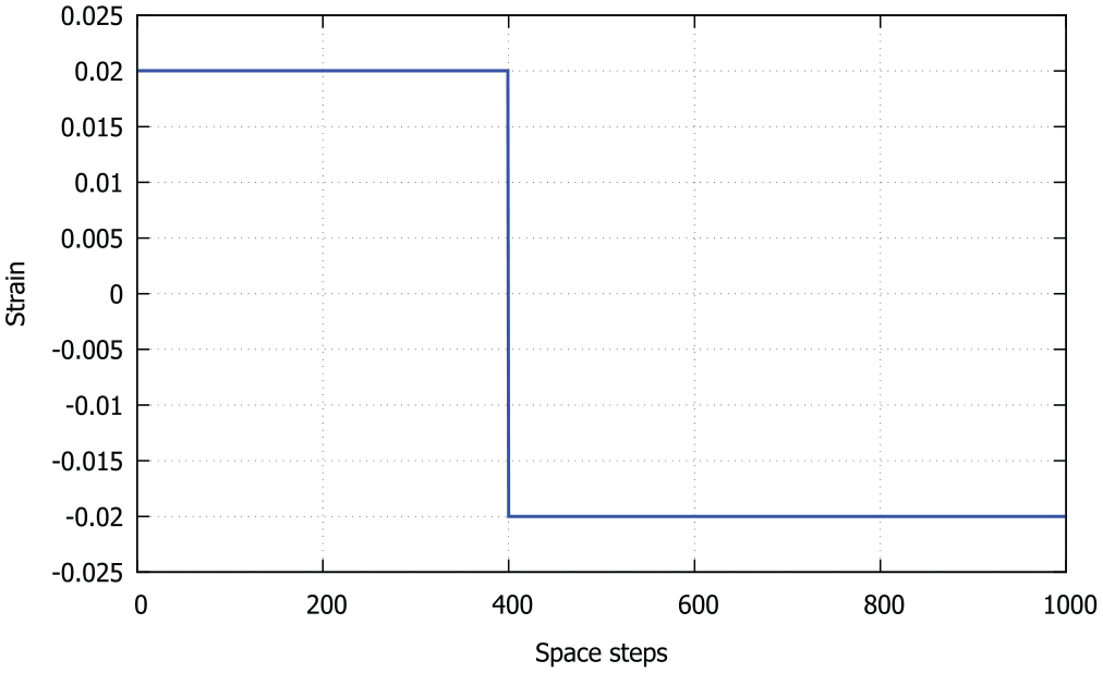
Equilibrium shear strain distribution.

Figure 3.

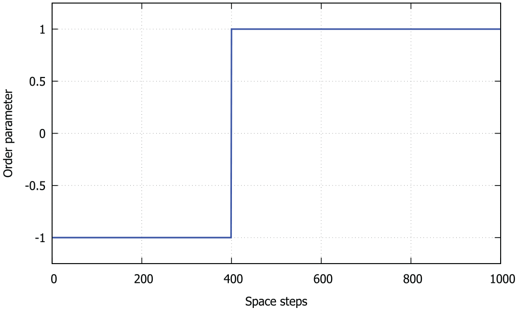
Equilibrium distribution of the gradient of the internal variable $\gamma$ .

It is clear that the equilibrium state will not change in the absence of external influence. Consider now the situation where the variant 1 (as a whole) receives an additional amount of energy from external sources. The time history of the loading is shown in Figure 4. Suppose that this additional energy leads to the value of the driving force above the critical value. The placement of the boundary between variants will change accordingly.

Figure 4.

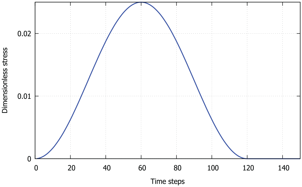
Shear stress variation in time in the variant 1.

The twin boundary motion is simulated numerically. Starting with the initial equilibrium state shown in Figures 2 and 3, new shear strains and gradients of the internal variable are computed in each time step solving equations (25) and (26). Computations are performed by the thermodynamically consistent finite volume numerical scheme [51]. The main feature of the used scheme is the ability to determine the value of the stress jump at the moving boundary algorithmically [51]. This eliminates the non-uniqueness in the solution. The corresponding driving force and a possible velocity of the twin boundary are calculated following equations (23) and (24). The motion of the twin boundary is allowed only if the value of the driving force overcomes a critical value.

The twin boundary motion is manifested by the change in the distributions of shear strain and gradient of the internal variable at different time instants as shown in Figures 5 and 6. The distribution of the shear strain is plotted sequentially for every 50 time steps in Figure 5, beginning with that for 50 time steps. The shifted shape of the shear strain distribution is clearly visible. The upper line represents the new equilibrium state.

Figure 5.

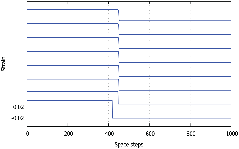
Shift of the shear strain distribution over time.

Figure 6.

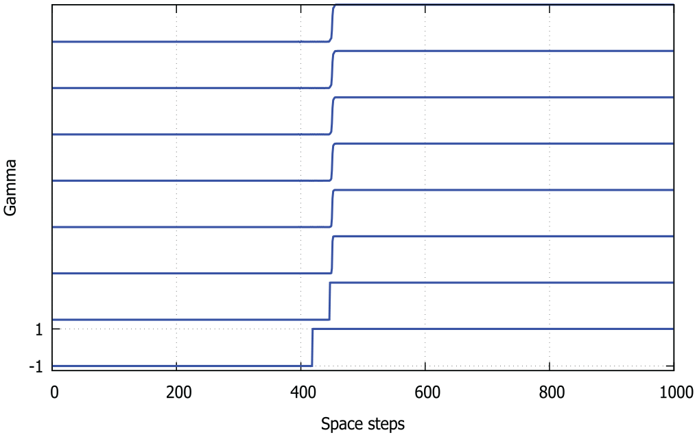
Change in the distribution of the gradient of the internal variable over time.

A similar plot for the distribution of the gradient of the internal variable is displayed in Figure 6. It is noteworthy that the gradient of the internal variable exhibits typical order parameter behavior.

The results of the calculation of the variation of the position of the twin boundary over time are shown in Figure 7. The position of the twin boundary changes nonlinearly in response to the external load from its initial value (400 space steps) to a final one. It corresponds to the shift in shear strain and gradient of internal variable presented in Figures 5 and 6. After the external loading is reduced, the twin boundary stops moving.

Figure 7.

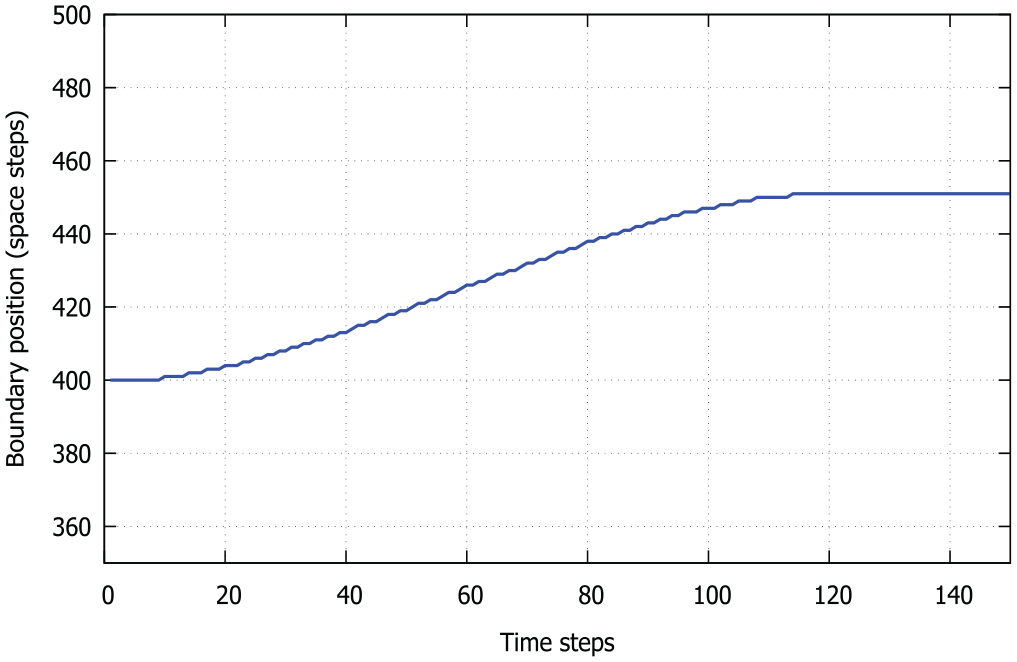
Variation of the position of the twin boundary in time.

The dependence of the velocity of the twin boundary on the driving force is presented in Figure 8. It represents a typical kinetic relation curve.

Figure 8.

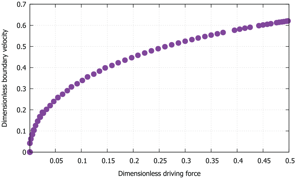
Boundary velocity versus driving force.

3.2. Asymptotics of the strain jump

For a small deviation of the actual shear strain jump from the value of the transformation strain, we can represent the shear strain jump as an asymptotic expansion:

$$\left[\left[\epsilon \right]\right]={\epsilon }^{\mathrm{tr}}(1+\delta {ϵ}^1+\dots ),$$

(29)

with a small parameter $\delta$ .

In such a case, the velocity of the twin boundary is, in the first approximation:

$$V_N^2=\frac{G}{\rho }(1+\frac{{\epsilon }^{\mathrm{tr}}}{\left[\left[\epsilon \right]\right]}\frac{{\gamma }_2-{\gamma }_1}{2})\approx \frac{G}{\rho }\delta {ϵ}^1,$$

(30)

because the value of ${\gamma }_2-{\gamma }_1$ is close to 2 in the vicinity of twin boundary. It is clear that the value of the twin boundary velocity can be as small as that dictated by the value of $\delta$ in a particular situation. The slow motion of the twin boundary corresponding to the single internal variable model correlates to results of quasi-static experiments [15, 16, 24, 52]. However, the single internal variable model is insufficient for fast dynamics of twin boundaries because it exploits a parabolic evolution equation for the internal variable.

4. Fast dynamics

4.1. Dual internal variables

We apply the dual internal variable approach [36, 37] to go beyond the diffusional description. The complete theory of dual internal variables is presented in Berezovski and Ván [36]. Here, we use a reduced version of the theory assuming that the free energy density depends on internal variables $\phi$ and $\psi$ by virtue of a quadratic function:

$$W=\frac{G}{2}{u}_x^2+\frac{1}{2}A{\phi }_x{u}_x-\frac{1}{2}C{\phi }_x^2-\frac{1}{2}D{\psi }^2,$$

(31)

where material parameters $A=G{\epsilon }^{\mathrm{tr}}$ , $C$ , and $D$ are constant. In this version, the free energy does not depend on the internal variable $\phi$ explicitly and on the gradient of the internal variable $\psi$ . Negative signs for coefficients $C$ and $D$ are applied in the correspondence to Berezovski [53].

Shear stress values are calculated as previously:

$$\sigma =\frac{\partial W}{\partial u_x}=G(u_x+\frac{1}{2}{\epsilon }^{\mathrm{tr}}{\phi }_x).$$

(32)

4.2. Driving force and twin boundary velocity

In the case of dual internal variables, the expression for the driving force takes the form:

$$\begin{array}{c}{f}_{\mathcal{S}}=\left[\left[W\right]\right]-〈\sigma 〉\left[\left[\epsilon \right]\right]=(\frac{G}{2}{\epsilon }_2^2+\frac{1}{2}A{\epsilon }_2{\gamma }_2-\frac{1}{2}C{\gamma }_2^2-\frac{1}{2}D{\psi }_2^2)-\hfill \\ \multicolumn{1}{c}{-(\frac{G}{2}{\epsilon }_1^2+\frac{1}{2}A{\epsilon }_1{\gamma }_1-\frac{1}{2}C{\gamma }_1^2-\frac{1}{2}D{\psi }_1^2)-\frac{1}{2}({\sigma }_2+{\sigma }_1)({\epsilon }_2-{\epsilon }_1)=}\\ \multicolumn{1}{c}{=\frac{G}{2}({\epsilon }_2^2-{\epsilon }_1^2)+\frac{1}{2}G{\epsilon }^{\mathrm{tr}}({\epsilon }_2{\gamma }_2-{\epsilon }_1{\gamma }_1)-\frac{1}{2}C({\gamma }_2^2-{\gamma }_1^2)-}\\ \multicolumn{1}{c}{-\frac{1}{2}D({\psi }_2^2-{\psi }_1^2)-\frac{1}{2}(G({\epsilon }_2+\frac{1}{2}{\epsilon }^{\mathrm{tr}}{\gamma }_2)+G({\epsilon }_1+\frac{1}{2}{\epsilon }^{\mathrm{tr}}{\gamma }_1))({\epsilon }_2-{\epsilon }_1)=}\\ \multicolumn{1}{c}{=\frac{1}{2}G{\epsilon }^{\mathrm{tr}}({\epsilon }_2{\gamma }_2-{\epsilon }_1{\gamma }_1)-C\left[\left[\gamma \right]\right]〈\gamma 〉-D\left[\left[\psi \right]\right]〈\psi 〉-\frac{1}{2}G{\epsilon }^{\mathrm{tr}}〈\gamma 〉\left[\left[\epsilon \right]\right].}\end{array}$$

(33)

The value of the twin boundary velocity is calculated accordingly:

$$V_N^2=\frac{\left[\left[\sigma \right]\right]}{\rho \left[\left[\epsilon \right]\right]}=\frac{G({\epsilon }_2+\frac{1}{2}{\epsilon }^{\mathrm{tr}}{\gamma }_2)-G({\epsilon }_1+\frac{1}{2}{\epsilon }^{\mathrm{tr}}{\gamma }_1)}{\rho \left[\left[\epsilon \right]\right]}=\frac{G}{\rho }(1+\frac{{\epsilon }^{\mathrm{tr}}({\gamma }_2-{\gamma }_1)}{2\left[\left[\epsilon \right]\right]}).$$

(34)

As shown in Appendix 1, the dual internal variable $\psi$ is proportional to the time rate of the primary internal variable $\phi$ :

$$\psi =\frac{1}{D}{\phi }_t.$$

(35)

4.3. Governing equations

The main difference between single and dual internal variables approaches is that the evolution equation for the internal variable $\phi$ in the dual internal variable theory is hyperbolic. The dimensionless form of the evolution equation is (see Appendix 1):

$$\frac{I}{\rho }{\mathrm{\Phi }}_{\mathrm{tt}}=\frac{C}{G}{\mathrm{\Phi }}_{\mathrm{xx}}-\frac{A}{2G}{U}_{\mathrm{xx}},$$

(36)

with $I=1/D$ .

The dimensionless balance of linear momentum (2) takes the form:

$$U_{\mathrm{tt}}=U_{\mathrm{xx}}+\frac{A}{2G}{\mathrm{\Phi }}_{\mathrm{xx}}.$$

(37)

Dimensionless governing parameters of the problem are $I/\rho$ , $A/G$ , and $C/G$ . These parameters can be chosen in such a way that the hyperbolicity of the equation of motion will be kept. In the simplest choice, the value of $I/\rho$ can be equal to unity. The remaining parameters depend on the transformation strain as in the case of the single internal variable. Just these values of governing parameters are used in the test problem below.

To determine the state of twins at each time step, system of coupled hyperbolic equations (36) and (37) is solved by means of the finite volume numerical scheme described in detail in Berezovski et al. [51].

4.4. Numerical example

Simulating the fast dynamics of a twin boundary, we deal with non-equilibrium states. Here, the entire bar is assumed to be in variant 2 characterized by $\epsilon =-0.02$ for zero stress condition. The bar is elastically loaded in shear such that the resulting value of ${\epsilon }_2=0.01$ . This corresponds to the value of the dimensionless initial shear stress ${\sigma }_2=0.03$ . The value of the gradient of the internal variable ${\gamma }_2$ is equal to 1.

Now, we consider a setting in which a nucleus of variant 1 is suddenly formed in the middle of the bar. Initially, the shear strain in the nucleus is the same as in the variant 2, i.e., ${\epsilon }_1=0.01$ . This value of the shear strain corresponds to the stress value ${\sigma }_1=-0.01$ . The variant 1 is characterized by the value of the gradient of the internal variable ${\gamma }_1=-1$ . The size of the nucleus is taken as 20 space steps. The jumps in values of stress and the gradient of the internal variable $\gamma$ induce a motion of the twin boundary. In addition, we prescribe the time rate of the internal variable ${\phi }_t$ , which is connected to the dual internal variable $\psi$ by equation (35). Its value is chosen as zero for the variant 2. Since there is no tools for the determination of the value of the time rate of the internal variable in advance, it is chosen from simulations. The best results are obtained for the value $({\phi }_t{)}_1=2$ .

The numerical solution of governing equations (36)–(37) under implemented conditions results in the fast grow of the area of variant 1. It appears that the stress jump at the moving twin boundary is conserved after the adaptation of its value forced by the initial jump (Figure 9). Due to the symmetry of the problem, only right half of the bar is shown.

Figure 9.

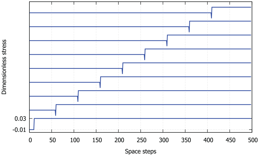
Distribution of shear stress along the bar plotted sequentially for every 50 time steps beginning with that for 50 time steps. The lowest line corresponds to the initial situation.

The corresponding evolution of the shear strain distribution in time is presented in Figure 10.

Figure 10.

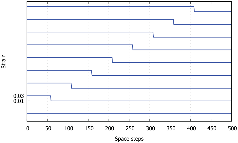
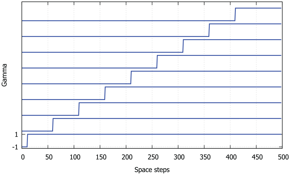
Distribution of shear strain along the bar plotted sequentially for every 50 time steps. The straight line at the bottom shows initial distribution of the shear strain.

It is seen clearly how the variant 1 consecutively occupies the bar that was initially in variant 2. The numerical features of the moving twin boundary treatment are responsible for the spikes in the stress distributions near the twin boundary.

The gradient of the internal variable retains its order parameter nature. Its variation in time repeats the motion of the twin boundary (Figure 11).

Figure 11.

Distribution of gradient of internal variable along the bar plotted sequentially for every 50 time steps. The line at the bottom shows initial distribution of the gradient.

The fast propagation of the twin boundary is confirmed by its position variation as shown in Figure 12. After short time from the initiation of the motion, the velocity of the twin boundary becomes equal to the elastic speed.

Figure 12.

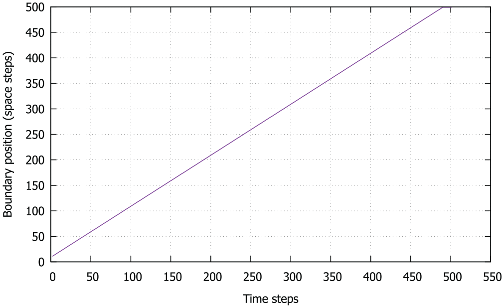
Variation in the twin boundary position in the case of dual internal variable model.

As one can see, numerical simulations using the dual internal variable model demonstrate completely different behavior of twins in comparison with the diffusional growing in the single internal variable case. In the dual internal variable model, the twin boundary propagates along the bar with a high velocity. Such kind of the twin boundary dynamics can be corresponded to the twin tip propagation [6–8].

5. Conclusion

Classical continuum mechanics has no tools to describe equilibrium of twins, not to mention twin boundary motion. The experimental data of twin boundary propagation show a difference of eight orders. To provide additional insight on the motion of twin boundaries, the internal variable model is developed in this paper. The extension of the continuum description of twin boundary motion by internal variables allows for the theoretical distinction between twin slow and fast dynamics. The phase transformation of solids can be categorized into two different types: diffusional and displacive (or diffusionless) phase transformations. The diffusional phase transition is explained using the single internal variable theory, which is the generalization of the phase-field approach. This type of phase transition corresponds to the slow motion of the phase boundary. On the contrary, the displacive phase transition, which involves fast phase boundary dynamics, requires a more general explanation provided by the dual internal variable approach. The dual internal variable model is reduced to the single internal variable model if the corresponding material parameter in the constitutive relation vanishes. Internal variables serve as order parameters indicating the difference in twin variants. Equations of motion are coupled to evolution equations of internal variables. In the uniaxial case, these equations are solved numerically. A slow diffusional motion of a twin boundary is reproduced using a parabolic evolution equation in the case of a single internal variable. In contrast, the dual internal variable approach leads to a hyperbolic evolution equation for the evolution of the primary internal variable and provides fast dynamics of a twin boundary.