Explicit solutions in Cartesian coordinates for an elliptic hole in an infinite elastic plate

Abstract

An explicit analytical solution for an elliptical hole in an infinite elastic plate is derived for uniaxial load from the earliest work on this configuration. This is used along with the biaxial loading case and more recent solutions, available in curvilinear coordinates, to transform the stress fields into Cartesian coordinates along the x and y axes, reducing the curvilinear solutions to simplified short-form expressions of x and y. The present closed-form results are the functions of polynomials of the second and third order of x or y along the x or y axes, respectively, and have the most concise form to the best of the authors’ knowledge. The displacements for plain stress condition are calculated directly from the present stress field expressions, as functions of second-order polynomials of x or y and demonstrate overall consistency. Application of the present stress field and displacements results to special cases, such as a circular hole, a crack, and an elliptical hole in a pressurized cylindrical shell, are shown to agree with published solutions where available.

1. Introduction

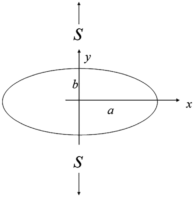
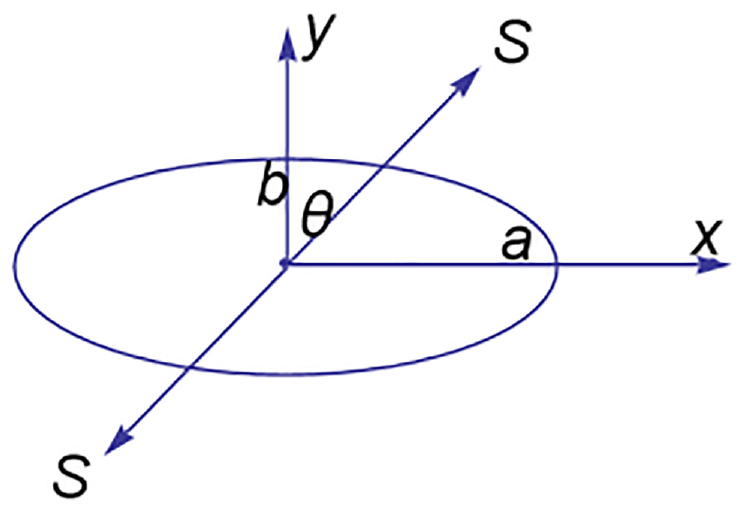
The configuration of an elliptical hole in a plate has been studied for over a century. The solution for stresses due to an elliptical hole in an infinite plate was published by Inglis in 1913 [1]. This included the load cases of remote biaxial uniform stress in all directions, Figure 1, and uniaxial remote stress in any orientation. Inglis derived the explicit stress field over the entire plate, as a function of the curvilinear coordinates α and β per Figure 2, using elliptic coordinates and functions that satisfy Laplace’s equation.

Figure 1.

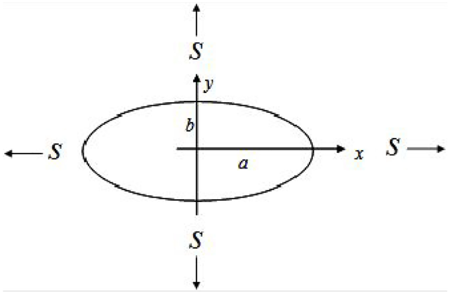
Remote uniform biaxial stress in a plate with an elliptic hole.

Figure 2.

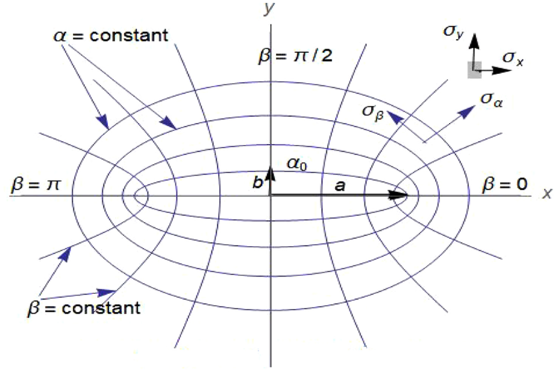
Curvilinear coordinate system.

Multiple related studies of plane elasticity have been published over the years. A comprehensive review of the evolution of and the literature on this topic is provided in the work by Gao [2]. However, it is stated in the work by Gao [2] that at that time, no explicit expressions existed for the stress field due to an elliptical hole in a plate under remote biaxial loading S _x plus S _y simultaneous in x and y directions, such as:

$$S_y=S;\mathrm{Sx}=\gamma S,$$

(1)

where γ is any numerical value; S _y is a remote uniform stress in the y direction, and S _x is a remote uniform stress in the x direction.

A general solution for the stress field and displacements due to loading per equation (1), applied in any orientation, is developed by Gao [2] in terms of the elliptical curvilinear coordinates. Gao [2] is able to present his explicit solutions using a relatively compact notation making them useful for application in the aircraft and pressure vessel industries and others.

From the earlier elliptical hole solution by Inglis to the general solution by Gao, much research on the subject has taken place and has continued to date. A solution for a circular hole in an infinite plate was first developed by Kirsch [3] in 1898 for uniaxial uniform loading. In 1909, Kolosov [4] introduced complex variable approach for solving plane elastic problems. Details of Kirsch [3] and Kolosov [4] are presented in the work by Timoshenko [5]. Solutions for various cases of an elliptical hole in an infinite plate were obtained in the work by Muskhelishvili [6] using Cauchy-type integrals and conformal mapping transformation. Some simplified approaches in complex potential analysis are presented in the work by Stevenson [7] and later used in the work by Gao [2]. The work by Pollard [8] provides the stress field and displacements components in the x and y directions, around an elliptic hole, expressed in terms of curvilinear coordinates. The loadings considered in the work by Pollard [8] are remote axial stress applied in any direction and pressure inside the hole.

With the evolution of computer technology and software development, numerical techniques have been developed and used extensively to solve various configurations. These include finite element modeling (FEM) and boundary element method (BEM) / boundary force method (BFM). FEM results from Klungerbo [9] and BFM results from Badiger and Ramakrishna [10] will be used here for the verification of our results.

A large volume of work in the literature has also been devoted to determining stresses due to various shapes of holes. Savin’s book [11] contains two-dimensional problems of stresses around holes in a plate. It presents the fundamental equations in the theory of plane elasticity and covers a variety of cases of holes in plates under various loadings conditions. These include circular, elliptical, rectangular, and triangular holes in isotropic plates, and circular and elliptical holes in anisotropic plates. Stress concentration around a hole in an infinite plate subjected to a uniform load was investigated in the work by Batista [12] using a modified version of Muskhelishvili’s conformal mapping complex variable method and applied to the holes of various shapes. The method is illustrated by several examples of stress distribution around polygonal holes of a complex geometry using the Schwarz–Christoffel mapping function. A solution for hypotrochoid cutouts in an infinite isotropic plate subjected to in-plane loading is developed by Sharma [13] using Muskhelishvili’s complex variable approach to find stresses and stress intensity factors for different-shaped hypotrochoid holes.

In some contexts, engineers, researchers, and structural scientists would benefit from simplified, concise formulas for the stress fields and displacements due to elliptical holes, expressed in terms of a Cartesian coordinate system: this is precisely the focus of our investigation. Of particular interest is the stress field σ _y (in the y direction) in the material along the x axis of the elliptic hole, see Figure 1, expressed as a function of the x coordinate. This stress field distribution would lend itself for use in stress intensity factor (K_I) estimations using weight functions, (Oore and Burns [14], Oore et al. [15], Livieri and Segala [16] or other) for cracks in 2D or 3D bodies and growing in the x–z plane. Also, such an expression of stress field will be convenient for fatigue damage calculation at small holes (for fasteners, for example) along the x-axis near elliptical openings in panels (such as access holes in aircraft skin). For major loading in the x direction, there would be interest also in σ _x along the y-axis, expressed as a function of the y-coordinate. In addition, the exact stress field expressions (of x or y) can serve conveniently as a benchmark for FEM and BEM modeling of stresses near elliptical holes.

In keeping with the above objective, our present study provides concise expressions for stress distribution fields and displacements along the x-axis and along the y-axis, that are expressed in terms of the Cartesian coordinates. In aerospace and other applications, practical need has prompted us to apply significant effort to transform curvilinear solutions from Inglis [1] and Gao [2] to concise Cartesian form for multiple cases and ensure the validity of our analytically derived results. Despite the lengthy mathematical manipulations involved in intermediary steps, our derivations lead to solutions that are remarkably simple. Our present expressions have the most concise form to date, to the best of our knowledge, and are also consistent with available references, including Kanezaki et al. [17] that used mirror-imaging technique to obtain analytical solutions. In essence, the results in the work by Kanezaki et al. [17] are expressed as functions of fourth- and sixth-order polynomials of x while our present results involve third-order polynomials of x (or y). As will be discussed in the body of this article, a five-tier verification of our results is applied:

1. Numerical /graphic comparison with FEM from Klungerbo [9];

2. Numerical /graphic comparison with boundary force method results from Badiger and Ramakrishna [10];

3. Numerical /graphic comparison with the analytical solution from Gao [2];

4. Numerical comparison with thousands of points along x for various cases from Kanezaki et al. [17];

5. Displacements are calculated directly from the present stress field expressions and are shown to agree with published solutions.

To recapitulate, this study’s focus is on providing expressions for elliptical-hole-induced stress fields and displacements, in simplified concise form and in terms of the Cartesian x or y coordinates, that lend themselves to practical applications. That is, the extensive literature on this topic has been very useful in many situations, but there are certain other specific contexts in which its complexity, either numerical or analytical, has still been a type of limitation. Our work addresses this gap in the literature by providing remarkably simple expressions for the solutions to this problem, that will be highly applicable for individuals working in certain contexts, such as aircraft repairs. We generate concise closed-form solutions in Cartesian coordinates, for multiple cases and loading configurations, including direct and indirect verifications.

We now give a brief overview of how we achieve this: We consider the traction-free condition on the surface of the hole and derive from Inglis [1] the tangential stress field (σ_β) due to remote uniform axial loading S _y  = S and transform it to stresses along x and y in terms of the Cartesian coordinates. As we show based on the general full-field solution of Gao [2] that superposition is applicable (see text following equation (82)), we use the S_y case from Inglis [1] in superposition with the uniform biaxial case (from Inglis [1]) to find solutions for σ_β along x and along y, due to S _x loading. Our solutions for S _x and S _y loadings can be used in superposition to solve for any loading combination per equation (1). We use results from Gao [2] (in superposition with Inglis [1]) to determine the “radial” stress fields (σ _α ) along the x and y axes for loadings in the principal directions, and σ_β along x due to uniaxial load in any direction, and we transform all these into the Cartesian coordinates. We use some of our stress field expressions directly to calculate displacements along x and y, in terms of x or y, showing consistency with published results where available, thereby demonstrating the validity of our results and the application of superposition in these cases. In general, our present results for displacements and stress fields are expressed as polynomial functions of the coordinates x or y and the elliptic hole dimensions a and b. In some cases, these are normalized. The solutions are derived here for the positive sides of the x and y axes, and it is later discussed how to apply them to the negative sides of the x and y axes with a trivial modification.

It is interesting to note that in 1921, Griffith [18] used Inglis’ solution to evaluate, for the first time, the energy release rate due to crack extension. However, the first solution for the stress field due to a crack was obtained in the work by Westergaard [19] in 1939, unrelated to Inglis’ work. It will be shown here that our solution, as derived from Inglis, also provides the stress field due to a crack, when we let the ellipse minor axis b→ 0. It is interesting that the crack stress field solution was “hidden” in Inglis’ elliptic hole solution [1] for decades, before it was developed independently in Westergaard [19] and unrelated to Inglis [1].

2. Analysis

2.1. Elliptical hole in a plate under remote biaxial stress uniform in all directions—stresses and displacements along the x-axis in Cartesian coordinates

The configuration and loading for this case, Sy = S _x  = S, are depicted in Figure 1. The curvilinear coordinate system selected here is explained in the work by Timoshenko [5] but the coordinate designations here are α and β per the original work in Inglis [1] as shown in Figure 2.

The coordinates α and β are related to the Cartesian coordinate system (x; y) via the equations:

$$x=c\cosh \left(\alpha \right)\cos \left(\beta \right),$$

(2)

$$y=c\sinh \left(\alpha \right)\sin \left(\beta \right),$$

(3)

where c is a constant. For α = constants, equations (2) and (3) define a family of ellipses and for β = constants, they define a family of hyperbolas as shown in Figure 2.

Designating by α₀, the coordinate of the elliptic hole with major and minor semi axes a and b, respectively, see Figure 2, stems from equations (2) and (3), for β = 0 and β = π/2, respectively, that:

$$a=c\cosh \left({\alpha }_0\right),b=c\sinh ({\alpha }_0),{\alpha }_0=\tan {\mathrm{h}}^{-1}(b/a)=\cos {\mathrm{h}}^{-1}(a/c),$$

(4)

from which we get $c=\sqrt{a^2-b^2}$ , that is, the focal distance of the elliptical hole, which is the same for all the α coordinates.

The tangential component σ_β (tangential to α = constant and normal to β = constant) of the stress field due to a uniform biaxial stress S is given in [1] by:

$${\sigma }_{\beta }=\frac{S\sinh 2\alpha (\cosh 2\alpha +\cosh 2{\alpha }_0-2\cos 2\beta )}{{(\cosh 2\alpha -\cos 2\beta )}^2}.$$

(5)

Considering the stress σ_y along x (σ_y =σ_{β|β = 0}), we substitute β = 0 in equation (5) giving:

$${\sigma }_y=\frac{S\sinh 2\alpha (\cosh 2\alpha +\cosh 2{\alpha }_0-2)}{{(\cosh 2\alpha -1)}^2}.$$

(6)

We transform equation (6) from elliptic curvilinear into the Cartesian coordinate system along x with the transformation:

$$\alpha =\cos {\mathrm{h}}^{-1}\frac{x}{c},$$

(7)

which results from substituting β = 0 in equation (2).

Substituting α₀ from equation (4) and α from equation (7) in equation (6) gives:

$${\sigma }_y=\frac{S\sinh (2\cos {\mathrm{h}}^{-1}\frac{x}{c})(\cosh (2\tan {\mathrm{h}}^{-1}\frac{b}{a})+\cosh (2\cos {\mathrm{h}}^{-1}\frac{x}{c})-2)}{{[\cosh (2\cos {\mathrm{h}}^{-1}\frac{x}{c})-1]}^2}.$$

(8)

We substitute $c=\sqrt{a^2-b^2}$ in equation (8) and apply hyperbolic function expansions and mathematical manipulations and simplifications giving:

$${\sigma }_y=\frac{Sx(x^2-a^2+2b^2)}{{(x^2-a^2+b^2)}^{3/2}}.$$

(9)

We note that in the simplification of equation (8), and of many other long equations in the following sections, despite access to software, such as Mathematica or Maple, the manipulations are not trivial. In some cases, the first expansion results in a sum of 500 terms in which each term is by itself a product of 15 terms and the system cannot automatically simplify all this much further. Thus, when at various points in this paper, we say that we have “applied mathematical manipulations” to simplify these equations, what this means is that we

1. Manually rearrange and substitute various terms by inspection;

2. Apply computational mathematical approaches to further simplify the resulting expressions;

3. Continue to iterate the above Steps (1) and (2) until we arrive at our final results in all of these cases.

The simple form of equation (9) provides the normal stress σ _y ahead of the hole along the x-axis in terms of the remote biaxial stress S, the coordinate x and the major and minor semi axes of the ellipse a and b, respectively. To the best of our knowledge, this is the most concise closed-form solution to date for this case. It is interesting to note, as will be shown later, that equation (9) provides the proper results along x also for b/a > 1.

When $x\to \infty$ in equation (9) then σ _y →S as expected infinitely remote from the hole.

Substituting x = a in equation (9) to find the stress at the tip of the axis a, on the edge of the elliptical hole, gives:

$${\sigma }_y=\frac{2aS}{b},$$

(10)

which is the known solution for this case. Substituting b = a in equation (9) gives:

$${\sigma }_y=S(\frac{a^2}{x^2}+1),$$

(11)

showing that equation (9) converges to the known solution for the stress field due to a circular hole in a plate subjected to remote biaxial uniform stress S. To explore how equation (9) handles elliptical hole with an extreme aspect ratio, we substitute b = 0 in equation (9) which degenerates the elliptical hole into a crack of length 2a giving:

$${\sigma }_y=\frac{Sx}{\sqrt{x^2-a^2}}.$$

(12)

We introduce a local coordinate system r whose origin is at the tip of the crack by substituting

x = a + r in equation (12) giving:

$${\sigma }_y=\frac{S(a+r)}{\sqrt{r(2a+r)}}.$$

(13)

For the stress field near the tip of the crack, we calculate the asymptotic limit of equation (13)

when r→0 giving:

$${\sigma }_y=\frac{\sqrt{a}s}{\sqrt{2}\sqrt{r}}.$$

(14)

Equation (14) is identical to the well-known first term of the crack-tip stress field solution for this case. Hence, equation (9) gives the same stress intensity factor K_I as the published classical solution for a crack. By expansion of equation (13) to Taylor series we obtain,

$${\sigma }_y=\frac{\sqrt{a}S}{\sqrt{2}\sqrt{r}}+\frac{3\sqrt{r}S}{4\sqrt{2}\sqrt{a}}-\frac{5r^{3/2}S}{32\left(\sqrt{2}{a}^{3/2}\right)}+\frac{7r^{5/2}S}{128\sqrt{2}{a}^{5/2}}+O\left(r^{7/2}\right)+\dots$$

(15)

which contains the same terms as the published solution for the stress field near and away from the crack tip. Equation (15) demonstrates the validity of equation (9) for extreme geometry.

We normalize equation (9) using the following substitutions: σ _n  =σ _y /S; χ = x/a; λ = b/a giving:

$${\sigma }_n=\frac{\chi (2{\lambda }^2+{\chi }^2-1)}{{({\lambda }^2+{\chi }^2-1)}^{3/2}}.$$

(16)

Plots of normalized stress per equation (16) are shown in Figures 3 and 4 over different χ intervals. Note that the curves cross each other. Since the area under each curve should include the same load carried originally along the ellipse’s major axis prior to the existence of the hole, the curves that start higher need to cross those which start lower to maintain the same total area under the curve.

Figure 3.

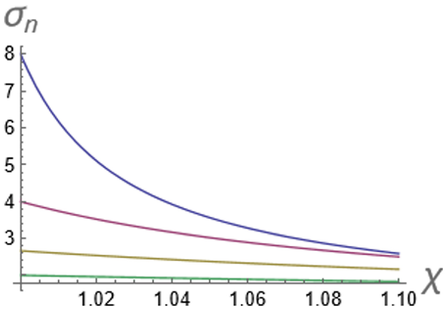
Normalized stress σ _y along χ for λ = 0.25, 0.5, 0.75, and 1.0 due to uniform biaxial load.

Figure 4.

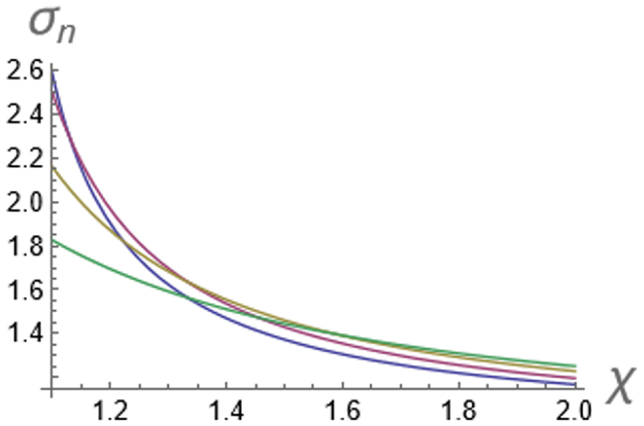
Normalized stress σ _y along χ for λ = 0.25, 0.5, 0.75, and 1.0 due to uniform biaxial load.

The stress field σ _yp due to a case of internal pressure loading S, acting uniformly on the surface of the hole, can be obtained with superposition by subtracting S from the solution for the biaxial all-round remote uniform stress case. This gives σ _yp  = equation (9)−S, or, in normalized form, σ _pn  =equation (16)−1 along the x axis.

To further validate the stress field per equation (16), we calculate the area under its curve but above a unit stress horizontal line (σ _n  =1), from the edge of the hole at χ = 1 to a given distance z, giving a force A:

$$A={\int }_1^z({\sigma }_n-1)\mathbb{d}\chi =\frac{z^2-1-z\sqrt{{\lambda }^2+z^2-1}}{\sqrt{{\lambda }^2+z^2-1}}+1.$$

(17)

The total force A across half the infinite plate should be equal to the original load F =a S carried by the material in the region a of the hole prior to the existence of the hole. In normalized terms per above, this would be F _n given by:

$$F_n=\frac{F}{aS}=\frac{aS}{aS}=1.$$

(18)

To calculate the total load A from equation (17), we take z to infinity to cover the right half of the infinite plate giving:

$$A_{z\to \infty }=\underset{z\to \infty }{\mathrm{limit}}(\frac{z^2-1-z\sqrt{{\lambda }^2+z^2-1}}{\sqrt{{\lambda }^2+z^2-1}}+1)=1.$$

(19)

Hence, equations (17) and (19) give a result identical to the required value per equation (18) and thus, we conclude that the stress field per equations (16) and (9) satisfies the basic loading equilibrium.

The radial component σ _α of the stress field due to biaxial stress S is given in the work by Inglis [1]:

$${\sigma }_{\alpha }=\frac{S\left\{\sinh 2\alpha [\cosh 2\alpha -\cosh 2{\alpha }_0]\right\}}{{(\cosh 2\alpha -\cos 2\alpha )}^2}.$$

(20)

Considering the stress σ _x along x (σ _x  =σ_{α|β = 0}), we substitute β = 0 and α₀ per equation (4) in equation (20) giving:

$${\mathrm{\sigma }}_x=\frac{S\sinh 2\alpha [\cosh 2\alpha -\cosh \left(2\tan {\mathrm{h}}^{-1}\frac{b}{a}\right)]}{{(\cosh 2\alpha -1)}^2}.$$

(21)

We transform equation (21) from elliptic curvilinear coordinates into the Cartesian coordinate system with the transformation per equation (7) giving:

$${\sigma }_x=\frac{S\sinh \left(2\cos {\mathrm{h}}^{-1}\frac{x}{c}\right)[\cosh \left(2\cos {\mathrm{h}}^{-1}\frac{x}{c}\right)-\cosh \left(2\tan {\mathrm{h}}^{-1}\frac{b}{a}\right)]}{{[\cosh \left(2\cos {\mathrm{h}}^{-1}\frac{x}{c}\right)-1]}^2}.$$

(22)

Using mathematical manipulations and simplification on equation (22) gives:

$${\sigma }_x=\frac{Sx(x^2-a^2)}{{(x^2-a^2+b^2)}^{3/2}}.$$

(23)

It is noted that the stress field σ _xp due to a case of internal pressure loading S, acting uniformly on the surface of the hole, can be obtained with superposition by subtracting S from the solution for the biaxial all-round remote uniform stress case. This gives σ _xp  = equation (23)−S along the x-axis.

When x→∞ in equation (23), then σ _x →S as is the case infinitely remote from the hole.

Substituting x = a in equation (23) to find the stress at the tip of the major axis, on the edge of the elliptical hole gives σ _x  = 0 which is indeed the normal stress state on the surface of the hole.

Substituting b = a in equation (23) gives:

$${\sigma }_x=S(1-\frac{a^2}{x^2}),$$

(24)

showing that equation (23) converges to the known solution of the radial stress field due to a circular hole in a plate subjected to remote biaxial uniform stress. To explore how equation (23) handles an elliptical hole with an extreme aspect ratio, we substitute b = 0 in equation (23) which degenerates the elliptical hole into a crack of length 2a giving:

$${\sigma }_x=\frac{Sx}{\sqrt{x^2-a^2}},$$

(25)

which is identical to the published crack solution for the σ _x component of the stress field along x.

The displacements in the y-direction along the x-axis are nil due to symmetry. The displacements δ_x in the x-direction along the x-axis can be determined by transforming published solutions in curvilinear coordinates into Cartesian coordinates using the transformation per equations (4) and (7), or calculated directly using σ _x and σ _y from equations (23) and (9), respectively. Here, we will use first the latter approach, the results of which can serve to further demonstrate the validity of equations (23) and (9).

The displacement δ_X of any point at position X on the x-axis can be shown to be given by:

$${\delta }_X={\delta }_R-{\delta }_{\mathrm{XR}},$$

(26)

where δ _R is the displacement of a remote point at position R on the x-axis and δ _XR is the elongation of the material between X and R. We note that the strain ε _x along the x-axis is given for plain stress condition by:

$${\epsilon }_x=\frac{{\sigma }_x-\nu {\sigma }_y}{E},$$

(27)

and that:

$${\delta }_{\mathrm{XR}}={\int }_X^R{\epsilon }_x\mathbb{d}x,$$

(28)

At a very remote point where R→∞, the local effect of the hole diminishes and δ _R is given by:

$${\delta }_{R\to \infty }=\frac{S(1-\nu )}{E}R.$$

(29)

We substitute equations (23) and (9) in equation (27) and then equation (27) in equation (28), integrate per equation (28) and substitute it and equation (29) in equation (26).

The displacement δ _X along x can now be calculated by letting R go to infinity in equation (26) giving:

$${\delta }_X=\underset{R\to \infty }{\mathrm{limit}}({\delta }_R-{\delta }_{\mathrm{XR}})=\frac{S[(1-\nu )(X^2-a^2)+2b^2]}{E\sqrt{X^2-a^2+b^2}}.$$

(30)

Note that when X→∞ in equation (30), then ${\delta }_X\to \frac{(1-\nu )\mathrm{SX}}{E}$ as expected at a point infinitely far from a hole in a plate under remote uniform biaxial uniform stress.

When X = a in equation (30), then ${\delta }_X=\frac{2\mathrm{bS}}{E}$ which is the same as the result presented in Griffith [18] at the tip of the major axis of a hole in a plate under remote biaxial uniform stress.

When we substitute b = a in equation (30), we get the displacement expression due to a circular hole as:

$${\delta }_X=\frac{S[X^2(1-\nu )+a^2(1+\nu )]}{EX}.$$

(31)

When we substitute X = a in equation (31), then δ _X  =  $\frac{2aS}{E}$ which agrees with the known displacement on the edge of a circular hole for this loading.

To further validate equation (30) and the procedure used to derive it, we will derive in the following displacements for this case of remote biaxial uniform stress using results from the work by Timoshenko [5] p.190 which can be represented as:

$$2G({\delta }_x+\mathbb{i}{\mathrm{\delta }}_y)=\frac{(3-\nu )}{2(\nu +1)}cS\sinh (\alpha +\mathbb{i}\beta )-\frac{1}{2}cS\cosh (\alpha +\mathbb{i}\beta )\coth (\alpha -\mathbb{i}\beta )+\frac{\mathrm{c}S\cosh 2{\alpha }_0}{2\sinh (\alpha -\mathbb{i}\beta )},$$

(32)

where δ _x and δ _y are the displacements in the x- and y-directions, respectively, and G is the elastic shear modulus.

To consider displacements along x, we substitute β = 0 and the expression of G = $\frac{(1+\nu )E}{2}$ in equation (32) giving:

$$({\delta }_x+\mathbb{i}{\mathrm{\delta }}_y)=\frac{(\nu +1)}{2E}\{cS\mathrm{csch}\alpha \cosh 2{\alpha }_0+\frac{c(3-\nu )S\sinh \alpha }{(\nu +1)}-cS\cosh \alpha \coth \alpha \}.$$

(33)

From equation (33), we see that δ _y  =0 as we also expect due to symmetry along x. Substituting in equation (33) that $c=\sqrt{a^2-b^2}$ and the expressions of α₀ and α from equation (4) and equation (7) give for δ _x after mathematical manipulations the same expression as equation (30). This validates equation (30) and also demonstrates the validity of the stress field equations, equation (9) and equation (23), that were used here to derive equation (30).

2.2. Elliptical hole in a plate under remote uniaxial uniform load—stress and displacements along the x-axis in Cartesian coordinates

The configuration and loading for this case, S _y  = S, are depicted in Figure 5.

Figure 5.

Remote uniaxial uniform stress applied to an infinite plate with an elliptical hole.

We derive the stress field for this case from the work by Inglis [1] and obtain the tangential component σ_β of the stress as:

$$\begin{array}{c}\multicolumn{1}{c}{{\sigma }_{\beta }=\frac{S}{{(\cosh 2\alpha -\cos 2\beta )}^2}}\\ \multicolumn{1}{c}{\{(-\frac{{\mathbb{e}}^{2{\alpha }_0}}{8}-\frac{1}{16})(-8{\mathrm{e}}^{-2\alpha }\cos 2\beta +2{\mathbb{e}}^{-4\alpha }+2\cos 4\beta +4)+\frac{1}{16}(-8{\mathbb{e}}^{2\alpha }\cos 2\beta +2{\mathbb{e}}^{4\alpha }+2\cos 4\beta +4)}\\ \multicolumn{1}{c}{+\frac{1}{8}{\mathbb{e}}^{4{\alpha }_0}(({\mathbb{e}}^{-4\alpha }+3)\cos \left(2\beta \right)-{\mathbb{e}}^{-2\alpha }\cos 4\beta -3{\mathbb{e}}^{-2\alpha })+\frac{1}{8}(({\mathbb{e}}^{4\alpha }+3)\cos 2\beta -{\mathbb{e}}^{2\alpha }\cos 4\beta -3{\mathbb{e}}^{2\alpha })}\\ \multicolumn{1}{c}{+\frac{1}{4}({\mathbb{e}}^{2\alpha }-{\mathbb{e}}^{-2\alpha })(\cosh 2{\alpha }_0+1)\}.}\end{array}$$

(34)

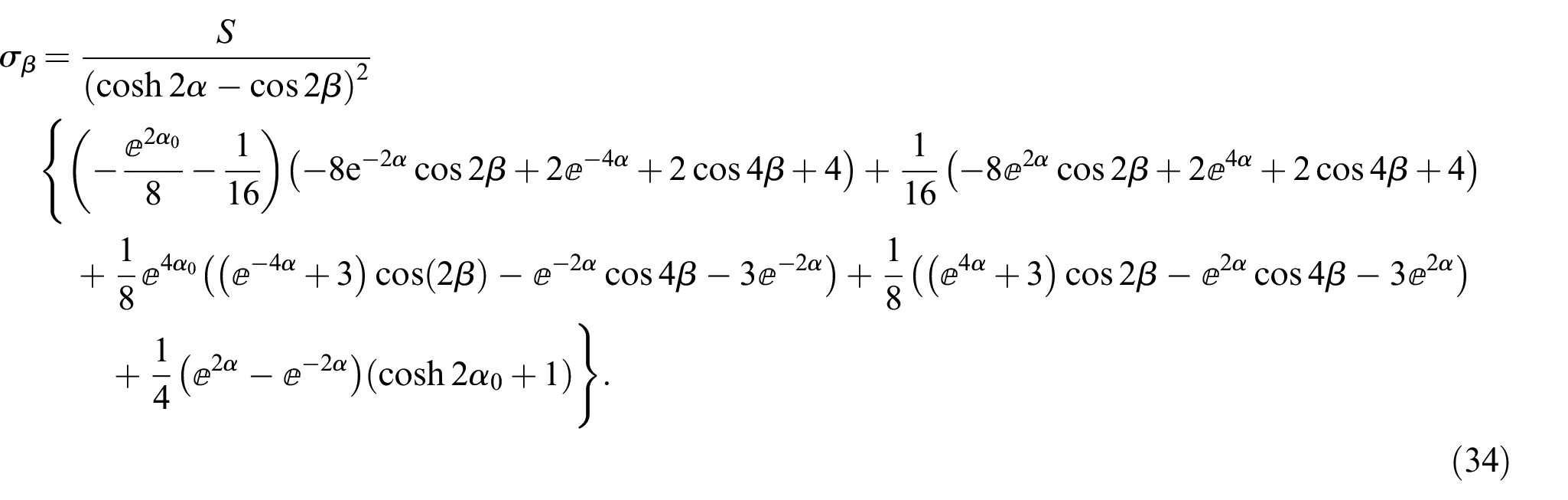
Considering the stress σ _y along x, (σ _y  =σ_{β|β = 0}), we substitute β = 0 in equation (34) giving:

$$\begin{array}{c}\multicolumn{1}{c}{{\sigma }_y=\frac{S}{{(\cosh \left(2\alpha \right)-1)}^2}[\frac{1}{8}{\mathbb{e}}^{4{\alpha }_0}({\mathbb{e}}^{-4\alpha }-4{\mathbb{e}}^{-2\alpha }+3)+(-\frac{{\mathbb{e}}^{2{\alpha }_0}}{8}-\frac{1}{16})(2{\mathbb{e}}^{-4\alpha }-8{\mathbb{e}}^{-2\alpha }+6)}\\ \multicolumn{1}{c}{+\frac{1}{8}(-4{\mathbb{e}}^{2\alpha }+{\mathbb{e}}^{4\alpha }+3)+\frac{1}{16}(-8{\mathbb{e}}^{2\alpha }+2{\mathbb{e}}^{4\alpha }+6)+\frac{1}{4}({\mathbb{e}}^{2\alpha }-{\mathbb{e}}^{-2\alpha })(\cosh 2{\alpha }_0+1)]}\\ \multicolumn{1}{c}{(\cosh \left(2{\alpha }_0\right)+1)))}\end{array}$$

(35)

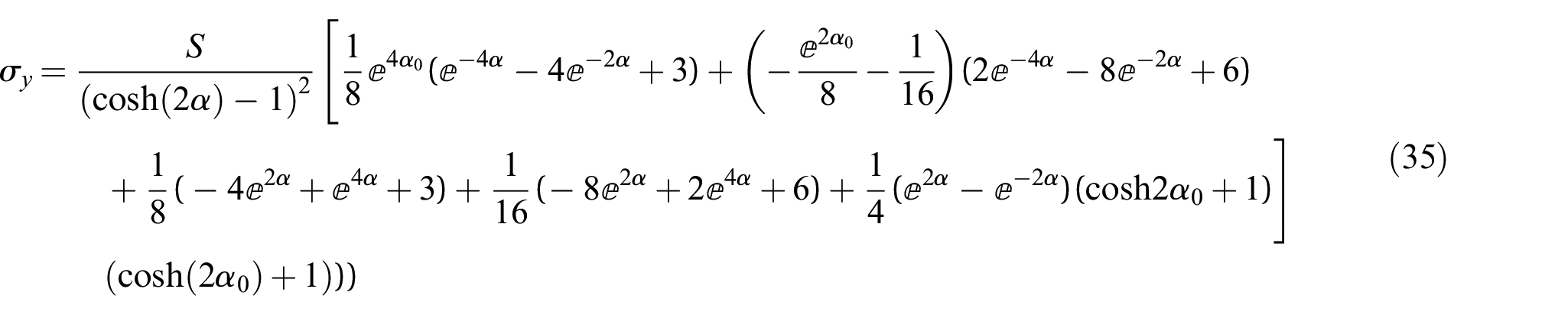
We transform equation (35) from elliptic curvilinear coordinates into the Cartesian coordinate system with the transformation per equations (4) and (7) giving:

$$\begin{array}{c}\multicolumn{1}{c}{{\sigma }_y=\frac{S}{{(\cosh \left(2\cos {\mathrm{h}}^{-1}\left(\frac{x}{c}\right)\right)-1)}^2}\{\frac{1}{8}{\mathbb{e}}^{4\tan {\mathrm{h}}^{-1}\left(\frac{b}{a}\right)}({\mathbb{e}}^{-4\cos {\mathrm{h}}^{-1}\left(\frac{x}{c}\right)}-4{\mathbb{e}}^{-2\cos {\mathrm{h}}^{-1}\left(\frac{x}{c}\right)}+3)}\\ \multicolumn{1}{c}{+\frac{1}{4}({\mathbb{e}}^{2\cos {\mathrm{h}}^{-1}\left(\frac{x}{c}\right)}-{\mathbb{e}}^{-2\cos {\mathrm{h}}^{-1}\left(\frac{x}{c}\right)})(\cosh \left(2\tan {\mathrm{h}}^{-1}\left(\frac{b}{a}\right)\right)+1)+(2{\mathbb{e}}^{-4\cos {\mathrm{h}}^{-1}\left(\frac{x}{c}\right)}-8{\mathbb{e}}^{-2\cos {\mathrm{h}}^{-1}\left(\frac{x}{c}\right)}+6)}\\ \multicolumn{1}{c}{(-\frac{1}{8}{\mathbb{e}}^{2\tan {\mathrm{h}}^{-1}\left(\frac{b}{a}\right)}-\frac{1}{16})-\frac{1}{8}(4{\mathbb{e}}^{2\cos {\mathrm{h}}^{-1}\left(\frac{x}{c}\right)}-{\mathbb{e}}^{4\cos {\mathrm{h}}^{-1}\left(\frac{x}{c}\right)}-3)-\frac{1}{16}(8{\mathbb{e}}^{2\cos {\mathrm{h}}^{-1}\left(\frac{x}{c}\right)}-2{\mathbb{e}}^{4\cos {\mathrm{h}}^{-1}\left(\frac{x}{c}\right)}-6)\}}\end{array}$$

(36)

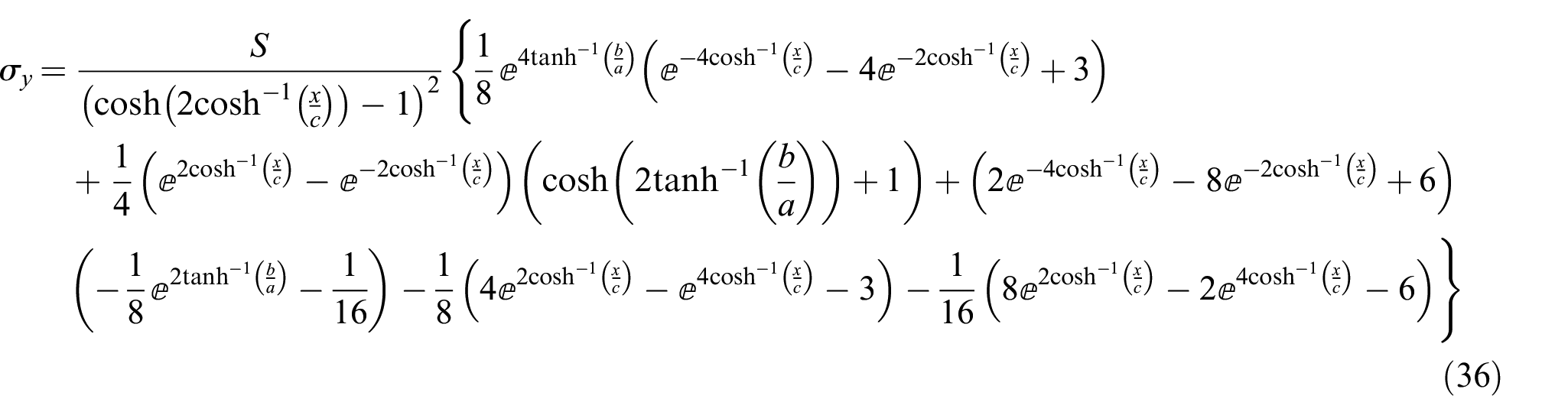
Substituting in equation (36) that $c=\sqrt{a^2-b^2}$ and using lengthy mathematical manipulations, we simplify equation (36) to obtain:

$${\sigma }_y=\frac{b^{2}S}{{(a-b)}^2}-\frac{Sxa[a^3-2a^{2}b-2a{b}^2+3b^3-x^2(a-2b)]}{{(a-b)}^2{(x^2-a^2+b^2)}^{3/2}}.$$

(37)

The simplified form of equation (37) provides the σ _y stress field along x in terms of the remote stress S (=S_y), the coordinate x, and the major and minor semi axes of the ellipse a and b, respectively, for the first time in this form, to the best of our knowledge. It is interesting to note, as will be shown later, that equation (37) provides the proper result also for b/a > 1. Substituting x = a in equation (37) gives the stress at the tip of the major axis on the surface of the elliptic hole as:

$${\sigma }_y=S(\frac{2a}{b}+1).$$

(38)

Equation (38) is identical to the published stress solution at the edge of an elliptical hole in an infinite plate subjected to uniaxial load S _y  = S. Substituting b = a in equation (38) gives the known stress, 3 S, for a circular hole. By some manipulation of equation (37) and substitution of b→a, we obtain:

$${\sigma }_y=\frac{1}{2}S(\frac{3a^4}{x^4}+\frac{a^2}{x^2}+2),$$

(39)

which is identical to the published stress field due to a circular hole in an infinite plate under such loading.

To explore how equation (37) handles an elliptical hole with an extreme aspect ratio, we substitute b = 0 in equation (37) (which degenerates the elliptical hole into a crack of length 2a) giving σ _y  = (S x)/ $\sqrt{x^2-a^2}$ , that is, the same result as in the work by Westergaard [19] and also equation (12) through equation (15). This shows that equation (37) indeed provides the known singularity and stress intensity factor when modeling a crack.

We normalize equation (37) using the following substitutions: σ _yn  =σ_y/S; χ = x/a; λ = b/a giving:

$${\sigma }_{\mathrm{yn}}=\frac{{\lambda }^2}{{(1-\lambda )}^2}(1-\frac{\chi (1-2\lambda -2{\lambda }^2+3{\lambda }^3)+{\chi }^3(2\lambda -1)}{{\lambda }^2{({\chi }^2-1+{\lambda }^2)}^{3/2}}).$$

(40)

To the best of our knowledge, equation (40) is the most concise closed-form solution to date for this case of S _y  = S. While equation (40) is significantly more concise than the corresponding closed-form solution in the work by Kanezaki et al. [17] for this case, they both converge to the same expression at the tip of the major axis of the hole.

To numerically validate our results, we compare equation (40) with the corresponding equation (13) in the work by Kanezaki et al. [17] on a set of points for different values of λ and χ. Specifically, we use a set of 1200 uniformly spaced points in the intervals 0.1 ≤ λ ≤ 0.9 and 1 ≤ χ ≤ 8. We will refer to this set of points as our validation set . The numerical comparison of equation (40) with equation (13) in the work by Kanezaki et al. [17] gave identical results, within 18 digits for all 1200 points in our validation set .

Plots of normalized stress per equation (40) are shown in Figures 6 and 7 over different χ intervals. Note that the curves cross each other for the same reason explained previously regarding equation (16).

Figure 6.

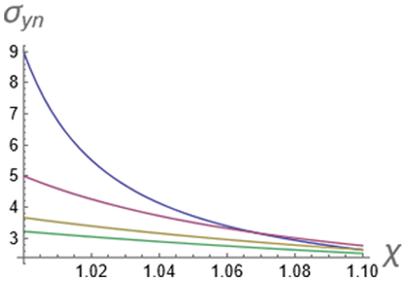
Normalized stress σ _y along χ for λ = 0.25, 0.5, 0.75, and 0.9 due to axial load in the y-direction.

Figure 7.

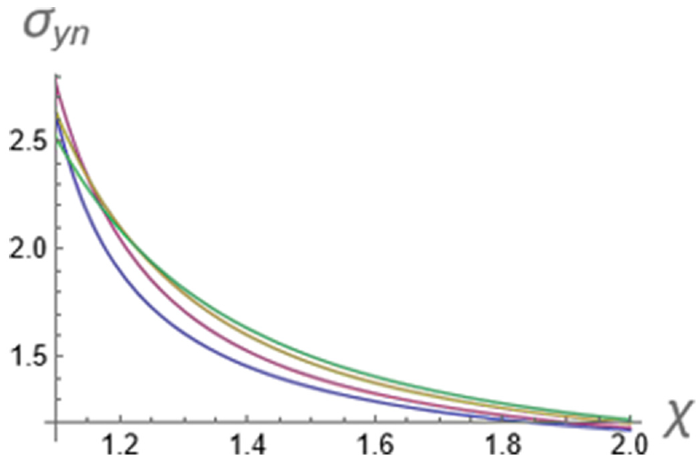
Normalized stress σ _y along χ for λ = 0.25, 0.5, 0.75, and 1.0 due to axial load in the y-direction.

To further validate the stress field per equation (40), we calculate the area under its curve but above a unit stress horizontal line (σ _n  =1), from the edge of the hole at χ = 1 to a given distance z giving a force A:

$$A={\int }_1^z({\sigma }_{\mathrm{yn}}-1)\mathbb{d}\chi ==\frac{-{\lambda }^3+(1-2\lambda )z^2+{\lambda }^2\sqrt{{\lambda }^2+(z+2)z}+(2\lambda -1)z(\sqrt{{\lambda }^2+(z+2)z}-2)}{{(\lambda -1)}^2\sqrt{{\lambda }^2+(z+2)z}}.$$

(41)

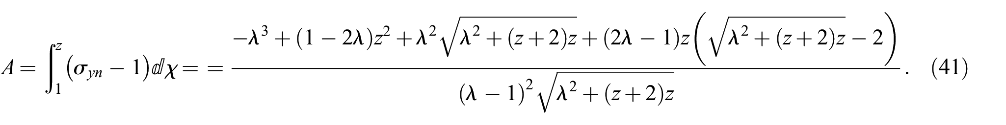
The total force A across half the infinite plate should be equal to the original load F carried by the material in the region a of the hole prior to the existence of the hole, and as shown in equation (18) in normalized terms per above F _n  =1.

To calculate the total load A from equation (41), we take Z to infinity to cover the right half of the infinite plate giving:

$$A_{z\to \infty }=\underset{z\to \infty }{\mathrm{limit}}\left(\frac{(1-2\lambda )z^2-{\lambda }^3+{\lambda }^2\sqrt{{\lambda }^2+z(z+2)}+(2\lambda -1)z(\sqrt{{\lambda }^2+z(z+2)}-2)}{{(\lambda -1)}^2\sqrt{{\lambda }^2+z(z+2)}}\right)=1.$$

(42)

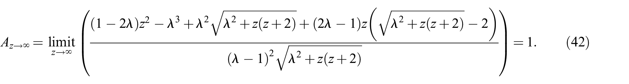
The result of equation (42) is identical to the value of F _n  = 1 (as equation (18)) and thus shows that the stress field per equation (40) (and equation (37)) satisfies the global loading equilibrium.

The normalized stress field σ_yn (in the y-direction) along x due to a remote uniaxial uniform stress in the x-direction, S _x  = S, can be obtained by superposition of the two corresponding previous loading cases (biaxial-uniaxial) as:

$${\sigma }_{\mathrm{yn}}={\sigma }_{\mathrm{yn}}\left[\mathrm{Eq}\left(16\right)\right]-{\sigma }_{\mathrm{yn}}\left[\mathrm{Eq}\left(40\right)\right].$$

(43)

Substituting equations (16) and (40) in equation (43) gives after some mathematical manipulations:

$${\sigma }_{\mathrm{yn}}=\frac{{\lambda }^2}{{(1-\lambda )}^2}(\frac{{\chi }^3-(1-2{\lambda }^2+\lambda )\chi }{{({\lambda }^2+{\chi }^2-1)}^{3/2}}-1).$$

(44)

A numerical comparison of equation (44) with the corresponding equation (18) in the work by Kanezaki et al. [17] gave identical numerical results, within 18 digits, for all 1200 points in our validation set .

Plots of equation (44) are shown in Figure 8. For each curve, the total areas above and below the χ axis are equal so the net force on the total plate section is zero as is the remote stress in the y-direction for this load case.

Figure 8.

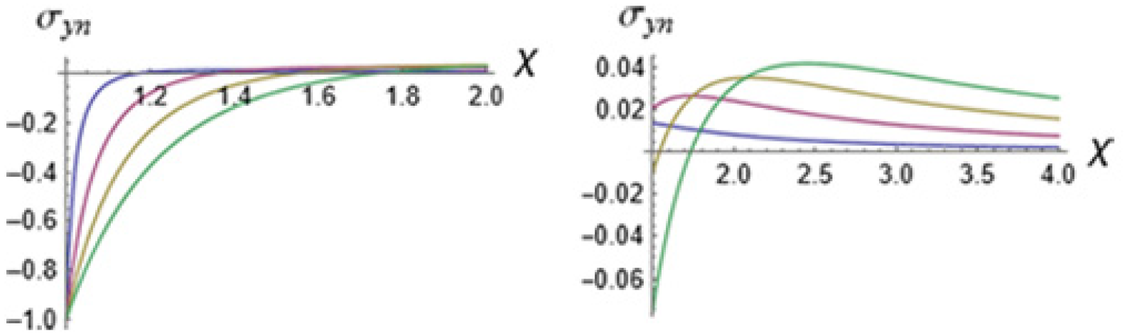
Normalized stress σ _y along x for λ = 0.25, 0.5, 0.75, and 1.0 due to uniaxial load in the x-direction.

Equations (40) and (44) can be used in superposition per equation (1) to produce the elastic stress field along x for any simultaneous combination of remote stresses S _y  = S, and S _x  = γS acting in the y- and x-directions, respectively.

2.3. Example

Consider the case of a pressurized cylindrical shell of thin wall with an elliptical hole with its major axis in the hoop direction designated by x. This can represent an aircraft fuselage or a pressure vessel. In this case γ = 2, the longitudinal stress due to pressure is S and we consider the longitudinal stress σ _y along the x-axis (β = 0). Using superposition, we write σ_yn = Equation (40) +2 equation (44)) which gives after mathematical manipulations:

$${\sigma }_{\mathrm{yn}}=\frac{{\lambda }^2}{{(1-\lambda )}^2}-2+\frac{(2\lambda -1-5{\lambda }^3+4{\lambda }^4)\chi +(1-2\lambda +2{\lambda }^2){\chi }^3}{{(1-\lambda )}^2{({\chi }^2-1+{\lambda }^2)}^{3/2}}.$$

(45)

Substituting in equation (45), a specific elliptic hole geometry of λ = b/a = 1/2, and χ = 1 to consider the tip of the major axis of the hole gives σ _yn  = 3 S which is identical to the result in the work by Gao [2] from the general solution which provides the explicit value at the edge of the hole for this configuration and loading. Equation (45) gives a stress field that could be used for fatigue and cracking analysis along the x (major) axis of the elliptic hole which sustains higher tensile stresses than the minor axis due to the larger stress concentration [end of example].

To determine the radial stress σ _x along the x-axis (σ _x  = σ_{α|β = 0}) due to a remote uniaxial stress in the y-direction, S _y  = S, we use the results from the work by Gao [2] to calculate σ _x  + σ _y along the x-axis due to a uniform uniaxial stress S in the y-direction using equations (29) and (30) from Gao [2] giving:

$${\sigma }_x+{\sigma }_y=\frac{\mathrm{S}({\mathbb{e}}^{2{\alpha }_0}+1)\sinh 2\alpha }{2(\cos {\mathrm{h}}^2\alpha -1)}-S{\mathbb{e}}^{2{\alpha }_0}.$$

(46)

Substituting equation (4) and equation (7) in equation (46) and using mathematical manipulations, we get:

$${\sigma }_x+{\sigma }_y=\frac{2Sax}{(a-b)\sqrt{x^2-a^2+b^2}}-\frac{S(a+b)}{a-b}.$$

(47)

We write σ _x  = (σ _x  + σ _y )-σ _y  = equation (47)−equation (37) which gives after mathematical manipulations:

$${\sigma }_x=\frac{a^{2}S}{{(a-b)}^2}(\frac{x(x^2-a^2+\frac{b}{a}{b}^2)}{{(x^2-a^2+b^2)}^{3/2}}-1).$$

(48)

Equation (48) provides the distribution of the radial stress field σ _x along the x-axis (σ _x  =σ_{α|β = 0}) due to remote uniaxial stress in the y-direction, S _y  = S. Substituting x = a or x = ∞ in equation (48) gives 0, as expected on the surface of the hole and far away from it, for this uniaxial loading. For b→a, equation (48) gives the same result as the known solution for a circular hole for this loading.

While equation (48) is again more concise than the corresponding closed-form solution in the work by Kanezaki et al. [17] for this case, they both converge to the same expression at the tip of the major axis of the hole. Moreover, a numerical comparison of equation (48) with the corresponding equation (12) in the work by Kanezaki et al. [17], for several values of a, b and x, gave identical results within 18 digits for all 1200 points in the validation set .

The displacements along the x-axis due to the uniaxial load S in the y-direction, S _y  = S, are calculated directly using σ _x and σ _y from equations (48) and (37), respectively. The results may serve to further demonstrate the validity of equations (37) and (48). We follow the procedure we used previously, equation (26) through equation (29) with the only difference that now σ _y and σ _x are taken from equations (37) and (48), respectively, and equation (29) is replaced with:

$${\delta }_R=\frac{-\nu S}{E}R,$$

(49)

as the displacement at infinitely remote point R on the x-axis.

Using equation (49), the displacement δ _X is calculated by letting R go to infinity in equation (26) giving:

$${\delta }_X=\underset{R\to \infty }{\mathrm{limit}}({\delta }_R-{\delta }_{\mathrm{XR}})=\frac{Sa{X}^2(a(1-\nu )+2b\nu )+Sa(2a{b}^2-(a^3+b^3)(1-\nu )-2a^{2}b\nu )}{{(a-b)}^{2}E\sqrt{X^2-a^2+b^2}}-\frac{SX(a^2+b^2\nu )}{{(a-b)}^{2}E}.$$

(50)

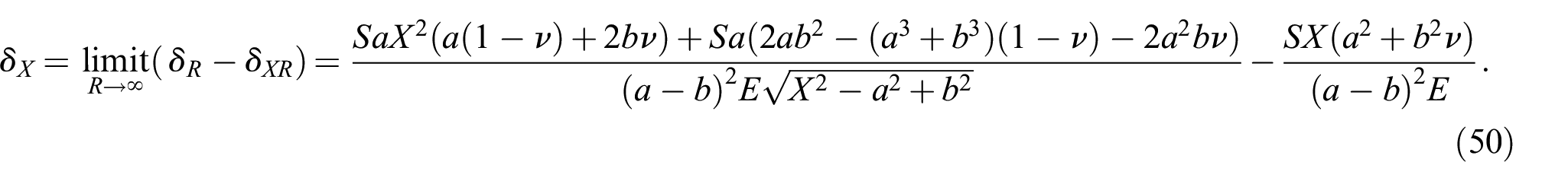
When X→∞ in equation (50), then δ_X→ (-νS X)/E as expected at a point X far from the hole, due to uniaxial load in the y-direction.

When X = a in equation (50), then δ _X  = (-a S)/E, irrespective of b, and is also true for a circular hole of radius a under uniaxial uniform stress S _y  = S.

The radial stress σ _x , along x, due to remote uniaxial stress in the x-direction, S _x  = S, is obtained by superposition as:

σ _x [biaxial]-σ _x [uniaxial in y]= equation (23)–equation (48) giving:

$${\sigma }_x=\frac{a^{2}S}{{(a-b)}^2}-\frac{Sxab(ab+b^2-2a^2)+S{x}^3(2a-b)b}{{(a-b)}^2{(x^2-a^2+b^2)}^{3/2}}.$$

(51)

Equation (51) provides the distribution of the radial stress field σ _x along the x-axis (σ _x  =σ_{α|β = 0}) due to a remote uniaxial stress S in the x-direction, S _x  = S. Substituting x = a or x = ∞ gives 0 or S, respectively, as expected on the surface of the hole and far away from it for this uniaxial loading.

A numerical comparison of equation (51) with the corresponding equation (17) in the work by Kanezaki et al. [17] gave identical results within 18 digits for all 1200 points in the validation set .

The displacements in the x-direction along the x-axis due to the uniaxial load S in the x-direction, S _x  = S, are calculated using superposition as:

δ _X [uniaxial in x] = δ _X [biaxial]−δ _X [uniaxial in y] = equation (30)−equation (50) giving:

$${\delta }_X=\frac{SX(a^2+b^2\nu )}{E{(a-b)}^2}+\frac{bS(2a^3-a^{2}b(1-\nu )-a{b}^2(\nu +3)+X^2(b(1-\nu )-2a)+2b^3)}{E{(a-b)}^2\sqrt{X^2-a^2+b^2}}.$$

(52)

Substituting X = a in equation (52) gives S (a + 2 b)/E. For a circular hole, b = a and this becomes 3a S/E which agrees with the deflection of a circular hole under such loading. For X→∞, equation (52) gives (S X)/E as expected infinitely remote from the hole.

2.4. Comparison of the present solution with FEM and BFM numerical results obtained from the literature

An independent comparison with FEM numerical results from the literature is provided in Figure 9. Carefully obtained FEM numerical analysis results due to an applied uniform uniaxial loading in the y-direction are presented in the work by Klungerbo [9] as Figure 23 and are shown here on the left-hand side of Figure 9. Our present analytical results for the same configurations and loading are shown on the right-hand side of Figure 9 as graphs with colors that match those from Klungerbo [9] to facilitate easy comparison.

Figure 9.

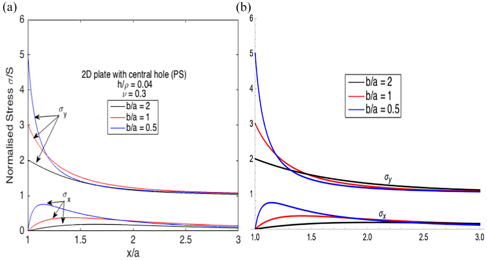
(a) Stress distribution of Figure 23 from the work by Klungerbo [9] (reproduced with the kind permission of the author) versus (b) graphs plotted from our present analytical solutions of σ_y, equation (40) and σ_x, equation (48), for elliptic and circular holes.

It is observed that the agreement is generally very good. However, there is some difference in that the curve of σ _y for b/a = 2 from the FEM in the work by Klungerbo [9] does not cross the curves for the smaller aspect ratios. As discussed earlier, ideally the curves will cross so that the total areas under each curve are the same (to compensate equally for the load that was carried by the material that was “lost” at the cross-section of the hole). These curves’ crossings are evident in all our analytical results, Figures 4, 6, and 7 and Figure 9, and in some of the work by Klungerbo [9]. This is likely because FEM results are not as accurate as closed-form analytical solutions.

An independent comparison with some BFM numerical results from the literature is provided in Figures 10 and 11. Some BFM numerical analysis results from the work by Badiger and Ramakrishna [10] due to applied uniform uniaxial loading in the y-direction are presented as Figures 18 and 20 in the work by Badiger and Ramakrishna [10] and are shown here on the left-hand side of Figures 10 and 11.

Figure 10.

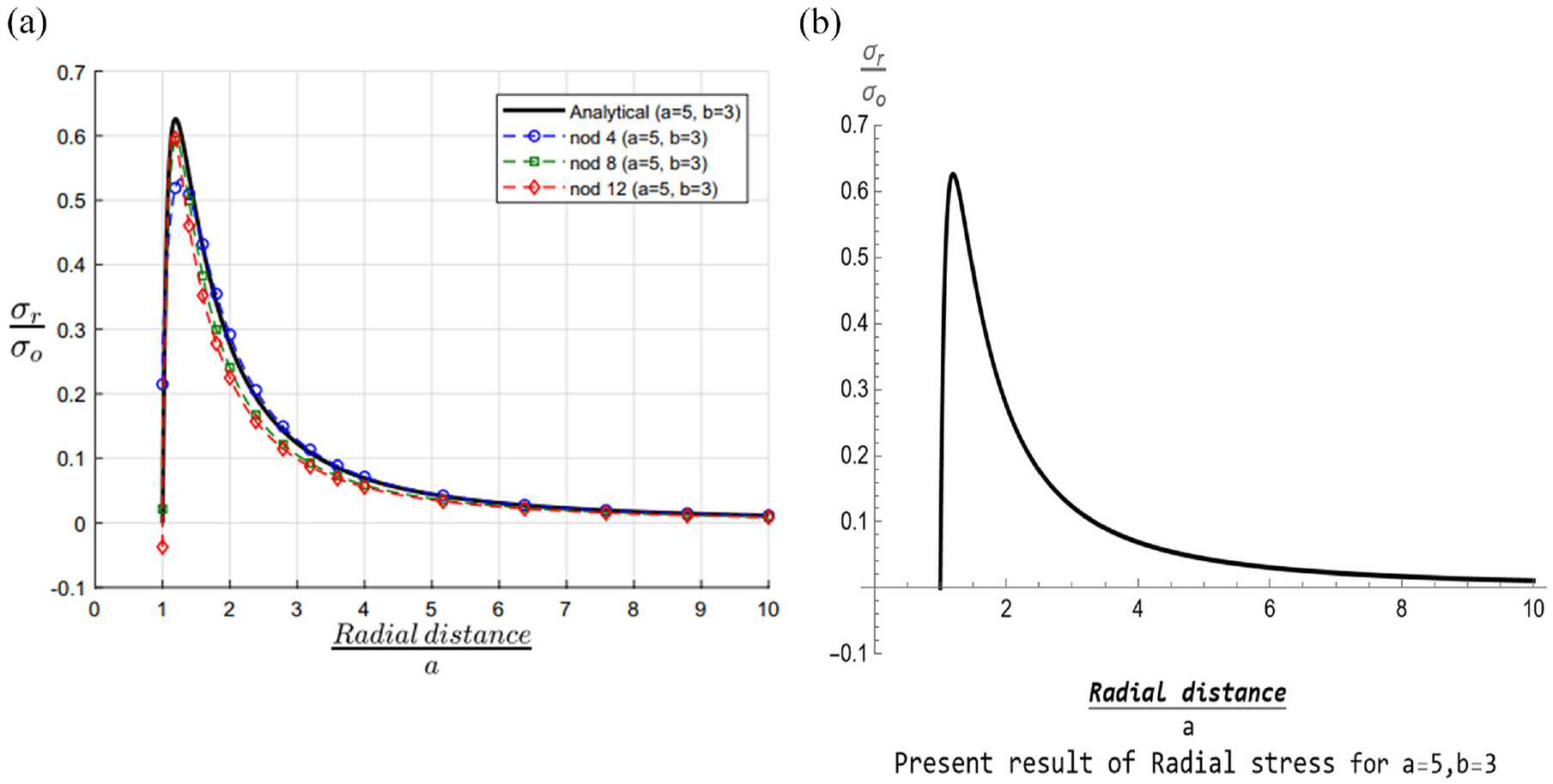
(a) Radial stress distribution of Figure 18 from the work by Badiger and Ramakrishna [10] vs (b) a graph plotted from our present analytical solution of σ _x , equation (48), for an elliptic hole of aspect ratio b/a = 3/5.

Figure 11.

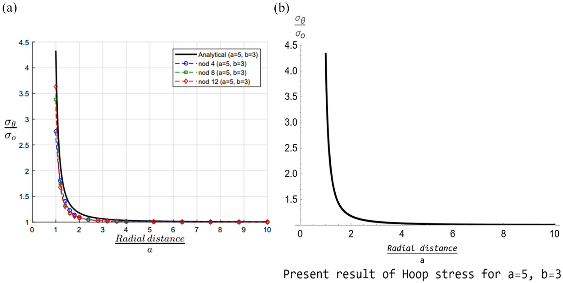
(a) Hoop stress variation of Figure 20 from the work by Badiger and Ramakrishna [10] versus (b) stress plotted from our present analytical solution of σ _y , equation (37), for an elliptic hole of aspect ratio b/a = 3/5.

It is observed in Figures 10 and 11 that Figures 18 and 20 from the work by Badiger and Ramakrishna [10] display their BFM results along with a curve they generated from their numerical calculations computed from Gao’s analytical closed-form solutions [2], presented as a solid black curve in both Figures 18 and 20 from the work by Badiger and Ramakrishna [10], as shown here on the left-hand side of Figures 10 and 11. It is noted that our present solution (black curves on the right-hand side of Figures 10 and 11) are identical to those from Gao’s [2] yet similar to the BFM of the work by Badiger and Ramakrishna [10]. Since our solutions were derived from the original Inglis’ solutions, they demonstrate that Gao’s and Inglis’ solutions provide the same results. Additional comparisons of the present solutions with some results of the work by Badiger and Ramakrishna [10] showed similar agreement as above and yet appear to be the same as Gao’s [2] results that are presented graphically in the work by Badiger and Ramakrishna [10].

2.5. Elliptical hole in a plate under remote biaxial stress uniform in all directions—stresses and displacements along the y-axis in Cartesian coordinates

The configuration and loading for this case, S _y  = S _x  = S, is depicted in Figure 1. The curvilinear coordinate systems α and β are shown in Figure 2. The tangential component σ_β of the stress field due to biaxial stress S is per equation (5). Considering the stress σ _x along y, (σ _x  =σ_{β|β = π/2}), we substitute β = π/2 in equation (5) giving:

$${\mathrm{\sigma }}_x=\frac{S\sinh 2\alpha [\cosh 2\alpha +\cosh 2{\alpha }_0+2]}{{(\cosh 2\alpha +1)}^2}.$$

(53)

For β = π/2, the transformation from elliptic curvilinear into the Cartesian coordinate system is obtained by substituting β = π/2 in equation (3) giving:

$$\alpha =\sin {\mathrm{h}}^{-1}\left(\frac{y}{c}\right)\mathrm{where}c=\sqrt{a^2-b^2}.$$

(54)

Substituting α₀ from equation (4) and α from equation (54) in equation (53) gives:

$${\mathrm{\sigma }}_x=\frac{S\sinh \left(2\sin {\mathrm{h}}^{-1}\frac{y}{c}\right)(\cosh \left(2\tan {\mathrm{h}}^{-1}\frac{b}{a}\right)+\cosh \left(2\sin {\mathrm{h}}^{-1}\frac{y}{c}\right)+2)}{{(\cosh \left(2\sin {\mathrm{h}}^{-1}\frac{y}{c}\right)+1)}^2}.$$

(55)

We apply hyperbolic function expansion to equation (55) and mathematical manipulations and simplification giving:

$${\sigma }_x=\frac{Sy(y^2-b^2+2a^2)}{{(y^2-b^2+a^2)}^{3/2}}$$

(56)

It is noted that the stress field σ _xp due to a case of internal pressure loading S, acting uniformly on the surface of the hole, can be obtained with superposition by subtracting S from the solution for the biaxial all-round remote uniform stress case. This gives σ _xp  = equation (56)−S.

The simple form of equation (56) provides the tangential stress σ _x in the material along the y-axis in terms of the remote stress S (= S _y  = S _x ), the coordinate y, and the major and minor semi axes of the ellipse a and b, respectively.

Equation (56) is equivalent to equation (9) in that it will give for y the same result as equation (9) will give for the same value of x if the values of a and b are switched. It stems from this that equation (9) can be used also for b > a.

Substituting y = b in equation (56) to find the stress at the tip of the minor axis, on the surface of the elliptical hole, gives:

$${\sigma }_{x|y=b}=\frac{2bS}{a}$$

(57)

which is the known solution for this case.

Substituting b = a in equation (56) gives:

$${\sigma }_x=S(\frac{a^2}{y^2}+1)$$

(58)

showing that equation (56) converges to the known solution of the stress field due to a circular hole in a plate subjected to remote biaxial uniform stress. To explore how equation (56) handles elliptical hole with an extreme aspect ratio, we substitute b = 0 in equation (56) which degenerates the elliptical hole into a crack of length 2a giving:

$${\sigma }_x=\frac{Sy(2a^2+y^2)}{{(a^2+y^2)}^{3/2}},$$

(59)

as the stress along the y-axis. Substituting y = 0 in equation (59) gives σ _x  = 0 which agrees with equation (57) when b = 0.

Substituting y =∞ in equation (56) and equation (59) gives σ _x  = S which agrees with the stress in the x-direction, along y, infinitely remote from the hole or from the crack.

Applying to equation (56) the procedure per equation (16) through equation (19), it can be shown that the stress field per equation (56) also satisfies the basic loading equilibrium.

The radial component σ _α of the stress field due to biaxial stress S (= S _y  = S _x ) is given by equation (20). Considering the radial stress σ _y along y, (σ _y  =σ_{α|β = π/2}) we substitute β = π/2 and equation (4) in equation (20) giving:

$${\sigma }_y=\frac{S\sinh 2\alpha [\cosh 2\alpha -\cosh \left(2\tan {\mathrm{h}}^{-1}\frac{b}{a}\right)]}{{(\cosh 2\alpha +1)}^2}.$$

(60)

We transform equation (60) from elliptic curvilinear into the Cartesian coordinate system with the transformation per equation (54) giving:

$${\sigma }_y=\frac{S\sinh \left(2\sin {\mathrm{h}}^{-1}\frac{y}{c}\right)[\cosh \left(2\sin {\mathrm{h}}^{-1}\frac{y}{c}\right)-\cosh \left(2\tan {\mathrm{h}}^{-1}\frac{b}{a}\right)]}{{[\cosh \left(2\sin {\mathrm{h}}^{-1}\frac{y}{c}\right)+1]}^2}.$$

(61)

Using hyperbolic function expansions on equation (61) and applying mathematical manipulations gives:

$${\sigma }_y=\frac{Sy(y^2-b^2)}{{(y^2-b^2+a^2)}^{3/2}}.$$

(62)

It is noted that the stress field σ _yp due to internal pressure loading S, acting uniformly on the surface of the hole, can be obtained with superposition by subtracting S from the solution for the biaxial all-round remote uniform stress case. This gives σ _yp  = equation (62)−S along the y-axis.

Substituting b = a in equation (62) gives:

$${\sigma }_y=S(1-\frac{a^2}{y^2})$$

(63)

showing that equation (62) converges to the known solution of the radial stress field due to a circular hole in a plate subjected to remote biaxial uniform stress.

Substituting y = b or y =∞ in equation (62) gives σ _y  = 0 or σ _y  = S, respectively, showing that it gives the correct value on the surface of the elliptical hole and far away from it.

To explore how equation (62) handles elliptical hole with an extreme aspect ratio, we substitute b = 0 in equation (62) which degenerates the elliptical hole into a crack of length 2a giving:

$${\sigma }_y=\frac{S{y}^3}{{(a^2+y^2)}^{3/2}}$$

(64)

which gives the correct value on the mid-surface of the crack; σ _y  = 0 at y = 0, and very far from it, σ _y  = S.

The displacements in the x-direction along the y-axis are nil due to symmetry. The displacements δ_y in the y-direction along the y-axis can be determined by transforming published solutions in curvilinear coordinates into Cartesian coordinates using the transformation per equations (4) and (7) and (54), or, calculated directly using σ _x and σ _y from equations (56) and (62), respectively. Here, we will use the latter approach first, the results of which can serve to further demonstrate the validity of equations (56) and (62). Hence, we follow the same procedure we used to calculate δ _X from equation (26) through equation (30) to calculate δ _Y at position Y on the y axis giving:

$${\delta }_Y=\frac{S[(1-\nu )(Y^2-b^2)+2a^2]}{E\sqrt{Y^2-b^2+a^2}}.$$

(65)

When Y→∞ in equation (65), then δ_Y→ (1−ν) S Y/E as expected at a point far from a hole in a plate under biaxial uniform stress.

When Y = b in equation (65), then δ _Y  = (2a S)/E which is the same as in the work by Griffith [18] on the surface of the hole due to a remote biaxial uniform stress. Note that this is applicable also to b = 0 and thus gives the proper displacement for an opening of a crack. When we substitute b = a in equation (65), we get the displacement expression due to a circular hole as:

$${\delta }_Y=\frac{S[Y^2(1-\nu )+a^2(1+\nu )]}{\mathrm{EY}}.$$

(66)

When we substitute Y = a in equation (66), then δ _Y  = (2 a S)/E which agrees with the known displacement on the edge of a circular hole for this loading.

To further validate equation (65) and the procedure used to derive it, we will derive in the following the displacements for this case using results from the work by Timoshenko [5] p.190 which can be represented as equation (32) from a previous section.

To consider displacements along y, we substitute β = π/2 and G = $\frac{\mathrm{E}}{2(1+\nu )}$ in equation (32) giving:

$$({\delta }_x+\mathbb{i}{\mathrm{\delta }}_y)=\frac{(\nu +1)}{2E}(\mathbb{i}cS\mathrm{sech}\alpha \cosh 2{\alpha }_0+\frac{\mathbb{i}c(3-\nu )\mathrm{S}\cosh \alpha }{(\nu +1)}-\mathbb{i}cS\sinh \alpha \tanh \alpha ).$$

(67)

From equation (67) we see that δ _x  = 0 as we also expect due to symmetry along y. Substituting in equation (67) that $c=\sqrt{a^2-b^2}$ and the expressions of α₀ and α from equation (4) and equation (54) gives for δ _y after mathematical manipulations the same expression as equation (65). This validates equation (65) and demonstrates the validity of the stress equations (56) and (62), that were used here to derive equation (65).

2.6. Elliptical hole in a plate under remote uniaxial uniform stress S _y —stresses and displacements along they-axis in Cartesian coordinates

The configuration and loading for the case of S _y  = S, are depicted in Figure 5. We derived the tangential stress field for this case from the work by Inglis [1] and obtained the tangential component σ_β of the stress field in equation (34). Considering the stress σ _x along y, (σ _x  =σ_{β|β = π/2}), we substitute β = π/2 in equation (34) giving:

$$\begin{array}{c}\multicolumn{1}{c}{{\sigma }_x=\frac{S}{{(\cosh 2\alpha +1)}^2}((-\frac{{\mathbb{e}}^{2{\alpha }_0}}{8}-\frac{1}{16})(2{\mathbb{e}}^{-4\alpha }+8{\mathbb{e}}^{-2\alpha }+6)+\frac{1}{8}{\mathbb{e}}^{4{\alpha }_0}(-{\mathbb{e}}^{-4\alpha }-4{\mathbb{e}}^{-2\alpha }-3)}\\ \multicolumn{1}{c}{+\frac{1}{8}(-4{\mathbb{e}}^{2\alpha }-{\mathbb{e}}^{4\alpha }-3)+\frac{1}{16}(8{\mathbb{e}}^{2\alpha }+2{\mathrm{e}}^{4\alpha }+6)+\frac{1}{4}({\mathbb{e}}^{2\alpha }-{\mathbb{e}}^{-2\alpha })(\cosh 2{\alpha }_0+1)).}\end{array}$$

(68)

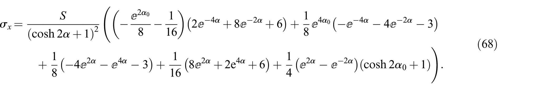
Substituting α₀ from equation (4) and α from equation (54) in equation (68) transforms it into:

$$\begin{array}{c}\multicolumn{1}{c}{{\sigma }_x=\frac{S}{{(\cosh \left(2\sin {\mathrm{h}}^{-1}\left(\frac{y}{c}\right)\right)+1)}^2}(\frac{1}{8}{\mathbb{e}}^{4\tan {\mathrm{h}}^{-1}\left(\frac{b}{a}\right)}(-{\mathbb{e}}^{-4\sin {\mathrm{h}}^{-1}\left(\frac{y}{c}\right)}-4{\mathbb{e}}^{-2\sin {\mathrm{h}}^{-1}\left(\frac{y}{c}\right)}-3)}\\ \multicolumn{1}{c}{+(-\frac{1}{8}{\mathbb{e}}^{2\tan {\mathrm{h}}^{-1}\left(\frac{b}{a}\right)}-\frac{1}{16})(2{\mathrm{e}}^{-4\sin {\mathrm{h}}^{-1}\left(\frac{y}{c}\right)}+8{\mathbb{e}}^{-2\sin {\mathrm{h}}^{-1}\left(\frac{y}{c}\right)}+6)+\frac{1}{4}({\mathbb{e}}^{2\sin {\mathrm{h}}^{-1}\left(\frac{y}{c}\right)}-{\mathbb{e}}^{-2\sin {\mathrm{h}}^{-1}\left(\frac{y}{c}\right)})}\\ \multicolumn{1}{c}{(\cosh \left(2\tan {\mathrm{h}}^{-1}\left(\frac{b}{a}\right)\right)+1)+\frac{1}{8}(-4{\mathbb{e}}^{2\sin {\mathrm{h}}^{-1}\left(\frac{y}{c}\right)}-{\mathbb{e}}^{4\sin {\mathrm{h}}^{-1}\left(\frac{y}{c}\right)}-3)+\frac{1}{16}(8{\mathbb{e}}^{2\sin {\mathrm{h}}^{-1}\left(\frac{y}{c}\right)}+2{\mathbb{e}}^{4\sin {\mathrm{h}}^{-1}\left(\frac{y}{c}\right)}+6)).}\end{array}$$

(69)

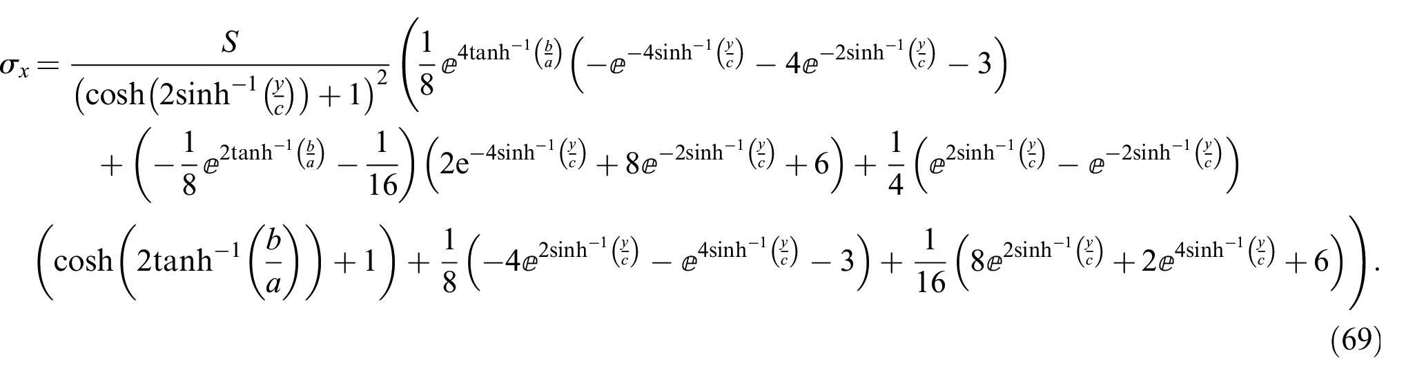
Using lengthy mathematical manipulations, we obtain from equation (69) the tangential stress σ _x along the y-axis, due to uniaxial load S (= S _y ) in the y-direction as:

$${\sigma }_x=\frac{S{a}^2}{{(a-b)}^2}(\frac{y(2a^2-\mathrm{ab}-b^2+y^2)}{{(a^2-b^2+y^2)}^{3/2}}-1).$$

(70)

Note the similarity in the form of equations (70) and (44).

To determine the radial stress σ _y along the y-axis (σ _y  =σ_{α|β = π/2}) due to remote uniaxial stress in the y-direction, S _y  = S, we use the work by Gao [2] to calculate σ _x  + σ _y along the y-axis due to uniform uniaxial stress in the y-direction using equations (29) and (30) from the work by Gao [2] giving:

$${\sigma }_x+{\sigma }_y=\frac{1}{2}S(1+{\mathbb{e}}^{2{\alpha }_0})(\mathrm{Sech}\alpha {)}^2\mathrm{Sinh}2\alpha -{\mathbb{e}}^{2{\alpha }_0}S.$$

(71)

Substituting equations (4) and (54) in equation (71) and using mathematical manipulations gives:

$${\sigma }_x+{\sigma }_y=\frac{2Say}{(a-b)\sqrt{y^2-b^2+a^2}}-\frac{S(a+b)}{a-b}.$$

(72)

We write σ _y  = (σ _x  + σ _y )−σ _x  = equation (72)−equation (70) which gives after mathematical manipulations:

$${\sigma }_y=\frac{b^{2}S}{{(a-b)}^2}-\frac{Sy(b{a}^3+a^2{b}^2-2a{b}^3)+S{y}^3(2ba-a^2)}{{(a-b)}^2{(a^2-b^2+y^2)}^{3/2}}.$$

(73)

Equation (73) provides the distribution of the radial stress field σ _y along the y-axis due to a remote uniaxial stress S _y  = S in the y-direction. Substituting y = b or y = ∞ gives 0 or S, respectively, as expected on the surface of the hole or far away from it, for this uniaxial loading. For b→a, equation (73) gives the same results as the known solution for a circular hole for this loading.

The tangential stress σ _x along y (σ _x  =σ_{β|β = π/2}), due to uniaxial remote stress in the x-direction, S _x  = S, is obtained by superposition as σ _x  =σ _x [biaxial]−σ _x [uniaxial in y]= equation (56)−equation (70) giving:

$${\sigma }_x=\frac{a^{2}S}{{(a-b)}^2}+\frac{Sy(2a^2{b}^2-3a^{3}b+2a{b}^3-b^4)+S{y}^3(b^2-2ab)}{{(a-b)}^2{(a^2-b^2+y^2)}^{3/2}}.$$

(74)

Substituting y = b in equation (74) gives S ( $\frac{2b}{a}$ + 1) which is the well-known solution at the tip of the minor axis for uniaxial loading in the x-direction, S _x  = S.

2.7. Example

The case solved by equation (74) may represent an elliptic opening configuration in an aircraft wing panel. The x-axis of the hole, being in the wingspan direction, coincides with the direction of the main tension in the wing panel and reduces the stress concentration by having the minor axis of the ellipse perpendicular to the load. Yet, the higher tension stresses (σ _x ) will be along the y-axis (wing cord direction) and their values along the y-axis, per equation (74), could be used for fatigue and cracking analysis [end of example].

The radial stress σ _y along y, (σ _y  =σ_{α|β = π/2}), due to uniaxial stress in the x-direction, S _x  = S, is obtained by superposition as σ _y  =σ _y [biaxial]−σ _y [uniaxial S _y  = S] = equation (62)−equation (73) giving:

$${\sigma }_y=\frac{Syb(a^3-b^3+b{y}^2)}{{(a-b)}^2{(a^2-b^2+y^2)}^{3/2}}-\frac{b^{2}S}{{(a-b)}^2}.$$

(75)

Substituting y = b or y =∞ in equation (75) gives 0 as expected on the surface of the hole or far away from it on the y-axis, for this uniaxial loading in the x-direction, S _x  = S.

The displacements along the y-axis due to the uniaxial load in the y-direction, S _y  = S, are calculated directly using σ _x and σ _y from equations (70) and (73), respectively. The results may serve to further demonstrate the validity of equations (70) and (73). We follow the procedure we used previously in equation (26) through equation (29), but with σ _x and σ _y now taken from equations (70) and (73), respectively, and applied in the y-direction to calculate δ _Y at position Y on the y-axis as follows.

The displacement δ _Y of a specific point at position Y on the y-axis can be shown to be given by:

$${\delta }_Y={\delta }_R-{\delta }_{\mathrm{YR}},$$

(76)

where δ _R is the displacement of a remote point at position R on the y-axis and δ _YR is the elongation of the material between Y and R. We note that the strain ε _y in the y-direction is given by:

$${\epsilon }_y=\frac{{\sigma }_y-\nu {\sigma }_x}{E},$$

(77)

and,

$${\delta }_{\mathrm{YR}}={\int }_Y^R{\epsilon }_y\mathbb{d}y.$$

(78)

For a very remote point where R→∞, the local effect of the hole diminishes and δ _R is given by:

$${\delta }_{R\to \infty }=\frac{S}{E}R.$$

(79)

Following the above procedure, we obtain:

$${\delta }_Y=\underset{R\to \infty }{\mathrm{limit}}({\delta }_R-{\delta }_{\mathrm{YR}})=\frac{SY(a^2\nu +b^2)}{E{(a-b)}^2}+\frac{a^{3}S[2a-b(\nu +3)]-S(Y^2-b^2)[2\mathrm{ab}-a^2(1-\nu )]}{E{(a-b)}^2\sqrt{a^2-b^2+Y^2}}$$

(80)

For Y →∞, equation (80) converges to (S Y)/E which is what we expect at a point on the y-axis infinitely remote from the hole. Substituting Y = b in equation (80) gives S (2 a + b)/E at the tip of the minor axis. When b = 0, this becomes (2 S a)/E which is identical to the opening of a crack of length 2a under such loading. Hence, equation (80) gives the proper displacement when the elliptical hole degenerates to a crack. When Y = b and b =a, the displacement becomes (3 S a)/E which is the proper displacement for a circular hole.

The displacements along the y-axis due to the uniaxial load in the x-direction, S _x  = S, are calculated directly using σ _x and σ _y from equations (74) and (75), respectively. The results may serve to further demonstrate the validity of equations (74) and (75). We follow the procedure used above in equation (76) through equation (80), but with σ _x and σ _y now taken from equation (74) and equation (75), respectively, and equation (79) is replaced with δ _R $\to \infty$  = -νS R/E to account for the load in the x direction only. This gave:

$${\delta }_Y=\frac{S(Y^2-b^2)[b^2(1-\nu )+2ba\nu ]+S[2a^2{b}^2-b{a}^3(1-\nu )]}{E{(a-b)}^2\sqrt{Y^2-b^2+a^2}}-\frac{SY(b^2+a^2\nu )}{E{(a-b)}^2}$$

(81)

for the displacement along the y-axis due to stress S _x  = S in the x-direction. For Y→∞, equation (81) converges to (−νS Y)/E which is what we expect at a point on the y-axis infinitely remote from the hole for this loading. Substituting Y = b in equation (81) gives (−S b)/E at the tip of the minor axis. If we superimpose this on equation (80) of the hole displacement, at the minor axis tip due to load in the y-direction,(i.e. S (2 a + b)/E), we obtain (2 S a)/E which is the known displacement at the hole minor axis edge due to biaxial uniform stress. The sum of equations (80) and (81) gives the same expression as the δ _Y for uniform biaxial stress per equations (65) and (67). Hence, the superposition of displacements due to loading in the x- and y-directions appears to give the proper answer at all points along the y-axis and is not restricted to the edge of the hole.

2.8. Remote Uniaxial load at angle θ to the y-axis of the ellipse

The configuration and loading for this case are depicted in Figure 12. The remote uniaxial stress S is acting at an angle θ to the principal axis y as shown.

Figure 12.

Remote uniaxial stress S acting at an angle θ to the principal axis y.

The solution for the tangential stress σ_β, in elliptical curvilinear coordinates, for this case, is extracted from the work by Gao [2] as:

$$\begin{array}{c}\multicolumn{1}{c}{\frac{{\sigma }_{\beta }}{S}==\frac{{\mathbb{e}}^{2{\alpha }_0}(\cosh (2\alpha -2{\alpha }_0)\cos (2\beta -2\theta )+\cos 2\theta (\sinh 2\alpha -\cosh 2{\alpha }_0+\sin 2\beta \sin 2\theta )}{2(\cosh 2\alpha -\cos 2\beta )}}\\ \multicolumn{1}{c}{-\frac{{\mathbb{e}}^{2{\alpha }_0}((\cosh 2\alpha -\cosh 2{\alpha }_0)\sin 2\beta \sin 2\theta +\sinh 2\alpha \cos 2\theta (\cos 2\beta -\cosh 2{\alpha }_0))}{2{(\cosh 2\alpha -\cos 2\beta )}^2}}\\ \multicolumn{1}{c}{+\frac{\sinh 2\alpha (\cosh 2\alpha +\cosh 2{\alpha }_0-2\cos 2\beta )}{2{(\cosh 2\alpha -\cos 2\beta )}^2}-\frac{1}{2}{\mathbb{e}}^{2{\alpha }_0}\cos 2\theta .}\end{array}$$

(82)

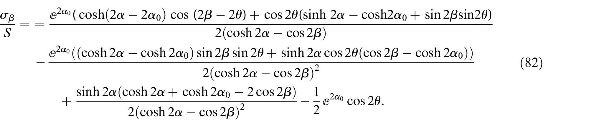
It is noted that when applying superposition for stress loading S at angle θ plus stress γS at angle θ =θ + π/2, the result we get from equation (82) for σ_{β|θ = θ} + γσ_{β|θ =θ + π/2} is identical to the general solution result for the full-field case (equation (31) in the work by Gao [2]). Hence, the work by Gao [2] serves to show that superposition is applicable for the elliptic hole configuration.

Considering the stress σ _y along x (σ _y  =σ_{β|β = 0}), we substitute β = 0 in equation (82) and transform it into Cartesian coordinates with equations (4) and (7) giving:

$$\begin{array}{l}\frac{{\sigma }_y}{S}==-\frac{\cos \left(2\theta \right){\mathbb{e}}^{2{\tanh }^{-1}\left(\frac{b}{a}\right)}\left(1-\cosh \left(2{\tanh }^{-1}\left(\frac{b}{a}\right)\right)\right)\sinh (2{\cosh }^{-1}\left(\frac{x}{c}\right))}{2{\left(\cosh \left(2{\cosh }^{-1}\left(\frac{x}{c}\right)\right)-1\right)}^2}\\ +\frac{1}{2\left(\cosh \left(2{\cosh }^{-1}\left(\frac{x}{c}\right)\right)-1\right)}{\mathbb{e}}^{2{\tanh }^{-1}\left(\frac{b}{a}\right)}\\ (\cos \left(2\theta \right)\cosh \left(2{\cosh }^{-1}\left(\frac{x}{c}\right)-2{\tanh }^{-1}\left(\frac{b}{a}\right)\right)+\cos \left(2\theta \right)(\sinh \left(2{\cosh }^{-1}\left(\frac{x}{c}\right)\right)-\cosh (2{\tanh }^{-1}\left(\frac{b}{a}\right))))\\ -\frac{1}{2}\cos \left(2\theta \right){\mathbb{e}}^{2{\tanh }^{-1}\left(\frac{b}{a}\right)}+\frac{\sinh \left(2{\cosh }^{-1}\left(\frac{x}{c}\right)\right)\left(\cosh \right(2tan{\mathrm{h}}^{-1}\left(\frac{b}{a}\right))+\cosh \left(2{\cosh }^{-1}\left(\frac{x}{c}\right)\right)-2)}{2{\left(\cosh \left(2{\cosh }^{-1}\left(\frac{x}{c}\right)\right)-1\right)}^2}.\end{array}$$

(83)

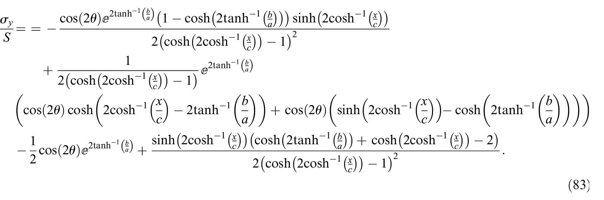
Using very extensive mathematical manipulations and simplifications, we reduce equation (83) to obtain:

$$\frac{{\sigma }_y}{S}=\frac{x(x^2-a^2+2b^2)}{2{(x^2-a^2+b^2)}^{3/2}}-(\frac{(c^{2}x-x^3)(c^2-2ab)-b^2{c}^{2}x}{2b^2{(x^2-a^2+b^2)}^{3/2}}-1)\frac{b^2\cos \left(2\theta \right)}{{(a-b)}^2}$$

(84)

Equation (84) provides the stress σ _y along the x-axis, due to a remote uniaxial stress S in a direction making an angle θ with the y-axis per Figure 12. Note that the first term in equation (84) is half the σ _y result for the biaxial uniform remote stress per equation (9). When substituting θ = 0 in equation (84), it corresponds to the case of uniaxial load in the y-direction, S _y  = S, and it gives indeed the same result as equation (37) which we derived from the work by Inglis [1] for this case. When substituting θ = π/2 in equation (84), it corresponds to the case of uniaxial load in the x direction, S _x  = S, and it gives indeed the same result as equation (44) which we derived from the work by Inglis [1] for this case. When we superimpose these two cases of θ = 0 and θ = π/2 from equation (84), their sum gives indeed the same result as equation (9) which we derived from the work by Inglis [1] for this uniform biaxial loading. Hence, the earliest results from the work by Inglis [1] are consistent with the general solution in the work by Gao [2] (all in curvilinear coordinates). When we superimpose equation (84)_θ + equation (84)_{θ + π/2} for any direction θ, it gives the same result as equation (9) for uniform biaxial stress S in the x- and y-directions; S _y  = S _x  = S. Hence, it corresponds indeed to all-round uniform stress. As superposition can be applied for stress loadings in the same direction and for stress loadings acting in perpendicular directions, we can use equation (84) in superposition of S_θ = S and S_{θ + π/2} =γS similar to equation (1).

2.9. Consideration of shear

The stress σ _y along the x-axis due to pure shear loading can be obtained from equation (84) by superposition of equation (84)_{θ = π/4} + (−S/S) equation (84)_{θ = −π/4}. This gives σ _y  = 0 along the x-axis, including at x = a on the surface of the hole.

The maximum shear stress in the x–y plane along x is calculated as:

$${\tau }_{\max }=\frac{1}{2}({\sigma }_y-{\sigma }_x).$$

(85)

The maximum shear in the x–y plane along x due to uniform biaxial loading, S _y  = S _x  = S, is obtained by substituting σ _x and σ _y from equations (23) and (28) in equation (85) which gives after mathematical manipulations:

$${\tau }_{\max }=\frac{b^{2}Sx}{{(x^2-a^2+b^2)}^{3/2}}.$$

(86)

The maximum shear in the x–y plane along x due to uniform uniaxial loading in the y-direction, S _y  = S, is obtained by substituting σ _x and σ _y from equations (48) and (37) in equation (85) giving after mathematical manipulations:

$${\tau }_{\max }=\frac{Sa\mathrm{bx}(a^2+ab-2b^2-x^2)}{{(a-b)}^2{(x^2-a^2+b^2)}^{3/2}}+\frac{S(a^2+b^2)}{2{(a-b)}^2}.$$

(87)

The maximum shear the in the x–y plane along x due to uniform uniaxial loading in the x-direction, S _x  = S, is obtained by substituting σ _x and σ _y from equations (51) and (44) in equation (85) giving after mathematical manipulations:

$${\tau }_{\max }=\frac{Sbx(a{x}^2-a^3+b^3)}{{(a-b)}^2{(x^2-a^2+b^2)}^{3/2}}-\frac{S(a^2+b^2)}{2{(a-b)}^2}.$$

(88)

Similar analysis can be performed to calculate the maximum shear stress along the y-axis using the σ _y and σ _x values obtained here in the previous sections for such cases.

For plane stress condition, when considering the maximum shear in the x–z or y–z planes, the maximum shear stress τ_max is σ _x /2 or σ _y /2. The largest value of the three τ_max, for each loading case, can be regarded as the τ_{max max} for that loading.

2.10. Some comments

It is noted that for all the loadings considered herein, that are symmetrical with respect to the principal axes x and y of the elliptic hole, all stresses and displacements will be symmetrical as well. Hence, in these cases, the stresses and displacements along the negative (and positive) sides of the x and y axes can be calculated using the corresponding equations derived herein (for the positive sides of the axes) by simply replacing the negative x values with |x| (or $\sqrt{x^2}$ ) and the negative y values with |y| (or $\sqrt{y^2}$ ) in all the equations for stresses and displacements. It is also noted that based on the comparison of the present results along the x and y axes, it is concluded that the present stress fields and displacements expressions along the x-axis are applicable also for elliptic holes with a < b.

It is interesting to note the relationship that prevails between stresses and displacements on the surface of the elliptical hole, as observed from the results for all the symmetrical loading cases considered here (plain stress conditions). These are summarized in the following:

$$\frac{\mathrm{\Delta }\mathrm{b}}{b}=\frac{{\sigma }_{y|x=a;y=0}}{E}={\epsilon }_{y|x=a;y=0}\&\frac{\mathrm{\Delta }\mathrm{a}}{a}=\frac{{\sigma }_{x|x=0;y=b}}{E}={\epsilon }_{x|x=0;y=b},$$

(89)

where σ _y and σ _x are the tangential stresses at the tips of the major and minor axes of the hole, respectively, and Δa and Δb are the displacements at these points, respectively. Since the deformed hole maintains an elliptical shape, we can write for any point (x; y) on the surface of the hole that:

$$\frac{\mathrm{\Delta }\mathrm{y}}{y}=\frac{{\sigma }_{y|x=a;y=0}}{E}={\epsilon }_{y|x=a;y=0}\&\frac{\mathrm{\Delta }\mathrm{x}}{x}=\frac{{\sigma }_{x|x=0;y=b}}{E}={\epsilon }_{x|x=0;y=b},$$

(90)

for any symmetrical loading combinations acting in the ellipse principal directions x or y, and where Δx and Δy are the x and y displacements at the point (x;y). Hence, the Δx or Δy displacements of the elliptic hole, per equation (90), are the same as of an identical ellipse, drawn in lieu of the same hole, on an intact plate loaded with uniaxial uniform stress equal to σ_{x|x = 0; y = b} or σ_{y|x = a; y = 0} in the x- or y-direction, respectively. As observed from equation (90), on the surface of the elliptic hole, the displacements are independent of ν, for any loading combination in the principal directions of the ellipse. Note that it was first pointed out in the work by Gao [2] that an elliptic hole is stretched without distortion under all-round tension.

3. Conclusion

Based on the works by Inglis and Gao [1,2], explicit expressions are derived for stress fields and displacements in terms of a Cartesian coordinate system, along the x and y axes, due to an elliptic hole in an infinite elastic plate subjected to remote uniaxial or biaxial loadings in the directions of the principal axes of the ellipse. Also, for remote uniaxial stress S acting at an angle θ to the principal axis y, the stress field σ _y along the x-axis is provided in a Cartesian coordinate system. These closed-form results are presented in relatively simple and concise expressions. They are the functions of cubic or parabolic polynomials of x or y along the x or y axes, respectively. These results are used to calculate stresses and displacement for special cases, such as a circular hole, a crack, an elliptical hole in a pressurized cylindrical shell, and are shown to agree with published solutions where available. The present results also demonstrate that the original solution by Inglis [1] and later studies such as the general solution by Gao [2], and the results of Kanezaki et al. [17] are consistent with one another.

For the benefit and convenience of potential users, we provide in the following a list of the cases analyzed herein, along with the corresponding equation numbers for the main results in Cartesian coordinates.

• Equation (9): Normal stress σ _y ahead of the hole along the x-axis due to uniform all-round biaxial load

• Equation (16): Normalized equation (9), σ _n is the normalized stress σ _y ahead of the hole along the x axis due to uniform all-round biaxial loading

• Equation (23): Radial stress σ _x ahead of the hole along the x-axis due to uniform all-round biaxial load

• Equation (30): δ _X displacements along the x-axis due to uniform all-round biaxial loading

• Equation (37): σ _y , the stress along the x-axis due to uniaxial load in the y-direction

• Equation (40): Normalized equation (37); σ _yn is normalized σ _y , the normal stress along the x-axis due to uniaxial load in the y direction

• Equation (44): σ _yn is normalized σ _y , the normal stress along the x-axis due to uniaxial load in the x-direction

• Equation (45): σ _yn is normalized σ _y , the normal stress along the x-axis due to load S in the y-direction + load 2 S in the x-direction as in pressurized thin cylindrical shell.

• Equation (47): σ _x  + σ _y along the x-axis due to uniaxial loading in the y-direction derived from the work by Gao [2]

• Equation (48): provides the distribution of the radial stress field σ _x along the x-axis due to remote uniaxial stress in the y-direction.

• Equation (50): δ _X displacements along the x-axis due to uniaxial loading in the y-direction

• Equation (51): provides the distribution of the radial stress field σ _x along the x-axis due to remote uniaxial stress in the x-direction.

• Equation (52): δ _X displacements along the x-axis due to uniaxial loading in the x-direction

• Equation (56): provides the stress σ _x in the material along the y-axis due to uniform all-round biaxial load

• Equation (62): provides the radial stress σ _y in the material along the y-axis due to uniform all-round biaxial load

• Equation (65): δ _Y displacements along the y-axis due to uniform all-round biaxial load

• Equation (70): σ _x is the tangential stress along the y-axis due to uniaxial loading in the y-direction

• Equation (72): σ _x  + σ _y along the y-axis due to uniaxial loading in the y-direction derived from the work by Gao [2]

• Equation (73): provides the distribution of the radial stress field σ _y along the y-axis due to remote uniaxial stress in the y-direction

• Equation (74): tangential stress σ _x along y due to uniaxial stress S in the x-direction obtained by superposition

• Equation (75): the radial stress σ _y along y due to uniaxial stress S in the x-direction is obtained by superposition

• Equation (80): δ _Y displacements along the y-axis due to the uniaxial load S in the y-direction, calculated directly using σ _x and σ _y

• Equation (81): δ _Y displacements along the y-axis due to the uniaxial load S in the x-direction, calculated directly using σ _x and σ _y

• Equation (84): stress σ _y along the x-axis, due to a remote uniaxial stress S in a direction making an angle θ with the y-axis

• Equation (86): maximum shear in the x–y plane along x due to uniform biaxial loading

• Equation (87): maximum shear in the x–y plane along x due to uniform uniaxial loading in the y-direction

• Equation (88): maximum shear the in x–y plane along x due to uniform uniaxial loading in the x-direction