A note on the Hill–Ogden generalised strains

Abstract

This brief contribution provides an overview of the Hill–Ogden generalised strain tensors, and some considerations on their representation in generalised (curvilinear) coordinates, in a fully covariant formalism that is adaptable to a more general theory on Riemannian manifolds. These strains may be naturally defined with covariant components or naturally defined with contravariant components. Each of these two macro-families is best suited to a specific geometrical context.

1. Introduction

In large-deformation Continuum Mechanics, the fundamental measure of deformation is the deformation gradient $\mathit{F}$ , a two-point tensor, mapping material vectors in the body into spatial vectors in the physical space. The polar decomposition $\mathit{F}=\mathit{R}\mathit{U}=\mathit{V}\mathit{R}$ decomposes the deformation gradient $\mathit{F}$ into a pure deformation, described by the material right stretch tensor $\mathit{U}$ , followed by a rotation, described by the two-point rotation tensor $\mathit{R}$ , or into a rotation, described by the same two-point rotation tensor $\mathit{R}$ , followed by a pure deformation, described by the spatial left stretch tensor $\mathit{V}$ . The material Green–Lagrange strain $\mathit{E}=\frac{1}{2}({\mathit{U}}^2-\mathit{I})$ and the spatial Almansi–Euler strain $\mathit{e}=\frac{1}{2}(\mathit{i}-{\mathit{V}}^{-2})$ could be called the fundamental strain tensors (here, we used their “mixed” form, whose components have the first index contravariant and the second covariant; $\mathit{I}$ and $\mathit{i}$ are the material and spatial identity tensors, respectively).

According to Truesdell [1], the Green–Lagrange strain $\mathit{E}$ was first introduced by Cauchy [2] and de Saint Venant [3], and the Almansi–Euler strain $\mathit{e}$ was first introduced by Almansi [4] and Hamel [5]. Another early measure of strain was the logarithmic strain, which Hencky [6] introduced in scalar form, and which Truesdell [1] defined as the strain tensor $\ln (\mathit{U})$ (in this form, this strain is a “mixed” tensor) and named the Hencky strain. Yet another measure of strain, $\mathit{U}-\mathit{I}$ (in this form, this strain is a “mixed” tensor), was introduced by Biot [7], and then called the Biot strain later by Truesdell [1]. However, Truesdell [1] did not explicitly relate the Hencky strain $\ln (\mathit{U})$ and the Biot strain $\mathit{U}-\mathit{I}$ to the standard Green–Lagrange strain $\mathit{E}$ and Almansi–Euler strain $\mathit{e}$ . Doyle and Ericksen [8] briefly mentioned that there is an infinity of material strain measures that can be expressed by (in their “mixed” form, and in our notation)

$${\mathit{E}}^{(m)}=\frac{1}{m}({\mathit{U}}^m-\mathit{I}),$$

(1)

where $m$ is any non-zero real number. This family of strains includes the Green–Lagrange strain (for $m=2$ ), the Biot strain (for $m=1$ ), and the Hencky strain (for $m\to 0$ ). Hill [9] reported the strain measures (1) and noted that these can be written in the spectral decomposition

$${\mathit{E}}^{(m)}=\sum _{\alpha =1}^3\frac{1}{m}({\lambda }_{\alpha }^m-1){\mathit{N}}_{\alpha }\otimes {\mathit{N}}^{\alpha },$$

(2)

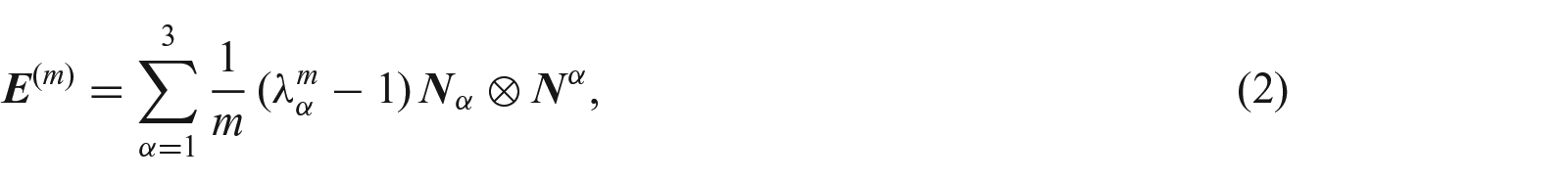
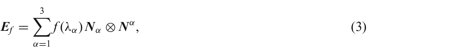
where the ${\lambda }_{\alpha }$ are the principal stretches, the eigenvalues of $\mathit{U}$ , and ${\mathit{N}}_{\alpha }$ are the principal directions of stretch, the corresponding eigenvectors. Based on equations (1) and (2), Hill [9] proposed the generalised strain

$${\mathit{E}}_f=\sum _{\alpha =1}^{3}f({\lambda }_{\alpha }){\mathit{N}}_{\alpha }\otimes {\mathit{N}}^{\alpha },$$

(3)

where $f:{\mathbb{R}}^{+}\to \mathbb{R}:\lambda \mapsto f(\lambda )$ is a monotonically increasing function such that

$$f(1)=0,f^{\prime }(1)=1.$$

(4)

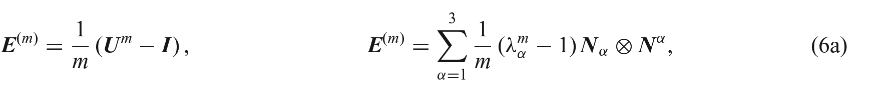
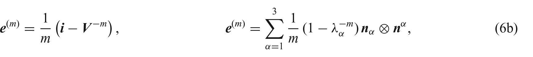
The properties (4) ensure that any Hill strain (3) reduces to the infinitesimal strain in the limit of small deformations [10]. This family of strain tensors, which are all material, was later extended by Ogden [10] to also include spatial strain tensors, such as the standard Almansi–Euler strain $\mathit{e}$ . Ogden [10] observed that, since both functions

$$\lambda \mapsto \frac{1}{m}({\lambda }^m-1),\lambda \mapsto \frac{1}{m}(1-{\lambda }^{-m}),$$

(5)

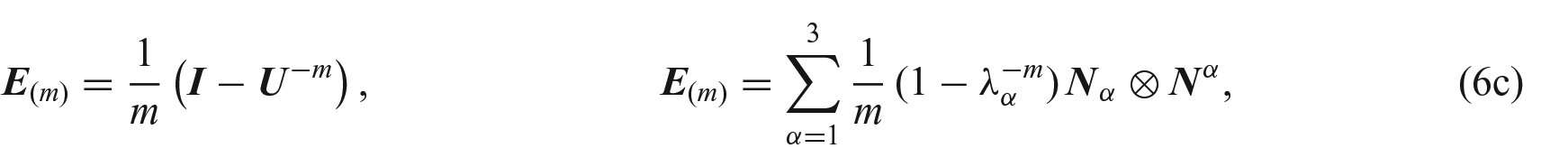
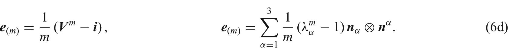
satisfy the properties (4), any strain tensor based on either $\mathit{U}$ or $\mathit{V}$ and on either of the forms (5) of the function $f$ , and constructed with a spectral decomposition of the type (3), is a legitimate strain tensor. The four strain families envisioned by Ogden [10] are (in their “mixed” form and in our notation; ${\mathit{n}}_{\alpha }=\mathit{R}{\mathit{N}}_{\alpha }$ are the spatial principal directions of stretch)

$${\mathit{E}}^{(m)}=\frac{1}{m}({\mathit{U}}^m-\mathit{I}),{\mathit{E}}^{(m)}=\sum _{\alpha =1}^3\frac{1}{m}({\lambda }_{\alpha }^m-1){\mathit{N}}_{\alpha }\otimes {\mathit{N}}^{\alpha },$$

(6a)

$${\mathit{e}}^{(m)}=\frac{1}{m}(\mathit{i}-{\mathit{V}}^{-m}),{\mathit{e}}^{(m)}=\sum _{\alpha =1}^3\frac{1}{m}(1-{\lambda }_{\alpha }^{-m}){\mathit{n}}_{\alpha }\otimes {\mathit{n}}^{\alpha },$$

(6b)

$${\mathit{E}}_{(m)}=\frac{1}{m}(\mathit{I}-{\mathit{U}}^{-m}),{\mathit{E}}_{(m)}=\sum _{\alpha =1}^3\frac{1}{m}(1-{\lambda }_{\alpha }^{-m}){\mathit{N}}_{\alpha }\otimes {\mathit{N}}^{\alpha },$$

(6c)

$${\mathit{e}}_{(m)}=\frac{1}{m}({\mathit{V}}^m-\mathit{i}),{\mathit{e}}_{(m)}=\sum _{\alpha =1}^3\frac{1}{m}({\lambda }_{\alpha }^m-1){\mathit{n}}_{\alpha }\otimes {\mathit{n}}^{\alpha }.$$

(6d)

In section 2.2.7 of his treatise, Ogden [10] recalls the standard material Green–Lagrange and spatial Almansi–Euler strain tensors, obtained from equation (6a) for $m=2$ and from equation (6b) for $m=-2$ , respectively, in equation (2.2.82) indicates, as examples, the families (6a) and (6d) and, in equation (2.2.88), he defines the material Almansi strain, obtained from equation (6c) for $m=-2$ .

This work aims at discussing the broader family (6) of Hill–Ogden generalised strains in a fully covariant formalism. We shall work in affine spaces for the sake of simplicity, but the conclusions remain valid in Riemannian manifolds. We shall see how all strain tensors in the families (6a) and (6b) are naturally defined with covariant components, and thus act ordinarily on tangent vectors, while all strain tensors in the families (6c) and (6d) are naturally defined with contravariant components, and thus act on tangent covectors parallel to the normal covectors to area elements. The latter result was already hinted in a work by Merodio and Ogden [11].

2. Theoretical background

The notation in this work follows essentially Truesdell and Noll [12] and Marsden and Hughes [13], as well as some past works [14–16]. In the modern picture of Continuum Mechanics [12,13,17–19], the physical space and deformable bodies are represented as differentiable manifolds. However, for our purposes, it suffices to consider physical space as an affine space (which is a trivial differentiable manifold; see [18]) and a body as an open subset of an affine space (again a trivial differentiable manifold).

For the full definition and properties of affine spaces, see the treatise by Epstein [18]. Briefly, an affine space is a set $\mathcal{A}$ , called point space, considered together with a vector space $\mathcal{V}$ , called modelling (or supporting) vector space and a mapping $\mathcal{F}:\mathcal{A}\times \mathcal{A}\mapsto \mathcal{V}:(x,p)\mapsto v\equiv p-x$ , called a framing and defining, for every two points $x$ and $p$ in $\mathcal{A}$ , the vector $v\equiv p-x$ in $\mathcal{V}$ , attached at $x$ . The difference-of-points notation can be exploited to obtain a point as the sum of a point and a vector, i.e., $v\equiv p-x$ implies $p=x+v$ .

2.1. Physical space and bodies

We represent physical space as the three-dimensional affine space $\mathcal{S}\equiv {\mathbb{E}}^3$ , i.e., the familiar ${\mathbb{R}}^3$ considered as both the point space and the modelling vector space. The points in $\mathcal{S}$ are denoted $x$ . The space of all vectors attached at $x$ is the tangent space $T_x\mathcal{S}$ and the disjoint union of all tangent spaces is the tangent bundle $T\mathcal{S}$ . A coordinate chart $\{x^a\}$ in $\mathcal{S}$ induces the basis $\{{\mathit{e}}_a{\}}_{a=1}^3$ in $T\mathcal{S}$ . Analogously, the space of all covectors attached at $x$ (i.e., the linear maps $\mathbf{\alpha }:T_x\mathcal{S}\to \mathbb{R}$ ) is called cotangent space $T_x^{★}\mathcal{S}$ and the disjoint union of all cotangent spaces is the cotangent bundle $T^{★}\mathcal{S}$ . In the same coordinate chart $\{x^a\}$ , the basis of $T^{★}\mathcal{S}$ is the covector basis $\{{\mathit{e}}^a{\}}_{a=1}^3$ , associated with the vector basis $\{{\mathit{e}}_a{\}}_{a=1}^3$ via $〈{\mathit{e}}^a|{\mathit{e}}_b〉={{\delta }^a}_b$ . We recall that the action of a covector field $\mathit{\pi }$ on a vector field $y$ is the contraction

$$〈\mathit{\pi }|\mathit{y}〉\equiv 〈\mathit{y}|\mathit{\pi }〉={\pi }_a{y}^a.$$

(7)

The points $x$ in $\mathcal{S}$ and the vector and tensor fields on the tangent bundle $T\mathcal{S}$ are called spatial and, according to common practice in modern Continuum Mechanics, are denoted by lowercase symbols; similarly, lowercase indices are used for tensor components. The physical space $\mathcal{S}$ is equipped with the spatial metric tensor field $g$ . By definition of metric tensor, $g$ is symmetric (in components, $g_{\mathrm{ab}}=g_{\mathrm{ba}}$ ) and positive definite. Given two vector fields $y$ and $z$ , the spatial metric tensor $g$ defines their scalar product as

$$〈\mathit{y},\mathit{z}{〉}_{\mathit{g}}\equiv \mathit{y}\mathit{g}\mathit{z}=y^a{g}_{\mathrm{ab}}{z}^b.$$

(8)

The inverse metric tensor field ${\mathit{g}}^{-1}$ has components $g^{\mathrm{ab}}$ and, given two covector fields $\mathit{\pi }$ and $\mathit{\phi }$ , defines their scalar product as

$$〈\mathit{\pi },\mathit{\phi }{〉}_g\equiv \mathit{\pi }{\mathit{g}}^{-1}\mathit{\phi }={\pi }_a{g}^{\mathrm{ab}}{\phi }_b.$$

(9)

We identify a continuum body $\mathcal{B}$ with a conveniently (but arbitrarily) chosen placement of the body in the physical space $\mathcal{S}$ : this placement is assumed to be an open set in $\mathcal{S}$ and is called reference configuration. The points in $\mathcal{B}$ are denoted $X$ and the tangent space $T_X\mathcal{B}$ , cotangent space $T_X^{★}\mathcal{B}$ , tangent bundle $T\mathcal{B}$ , cotangent bundle $T^{★}\mathcal{B}$ , vector basis $\{{\mathit{E}}_A{\}}_{A=1}^3$ in $T\mathcal{B}$ , and covector basis $\{{\mathit{E}}^A{\}}_{A=1}^3$ in $T^{★}\mathcal{B}$ induced by a coordinate chart $\{X^A\}$ in $\mathcal{B}$ are defined as in the physical space $\mathcal{S}$ . The points $X$ in $\mathcal{B}$ and the vector and tensor fields on the tangent bundle $T\mathcal{B}$ are called material and, according to common practice in modern Continuum Mechanics, are denoted by uppercase symbols; similarly, uppercase indices are used for tensor components. The body $\mathcal{B}$ is equipped with the material metric tensor field $\mathit{G}$ , which, together with its inverse ${\mathit{G}}^{-1}$ , is defined analogously to the spatial metric tensor field $g$ and its inverse $g^{-1}$ in $\mathcal{S}$ .

Remark 1. In a given manifold, for instance, the physical space $\mathcal{S}$ , there are four possible types of second-order tensor fields. The definitions of these four types of second-order tensors (seen as linear maps) and their component forms are

$$\mathit{a}:T\mathcal{S}\to T\mathcal{S},\mathit{a}={a^a}_b{\mathit{e}}_a\otimes {\mathit{e}}^b,″\mathrm{mixed}\mathrm{contravariant}-\mathrm{covariant}″,$$

(10a)

$$\mathit{b}:T^{\star }\mathcal{S}\to T\mathcal{S},\mathit{b}=b^{ab}{\mathit{e}}_a\otimes {\mathit{e}}_b,″\mathrm{contravariant}″,$$

(10b)

$$\mathit{c}:T\mathcal{S}\to T^{\star }\mathcal{S},\mathit{c}=c_{ab}{\mathit{e}}^a\otimes {\mathit{e}}^b,″\mathrm{covariant}″,$$

(10c)

$$\mathit{d}:T^{\star }\mathcal{S}\to T^{\star }\mathcal{S},\mathit{d}={d_a}^b{\mathit{e}}^a\otimes {\mathit{e}}_b,″\mathrm{mixed}\mathrm{covariant}-\mathrm{contravariant}″.$$

(10d)

Strictly speaking, the terms “mixed”, “covariant,” and “covariant” refer to the tensor components and not to the corresponding tensors. However, as we did in section 1, we shall forgive ourselves for the venial sin of using the same terms for both components and tensors.

Remark 2. We adopt the point of view of modern tensor analysis on manifolds, and thus we strictly distinguish vectors and covectors and, in the same way, vector legs and covector legs of tensors. In contrast, in classical tensor analysis, $\{{\mathit{e}}^a{\}}_{a=1}^3$ is not considered as the covector basis associated with $\{{\mathit{e}}_a{\}}_{a=1}^3$ , but as the reciprocal vector basis, associated with $\{{\mathit{e}}_a{\}}_{a=1}^3$ by means of the metric tensor. In this sense, vectors and covectors become indistinguishable, and so do vector and covector legs of tensors. Marsden and Hughes [13] (p. 44, Box 2.1) give an exhaustive explanation on the difference between the two points of view.

2.2. Motion and deformation gradient

A motion of the body $\mathcal{B}$ is a map $\varphi (·,t)$ that, at each time $t$ , maps points $X$ in the reference configuration $\mathcal{B}$ into their current placements $x$ in the physical space $\mathcal{S}$ . For our purposes, we can omit writing the variable time, and we can write the motion $\varphi (·,t)$ at time $t$ in the lighter notation

$$\varphi :\mathcal{B}\to \mathcal{S}:X\mapsto x=\varphi (X).$$

(11)

The motion is required to be an embedding, i.e., it must be such that its codomain restriction to the current configuration $\varphi (\mathcal{B})$ is a diffeomorphism, so that $\varphi$ is differentiable and invertible, and its inverse $\mathrm{\Phi }\equiv {\varphi }^{-1}$ is differentiable.

The tangent map or differential of the motion $\varphi$ at a point $X$ is the two-point tensor field defined by

$$\mathit{F}(X):T_X\mathcal{B}\to T_x\mathcal{S}:\mathit{M}\mapsto \mathit{F}(X)\mathit{M}\equiv ({\partial }_{\mathit{M}}\varphi )(X),$$

(12)

with $x=\varphi (X)$ . The tensor field $\mathit{F}$ is called the deformation gradient and its value $\mathit{F}(X)$ at $X$ , applied as a linear map on the material vector $\mathit{M}\in T_X\mathcal{B}$ , gives the directional derivative of the motion $\varphi$ with respect to $\mathit{M}$ , at $X$ . From the linearity of the differential, the components of the deformation gradient $\mathit{F}$ are given by the partial derivatives of the motion $\varphi$ :

$${{\mathit{F}}^a}_B(X)={{\varphi }^a}_{,B}(X).$$

(13)

The tangent map of the inverse motion $\mathrm{\Phi }\equiv {\varphi }^{-1}$ is

$${\mathit{F}}^{-1}(x):T_x\mathcal{S}\to T_X\mathcal{B}:\mathit{m}\mapsto {\mathit{F}}^{-1}(x)\mathit{m}\equiv ({\partial }_{\mathit{m}}\mathrm{\Phi })(x),$$

(14)

with $X=\mathrm{\Phi }(x)$ , and it is called inverse deformation gradient. Its value ${\mathit{F}}^{-1}(x)$ at $x$ , applied as a linear map on the spatial vector $\mathit{m}\in T_x\mathcal{S}$ , gives the directional derivative of the inverse motion $\mathrm{\Phi }\equiv {\varphi }^{-1}$ with respect to $\mathit{m}$ , at $x$ . Its components are

$${({\mathit{F}}^{-1}{)}^A}_b(x)={{\mathrm{\Phi }}^A}_{,b}(x).$$

(15)

Note that, while the deformation gradient $\mathit{F}$ is a function of the material point $X$ , the inverse deformation gradient ${\mathit{F}}^{-1}$ is a function of the spatial point $x$ .

The transpose (or algebraic transpose [14] or dual [13]) of the deformation gradient $\mathit{F}$ is the two-point tensor field

$${\mathit{F}}^T(x):T_x^{★}\mathcal{S}\to T_X^{★}\mathcal{B},$$

(16)

with $X=\mathrm{\Phi }(x)$ , defined, for every material vector field $\mathit{M}$ and every spatial covector field $\mathit{\pi }$ , by

$$〈\mathit{M}(X)|{\mathit{F}}^T(x)\mathit{\pi }(x)〉=〈\mathit{\pi }(x)|\mathit{F}(X)\mathit{M}(X)〉,$$

(17a)

$$M^A(X){({\mathit{F}}^T{)}_A}^b(x){\mathrm{\pi }}_b(x)={\pi }_b(x){F^b}_A(X)M^A(X),$$

(17b)

(note that this is the general definition of transpose of a tensor), so that, for the arbitrariness of $\mathit{M}$ and $\mathit{\pi }$ , its components are

$${({\mathit{F}}^T{)}_A}^b(x)={F^b}_A(X).$$

(18)

Note that the transpose deformation gradient ${\mathit{F}}^T$ is, like the inverse ${\mathit{F}}^{-1}$ , a function of the spatial point $x$ . Analogously, the transpose of the inverse deformation gradient ${\mathit{F}}^{-1}$ is the two-point tensor field

$${\mathit{F}}^{-T}(X):T_X^{★}\mathcal{S}\to T_x^{★}\mathcal{S},$$

(19)

with $x=\varphi (X)$ , defined, for every material covector field $\mathbf{\Pi }$ and every spatial vector field $\mathit{m}$ , by

$$〈\mathit{m}(x)|{\mathit{F}}^{-T}(X)\mathbf{\Pi }(X)〉=〈\mathbf{\Pi }(X)|{\mathit{F}}^{-1}(x)\mathit{m}(x)〉,$$

(20a)

$$m^a(x){({\mathit{F}}^{-T}{)}_a}^B(X){\mathrm{\Pi }}_B(X)={\mathrm{\Pi }}_B(X){({\mathit{F}}^{-1}{)}^B}_a{m}^a(x),$$

(20b)

so that, by the arbitrariness of $\mathbf{\Pi }$ and $\mathit{m}$ , its components are

$${({\mathit{F}}^{-T}{)}_a}^B(X)=({\mathit{F}}^{-1}{{)}^B}_a(x).$$

(21)

Note that ${\mathit{F}}^{-T}$ is, like $\mathit{F}$ , a function of the material point $X$ .

We shall also need the definition of transpose induced by the metric tensor, which we call metric transpose (and is called simply transpose by Marsden and Hughes [13]). The most general definition of metric transpose is for a two-point tensor, so we shall introduce it for the case of the deformation gradient $\mathit{F}$ . The metric transpose of the two-point tensor field $\mathit{F}(X):T_X\mathcal{B}\to T_x\mathcal{S}$ is the tensor field

$${\mathit{F}}^t(x):T_x\mathcal{S}\to T_X\mathcal{B},$$

(22)

with $X=\mathrm{\Phi }(x)$ , such that, for every spatial vector field $\mathit{y}$ and every material vector field $\mathit{M}$ ,

$$〈\mathit{M}(X),{\mathit{F}}^t(x)\mathit{y}(x){〉}_{G(X)}=〈\mathit{y}(x),\mathit{F}(X)\mathit{M}(X){〉}_{g(x)},$$

(23a)

$$M^B(X)G_{\mathrm{BL}}(X){({\mathit{F}}^t{)}^L}_b(x)y^b(x)=y^b(x)g_{\mathrm{ba}}(x){F^a}_B(X)M^B(X),$$

(23b)

Enforcing the arbitrariness of $\mathit{y}$ and $\mathit{M}$ in equation (23) and then using the definition (18) of the transpose ${\mathit{F}}^T$ of $\mathit{F}$ and the symmetry of the metric tensor, we have

$$G_{\mathrm{BL}}(X){({\mathit{F}}^t{)}^L}_b(x)=g_{\mathrm{ba}}(x){F^a}_B(X)=({\mathit{F}}^T{{)}_B}^a(x)g_{\mathrm{ab}}(x).$$

(24)

Multiplying by $G^{\mathrm{AB}}(X)$ , we obtain

$$G^{\mathrm{AB}}(X)G_{\mathrm{BL}}(X){({\mathit{F}}^t{)}^L}_b(x)=G^{\mathrm{AB}}(X){({\mathit{F}}^T{)}_B}^a(x)g_{\mathrm{ab}}(x).$$

(25)

Using $G^{\mathrm{AB}}(X)G_{\mathrm{BL}}(X)={{\delta }^A}_L$ on the left, we finally obtain the expression of the metric transpose ${\mathit{F}}^t$ in terms of the transpose ${\mathit{F}}^T$

$${\mathit{F}}^t(x)={\mathit{G}}^{-1}(X){\mathit{F}}^T(x)\mathit{g}(x),{({\mathit{F}}^t{)}^A}_b(x)=G^{\mathrm{AB}}(X){({\mathit{F}}^T{)}_B}^a(x)g_{\mathrm{ab}}(x).$$

(26)

Note that the metric transpose ${\mathit{F}}^t$ has the indices placed like the inverse ${\mathit{F}}^{-1}$ (first material and contravariant, second spatial and covariant). Similarly, the inverse metric transpose is the tensor field

$${\mathit{F}}^{-t}(X):T_X\mathcal{B}\to T_x\mathcal{S},$$

(27)

with $x=\varphi (X)$ , defined as

$${\mathit{F}}^{-t}(X)={\mathit{g}}^{-1}(x){\mathit{F}}^{-T}(X)\mathit{G}(X),{({\mathit{F}}^{-t}{)}^a}_B(X)=g^{\mathrm{ab}}(x){({\mathit{F}}^{-T}{)}_b}^A(X)G_{\mathrm{AB}}(X),$$

(28)

with the indices placed like $\mathit{F}$ (first spatial and contravariant, second material and covariant).

2.3. Polar decomposition theorem

The Polar Decomposition Theorem applies to any tensor with non-zero determinant. The classical text by Chadwick [20] provides an elegant proof in Cartesian coordinates, generalising which to curvilinear coordinates is fairly straightforward.

Here, we present the statement and the consequences of the Polar Decomposition Theorem in the context of Continuum Mechanics, where the decomposition is applied to the deformation gradient tensor field $\mathit{F}$ , whose determinant is strictly positive, i.e., $det\mathit{F}>0$ . In absolute and index notation (see, e.g., [13]), the theorem states that

$$\mathit{F}(X)=\mathit{R}(X)\mathit{U}(X)=\mathit{V}(x)\mathit{R}(X),{F^a}_C(X)={R^a}_B(X){U^B}_C(X)={V^a}_b(x){R^b}_C(X).$$

(29)

The tensor field $\mathit{R}$ is the two-point rotation, a proper two-point orthogonal tensor field with respect to the material and spatial metric tensors $\mathit{G}$ and $\mathit{g}$ , i.e.,

$${\mathit{R}}^t(x)={\mathit{G}}^{-1}(X){\mathit{R}}^T(x)\mathit{g}(x)\equiv {\mathit{R}}^{-1}(x),{({\mathit{R}}^t{)}^A}_b(x)=G^{\mathrm{AB}}(X){({\mathit{R}}^T{)}_B}^a(x)g_{\mathrm{ab}}(x)\equiv {({\mathit{R}}^{-1}{)}^A}_b(x),$$

(30)

such that $det\mathit{R}=+1$ . Note that, for an orthogonal tensor field such as $\mathit{R}$ , the inverse equals the metric transpose. The material tensor field $\mathit{U}$ and the spatial tensor field $\mathit{V}$ are the right and left stretch tensor fields and, with respect to the material and spatial metric tensors $\mathit{G}$ and $\mathit{g}$ , they are symmetric, i.e.,

$${\mathit{U}}^t={\mathit{G}}^{-1}{\mathit{U}}^T\mathit{G}=\mathit{U},{({\mathit{U}}^t{)}^A}_D=G^{\mathrm{AB}}{({\mathit{U}}^T{)}_B}^C{G}_{\mathrm{CD}}={U^A}_D,$$

(31a)

$${\mathit{V}}^t={\mathit{g}}^{-1}{\mathit{V}}^{T}g=\mathit{V},{({\mathit{V}}^t{)}^a}_d=g^{\mathrm{ab}}{({\mathit{V}}^T{)}_b}^c{g}_{\mathrm{cd}}={V^a}_d,$$

(31b)

and positive definite, i.e.,

$$〈\mathit{Y},\mathit{U}\mathit{Y}{〉}_{\mathit{G}}=Y^A{G}_{\mathrm{AB}}{U^B}_C{Y}^C>0,\mathrm{for}\mathrm{every}\mathit{Y}\ne 0,$$

(32a)

$$〈\mathit{y},\mathit{V}\mathit{y}{〉}_g=y^a{g}_{\mathrm{ab}}{V^b}_c{y}^c>0,\mathrm{for}\mathrm{every}\mathit{y}\ne 0.$$

(32b)

In passing, we note that, in the general case of a two-point tensor $\mathit{F}$ whose determinant is non-zero, but not necessarily positive, we have that

$$det\mathit{R}=\mathrm{sgn}(detF)=\{\begin{array}{ccc}+1\hfill & \mathrm{if}\hfill & det\mathit{F}>0,\hfill \\ \multicolumn{1}{c}{-1}& \mathrm{if}\hfill & det\mathit{F}<0,\hfill \end{array}$$

(33)

i.e., $\mathit{R}$ is proper orthogonal or improper orthogonal, depending on whether $det\mathit{F}>0$ or $det\mathit{F}<0$ .

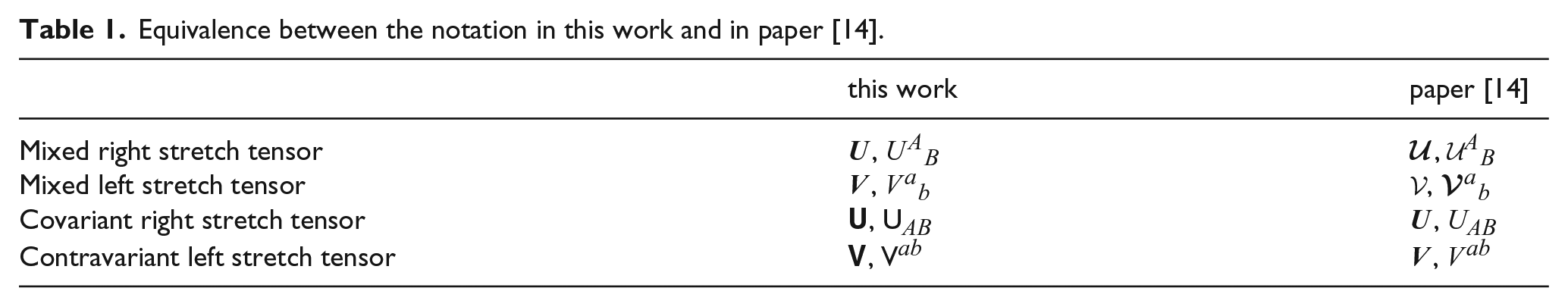
Remark 3. In paper [14], which was written about 10 years ago, the mixed right and left Cauchy–Green deformation tensors with components ${U^A}_B$ and ${V^a}_b$ were denoted by the symbols $\mathcal{U}$ and $\mathcal{V}$ , in calligraphic typeface. This was because the intention was to reserve the symbols $\mathit{U}$ and $\mathit{V}$ to the covariant and contravariant stretch tensors with components $G_{\mathrm{AB}}{U^B}_C$ and ${V^a}_b{g}^{\mathrm{bc}}$ . While there were some advantages in considering these covariant and contravariant stretch tensors as the “standard” ones, the little more maturity gained in the last 10 years suggests that it is wiser to exclusively define $\mathit{U}$ and $\mathit{V}$ as mixed tensors, as they arise from the Polar Decomposition Theorem written in the form (29). So, in order to avoid confusion, whenever it will be necessary to refer to results in paper [14], we shall use a sans serif typeface for the covariant and contravariant stretch tensors

$$\mathsf{U}=\mathit{G}\mathit{U},{\mathsf{U}}_{\mathrm{AC}}=G_{\mathrm{AB}}{U^B}_C,$$

(34a)

$$\mathsf{V}=\mathit{V}{\mathit{g}}^{-1},{\mathsf{V}}^{\mathrm{ac}}={V^a}_b{g}^{\mathrm{bc}}.$$

(34b)

The equivalence with the notation in paper [14] is illustrated in Table 1.

Table 1.

Equivalence between the notation in this work and in paper [14].

	this work	paper [14]
Mixed right stretch tensor	$\mathit{U}$ , ${U^A}_B$	$\mathcal{U}$ , ${{\mathcal{U}}^A}_B$
Mixed left stretch tensor	$\mathit{V}$ , ${V^a}_b$	$\mathcal{V}$ , ${{\mathcal{V}}^a}_b$
Covariant right stretch tensor	$\mathsf{U}$ , ${\mathsf{U}}_{\mathrm{AB}}$	$\mathit{U}$ , $U_{\mathrm{AB}}$
Contravariant left stretch tensor	$\mathsf{V}$ , ${\mathsf{V}}^{\mathrm{ab}}$	$\mathit{V}$ , $V^{\mathrm{ab}}$

2.4. Spectral and pseudo-spectral decompositions

As a corollary of the Polar Decomposition Theorem, we have that $\mathit{U}$ and $\mathit{V}$ are similar tensors, i.e., they are obtained from each other by rotating through $\mathit{R}$ :

$$\mathit{U}(X)={\mathit{R}}^t(x)\mathit{V}(x)\mathit{R}(X),{U^A}_Q(X)=G^{\mathrm{AB}}(X){({\mathit{R}}^T{)}_B}^c(x)g_{\mathrm{cd}}(x){V^d}_p(x){R^p}_Q(X),$$

(35a)

$$\mathit{V}(x)=\mathit{R}(X)\mathit{U}(X){\mathit{R}}^t(x),{V^a}_q(x)={R^a}_B(X){U^B}_C(X)G^{\mathrm{CD}}(X){({\mathit{R}}^T{)}_D}^p(x)g_{\mathrm{pq}}(x).$$

(35b)

This implies that $\mathit{U}$ and $\mathit{V}$ share the same eigenvalues ${\lambda }_{\alpha }$ , called principal stretches, and their eigenvectors, the material principal directions of stretch ${\mathit{N}}_{\alpha }$ and the spatial principal directions of stretch ${\mathit{n}}_{\alpha }$ , are again related through $\mathit{R}$ :

$${\mathit{N}}_{\alpha }(X)={\mathit{R}}^t(x){\mathit{n}}_{\alpha }(x),N_{\alpha }^A(X)=G^{\mathrm{AB}}(X){({\mathit{R}}^T{)}_B}^c(x)g_{\mathrm{cd}}(x)n_{\alpha }^d(x),$$

(36a)

$${\mathit{n}}_{\alpha }(x)=\mathit{R}(X){\mathit{N}}_{\alpha }(X),n_{\alpha }^a(x)={R^a}_B(X)N_{\alpha }^B(X).$$

(36b)

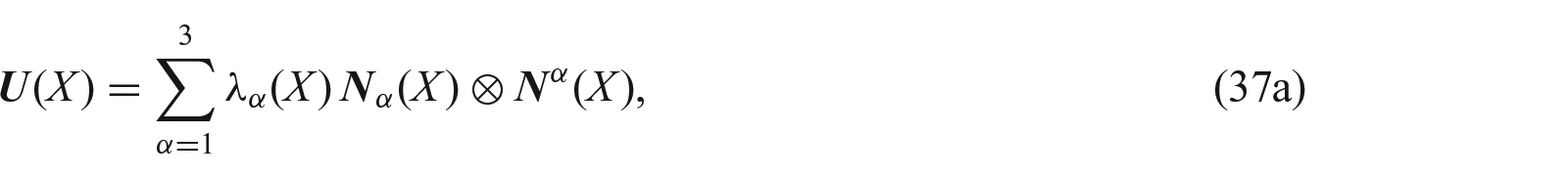
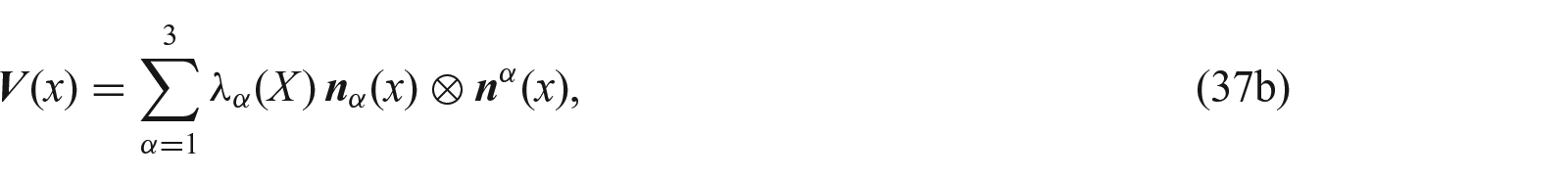
The stretch tensors admit the spectral decompositions

$$\mathit{U}(X)=\sum _{\alpha =1}^3{\lambda }_{\alpha }(X){\mathit{N}}_{\alpha }(X)\otimes {\mathit{N}}^{\alpha }(X),$$

(37a)

$$\mathit{V}(x)=\sum _{\alpha =1}^3{\lambda }_{\alpha }(X){\mathit{n}}_{\alpha }(x)\otimes {\mathit{n}}^{\alpha }(x),$$

(37b)

where

$${\mathit{N}}^{\alpha }(X)=\mathit{G}(X){\mathit{N}}_{\alpha }(X),$$

(38a)

$${\mathit{n}}^{\alpha }(x)=\mathit{g}(x){\mathit{n}}_{\alpha }(x),$$

(38b)

are the covectors associated with ${\mathit{N}}_{\alpha }$ and ${\mathit{n}}_{\alpha }$ through the material and spatial metric tensors $\mathit{G}$ and $\mathit{g}$ .

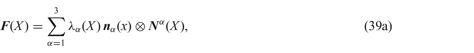
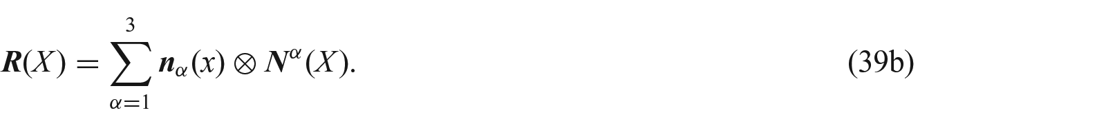
Through the spectral decompositions (37) and the main statement (29) of the Polar Decomposition Theorem, we also obtain the pseudo-spectral decompositions of $\mathit{F}$ and $\mathit{R}$ , as

$$\mathit{F}(X)=\sum _{\alpha =1}^3{\lambda }_{\alpha }(X){\mathit{n}}_{\alpha }(x)\otimes {\mathit{N}}^{\alpha }(X),$$

(39a)

$$\mathit{R}(X)=\sum _{\alpha =1}^3{\mathit{n}}_{\alpha }(x)\otimes {\mathit{N}}^{\alpha }(X).$$

(39b)

2.5. Fundamental deformation tensors

The fundamental deformation tensors are given by the pull-back of the spatial metric tensor $\mathit{g}$ and its inverse ${\mathit{g}}^{-1}$ and the push-forward of the material metric tensor $\mathit{G}$ and its inverse ${\mathit{G}}^{-1}$ [13]. These are the right Cauchy–Green deformation $\mathit{C}$ , its inverse the Piola deformation $\mathit{B}={\mathit{C}}^{-1}$ , the Finger deformation $\mathit{c}$ and its inverse the left Cauchy–Green deformation $\mathit{b}={\mathit{c}}^{-1}$ , and are given by

$$\mathit{C}(X)={\mathit{F}}^T(x)\mathit{g}(x)\mathit{F}(X),C_{\mathrm{AB}}(X)=({\mathit{F}}^T{{)}_A}^a(x)g_{\mathrm{ab}}(x){F^b}_B(X),$$

(40a)

$$\mathit{B}(X)={\mathit{F}}^{-1}(x){\mathit{g}}^{-1}(x){\mathit{F}}^{-T}(X),B^{\mathrm{AB}}(X)=({\mathit{F}}^{-1}{{)}^A}_a(x)g^{\mathrm{ab}}(x){({\mathit{F}}^{-T}{)}_b}^B(X),$$

(40b)

$$\mathit{c}(x)={\mathit{F}}^{-T}(X)\mathit{G}(X){\mathit{F}}^{-1}(x),c_{\mathrm{ab}}(x)=({\mathit{F}}^{-T}{{)}_a}^A(X)G_{\mathrm{AB}}(X){({\mathit{F}}^{-1}{)}^B}_b(x),$$

(40c)

$$\mathit{b}(x)=\mathit{F}(X){\mathit{G}}^{-1}(X){\mathit{F}}^T(x),b^{\mathrm{ab}}(x)={F^a}_A(X)G^{\mathrm{AB}}(X){({\mathit{F}}^T{)}_B}^a(x).$$

(40d)

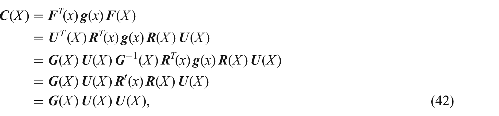
The relation between the deformation tensors (40) and the stretch tensors $\mathit{U}$ and $\mathit{V}$ is found by applying the polar decomposition (29) and exploiting the symmetry conditions (31) for $\mathit{U}$ and $\mathit{V}$ , and the orthogonality condition (30) for $\mathit{R}$ , as

$$\mathit{C}(X)=\mathit{G}(X){\mathit{U}}^2(X),C_{\mathrm{AD}}(X)=G_{\mathrm{AB}}(X){U^B}_C(X){U^C}_D(X),$$

(41a)

$$\mathit{B}(X)={\mathit{U}}^{-2}(X){\mathit{G}}^{-1}(X),B^{\mathrm{AD}}(X)=({\mathit{U}}^{-1}{{)}^A}_B(X){({\mathit{U}}^{-1}{)}^B}_C(X)G^{\mathrm{CD}}(X),$$

(41b)

$$\mathit{c}(x)=\mathit{g}(x){\mathit{V}}^{-2}(x),c_{\mathrm{ad}}(x)=g_{\mathrm{ab}}(x){({\mathit{V}}^{-1}{)}^b}_c(x){({\mathit{V}}^{-1}{)}^c}_d(x),$$

(41c)

$$\mathit{b}(x)={\mathit{V}}^2(x){\mathit{g}}^{-1}(x),b^{\mathrm{ad}}(x)={V^a}_b(x){V^b}_c(x)g^{\mathrm{cd}}(x).$$

(41d)

For instance, the expression (41a) of the right Cauchy–Green deformation tensor is found as

$$\begin{array}{c}\mathit{C}(X)={\mathit{F}}^T(x)\mathit{g}(x)\mathit{F}(X)\hfill \\ ={\mathit{U}}^T(X){\mathit{R}}^T(x)\mathit{g}(x)\mathit{R}(X)\mathit{U}(X)\hfill \\ =\mathit{G}(X)\mathit{U}(X){\mathit{G}}^{-1}(X){\mathit{R}}^T(x)\mathit{g}(x)\mathit{R}(X)\mathit{U}(X)\hfill \\ =\mathit{G}(X)\mathit{U}(X){\mathit{R}}^t(x)\mathit{R}(X)\mathit{U}(X)\hfill \\ =\mathit{G}(X)\mathit{U}(X)\mathit{U}(X),\hfill \end{array}$$

(42)

where the orthogonality condition ${\mathit{R}}^t={\mathit{R}}^{-1}$ (equation (30)) implies ${\mathit{R}}^t(x)\mathit{R}(X)=\mathit{I}$ , where $\mathit{I}$ is the material identity tensor.

2.6. Fundamental strain tensors

The fundamental strain tensors are the material Green–Lagrange strain and the spatial Almansi–Euler strain. Both are defined by comparing a deformed metric with an undeformed metric. The Green–Lagrange strain $\mathit{E}(X)$ compares the pull-back metric $\mathit{C}(X)={\mathit{F}}^T(x)\mathit{g}(x)\mathit{F}(X)$ to the material metric $\mathit{G}(X)$ , and the Almansi–Euler strain compares the spatial metric $\mathit{g}(x)$ to the push-forward metric $\mathit{c}(x)={\mathit{F}}^{-T}(X)\mathit{G}(X){\mathit{F}}^{-1}(x)$ , i.e.,

$$\mathit{E}(X)=\frac{1}{2}(\mathit{C}(X)-\mathit{G}(X)),E_{\mathrm{AB}}(X)=\frac{1}{2}(C_{\mathrm{AB}}(X)-G_{\mathrm{AB}}(X)),$$

(43a)

$$\mathit{e}(x)=\frac{1}{2}(\mathit{g}(x)-\mathit{c}(x)),e_{\mathrm{ab}}(x)=\frac{1}{2}(g_{\mathrm{ab}}(x)-c_{\mathrm{ab}}(x)).$$

(43b)

Note that they are defined in such a way that they are obtainable from each other via pull-back and push-forward operations:

$$\mathit{E}(X)={\mathit{F}}^T(x)\mathit{e}(x){\mathit{F}}^{-T}(X),$$

(44a)

$$\mathit{e}(x)={\mathit{F}}^{-T}(X)\mathit{E}(X){\mathit{F}}^T(x).$$

(44b)

We also note that these two fundamental strains are both covariant and that, normally, no contravariant counterparts are considered.

The Green–Lagrange and Almansi–Euler strains can be written in terms of the right and left stretch tensors using equations (41), as

$$\mathit{E}(X)=\frac{1}{2}(\mathit{G}(X){\mathit{U}}^2(X)-\mathit{G}(X)),E_{\mathrm{AD}}(X)=\frac{1}{2}(G_{\mathrm{AB}}(X){U^B}_C(X){U^C}_D(X)-G_{\mathrm{AD}}(X)),$$

(45a)

$$\mathit{e}(x)=\frac{1}{2}(\mathit{g}(x)-\mathit{g}(x){\mathit{V}}^{-2}(x)),e_{\mathrm{ad}}(x)=\frac{1}{2}(g_{\mathrm{ad}}(x)-g_{\mathrm{ab}}(x){({\mathit{V}}^{-1}{)}^b}_c(x){({\mathit{V}}^{-1}{)}^c}_d(x)).$$

(45b)

Alternatively, the metric tensors can be factorised, so that the terms in parentheses are always mixed tensors, i.e.,

$$\mathit{E}(X)=\frac{1}{2}\mathit{G}(X)({\mathit{U}}^2(X)-\mathit{I}),E_{\mathrm{AD}}(X)=\frac{1}{2}{G}_{\mathrm{AB}}(X)({U^B}_C(X){U^C}_D(X)-{{\delta }^B}_D),$$

(46a)

$$\mathit{e}(x)=\frac{1}{2}\mathit{g}(x)(\mathit{i}-{\mathit{V}}^{-2}(x)),e_{\mathrm{ad}}(x)=\frac{1}{2}{g}_{\mathrm{ab}}(x)({{\delta }^b}_d-{({\mathit{V}}^{-1}{)}^b}_c(x){({\mathit{V}}^{-1}{)}^c}_d(x)),$$

(46b)

where $\mathit{I}$ and $\mathit{i}$ are the material identity tensor and spatial identity tensor, respectively.

3. Hill–Ogden generalised strains

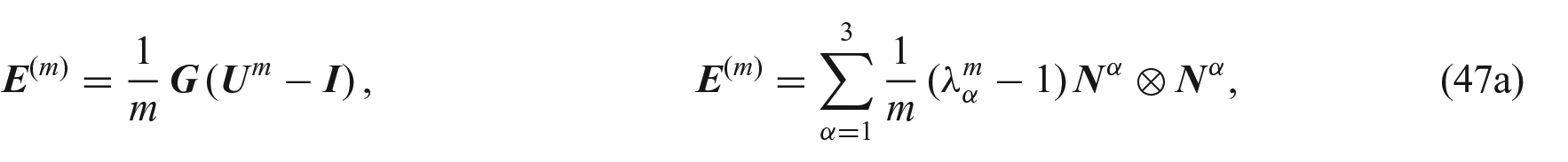
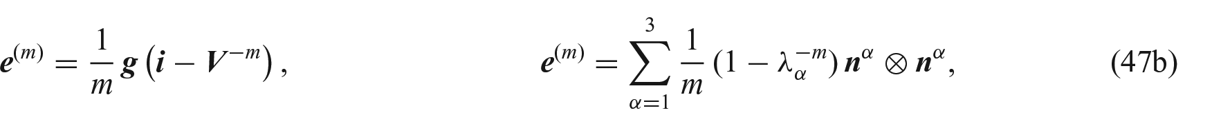
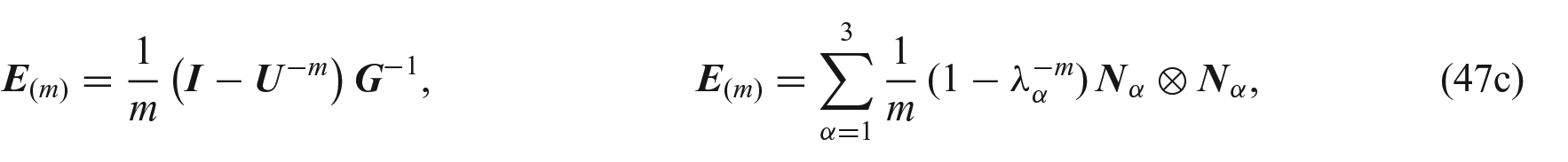
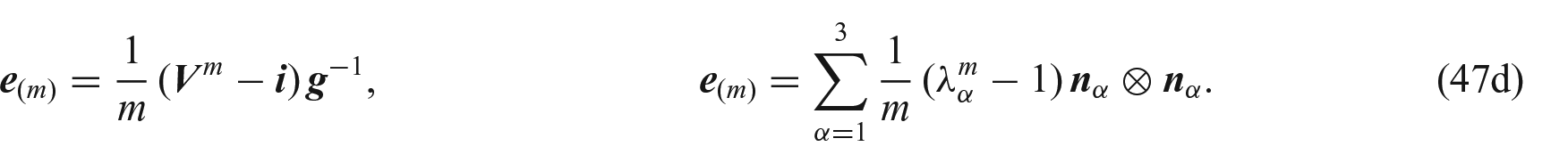
Based on the formalism of section 2.6, we propose to write the Hill–Ogden generalised strain tensors (6) in the form

$${\mathit{E}}^{(m)}=\frac{1}{m}\mathit{G}({\mathit{U}}^m-\mathit{I}),{\mathit{E}}^{(m)}=\sum _{\alpha =1}^3\frac{1}{m}({\lambda }_{\alpha }^m-1){\mathit{N}}^{\alpha }\otimes {\mathit{N}}^{\alpha },$$

(47a)

$${\mathit{e}}^{(m)}=\frac{1}{m}\mathit{g}(\mathit{i}-{\mathit{V}}^{-m}),{\mathit{e}}^{(m)}=\sum _{\alpha =1}^3\frac{1}{m}(1-{\lambda }_{\alpha }^{-m}){\mathit{n}}^{\alpha }\otimes {\mathit{n}}^{\alpha },$$

(47b)

$${\mathit{E}}_{(m)}=\frac{1}{m}(\mathit{I}-{\mathit{U}}^{-m}){\mathit{G}}^{-1},{\mathit{E}}_{(m)}=\sum _{\alpha =1}^3\frac{1}{m}(1-{\lambda }_{\alpha }^{-m}){\mathit{N}}_{\alpha }\otimes {\mathit{N}}_{\alpha },$$

(47c)

$${\mathit{e}}_{(m)}=\frac{1}{m}({\mathit{V}}^m-\mathit{i}){\mathit{g}}^{-1},{\mathit{e}}_{(m)}=\sum _{\alpha =1}^3\frac{1}{m}({\lambda }_{\alpha }^m-1){\mathit{n}}_{\alpha }\otimes {\mathit{n}}_{\alpha }.$$

(47d)

The families (47a) and (47b) are covariant and are constructed on the model of the Green–Lagrange strain $\mathit{E}$ and Almansi–Euler strain $\mathit{e}$ as written in equation (46), i.e., by factorising the metric tensors on the left. The families (47c) and (47d) are instead contravariant and are constructed using the inverse metric tensors, which are factorised on the right. Let us study the covariant and contravariant families in detail.

3.1. Covariant strain families

Defining the strain families (47a) and (47b) as covariant is natural. Indeed, for $m=2$ , they reduce to the Green–Lagrange strain $\mathit{E}$ and the Euler–Almansi strain $\mathit{E}$ written in terms of $\mathit{U}$ and $\mathit{V}$ as in equation (46), with the metric tensors $\mathit{G}$ and $\mathit{g}$ , respectively, factorised on the left. The form (46) can then be transformed back into equation (43), which is written in terms of the right Cauchy–Green deformation $\mathit{C}$ and the Finger deformation $\mathit{c}$ . The two families (47a) and (47b) are often considered to be the only two (e.g., [14,21]).

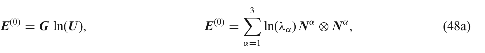
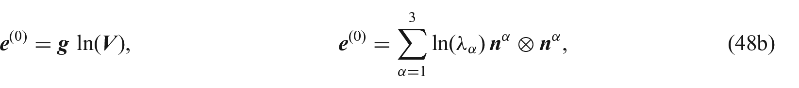
It is worth to look at the logarithmic Hencky strains in detail. The material and spatial logarithmic strains

$${\mathit{E}}^{(0)}=\mathit{G}\ln (\mathit{U}),{\mathit{E}}^{(0)}=\sum _{\alpha =1}^3\ln ({\lambda }_{\alpha }){\mathit{N}}^{\alpha }\otimes {\mathit{N}}^{\alpha },$$

(48a)

$${\mathit{e}}^{(0)}=\mathit{g}\ln (\mathit{V}),{\mathit{e}}^{(0)}=\sum _{\alpha =1}^3\ln ({\lambda }_{\alpha }){\mathit{n}}^{\alpha }\otimes {\mathit{n}}^{\alpha },$$

(48b)

are obtained from equations (47a) and (47b) for $m\to 0$ , by exploiting the fundamental limits (e.g., [14])

$$\underset{m\to 0}{lim}\frac{a^m-1}{m}=\ln (a),\underset{m\to 0}{lim}\frac{1-b^{-m}}{m}=-\ln (b^{-1})=\ln (b),$$

(49)

respectively. The second of the (49) is obtained from the first by changing sign, applying the substitution $a=b^{-1}$ and then applying the identity $-\ln (b^{-1})=\ln (b)$ .

In paper [14], in which we used the contravariant left stretch tensor $\mathsf{V}=\mathit{V}{\mathit{g}}^{-1}$ (see Remark 3), we defined the spatial logarithmic strain as $-\ln ({\mathsf{V}}^{-1})=-\ln ((\mathit{V}{\mathit{g}}^{-1}{)}^{-1})$ . With that definition in mind, in paper [14], we mentioned that applying the identity $-\ln (b^{-1})=\ln (b)$ to $-\ln ({\mathsf{V}}^{-1})$ would be plain wrong, because it would entail a tensor inversion transforming the covariant tensor $-\ln ({\mathsf{V}}^{-1})$ into the contravariant tensor $\ln (\mathsf{V})$ , which clearly cannot be the same.

While this statement was correct, we need to do a mea culpa for Remark 4.3 in paper [14], where we mentioned that writing the spatial Hencky strain with the function $\ln (·)$ rather than with the function $-\ln ((·{)}^{-1})$ was a mistake commonly found in the literature. In fact, this is not a mistake if the Hencky strain is indented as in the definition (48b). To show this, let us consider the limit of equation (47b) for $m\to 0$ . Since the metric tensor can be factorised outside of the limit, the tensor in the limit is mixed, and we have

$${\mathit{e}}^{(0)}=\underset{m\to 0}{lim}\frac{1}{m}\mathit{g}(\mathit{i}-{\mathit{V}}^{-m})=\mathit{g}\underset{m\to 0}{lim}\frac{1}{m}(\mathit{i}-{\mathit{V}}^{-m})=\mathit{g}(-\ln \left({\mathit{V}}^{-1}\right))=\mathit{g}\ln (\mathit{V}).$$

(50)

This is because, since ${\mathit{V}}^{-1}$ is a mixed tensor, its inverse $\mathit{V}$ belongs to the same space as ${\mathit{V}}^{-1}$ . So, more than 10 years after we wrote [14], we realised that, in the literature, the expression $\ln (\mathit{V})$ is simply either the mixed tensor form or the Cartesian form (in which the metric $\mathit{g}$ can safely be omitted) of our ${\mathit{e}}^{(0)}=\mathit{g}\ln (\mathit{V})$ of equation (48b). We felt that this was important to rectify.

3.2. Contravariant strain families

To see why defining the strain families (47c) and (47d) as contravariant is natural, let us look at the strains obtained for $m=2$ . The metric tensors factorised on the right result in the emergence of the Piola deformation tensor $\mathit{B}$ expressed in equation (41b) in terms of ${\mathit{U}}^{-1}$ and of the left Cauchy–Green deformation tensor $\mathit{b}$ expressed in equation (41d) in terms of $\mathit{V}$ . Indeed, we have

$${\mathit{E}}_{(2)}=\frac{1}{2}(\mathit{I}-{\mathit{U}}^{-2}){\mathit{G}}^{-1},{\mathit{E}}_{(2)}=\frac{1}{2}({\mathit{G}}^{-1}-\mathit{B}),$$

(51a)

$${\mathit{e}}_{(2)}=\frac{1}{2}({\mathit{V}}^2-\mathit{i}){\mathit{g}}^{-1},{\mathit{e}}_{(2)}=\frac{1}{2}(\mathit{b}-{\mathit{g}}^{-1}).$$

(51b)

Since the Piola deformation tensor $\mathit{B}$ and the left Cauchy–Green deformation tensor $\mathit{b}$ are the inverses of the right Cauchy–Green deformation tensor $\mathit{C}$ and the Finger deformation tensor $\mathit{c}$ , respectively, the strain tensors ${\mathit{E}}_{(2)}$ and ${\mathit{e}}_{(2)}$ of equation (51) are the most natural contravariant counterparts of the covariant strain tensors ${\mathit{E}}^{(2)}\equiv \mathit{E}$ and ${\mathit{e}}^{(2)}\equiv \mathit{e}$ , i.e., the standard Green–Lagrange and Almansi–Euler strain tensors (43).

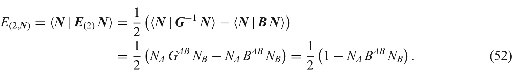
Being contravariant tensors, the tensors ${\mathit{E}}_{(2)}$ and ${\mathit{e}}_{(2)}$ of equation (51) act naturally on covectors, and they take an interesting physical meaning when they act on the covectors normal to surface elements. Let us take the case of the material contravariant strain tensor ${\mathit{E}}_{(2)}$ as an example. To obtain the scalar strain in the direction of the material unit covector $\mathit{N}$ , we write

$$\begin{array}{c}{\mathit{E}}_{(2,N)}=〈\mathit{N}|{\mathit{E}}_{(2)}\mathit{N}〉=\frac{1}{2}(〈\mathit{N}|{\mathit{G}}^{-1}\mathit{N}〉-〈\mathit{N}|\mathit{B}\mathit{N}〉)\hfill \\ =\frac{1}{2}(N_A{G}^{\mathrm{AB}}{N}_B-N_A{B}^{\mathrm{AB}}{N}_B)=\frac{1}{2}(1-N_A{B}^{\mathrm{AB}}{N}_B).\hfill \end{array}$$

(52)

In equation (52), $〈\mathit{N}|{\mathit{G}}^{-1}\mathit{N}〉=N_A{G}^{\mathrm{AB}}{N}_B=\parallel \mathit{N}\parallel =1$ is the norm of $\mathit{N}$ , which is equal to one by hypothesis, while

$$〈\mathit{N}|\mathit{B}\mathit{N}〉=N_A{G}^{\mathrm{AB}}{N}_B\equiv \mathit{B}:(\mathit{N}\otimes \mathit{N})\equiv {\mathit{C}}^{-1}:(\mathit{N}\otimes \mathit{N})$$

(53)

is related to the transversely isotropic invariant $I_5$ , as shown by Merodio and Ogden [11]. We recall that there are five invariants for transverse isotropy: the first three are those for isotropy and the additional two depend on the structure tensor $\mathit{M}\otimes \mathit{M}$ , where the unit vector $\mathit{M}$ is the direction of symmetry of transverse isotropy. The expressions of the invariants are (in our notation)

$$I_1(\mathit{C})={\mathit{G}}^{-1}:\mathit{C},$$

(54a)

$$I_2(\mathit{C})=\frac{1}{2}[({\mathit{G}}^{-1}:\mathit{C}{)}^2-{\mathit{G}}^{-1}:{\mathit{C}}^2],$$

(54b)

$$I_3(\mathit{C})=det(\mathit{C}),$$

(54c)

$$I_4(\mathit{C})=\mathit{C}:(\mathit{M}\otimes \mathit{M}),$$

(54d)

$$I_5(\mathit{C})={\mathit{C}}^2:(\mathit{M}\otimes \mathit{M}),$$

(54e)

where ${\mathit{G}}^{-1}:\mathit{C}$ is the trace of $\mathit{C}$ [22], ${\mathit{C}}^2\equiv \mathit{C}{\mathit{G}}^{-1}\mathit{C}$ defines the square of $\mathit{C}$ , and $det(\mathit{C})\equiv det({\mathit{G}}^{-1}\mathit{C})$ [14]. Via the Hamilton–Cayley Theorem, which, applied to the right Cauchy–Green deformation tensor $\mathit{C}$ , states that $\mathit{C}$ is a root of its characteristic equation $det(\mathit{C}-{\lambda }^2\mathit{G})=0$ (see Appendix 1 in Maleki et al. [23] for a discussion on the eigenvalue problem for covariant tensors), Merodio and Ogden [11] showed that the invariant $I_5$ can be written (in our notation) as

$$I_5(\mathit{C})=I_1(\mathit{C})I_4(\mathit{C})-I_2(\mathit{C})+I_3(\mathit{C})[{\mathit{C}}^{-1}:(\mathit{N}\otimes \mathit{N})],$$

(55)

where $\mathit{N}=\mathit{G}\mathit{M}$ is the material covector associated with the material vector $\mathit{M}$ through the material metric $\mathit{G}$ and

$$I_3(\mathit{C}){\mathit{C}}^{-1}=(det\mathit{C}){\mathit{C}}^{-1}$$

(56)

is the adjoint (or adjugate) of $\mathit{C}$ . Since $I_3(\mathit{C})={\mathit{J}}^2=(det\mathit{F}{)}^2$ , and $\mathit{B}={\mathit{C}}^{-1}={\mathit{F}}^{-1}{\mathit{g}}^{-1}{\mathit{F}}^{-T}$ , it is a simple exercise to show that the last term in equation (55) is the squared norm

$$I_3(\mathit{C})[{\mathit{C}}^{-1}:(\mathit{N}\otimes \mathit{N})]=\parallel J{\mathit{F}}^{-T}\mathit{N}{\parallel }^2$$

(57)

of the covector $J{\mathit{F}}^{-T}\mathit{N}$ , arising from the application of Nanson’s formula to transform the material area element with normal covector $\mathit{N}$ . This observation justifies the definition of the strain families (47c) and (47d) as contravariant tensors.

4. Summary

This work focussed on the Hill–Ogden generalised strains, i.e., the material and spatial Hill [9] strains (3) for which the function $f$ with the properties (4), has either form $\lambda \mapsto \frac{1}{m}({\lambda }^m-1)$ or $\lambda \mapsto \frac{1}{m}(1-{\lambda }^{-m})$ proposed by Ogden [10], as shown in equation (5). Within a fully covariant formalism, we showed how the four families of strains (47) can be grouped into two macro-families.

One macro-family contains the strain tensors that are most naturally defined as being covariant: the material ones (47a) are constructed with the right stretch tensor $\mathit{U}$ and by setting $f:\lambda \mapsto \frac{1}{m}({\lambda }^m-1)$ , and the spatial ones (47b) are constructed with the left stretch tensor $\mathit{V}$ and by setting $f:\lambda \mapsto \frac{1}{m}(1-{\lambda }^{-m})$ . The strain tensors in these two families could be considered as “standard” strain tensors, in so far as they are covariant. Moreover, they contain, as particular cases, the most common measures of strain. The covariant material family (47a) yields the Green–Lagrange strain $\mathit{E}\equiv {\mathit{E}}^{(2)}=\frac{1}{2}\mathit{G}({\mathit{U}}^2-\mathit{I})$ , the Biot strain ${\mathit{E}}^{(1)}=\mathit{G}(\mathit{U}-\mathit{I})$ , and the material Hencky strain ${\mathit{E}}^{(0)}=\mathit{G}\ln (\mathit{U})$ for $m=2$ , $m=1$ and $m\to 0$ , respectively. The covariant spatial family (47b) yields the Almansi–Euler strain $\mathit{e}\equiv {\mathit{e}}^{(2)}=\frac{1}{2}\mathit{g}(\mathit{i}-{\mathit{V}}^{-2})$ and the spatial Hencky strain ${\mathit{e}}^{(0)}=\mathit{g}\ln (\mathit{V})$ for $m=2$ and $m\to 0$ , respectively.

The other macro-family contains the strain tensors that are most naturally defined as being contravariant, and they are constructed by switching the form of the function $f$ with respect to the covariant macro-family: the material ones (47c) are constructed with the right stretch tensor $\mathit{U}$ and by setting $f:\lambda \mapsto \frac{1}{m}(1-{\lambda }^{-m})$ , and the spatial ones (47d) are constructed with the left stretch tensor $\mathit{V}$ and by setting $f:\lambda \mapsto \frac{1}{m}({\lambda }^m-1)$ . The strain tensors in these two families are “non-standard” precisely in so far as they are contravariant. Contravariant strain tensors evaluate the strain along covectors (as opposed to vectors for the case of covariant strain tensors) and thus are suited to evaluate the strain relative to the normal covectors to area elements. For $m=2$ , the material strain tensor is ${\mathit{E}}_{(2)}=\frac{1}{2}(\mathit{I}-{\mathit{U}}^{-2}){\mathit{G}}^{-1}$ and features the Piola deformation tensor $\mathit{B}={\mathit{U}}^{-2}{\mathit{G}}^{-1}$ , while the spatial strain tensor is ${\mathit{e}}_{(2)}=\frac{1}{2}({\mathit{V}}^2-\mathit{i}){\mathit{g}}^{-1}$ and features the left Cauchy–Green deformation tensor $\mathit{b}={\mathit{V}}^2{\mathit{g}}^{-1}$ .

With a didactical intent, this work has attempted to clarify some aspects of the mathematical structure and properties of the Hill–Ogden strain tensors. The covariant formalism facilitates a rigorous presentation of the relation between the stretch tensors $\mathit{U}$ and $\mathit{V}$ and the strain tensors of the four families (47). The hope is that this formalism may be adopted more often in the classroom, at the graduate level, and may perhaps be hinted to also at the undergraduate level.

Dedication

This work is dedicated to Professor Raymond W. Ogden to celebrate his fundamental contributions to the Theory of Elasticity and Continuum Mechanics, on occasion of his 80th birthday. Professor Ogden has had a profound influence on my formation as a theoretical mechanist, both indirectly, through his classical treatise on non-linear elasticity [10], and directly, during his visits to the University of Calgary in 2006 and 2009, and the many discussions that I was fortunate to be able to entertain with him through the years. Grazie, Ray.