Sage Journals: Discover world-class research

Abstract

The inverse finite element method (iFEM) is a powerful tool for shape sensing and structural health monitoring and has several advantages with respect to some other existing approaches. In this study, a two-dimensional four-node quadrilateral inverse finite element formulation is presented. The element is suitable for thin structures under in-plane loading conditions. To validate the accuracy and demonstrate the capability of the inverse element, four different numerical cases are considered for different loading and boundary conditions. iFEM analysis results are compared with regular finite element analysis results as the reference solution, and very good agreement is observed between the two solutions demonstrating the capability of iFEM approach.

Keywords

iFEM shape sensing structural health monitoring quadrilateral two-dimensional

1. Introduction

Structural analysis is an important engineering discipline to ensure the safety of structures. Numerical analysis is widely used for structural analysis calculations based on different approaches ranging from well-known finite element method [1] to semi-analytical approaches [2], higher-gradient theories [3 –6], smoothed particle hydrodynamics (SPH) [7], and more recently peridynamics [8]. Shape sensing and structural health monitoring (SHM) are effective approaches for structural analysis and monitoring. They are mainly based on using sensor systems, collecting sensor data, processing the data, and finally making decisions. Various shape sensing and SHM approaches are available in the literature. One of the most promising approaches is Ko et al.’s [9] displacement theory which is suitable for beam-type structures. As another approach, model method [10] can be used to make predictions without material information. Model method is suitable for both beam- and plate-type structures. As an alternative approach, inverse finite element method (iFEM) [11] can also be used which is the main focus of this study. According to iFEM approach, the solution domain should be discretised with suitable inverse elements (beam, plate, shell, or solid) and strain data from sensors located on different parts of the structure should be collected. It is a robust approach and complex shapes can be monitored in real time. As an additional advantage, loading is not required to be measured during the monitoring process.

Especially during the recent years, there has been a significant progress on iFEM methodology. For different types of structures, different types of inverse elements have been developed. Among these, Tessler and Spangler [12] developed a three-node inverse shell element (iMIN3). iMIN3 is based on the variation of in-plane displacements and bending rotations linearly, and transverse displacements quadratically along with in-plane coordinates. The capability of iMIN3 element has been extended by Tessler et al. [13] for large deformations. An inverse beam element was developed by Gherlone et al. [14] based on Timoshenko beam formulation. A four-node shell element with drilling degree of freedom (iQS4) was introduced by Kefal et al. [15], and iQS4 has been successfully used for monitoring of different marine structures [16], such as chemical tanker [17], containership [18], bulk carrier [19], and offshore wind turbine [20]. Kefal [21] developed an eight-node curved shell element (iCS8) using first-order deformation theory. de Mooij et al. [22] presented a novel inverse solid element formulation and considered various benchmark problems. Composite and sandwich structures are also analysed using iFEM [23,24]. Damage in structures can also be predicted using iFEM [25]. Kefal and Oterkus [26] introduced isogeometric iFEM analysis to reduce the number of required sensors for iFEM analysis, which was further explored in some other studies [27,28].

In this study, a two-dimensional four-node quadrilateral inverse finite element formulation is presented. The element is suitable for thin structures under in-plane loading conditions. To validate the accuracy and demonstrate the capability of the inverse element, three different numerical cases are considered by applying different loading and boundary conditions. iFEM analysis results are compared with regular finite element analysis results as the reference solution.

2. Inverse finite element formulation for a two-dimensional four-node quadrilateral element

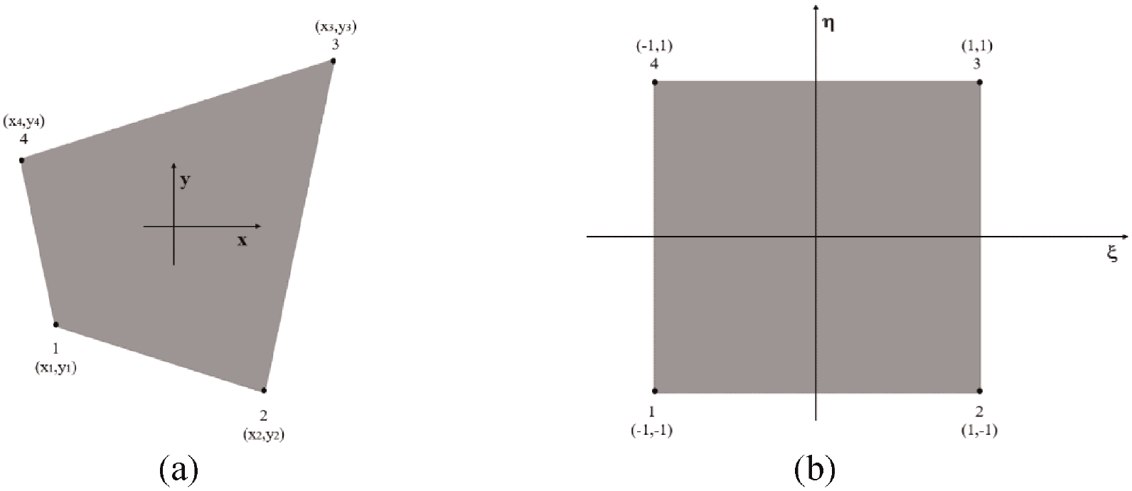
In this section, the details of the formulation for a two-dimensional four-node quadrilateral inverse element, named as iQP4, are provided. As shown in Figure 1(a), each node has two degrees of freedom, $u$ and $v$ , corresponding to in-plane displacements in x- and y-directions, respectively. The master element has a square shape and defined in the natural coordinate system $(ξ, η)$ as depicted in Figure 1(b).

Figure 1.

(a) Two-dimensional four-node quadrilateral inverse element. (b) The master element in $(ξ, η)$ space.

The location of any point on iQP4 element can be expressed in terms of the location of nodes in the $(x, y)$ coordinate system, $(x_{i}, y_{i})$ , and bilinear isoparametric shape functions, $N_{i} (ξ, η)$ as:

x (x, y) = \sum_{i = 1}^{4} N_{i} x_{i},

(1a)

y (x, y) = \sum_{i = 1}^{4} N_{i} y_{i} .

(1b)

The bilinear isoparametric shape functions, $N_{i} (ξ, η)$ , are defined as:

N_{1} = \frac{(1 - ξ) (1 - η)}{4},

(2a)

N_{2} = \frac{(1 + ξ) (1 - η)}{4},

(2b)

N_{3} = \frac{(1 + ξ) (1 + η)}{4},

(2c)

N_{4} = \frac{(1 - ξ) (1 + η)}{4} .

(2d)

Similarly, using the same shape functions, the in-plane displacements, $u$ and $v$ , at any point $(x, y)$ can be written in terms of nodal displacements, $u_{i}$ and $v_{i}$ , as:

u (x, y) = \sum_{i = 1}^{4} N_{i} u_{i},

(3a)

v (x, y) = \sum_{i = 1}^{4} N_{i} v_{i} .

(3b)

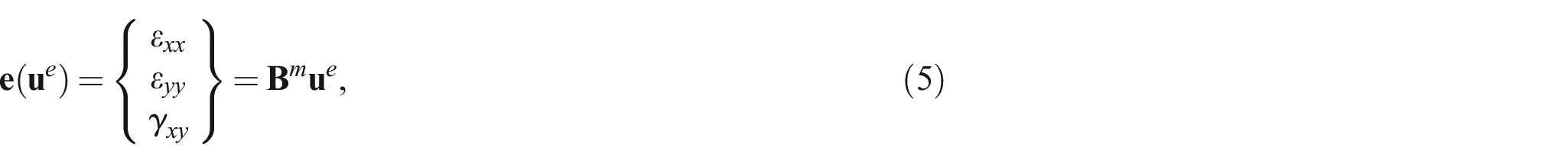
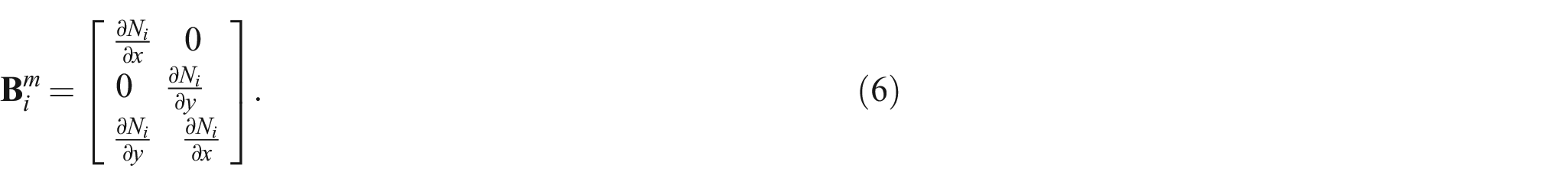
Strain components can be obtained using the relationships between strain and displacement components. For a plane element, only three components of in-plane strains can be expressed as:

ε_{xx} = \frac{\partial u}{\partial x},

(4a)

ε_{yy} = \frac{\partial v}{\partial y},

(4b)

γ_{xy} = \frac{\partial u}{\partial y} + \frac{\partial v}{\partial x} .

(4c)

Using the displacement expressions given in equations (3a) and (3b) and strain definitions given in equations (4a)–(4c), the analytical elemental strains can be expressed by the shape functions and nodal displacements as:

e (u^{e}) = {\begin{matrix} ε_{xx} \\ ε_{yy} \\ γ_{xy} \end{matrix}} = B^{m} u^{e},

(5)

where $u^{e}$ are the nodal displacements, $u^{e} = [\begin{matrix} u_{1} & v_{1} & u_{2} & v_{2} & u_{3} & v_{3} & u_{4} & v_{4} \end{matrix}]^{T}$ . $B^{m}$ is the matrix formed by the shape functions of each node as $B^{m} = [\begin{matrix} B_{1}^{m} & B_{2}^{m} & B_{3}^{m} & B_{4}^{m} \end{matrix}]^{T}$ . Every single $B_{i}^{m}$ matrix can be defined as:

B_{i}^{m} = [\begin{matrix} \begin{matrix} \frac{\partial N_{i}}{\partial x} & 0 \end{matrix} \\ \begin{matrix} 0 & \frac{\partial N_{i}}{\partial y} \end{matrix} \\ \begin{matrix} \frac{\partial N_{i}}{\partial y} & \frac{\partial N_{i}}{\partial x} \end{matrix} \end{matrix}] .

(6)

iFEM solution can be obtained by minimising a weighted least-squares functional with respect to nodal degrees of freedom for the entire solution domain. For each inverse element, the weighted least-squares functional can be written as:

ϕ^{e} (u^{e}) = w_{e} ‖ e (u^{e}) - e^{inputs} ‖^{2},

(7)

where $w_{e}$ is the weighting coefficient and $e^{inputs}$ vector contains the measured strain input data. For real-life applications, measured strains can be obtained from strain sensors, such as strain gauges and fibre optic cables. If the experimental strains for the element are available, then $w_{e} = 1$ . However, if the data are missing, a small value such as $10^{- 3}$ or $10^{- 4}$ would be preferred. The squared norm in equation (7) can be expressed as:

‖ e (u^{e}) - e^{inputs} ‖^{2} = \frac{1}{n} \int \int_{A^{e}} \sum_{i = 1}^{n} {(e {(u^{e})}_{i} - e_{i}^{inputs})}^{2} dxdy,

(8)

where $A_{e}$ is the area of the element and $n$ is the number of locations for measured strains in an element. By minimising the differences between the analytical strains and experimental strains for each element yields,

\frac{\partial ϕ^{e} (u^{e})}{\partial u^{e}} = k^{e} u^{e} - f^{e} = 0,

(9a)

k^{e} u^{e} = f^{e},

(9b)

where $k^{e}$ is the left-hand side matrix and $f^{e}$ is the right-hand side vector generated by the strain inputs which can be, respectively, expressed as:

k^{e} = \int \int_{A^{e}} w_{e} {(B^{m})}^{T} B^{m} dxdy,

(10a)

f^{e} = \frac{1}{n} \int \int_{A^{e}} \sum_{i = 1}^{n} (w_{e} {(B^{m})}^{T} e_{i}^{inputs}) dxdy .

(10b)

Next, the global equation system can be written based on the element contributions given in equations (10a) and (10b) as:

KU = F,

(11)

where

K = \sum_{e = 1}^{Nel} k^{e},

(12a)

F = \sum_{e = 1}^{Nel} f^{e},

(12b)

U = \sum_{e = 1}^{Nel} u^{e},

(12c)

and $Nel$ is the number of inverse elements. After applying displacement boundary conditions, the global equation system will take a reduced form as:

K_{R} U_{R} = F_{R},

(13)

where $K_{R}$ , $U_{R}$ , and $F_{R}$ are reduced global left-hand side matrix, displacement vector, and right-hand side vector. Nodal displacements can be obtained by solution of the equation system given in equation (13). Once the nodal displacements are known, strains and stresses can be obtained similar to the approach used in regular finite element analysis.

3. Numerical examples

We considered four different cases to validate iQP4 inverse plane element formulation and demonstrate its capability, which are listed in Table 1, for different loading and boundary conditions. Furthermore, different mesh configurations together with reduced sensor conditions for fine mesh cases are also taken into consideration.

Table 1.

Description of numerical cases.

Case 1	Square plate under tension with different mesh configurations
Case 2	Rectangular plate under tension with different mesh configurations
Case 3	Square plate with a central hole and fine mesh configuration

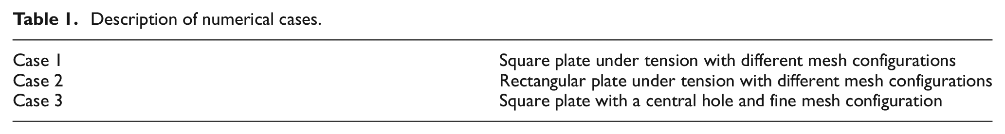
The influence of the mesh size will be explored in Cases 1 and 2. Case 3 is introduced for further verifying the accuracy of iQP4 inverse plane element and sensor selection. The results of displacements in two directions are mainly selected for comparison. For complex structure and loading conditions, von Mises stress is a useful parameter, especially for potential failure of the structure. For the general plane stress condition, the von Mises stress can be calculated as:

σ_{vm} = \sqrt{σ_{xx}^{2} - σ_{xx} σ_{yy} + σ_{yy}^{2} + 3 σ_{xy}^{2}},

(14)

where $σ_{xx}$ , $σ_{yy}$ , and $σ_{xy}$ are in-plane stress components.

3.1. Case 1: square plate under tension loading

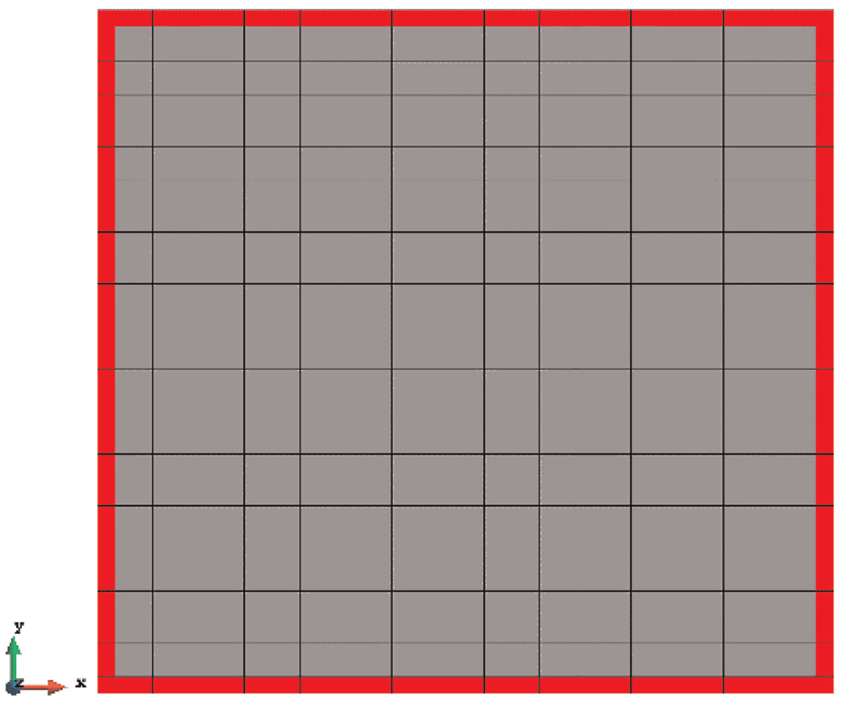
The first case is a square plate (2×2 m²) under tension loading as shown in Figure 2. Moreover, 1000 MN force is evenly distributed to the nodes of each edge of the plate. The plate is meshed with three different numbers of elements which are 16, 100, and 1600, respectively (see Figure 3). The results of the three mesh cases are listed in Tables 2 –4.

Figure 2.

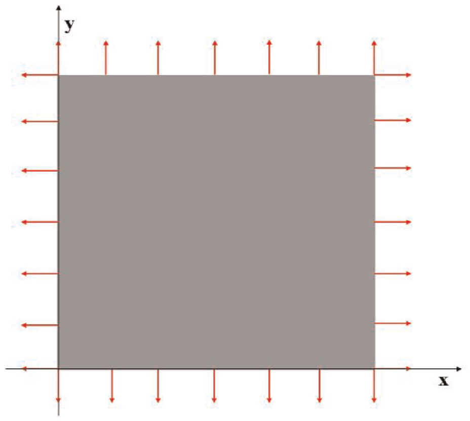
The loading of Case 1.

Figure 3.

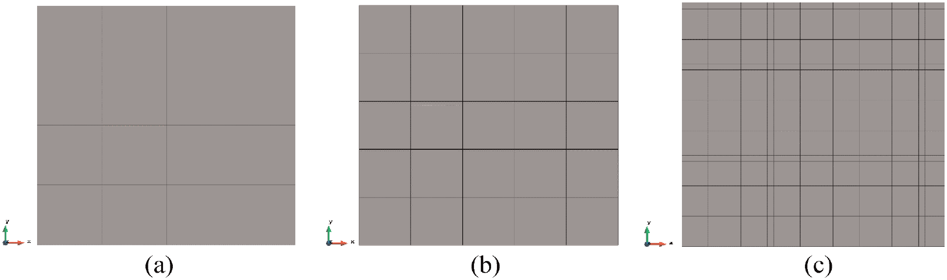
Three different meshes of Case 1. (a) 16 elements. (b) 100 elements. (c) 1600 elements.

Table 2.

The results for Case 1 with 16 elements.

Case 1 with 16 elements		Results
$u$	a. FEM	2.293E−03
	b. iFEM	2.125E−03
Differences between a and b		7.327%
$v$	c. FEM	2.293E−03
	d. iFEM	2.125E−03
Differences between c and d		7.327%

iFEM: inverse finite element method.

Table 3.

The results for Case 1 with 100 elements.

Case 1 with 100 elements		Results
$u$	a. FEM	2.104E−03
	b. iFEM	2.108E−03
Differences between a and b		0.190%
$v$	c. FEM	2.104E−03
	d. iFEM	2.108E−03
Differences between c and d		0.190%

iFEM: inverse finite element method.

Table 4.

The results for Case 1 with 1600 elements.

Case 1 with 1600 elements		Results
$u$	a. FEM	1.847E−03
	b. iFEM	1.823E−03
	c. iFEM-r	1.817E−03
Differences between a and b		1.299%
Differences between a and c		1.624%
$v$	d. FEM	1.847E−03
	e. iFEM	1.823E−03
	f. iFEM-r	1.817E−03
Differences between d and e		1.299%
Differences between d and f		1.624%

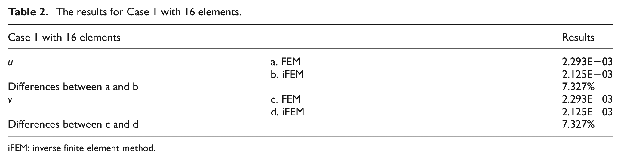
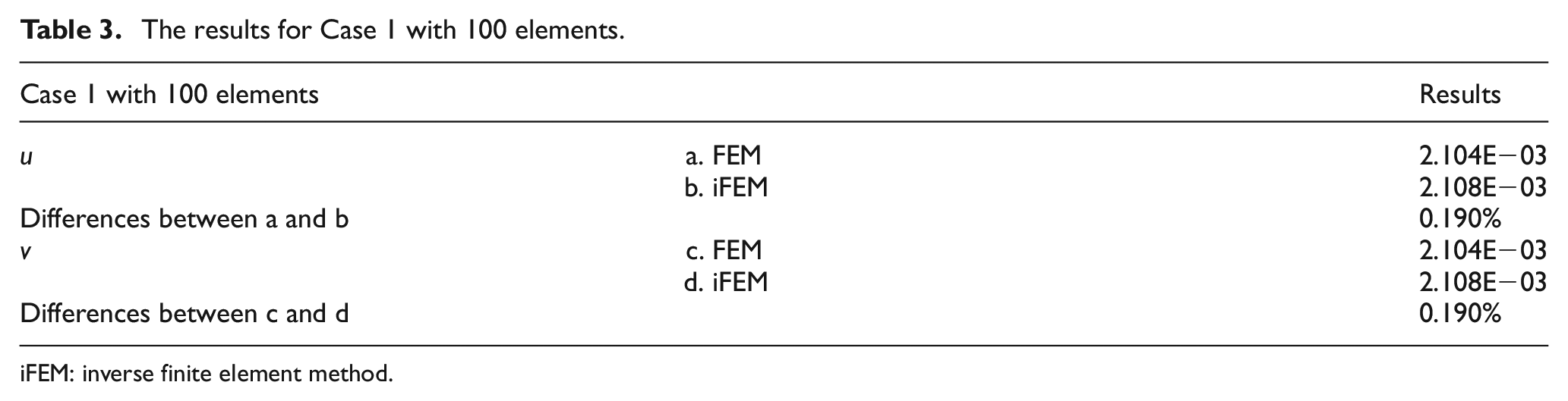
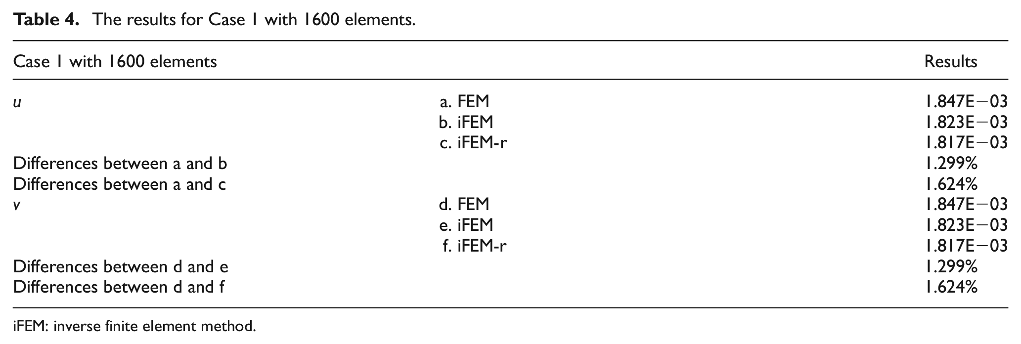
iFEM: inverse finite element method.

For the coarse mesh with 16 elements, as can be seen from Table 2, iFEM displacement results have 7.327% error with respect to FEM results. With the increase in the number of elements, the percentages of difference of displacements are reduced dramatically to 0.190% for 100 elements. For 1600 elements, the reduced sensor condition is applied to the fine mesh case. As shown in Figure 4, only sensors along the edges of the plate are selected which finally gives the number of sensors as 156. With the strain inputs provided by these 156 sensors, even if the strain data for the remaining elements are missing, iQP4 element can still provide accurate results and the percentages of the error just slightly raised from 1.299% to 1.624%.

Figure 4.

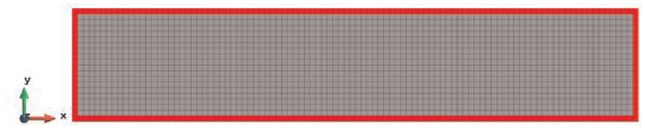
The reduced sensor locations of Case 1 with 1600 elements (iFEM-r).

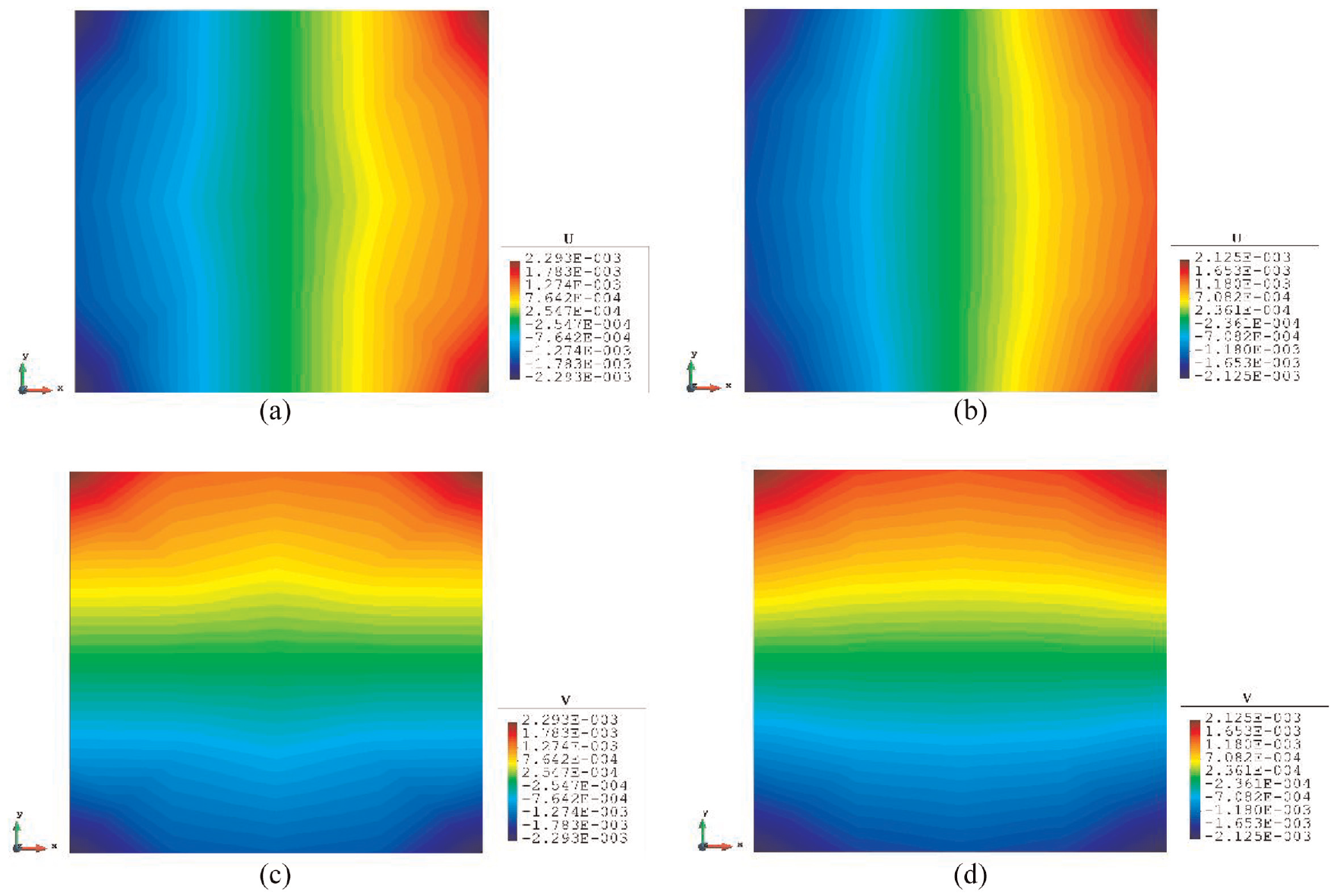
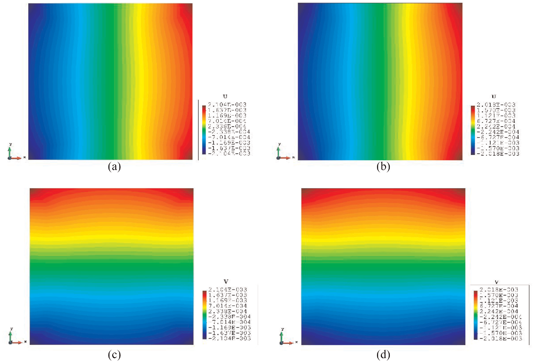
The contour plots of the displacements are also shown in Figures 5 –7 to further illustrate the results. It can be seen that the displacements are symmetrical along the central axis of the plate and the maximum/minimum values appear on the corners of the plate. These typical features can be captured by the inverse analysis, and they are not affected by the mesh and match well with the FEM plots including the reduced sensor condition (iFEM-r).

Figure 5.

The plots of displacements of Case 1 with 16 elements. (a) x-displacements of FEM. (b) x-displacements of iFEM. (c) y-displacements of FEM. (d) y-displacements of iFEM.

Figure 6.

The plots of displacements of Case 1 with 100 elements. (a) x-displacements of FEM. (b) x-displacements of iFEM. (c) y-displacements of FEM. (d) y-displacements of iFEM.

Figure 7.

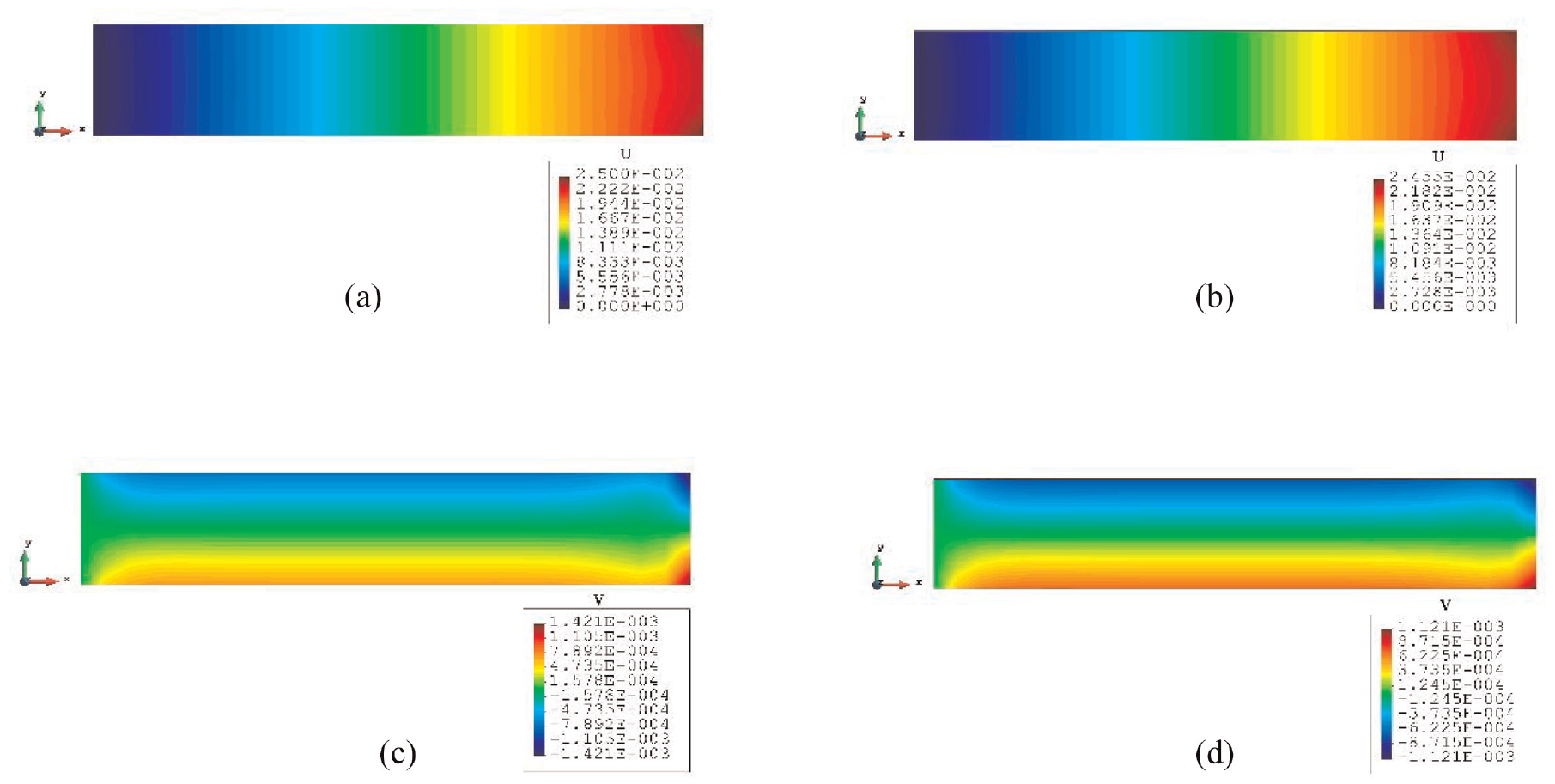
The plots of displacements of Case 1 with 1600 elements. (a) x-displacements of FEM. (b) x-displacements of iFEM. (c) x-displacements of iFEM-r. (d) y-displacements of FEM. (e) y-displacements of iFEM. (f) y-displacements of iFEM-r.

3.2. Case 2: rectangular plate under tension loading

For Case 2, a rectangular plate, with 5 m length and 1 m height, is fully constrained on the left edge and the same tension loading as in Case 1 is applied to the right edge (see Figure 8). Similarly, the plate has been meshed with both coarse mesh (125 elements) and fine mesh (2000 elements) (see Figure 9). Tables 5 and 6 present the results for Case 2. If the mesh is quite coarse, the estimation of the y-displacements is not as good as the x-direction. 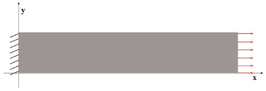The error of the $v$ displacements is about 20% since the displacements in the y-direction are much smaller than the displacements in the x-direction (over 15 times). For the major displacements, $u$ , reasonable results are obtained with an error of 1.800% which means that the results would be acceptable. If the plate is meshed with 2000 elements, the displacements especially in the y-direction are improved. The percentage of the differences is drastically dropped to around or less than 10%, which shows that inverse results are approaching the reference FEM results.

Figure 8.

The loading and displacement boundary conditions of Case 2.

Figure 9.

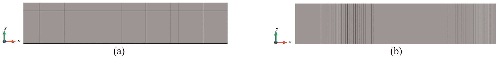
Two different meshes of Case 2. (a) 125 elements. (b) 2000 elements.

Table 5.

The results for Case 2 with 125 elements.

Case 2 with 125 elements		Results
$u$	a. FEM	2.500E−02
	b. iFEM	2.455E−02
Differences between a and b		1.800%
$v$	c. FEM	1.421E−03
	d. iFEM	1.121E−03
Differences between c and d		21.112%

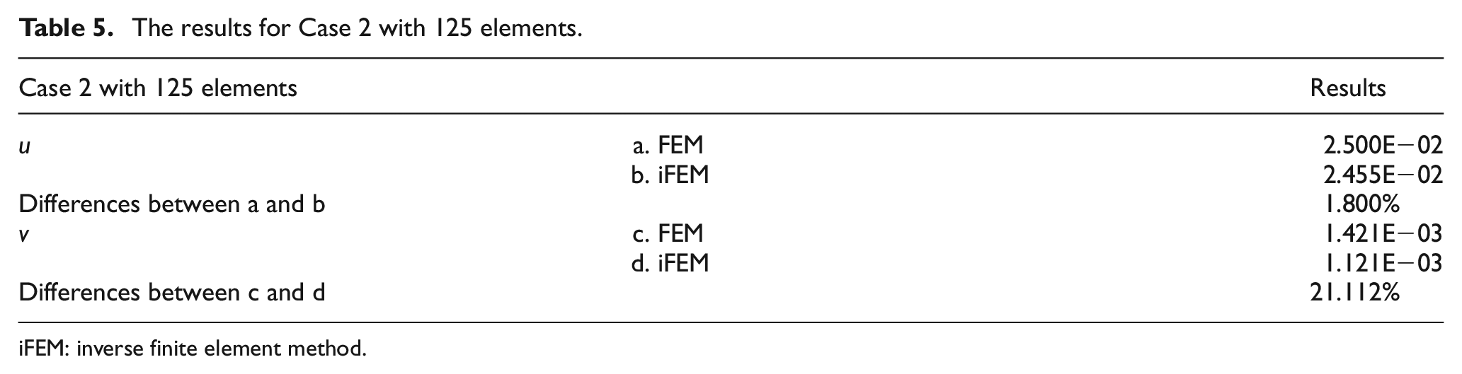
iFEM: inverse finite element method.

Table 6.

The results for Case 2 with 2000 elements.

Case 2 with 2000 elements		Results
$u$	a. FEM	2.444E−02
	b. iFEM	2.431E−02
	c. iFEM-r	2.411E−02
Differences between a and b		0.532%
Differences between a and c		1.350%
$v$	d. FEM	1.127E−03
	e. iFEM	1.039E−03
	f. iFEM-r	1.059E−03
Differences between d and e		7.808%
Differences between d and f		6.034%

iFEM: inverse finite element method.

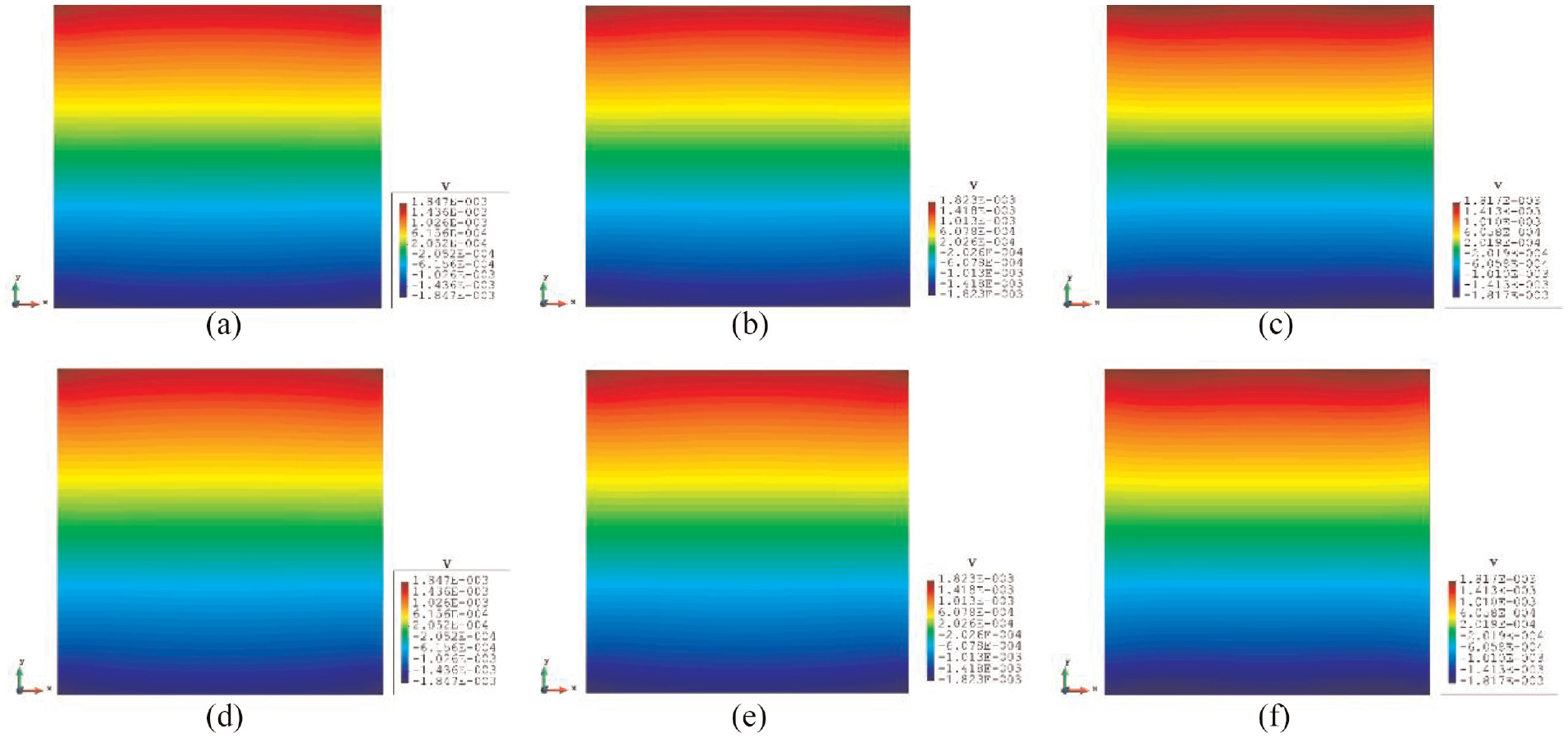
The contour plots of Case 2 are given in Figures 10 and 11. There is no doubt that, for the full sensor condition, the differences of the plots between the inverse analysis and FEM reference are indistinguishable. For the plots of the reduced sensor condition, the sensors are kept along the edge leading to a total number of 236 sensors (Figure 12). Because of the sensor reduction, some features along the edge are not captured clearly. However, the main features, i.e., the locations of the large deformations, are obviously captured.

Figure 10.

The plots of displacements of Case 2 with 125 elements. (a) x-displacements of FEM. (b) x-displacements of iFEM. (c) y-displacements of FEM. (d) y-displacements of iFEM.

Figure 11.

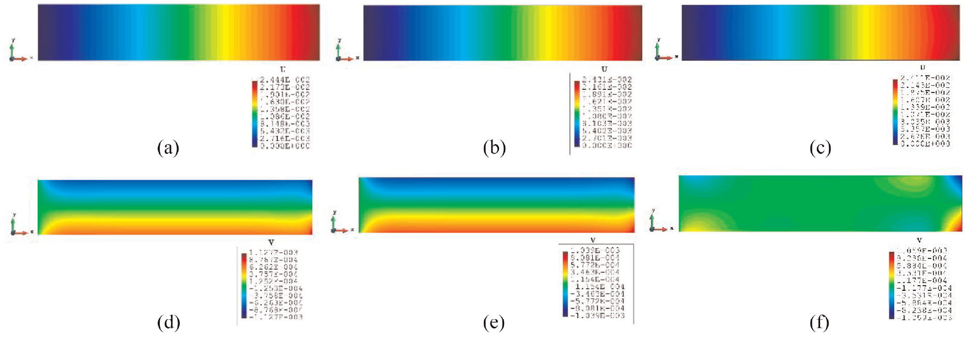
The plots of displacements of Case 2 with 2000 elements. (a) x-displacements of FEM. (b) x-displacements of iFEM. (c) x-displacements of iFEM-r. (d) y-displacements of FEM. (e) y-displacements of iFEM. (f) y-displacements of iFEM-r.

Figure 12.

The sensor locations of Case 2 with 2000 elements.

3.3. Case 3: square plate with a central hole under tension loading

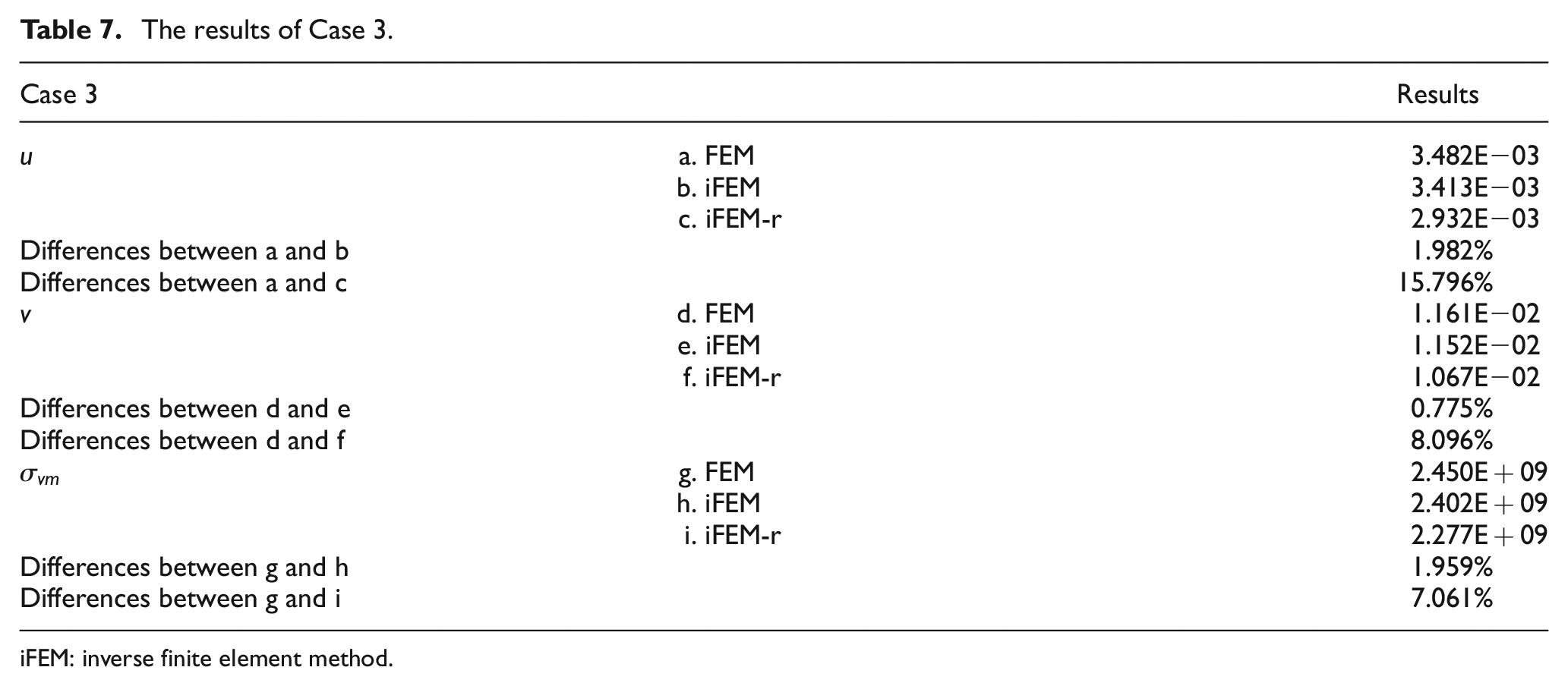
A more complex case which is a plate with a hole at the centre is selected as the last case (Figure 13). The plate has the same geometry as Case 1 and the radius of the hole is 0.5 m. Only dense mesh is considered for Case 3 to ensure the accuracy of FEM analysis, and the plate has been meshed with 1288 elements (Figure 14). The reason for this difference is that around the hole, the mesh would be slightly different, but it will not influence the results. von Mises stress is also chosen for this case to further illustrate the comparison. As shown in Table 7, for the full sensor condition, all three results ( $u$ , $v$ , and $σ_{vm}$ ) for both elements are close to the reference FEM results. For instance, the von Mises stress is 1.959% less than the FEM value for the iQP4 element. Moreover, the number of sensors is reduced to 304 as shown in Figure 15. The current sensor locations can provide less than 10% error for major displacements and von Mises stress. The relatively large percentages of the x-displacements can also be explained by the explanation given in Case 2. For the contour plots of Case 4 (Figures 16 and 17), first of all, the plots of the full sensor condition are almost the same as the FEM plots. The main features and tendencies of the plots are captured by the reduced sensor conditions. For example, from Figure 17(c) and (f), it can be seen that the stress is concentrated around the left and right sides of the central hole, and the minimum stress is located around the bottom of the plate. These characteristics are also presented by the FEM plots. The comparison of the results and figures can prove that iQP4 element even with a limited number of sensors can still estimate accurate results.

Figure 13.

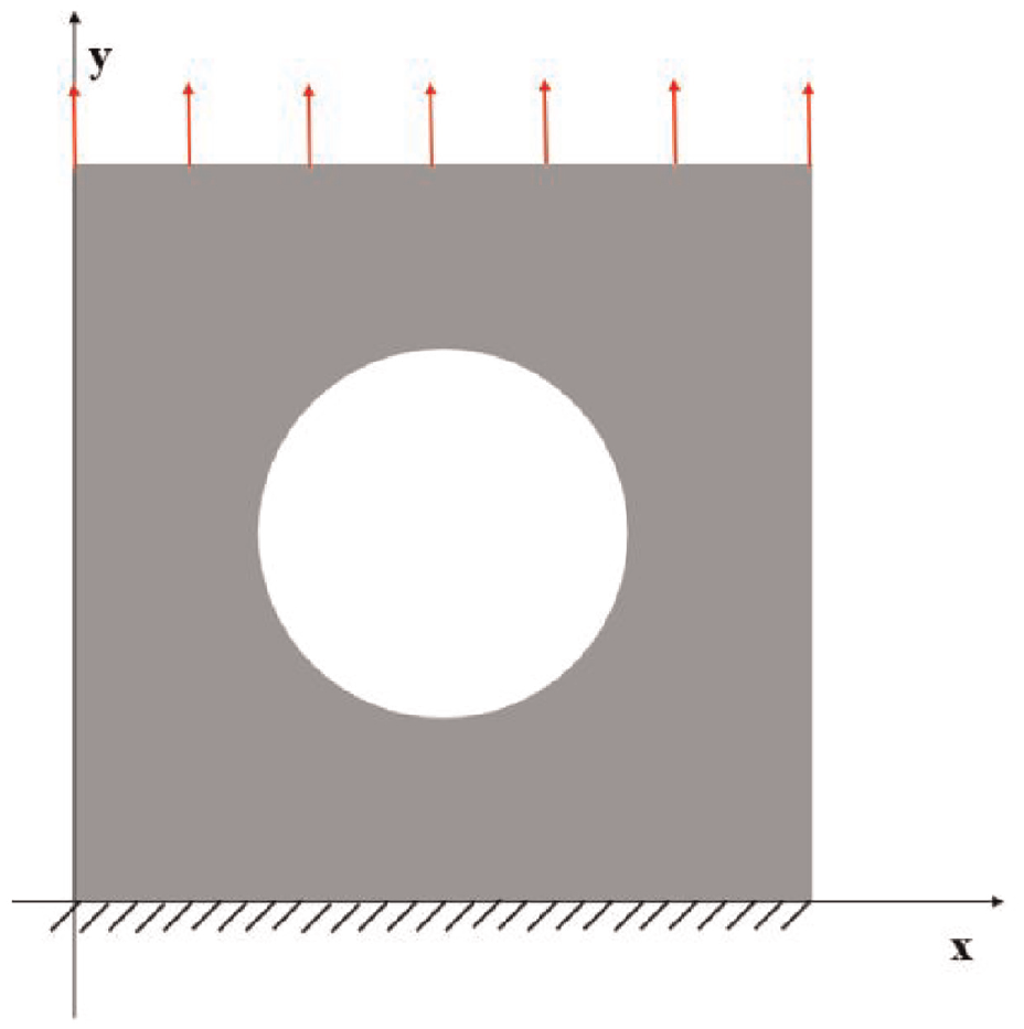
The loading and displacement boundary conditions of Case 3.

Figure 14.

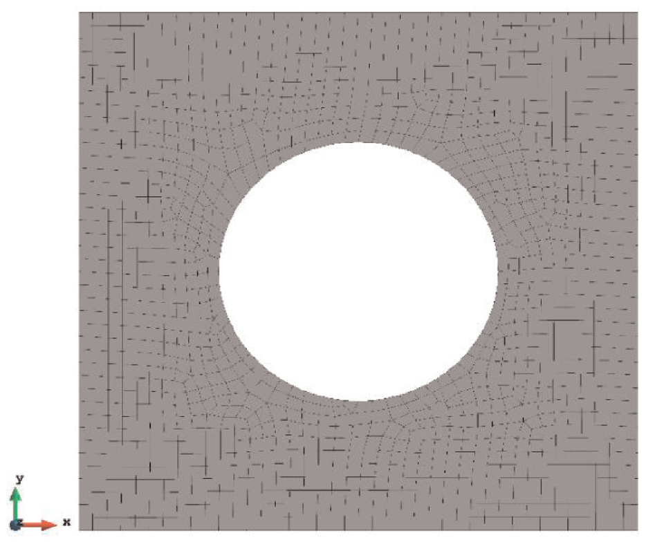
The mesh for Case 3 (1288 elements).

Table 7.

The results of Case 3.

Case 3		Results
$u$	a. FEM	3.482E−03
	b. iFEM	3.413E−03
	c. iFEM-r	2.932E−03
Differences between a and b		1.982%
Differences between a and c		15.796%
$v$	d. FEM	1.161E−02
	e. iFEM	1.152E−02
	f. iFEM-r	1.067E−02
Differences between d and e		0.775%
Differences between d and f		8.096%
$σ_{vm}$	g. FEM	2.450E+09
	h. iFEM	2.402E+09
	i. iFEM-r	2.277E+09
Differences between g and h		1.959%
Differences between g and i		7.061%

iFEM: inverse finite element method.

Figure 15.

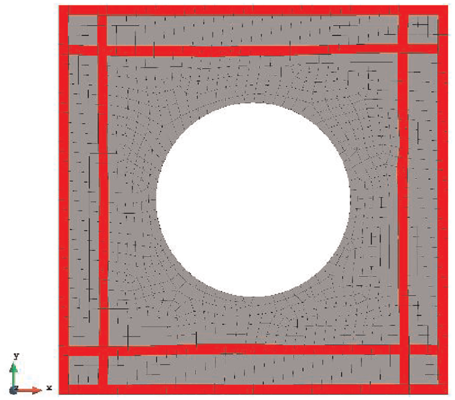
The reduced sensor locations for Case 3 with 1288 elements (iFEM-r).

Figure 16.

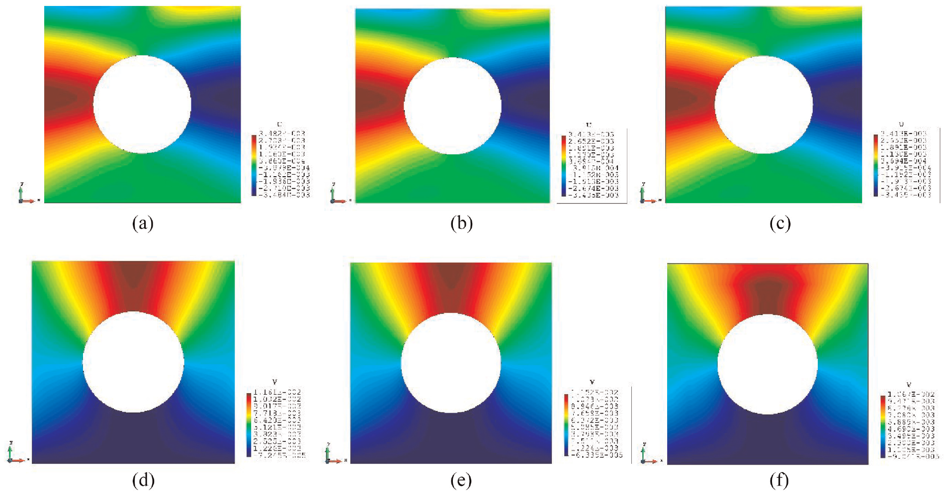
The plots of displacements of Case 3. (a) x-displacements of FEM. (b) x-displacements of iFEM. (c) x-displacements of iFEM-r. (d) y-displacements of FEM. (e) y-displacements of iFEM. (f) y-displacements of iFEM-r.

Figure 17.

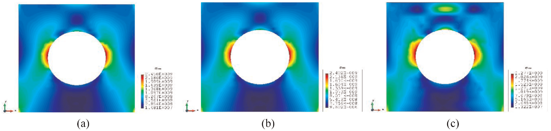
The plots of von Mises stress of Case 3. (a) FEM. (b) iFEM. (c) iFEM-r.

4. Conclusion

In this study, a two-dimensional four-node quadrilateral inverse finite element formulation, iQP4, is presented. To validate the accuracy of the inverse element and demonstrate its capability, four different numerical cases are considered for different loading and boundary conditions. iFEM analysis results are compared with regular finite element analysis results as the reference solution. For all cases, it was demonstrated that iQP4 element can provide accurate results even by considering reduced number of sensors. Therefore, it can be concluded that iFEM and iQP4 element can be used for shape sensing and SHM of structures under in-plane loading conditions.

Footnotes

Funding

The author(s) received no financial support for the research, authorship, and/or publication of this article.

ORCID iD

Erkan Oterkus

References

Zienkiewicz

Taylor

Zhu

. The finite element method: its basis and fundamentals. Amsterdam: Elsevier, 2005.

Oterkus

Madenci

Nemeth

. Stress analysis of composite cylindrical shells with an elliptical cutout. J Mech Mater Struct 2007; 2(4): 695–727.

Alibert

Seppecher

dell’Isola

. Truss modular beams with deformation energy depending on higher displacement gradients. Math Mech Solids 2003; 8(1): 51–73.

Giorgio

Harrison

dell’Isola

, et al. Wrinkling in engineering fabrics: a comparison between two different comprehensive modelling approaches. Proc R Soc A: Math Phys Eng Sci 2018; 474(2216): 20180063.

dell’Isola

Seppecher

Alibert

, et al. Pantographic metamaterials: an example of mathematically driven design and of its technological challenges. Continuum Mech Therm 2019; 31: 851–884.

dell’Isola

Seppecher

Spagnuolo

, et al. Advances in pantographic structures: design, manufacturing, models, experiments and image analyses. Continuum Mech Therm 2019; 31: 1231–1282.

Monaghan

. Smoothed particle hydrodynamics. Annu Rev Astron Astr 1992; 30(1): 543–574.

De Meo

Russo

Oterkus

. Modeling of the onset, propagation, and interaction of multiple cracks generated from corrosion pits by using peridynamics. J Eng Mater Technol 2017; 139(4): 041001.

Richards

Tran

. Displacement theories for in-flight deformed shape predictions of aerospace structures (no. H-2652). Hanover, MD: NASA, 2007.

10.

Bang

Kim

Lee

. Measurement of strain and bending deflection of a wind turbine tower using arrayed FBG sensors. Int J Precis Eng Man 2012; 13(12): 2121–2126.

11.

Tessler

Spangler

. A variational principle for reconstruction of elastic deformations in shear deformable plates and shells (NASA/TM-2003-212445). Hanover, MD: NASA, 2003.

12.

Tessler

Spangler

. Inverse FEM for full-field reconstruction of elastic deformations in shear deformable plates and shells. In: 2nd European workshop on structural health monitoring, Munich, 7–9 July 2004.

13.

Tessler

Spangler

Gherlone

, et al. Deformed shape and stress reconstruction in plate and shell structures undergoing large displacements: application of inverse finite element method using fiber Bragg grating strains. In: Proceedings of 10th world congress on computational mechanics, Sao Paulo, Brazil, 8–13 July 2012.

14.

Gherlone

Cerracchio

Mattone

, et al. Shape sensing of 3D frame structures using an inverse finite element method. Int J Solids Struct 2012; 49(22): 3100–3112.

15.

Kefal

Oterkus

Tessler

, et al. A quadrilateral inverse-shell element with drilling degrees of freedom for shape sensing and structural health monitoring. Eng Sci Technol Int J 2016; 19(3): 1299–1313.

16.

Kefal

Oterkus

. Structural health monitoring of marine structures by using inverse finite element method. In: Soares

Shenoi

(eds) Analysis and design of marine structures V. London: CRC Press, 2015, pp. 341–349.

17.

Kefal

Oterkus

. Displacement and stress monitoring of a chemical tanker based on inverse finite element method. Ocean Eng 2016; 112: 33–46.

18.

Kefal

Oterkus

. Displacement and stress monitoring of a Panamax containership using inverse finite element method. Ocean Eng 2016; 119: 16–29.

19.

Kefal

Mayang

Oterkus

, et al. Three dimensional shape and stress monitoring of bulk carriers based on iFEM methodology. Ocean Eng 2018; 147: 256–267.

20.

Dirik

Oterkus

, et al. Shape sensing of NREL 5 MW offshore wind turbine blade using iFEM methodology. Ocean Eng 2023; 273: 114036.

21.

Kefal

. An efficient curved inverse-shell element for shape sensing and structural health monitoring of cylindrical marine structures. Ocean Eng 2019; 188: 106262.

22.

de Mooij

Martinez

Benedictus

. iFEM benchmark problems for solid elements. Smart Mater Struct 2019; 28(6): 065003.

23.

Cerracchio

Gherlone

Di Sciuva

, et al. A novel approach for displacement and stress monitoring of sandwich structures based on the inverse finite element method. Compos Struct 2015; 127: 69–76.

24.

Kefal

Tessler

Oterkus

. An efficient inverse finite element method for shape and stress sensing of laminated composite and sandwich plates and shells (NASA/TP-2018-220079 (No. L-20938)). Hampton, VA: NASA, 2018.

25.

Colombo

Sbarufatti

Giglio

. Definition of a load adaptive baseline by inverse finite element method for structural damage identification. Mech Syst Signal Process 2019; 120: 584–607.

26.

Kefal

Oterkus

. Isogeometric iFEM analysis of thin shell structures. Sensors 2020; 20(9): 2685.

27.

Zhao

Bao

. An improved inverse finite element method for shape sensing using isogeometric analysis. Measurement 2021; 167: 108282.

28.

Zhao

Bao

, et al. Shape sensing of variable cross-section beam using the inverse finite element method and isogeometric analysis. Measurement 2020; 158: 107656.

A two-dimensional four-node quadrilateral inverse element for shape sensing and structural health monitoring

Abstract

Keywords

1. Introduction

2. Inverse finite element formulation for a two-dimensional four-node quadrilateral element

3. Numerical examples

3.1. Case 1: square plate under tension loading

3.2. Case 2: rectangular plate under tension loading

3.3. Case 3: square plate with a central hole under tension loading

4. Conclusion

Footnotes

Funding

ORCID iD

References