An inverse application of unit cells for extracting fibre properties from effective properties of composites

Abstract

A semi-analytical solution is obtained in this paper for the micromechanical analysis of the square and hexagonal unit cells using complex potentials. It provides a means of numerical characterisation of unidirectionally fibre-reinforced composites for their effective properties. This process is considered as the forward problem and its inverse counterpart is also established in this paper to extract fibre properties from effective properties of composites. It is formulated into a mathematical optimisation problem in which the difference between predicted and provided effective properties is employed as the objective function with the fibre properties as the optimisation variables. The attempt of such an inverse problem is to address the lack of fibre properties for many types of composites commonly in use. The novelty of the paper lies in both sides of the analyses, forward and inverse, as none is available in the literature in the forms as presented in this paper and, more importantly, in the objective of this paper as an attempt to address the pressing and yet long-standing issue of lack of fibre properties. As a verification of the forward analysis, the predicted effective properties of a composite match perfectly with the finite element method (FEM) results. The same case is also employed to verify the inverse analysis by turning the prediction the other way round. Both the forward and inverse analyses have been validated against a series of experimental data. While the forward analysis is generally applicable to any input data as the properties of the constituents, the inverse analysis is sensitive to the input data. Potentially, the inverse analysis would offer a much-needed and also effective tool for the characterisation of fibres. However, reasonable predictions of fibre properties can only be obtained if input data are reasonably consistent.

1. Introduction

One of the acute problems with the design and analysis of composites is the acquisition of a complete and reliable set of fibre properties. The longitudinal Young’s modulus $E_L^f$ and tensile strength are almost all typical manufacturers would provide, for example, TORAY [1] and HEXCEL [2], but more are required usually, namely transverse modulus $E_T^f$ , transverse Poisson’s ratio ${\nu }_T^f$ , and their longitudinal shear modules and Poisson’s ratio $G_L^f$ and ${\nu }_L^f$ . Attempts have been made recently to have them measured experimentally [3], but the techniques employed were quite sophisticated which are not widely accessible to ordinary users and also still yet to be standardised. “Intelligent” guesses or even blindly assumed values have been rather common practices. Typical assumptions were to take the transverse properties, for example, transverse shear modulus G₂₃ or Poisson’s ratio ν₂₃ the same as their longitudinal counterparts G₁₂ or ν₁₂, at least to reduce the number of them. There is absolutely no basis to support this and, in fact, their values are often significantly different. While such assumptions are knowingly far from being satisfactory, yet so often, they are the only option available to many, unfortunately. Some of the best-cited publications in the literature are popular not because of the scientific investigations published there, but because of the relatively complete sets of the material properties provided, in particular, those of the reinforcing fibres. Realistically, it would be a long way ahead before composite designers and analysts would have practical means available to them to have all desired fibre properties experimentally measured beyond manufacturers’ standard provision, such as transverse Young’s modulus and Poisson’s ratio, longitudinal and transverse shear moduli.

It is true that the properties provided by manufacturers are of top significance. They should be sufficient for rough estimates, such as those using netting analysis [4]. As composites are used more and more in engineering, in particular, in aerospace industry where precise predictions of the performances of the composites employed are not only desirable but becoming more and more essential nowadays, the tolerance to put up with rough estimates is shrinking rapidly. This paper intends to put forward a systematic theoretical means to serve the purpose of determining those unavailable elastic properties of fibres, as identified at the beginning of the previous paragraph.

With increasing power and confidence in the characterisation of unidirectional (UD) composites using micromechanics based on unit cells [5,6], it is reasonable to expect an extension of the capability of the use of unit cells can be made. It is in the direction of determination of fibre properties using the bulk properties of the matrix and the effective properties of composites. Mathematically, if the characterisation of composites based on the properties of their constituents is considered as a forward problem, then the desired process can be considered as the inverse problem to its forward counterpart. Since the forward problem is not in any form of closed solution, its inverse counterpart will have to be approximate and numerical in nature, adopting some kind of iterative process. In the literature, most analyses of unit cells have been based on finite element method (FEM) using a commercial FE code typically. It would be rather heavy-handed to incorporate such an analysis into an iterative process, especially when the number of iterations is large. Even if one could, it would be least efficient.

A semi-analytical solution is therefore pursued in this paper for the analysis of appropriate unit cells relevant to UD composites using complex potentials as the solution to the forward problem. Such approach can be validated using FEM. The analyses of unit cells have been carried out using FEM predominantly. Analytical attempts were scarce. An available account can be found in the study by Chen and Cheng [7] but the boundary conditions employed were questionable because no difference was made between symmetric and antisymmetric load cases after the use of reflectional symmetries. The formulations of unit cells started to be taken seriously since the publication of Li [8]. Through subsequent generalisations [9,10], the subject started to take its shape. Eventually, all relevant developments have been systematically delivered in the study by Li and Sitnikova [5,6] in the most comprehensive manner.

Inverse problems are mathematical challenges in general. For almost every physical problem, some kind of inverse problems can be proposed. For a given forward problem, the inverse problems corresponding to it are not unique in general. For a chosen inverse problem, the solution is usually not unique either and, sometimes, it may not even exist, giving its ill-posed nature for inverse problems in general [11]. Examples of formulation of inverse problem in different disciplines of science and engineering can be found in the study by Nanthakumar et al. [11,12], to name but a few, noticing that the study by Nanthakumar et al. [11] was published in a journal dedicated specifically to inverse problems.

The current inverse problem has been formulated into a minimisation problem for the errors of the obtained effective properties of the composite obtained from the forward analysis relative to the provided ones. A mathematical optimiser can be employed to facilitate the iterations. Mathematical optimisation is a reasonably well-established subject. Its maturity can be signified by its presence in mainstream mathematical codes, such as MATLAB [13]. The challenges to users have been reduced to the formulation of the practical problem into an optimisation problem mathematically, which is not always trivial.

In the present optimisation problem, a reasonable approximation of the fibre properties can be achieved once the errors have been minimised. Both of the forward and the inverse processes have been thoroughly verified and validated. It therefore offers a practical means of virtual testing for elastic properties of fibres.

The only account along this line was by the authors in a primitive manner [14]. The problem has now been properly elaborated in this paper. Although the first attempt was so long ago, the demand for such an approach has not diminished over time, as the position of lack of fibre properties stands unchanged.

2. The forward problem: the analysis of a generalised plane strain problem for square and hexagonal unit cells

Before the desired inverse counterpart can be established, its forward problem has to be addressed appropriately and it is presented in this section. It is an analysis of square and hexagonal unit cells under a generalised plane strain (GPE ¹ ) condition [5,6,8,9,15] which is directly applicable to unidirectionally (UD) fibre-reinforced composites. The GPE problem allows the material represented by the unit cells to be subjected to all loading conditions required to characterise the elastic behaviour of such composites. However, for the subsequent use of the analysis in the inverse problem, the analysis will have to be conducted analytically or semi-analytically, away from the conventional FE analysis as dealt with in the study by Li and Sitnikova [5,6], so that it can be incorporated into an iterative optimisation process as the means of solution technique for the inverse problem. With appropriate extension, the forward analysis of unit cells could accommodate certain mechanisms to incorporate the effects of damage, although this is beyond the scope of the present paper.

2.1. Complex function solution of the GPE problem

For the conventional plane strain problem in the cross-section plane transverse to the fibre direction, and the anticlastic problem for the shear deformation along fibres out of the cross-section plane, there have been elegant solutions separately presented in the theory of elasticity employing complex functions [16,17]. The GPE problem represents a slight generalisation by merging both into the same formulation while allowing non-vanishing constant direct strain in the fibre direction [15].

Introduce the coordinate system in such a way that the cross-section of the composite lies in the x-y plane while the fibres run along the z-axis. The coordinate plane x-y coincides with the complex plane on which any point is defined by a complex variable ζ = x + iy. The solution to any GPE problem can be given in terms of three analytic complex functions, φ(ζ), ψ(ζ), and ω(ζ), also called potentials since they are all analytic and hence bear a path-independent characteristic, through which the solution can always be expressed as:

$$\begin{array}{c}{\sigma }_x+{\sigma }_y=4\mathrm{Re}\phi \prime \left(\zeta \right)\hfill \\ {\sigma }_y-{\sigma }_x+2i{\tau }_{\mathrm{xy}}=2(\overline{\zeta }\phi \prime \prime \left(\zeta \right)+\psi \prime \left(\zeta \right))\hfill \\ 2G_T(u+\mathrm{iv})=\kappa \phi \left(\zeta \right)-\zeta \overline{\phi \prime \left(\zeta \right)}-\overline{\psi \left(\zeta \right)}-2G_T{\nu }_L{\epsilon }^0\zeta \hfill \end{array}$$

(1a)

where ${\sigma }_x$ , ${\sigma }_y$ , and ${\tau }_{\mathrm{xy}}$ are the stresses, and u and v are the displacements in the x-y plane, and ${\epsilon }^0$ is the direct strain in the fibre direction which is constant over the cross-section plane [16]; and

$$\begin{array}{c}{\tau }_{\mathrm{xz}}-i{\tau }_{\mathrm{yz}}=\omega \prime (\zeta )\hfill \\ G_{L}w=\mathrm{Re}\omega (\zeta )+G_L{\epsilon }^0\hfill \end{array}$$

(1b)

where ${\tau }_{\mathrm{xz}}$ and ${\tau }_{\mathrm{yz}}$ are the stresses and w is the displacement out of the x-y plane [17]. As a GPE problem, the remaining stress component can always be obtained as follows:

$${\sigma }_z={\nu }_L({\sigma }_x+{\sigma }_y)+E_L{\epsilon }^0.$$

(2)

In equations (1) and (2), E_L, E_T, G_L, G_T, ν_L, and ν_T are the longitudinal and transverse Young’s moduli, shear moduli, and Poisson’s ratios, respectively, where the transverse properties satisfy,

$$G_T=\frac{E_T}{2(1+{\nu }_T)}$$

(3)

as a requirement from transverse isotropy which most UD composites feature;

$$\kappa =-1+\frac{4(1-{\nu }_L^2{E}_T/E_L)}{(1+{\nu }_T)}$$

(4)

is a material constant; $i=\sqrt{-1}$ is the imaginary unity; Re represents the real part of a complex function while the corresponding imaginary part is denoted as Im as will be employed later. In equation (1), the length of the composite in the z-direction has been assumed to be unity. A prime on a function represents its derivative with respect to the complex variable ζ. A bar on the top of a function means its complex conjugate.

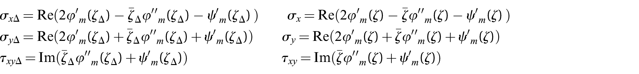
From equation (1), it is straightforward to obtain the individual components of the stresses and displacements and expressed in terms of the three complex potentials as follows:

$$\begin{array}{c}{\sigma }_x=\mathrm{Re}(2\phi \prime (\zeta )-\overline{\zeta }\phi \prime \prime (\zeta )-\psi \prime (\zeta ))\hfill \\ {\sigma }_y=\mathrm{Re}(2\phi \prime (\zeta )+\overline{\zeta }\phi \prime \prime (\zeta )+\psi \prime (\zeta ))\hfill \\ {\tau }_{\mathrm{xy}}=\mathrm{Im}(\overline{\zeta }\phi \prime \prime (\zeta )+\psi \prime (\zeta ))\hfill \end{array}$$

(5a)

$$\begin{array}{c}{\tau }_{\mathrm{xz}}=\mathrm{Re}\omega \prime (\zeta )\hfill \\ {\tau }_{\mathrm{yz}}=-\mathrm{Im}\omega \prime (\zeta )\hfill \end{array}$$

(5b)

in addition to the longitudinal direct stress ${\sigma }_z$ as given in equation (2). The corresponding displacements are:

$$\begin{array}{c}u=\frac{1}{2G_T}\mathrm{Re}(\kappa \phi (\zeta )-\zeta \overline{\phi \prime (\zeta )}-\overline{\psi (\zeta )})-{\nu }_L{\epsilon }^{0}x\hfill \\ v=\frac{1}{2G_T}\mathrm{Im}(\kappa \phi (\zeta )-\zeta \overline{\phi \prime (\zeta )}-\overline{\psi (\zeta )})-{\nu }_L{\epsilon }^{0}y\hfill \end{array}$$

(6a)

$$w=\frac{1}{G_L}\mathrm{Re}\omega (\zeta )+{\epsilon }^0.$$

(6b)

It is now clear that the solution to the GPE problem relies on three complex potentials, with which all governing equations of elasticity are satisfied. All they need to meet are the boundary conditions, including those on the internal boundaries and the external ones.

2.2. Series form of the complex potentials

To model the behaviour of the composites using a unit cell, whether square one or hexagonal one, as shown in Figure 1, there is one fibre involved in each unit cell surrounded by matrix. Thus, there are two regions in the domain, corresponding to the fibre and the matrix, respectively. For simplicity, the problem can always be scaled appropriately, so that the fibre region in the domain is defined as a unit circle centred at the origin of the x-y plane, that is, $\zeta =\rho =e^{i\theta }$ , with θ being the polar angle. Complex functions have to be defined separately within these two distinct regions. While the same notation will be adopted, each will be given a subscript of either f or m representing fibre and matrix, respectively. Solution in a form of series will be pursued below.

Figure 1.

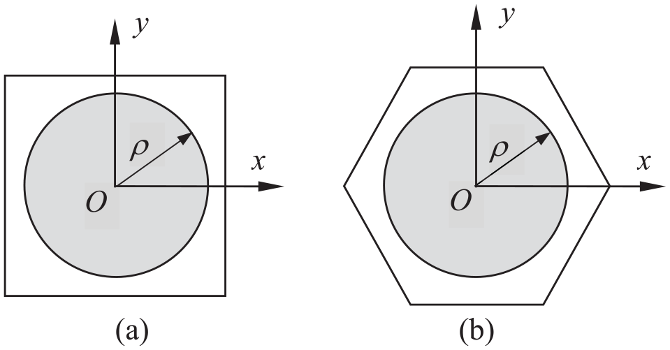
(a) A square unit cell, and (b) a hexagonal unit cell.

The complex potentials for the fibre, that is, defined within the unit circle, are φ_f, ψ_f, and ω_f, expressed in terms of Taylor series as:

$${\phi }_f=\sum _{k=1}^{\infty }{a}_k{\zeta }^k,{\psi }_f=\sum _{k=1}^{\infty }{b}_k{\zeta }^k,\mathrm{and}{\omega }_f=\sum _{k=1}^{\infty }{c}_k{\zeta }^k$$

(7)

where the zeroth-order terms have been dropped as the rigid body displacements are constrained at the origin, that is,

$${u|}_{\zeta =0}={v|}_{\zeta =0}={w|}_{\zeta =0}=0\mathrm{or}{\phi }_f\left(0\right)={\psi }_f\left(0\right)={\omega }_f\left(0\right)=0.$$

(8)

In the matrix region, that is, within the unit cell but outside the unit circle, the complex potentials for the matrix, φ_m, ψ_m, and ω_m, can be expressed in terms of Laurent series as:

$${\phi }_m=\sum _{k=0}^{\infty }{A}_k{\zeta }^k+\sum _{k=1}^{\infty }{D}_k{\zeta }^{-k},{\psi }_m=\sum _{k=0}^{\infty }{B}_k{\zeta }^k+\sum _{k=1}^{\infty }{F}_k{\zeta }^{-k},\mathrm{and}{\omega }_m=\sum _{k=0}^{\infty }{C}_k{\zeta }^k+\sum _{k=1}^{\infty }{H}_k{\zeta }^{-k}.$$

(9)

The rigid body displacements should not be constrained in the matrix directly. Instead, their constraints will be accomplished through the continuity conditions between the fibre and the matrix. For this reason, the zeroth-order terms have been retained in equation (9).

It is well established that Taylor series in a solid domain and Laurent series in a hollow domain as involved in the current problem are both analytic. The validity of the solution can therefore be taken for granted once the coefficients in series (7) and (9) have been correctly determined. Apparently, coefficients a_k, b_k, and c_k in equation (7) are associated with the fibre, and A_k, B_k, C_k, D_k, F_k, and H_k in equation (9) with the matrix. They should be determined by the continuity conditions between fibre and matrix, and the boundary conditions for the unit cell concerned. It will be shown below that those associated with the matrix can be expressed in terms of those associated with the fibre after imposing the continuity conditions between the fibre and the matrix across the interface.

It should be pointed out that, unlike the unit cells analysed using FEM where traction boundary conditions are natural boundary conditions and do not need any attention from users, both displacement boundary conditions and the traction boundary conditions will have to be satisfied simultaneously as the present solution is no longer based on a variational principle.

2.3. Continuity across fibre–matrix interface

It is assumed that perfect bonding is present between the fibre and the matrix. Thus, both the displacements and traction components should be continuous at interface $\zeta =\rho$ . Denote the traction components in the x-y plane as:

$$\begin{array}{c}X={\sigma }_x\cos \beta +{\tau }_{\mathrm{xy}}\sin \beta \hfill \\ Y={\tau }_{\mathrm{xy}}\cos \beta +{\sigma }_y\sin \beta \hfill \end{array}$$

(10)

where β is the angle between the outward normal to the unit circle and the x-axis. They are related to the complex potential functions in general as follows [16]:

$$i\int (X+\mathrm{iY})\mathrm{ds}=\phi (\rho )+\rho \overline{\phi \prime (\rho )}+\overline{\psi (\rho )}$$

(11)

where s is the arc length along the interface. The traction component in the z-direction can be given as [12]:

$$Z={\tau }_{\mathrm{xz}}\cos \beta +{\tau }_{\mathrm{yz}}\sin \beta =\rho \omega \prime (\rho )+\overline{\rho \omega \prime (\rho )}.$$

(12)

The traction continuity conditions between fibre and matrix across the interface can be obtained as:

$$\begin{array}{c}{\phi }_m(\rho )+\rho \overline{{\phi \prime }_m(\rho )}+\overline{{\psi }_m(\rho )}={\phi }_f(\rho )+\rho \overline{{\phi \prime }_f(\rho )}+\overline{{\psi }_f(\rho )}\hfill \\ \rho {\omega \prime }_m(\rho )+\overline{\rho {\omega \prime }_m(\rho )}=\rho {\omega \prime }_f(\rho )+\overline{\rho {\omega \prime }_f(\rho )}.\hfill \end{array}$$

(13a)

Expressing displacement (6) in the fibre and the matrix, respectively, the displacement continuity conditions across the interface are given as:

$$\begin{array}{c}{\kappa }_m{\phi }_m\left(\rho \right)-\rho \overline{{\phi \prime }_m\left(\rho \right)}-\overline{{\psi }_m\left(\rho \right)}=\eta ({\kappa }_f{\phi }_f\left(\rho \right)-\rho \overline{{\phi \prime }_f\left(\rho \right)}-\overline{{\psi }_f\left(\rho \right)})+2G_{\mathrm{Tm}}({\nu }_{\mathrm{Lm}}-{\nu }_{\mathrm{Lf}}){\epsilon }^0\rho \hfill \\ {\omega }_m\left(\rho \right)+\overline{{\omega }_m\left(\rho \right)}=\lambda ({\omega }_f\left(\rho \right)+\overline{{\omega }_f\left(\rho \right)})\hfill \end{array}$$

(13b)

where κ_f and κ_m are the same expression as given in equation (4) but in the fibre and the matrix, respectively

$$\eta =\frac{G_{\mathrm{Tm}}}{G_{\mathrm{Tf}}}\mathrm{and}\lambda =\frac{G_{\mathrm{Lm}}}{G_{\mathrm{Lf}}}.$$

(14)

The term associated with ${\epsilon }^0$ also appears in displacement w. However, it does not show in the second equation of equation (13b) because it appears on both sides of the equation with equal magnitude as it corresponds to the same z-coordinate and therefore is duly cancelled.

Substitute equations (7) and (9) into equation (13), bearing in mind the following equalities from the unit circle:

$$\rho =e^{i\theta },\overline{{\rho }^k}=e^{-\mathrm{ik}\theta }={\left(e^{\mathrm{ik}\theta }\right)}^{-1}={\left({\rho }^k\right)}^{-1}={\rho }^{-k}\mathrm{and}\overline{{\rho }^{-k}}=\overline{e^{-\mathrm{ik}\theta }}=e^{\mathrm{ik}\theta }={\rho }^k$$

(15)

the coefficients A_k, B_k, C_k, D_k, F_k, and H_k in equation (9) can be linearly expressed in terms of a_k, b_k, and c_k in equation (7), after comparing the coefficients to the terms of the same order on both sides of the equations:

$$A_0=\frac{2(1-\eta )}{1+{\kappa }_m}{\overline{a}}_2,A_1=\frac{1}{1+{\kappa }_m}({\overline{a}}_1+a_1-\eta ({\overline{a}}_1-{\kappa }_f{a}_1))+\frac{2G_{\mathrm{Tm}}({\nu }_{\mathrm{Lm}}-{\nu }_{\mathrm{Lf}})}{1+{\kappa }_m}{\epsilon }^0$$

$$A_k=\frac{1+\eta {\kappa }_f}{1+{\kappa }_m}{a}_k\left(k=2,3,\dots \dots .\right)$$

$$B_0=\frac{2({\kappa }_m+\eta -1-\eta {\kappa }_f)}{1+{\kappa }_m}{a}_2$$

$$B_k=\frac{1}{1+{\kappa }_m}((k+2)({\kappa }_m+\eta -1-\eta {\kappa }_f)a_{k+2}+({\kappa }_m+\eta )b_k)(k=1,2,3,.......)$$

(16)

$$D_k=\frac{1-\eta }{1+{\kappa }_m}((k+2){\overline{a}}_{k+2}+{\overline{b}}_k)(k=1,2,3,.......)$$

$$F_1=\frac{1}{1+{\kappa }_m}\left(({\kappa }_m-1+\eta -\eta {\kappa }_f)({\overline{a}}_1+a_1)\right)-\frac{4G_{\mathrm{Tm}}({\nu }_{\mathrm{Lm}}-{\nu }_{\mathrm{Lf}})}{1+{\kappa }_m}{\epsilon }^0$$

$$F_k=\frac{({\kappa }_m-\eta {\kappa }_f+k(k-2)(1-\eta )){\overline{a}}_k+(k-2)(1-\eta ){\overline{b}}_{k-2}}{1+{\kappa }_m}(k=2,3,.......)$$

$$C_0+{\overline{C}}_0=0\mathrm{hence}{C}_0=0$$

$$C_k=\frac{(1+\lambda )c_k}{2}\mathrm{and}{H}_k=-\frac{(1-\lambda ){\overline{c}}_k}{2}(k=1,2,.......).$$

In the above, $C_0+{\overline{C}}_0=0$ only means $\mathrm{Re}{C}_0=0$ . It does not place any constraint on the ImC₀. From equation (6b), it is clear that displacement w is only related to the real part of ω. The imaginary part of ω is of no physical significance at all. As a result, it can take any value arbitrarily without affecting the solution. For convenience, take ImC₀ and hence $C_0=0$ .

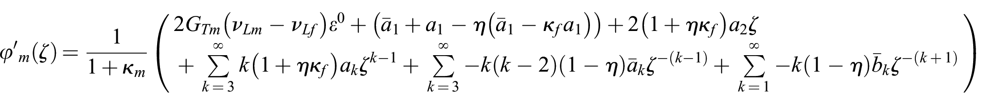
Substituting the expressions of A_k, B_k, C_k, D_k, F_k and H_k as obtained in equation (16) into series (9), those potentials for the matrix can be expressed in terms of a_k, b_k, and c_k as follows:

$$\begin{array}{c}\multicolumn{1}{c}{{\phi }_m=\frac{2G_{\mathrm{Tm}}({\nu }_{\mathrm{Lm}}-{\nu }_{\mathrm{Lf}})}{1+{\kappa }_m}{\epsilon }^0\zeta +\frac{1}{1+{\kappa }_m}({\overline{a}}_1+a_1-\eta ({\overline{a}}_1-{\kappa }_f{a}_1))\zeta +\frac{1+\eta {\kappa }_f}{1+{\kappa }_m}{a}_2{\zeta }^2+\frac{2(1-\eta )}{1+{\kappa }_m}{\overline{a}}_2}\\ \multicolumn{1}{c}{+\frac{1+\eta {\kappa }_f}{1+{\kappa }_m}\sum _{k=3}^{\infty }{a}_k{\zeta }^k+\frac{1-\eta }{1+{\kappa }_m}\sum _{k=3}^{\infty }k{\overline{a}}_k{\zeta }^{-(k-2)}+\frac{1-\eta }{1+{\kappa }_m}\sum _{k=1}^{\infty }{\overline{b}}_k{\zeta }^{-k}}\end{array}$$

$$\begin{array}{c}\multicolumn{1}{c}{{\psi }_m=-\frac{4G_{\mathrm{Tm}}({\nu }_{\mathrm{Lm}}-{\nu }_{\mathrm{Lf}})}{1+{\kappa }_m}{\zeta }^{-1}{\epsilon }^0+\frac{1}{1+{\kappa }_m}({\kappa }_m-1+\eta -\eta {\kappa }_f){\zeta }^{-1}({\overline{a}}_1+a_1)+\frac{2}{1+{\kappa }_m}({\kappa }_m+\eta -1-\eta {\kappa }_f)a_2}\\ +\frac{1}{1+{\kappa }_m}\sum _{k=1}^{\infty }{\zeta }^k((k+2)({\kappa }_m+\eta -1-\eta {\kappa }_f){\overline{a}}_{k+2}+({\kappa }_m+\eta ){\overline{b}}_k)\hfill \\ +\frac{1}{1+{\kappa }_m}\sum _{k=2}^{\infty }{\zeta }^{-k}({\kappa }_m-\eta {\kappa }_f+k(k-2)(1-\eta )){\overline{a}}_k+(k-2)(1-\eta ){\overline{b}}_{k-2}\hfill \end{array}$$

$${\omega }_m=\frac{1}{2}\sum _{k=1}^{\infty }((\lambda +1)c_k{\zeta }^k+(\lambda -1){\overline{c}}_k{\zeta }^{-k}).$$

(17)

In general, between the two phases of different materials, the continuity conditions in displacement and traction will be satisfied as long as series (7) and (9) are truncated in a consistent manner. This can be easily demonstrated if one substitutes equations (7) and (17) into equation (13).

2.4. Relative displacement boundary condition and periodic traction boundary conditions

After satisfying the continuity conditions between the fibre and matrix, coefficients a_k, b_k, and c_k become the only set of unknowns to be determined. The conditions available are the boundary conditions for the unit cell. According to the study by Li and Sitnikova [5,6], they are the relative displacement boundary conditions and the periodic traction boundary conditions. Because the traction boundary conditions involve traction on different parts of the boundary in the same equation, the expression of traction as given in equation (11) is no longer convenient to apply. The periodic traction boundary conditions can be given as [6]:

$$\left[\begin{array}{ccc}{\sigma }_{x\mathrm{\Delta }}\hfill & {\tau }_{\mathrm{xy}\mathrm{\Delta }}\hfill & {\tau }_{\mathrm{xz}\mathrm{\Delta }}\hfill \\ \multicolumn{1}{c}{{\tau }_{\mathrm{xy}\mathrm{\Delta }}}& {\sigma }_{y\mathrm{\Delta }}\hfill & {\tau }_{\mathrm{yz}\mathrm{\Delta }}\hfill \\ \multicolumn{1}{c}{{\tau }_{\mathrm{xz}\mathrm{\Delta }}}& {\tau }_{\mathrm{yz}\mathrm{\Delta }}\hfill & {\sigma }_{z\mathrm{\Delta }}\hfill \end{array}\right]\left\{\begin{array}{c}\cos \beta \hfill \\ \multicolumn{1}{c}{\sin \beta }\\ \multicolumn{1}{c}{0}\end{array}\right\}=\left[\begin{array}{ccc}{\sigma }_x\hfill & {\tau }_{\mathrm{xy}}\hfill & {\tau }_{\mathrm{xz}}\hfill \\ \multicolumn{1}{c}{{\tau }_{\mathrm{xy}}}& {\sigma }_y\hfill & {\tau }_{\mathrm{yz}}\hfill \\ \multicolumn{1}{c}{{\tau }_{\mathrm{xz}}}& {\tau }_{\mathrm{yz}}\hfill & {\sigma }_z\hfill \end{array}\right]\left\{\begin{array}{c}\cos \beta \hfill \\ \multicolumn{1}{c}{\sin \beta }\\ \multicolumn{1}{c}{0}\end{array}\right\}.$$

(18a)

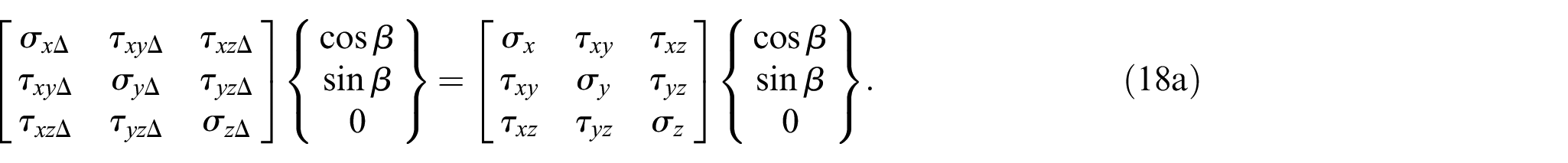
In a GPE problem, the z component of the outward normal to the boundary always vanishes. The outward normal at paired points on the opposite side of the unit cell is the same but opposite in direction, as reflected in equation (18a). Stresses σ_x, σ_y, σ_z, τ_yz, τ_xz and τ_xy, and σ_xΔ, σ_yΔ, σ_zΔ, τ_yzΔ, τ_xzΔ and τ_xyΔ are at paired points, (x, y) and (x_Δ, y_Δ), on the boundary.

The relative displacement boundary conditions for the unit cell are [5,6]:

$$\left\{\begin{array}{c}{u}_{\mathrm{\Delta }}\hfill \\ \multicolumn{1}{c}{v_{\mathrm{\Delta }}}\\ \multicolumn{1}{c}{w_{\mathrm{\Delta }}}\end{array}\right\}-\left\{\begin{array}{c}u\hfill \\ \multicolumn{1}{c}{v}\\ \multicolumn{1}{c}{w}\end{array}\right\}=\left[\begin{array}{ccc}{\epsilon }_x^0\hfill & 0\hfill & 0\hfill \\ \multicolumn{1}{c}{{\gamma }_{\mathrm{xy}}^0}& {\epsilon }_y^0\hfill & 0\hfill \\ \multicolumn{1}{c}{{\gamma }_{\mathrm{xz}}^0}& {\gamma }_{\mathrm{yz}}^0\hfill & {\epsilon }^0\hfill \end{array}\right]\left\{\begin{array}{c}{\mathrm{\Delta }}_x\hfill \\ \multicolumn{1}{c}{{\mathrm{\Delta }}_y}\\ \multicolumn{1}{c}{{\mathrm{\Delta }}_z}\end{array}\right\}=\left[\begin{array}{ccc}{\epsilon }_x^0\hfill & 0\hfill & 0\hfill \\ \multicolumn{1}{c}{{\gamma }_{\mathrm{xy}}^0}& {\epsilon }_y^0\hfill & 0\hfill \\ \multicolumn{1}{c}{{\gamma }_{\mathrm{xz}}^0}& {\gamma }_{\mathrm{yz}}^0\hfill & {\epsilon }^0\hfill \end{array}\right]\left\{\begin{array}{c}\cos \beta \hfill \\ \multicolumn{1}{c}{\sin \beta }\\ \multicolumn{1}{c}{0}\end{array}\right\}\mathrm{\Delta }=\left[\begin{array}{cc}{\epsilon }_x^0\hfill & 0\hfill \\ \multicolumn{1}{c}{{\gamma }_{\mathrm{xy}}^0}& {\epsilon }_y^0\hfill \\ \multicolumn{1}{c}{{\gamma }_{\mathrm{xz}}^0}& {\gamma }_{\mathrm{yz}}^0\hfill \end{array}\right]\left\{\begin{array}{c}\cos \beta \hfill \\ \multicolumn{1}{c}{\sin \beta }\end{array}\right\}\mathrm{\Delta }$$

(18b)

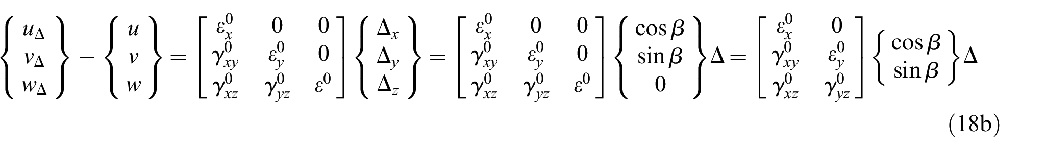
where u, v and w, and u_Δ, v_Δ and w_Δ are the displacements at the paired points, Δ is the distance between the paired points, that is the amount of translation involved in the formulation of the unit cell, with Δ _x , Δ _y and Δ _z as its components, and ${\epsilon }_x^0$ , ${\epsilon }_y^0$ , ${\epsilon }^0$ , ${\gamma }_{\mathrm{yz}}^0$ ${\gamma }_{\mathrm{xz}}^0$ and ${\gamma }_{\mathrm{xy}}^0$ are the average strains in the unit cell. Since the two paired points are always on the same cross-section of the material, they share the common z-coordinate and hence Δ _z  = 0. As a result, ${\epsilon }^0$ will not appear in the actual relative displacement boundary conditions.

To prescribe the periodic traction boundary conditions, all stress components can be expressed in terms of the complex potentials as follows:

$$\begin{array}{c}{\sigma }_{x\mathrm{\Delta }}=\mathrm{Re}(2{\phi \prime }_m({\zeta }_{\mathrm{\Delta }})-{\overline{\zeta }}_{\mathrm{\Delta }}{\phi \prime \prime }_m({\zeta }_{\mathrm{\Delta }})-{\psi \prime }_m({\zeta }_{\mathrm{\Delta }})){\sigma }_x=\mathrm{Re}(2{\phi \prime }_m(\zeta )-\overline{\zeta }{\phi \prime \prime }_m(\zeta )-{\psi \prime }_m(\zeta ))\hfill \\ {\sigma }_{y\mathrm{\Delta }}=\mathrm{Re}(2{\phi \prime }_m({\zeta }_{\mathrm{\Delta }})+{\overline{\zeta }}_{\mathrm{\Delta }}{\phi \prime \prime }_m({\zeta }_{\mathrm{\Delta }})+{\psi \prime }_m({\zeta }_{\mathrm{\Delta }})){\sigma }_y=\mathrm{Re}(2{\phi \prime }_m(\zeta )+\overline{\zeta }{\phi \prime \prime }_m(\zeta )+{\psi \prime }_m(\zeta ))\hfill \\ {\tau }_{\mathrm{xy}\mathrm{\Delta }}=\mathrm{Im}({\overline{\zeta }}_{\mathrm{\Delta }}{\phi \prime \prime }_m({\zeta }_{\mathrm{\Delta }})+{\psi \prime }_m({\zeta }_{\mathrm{\Delta }})){\tau }_{\mathrm{xy}}=\mathrm{Im}(\overline{\zeta }{\phi \prime \prime }_m(\zeta )+{\psi \prime }_m(\zeta ))\hfill \end{array}$$

$$\begin{array}{c}{\tau }_{\mathrm{xz}\mathrm{\Delta }}=\mathrm{Re}{\omega \prime }_m({\zeta }_{\mathrm{\Delta }}){\tau }_{\mathrm{xz}}=\mathrm{Re}{\omega \prime }_m(\zeta )\hfill \\ {\tau }_{\mathrm{yz}\mathrm{\Delta }}=-\mathrm{Im}{\omega \prime }_m({\zeta }_{\mathrm{\Delta }}){\tau }_{\mathrm{yz}}=-\mathrm{Im}{\omega \prime }_m(\zeta )\hfill \end{array}$$

(19)

where all complex potentials involved are those associated with the matrix as the boundary of the unit cell lies completely in the matrix.

The following relationships have been used repeatedly in the derivation:

$$\begin{array}{c}\zeta =\left|\zeta \right|\rho =\left|\zeta \right|e^{i\theta },\overline{\zeta }=\left|\zeta \right|{\rho }^{-1}=\left|\zeta \right|e^{-i\theta },\hfill \\ {\zeta }^k={\left|\zeta \right|}^k{\rho }^k={\left|\zeta \right|}^k{e}^{\mathrm{ik}\theta },\overline{{\zeta }^k}={\left|\zeta \right|}^k{\rho }^{-k}={\left|\zeta \right|}^k{e}^{-\mathrm{ik}\theta },\hfill \\ {\zeta }^{-k}={\left|\zeta \right|}^{-k}{\rho }^{-k}={\left|\zeta \right|}^{-k}{e}^{-\mathrm{ik}\theta },\mathrm{and}\overline{{\zeta }^{-k}}={\left|\zeta \right|}^{-k}{\rho }^k={\left|\zeta \right|}^{-k}{e}^{\mathrm{ik}\theta }.\hfill \end{array}$$

(20)

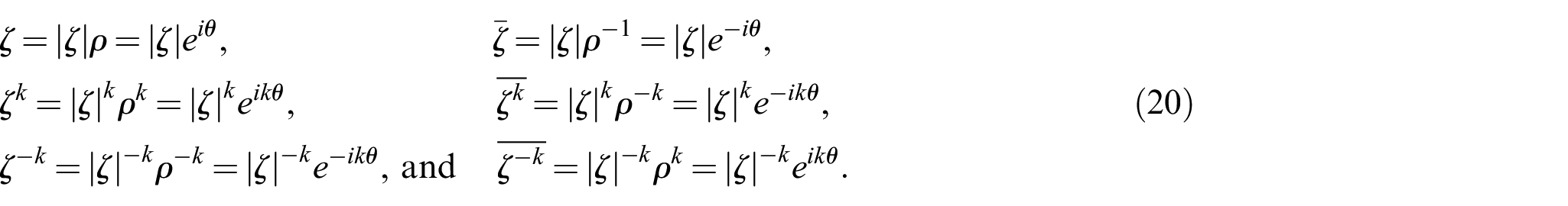
In the present GPE problem, the part within the plane of the cross-section and the part out of this plane are fully decoupled. They can be addressed separately for both clarity and computational efficiency. The part in the cross-section plane will be considered first below. The terms involved can be given in the form of series containing unknown coefficients a_k, b_k, and c_k and their conjugates only as follows:

$$\phi {\prime }_m\left(\zeta \right)=\frac{1}{1+{\kappa }_m}\left(\begin{array}{c}2G_{\mathrm{Tm}}({\nu }_{\mathrm{Lm}}-{\nu }_{\mathrm{Lf}}){\epsilon }^0+({\overline{a}}_1+a_1-\eta ({\overline{a}}_1-{\kappa }_f{a}_1))+2(1+\eta {\kappa }_f)a_2\zeta \hfill \\ \multicolumn{1}{c}{+\sum _{k=3}^{\infty }k(1+\eta {\kappa }_f)a_k{\zeta }^{k-1}+\sum _{k=3}^{\infty }-k(k-2)(1-\eta ){\overline{a}}_k{\zeta }^{-(k-1)}+\sum _{k=1}^{\infty }-k(1-\eta ){\overline{b}}_k{\zeta }^{-(k+1)}}\end{array}\right)$$

$$\overline{\zeta }\phi \prime {\prime }_m\left(\zeta \right)=\frac{1}{1+{\kappa }_m}\left(\begin{array}{c}2(1+\eta {\kappa }_f)a_2\left|\zeta \right|{\rho }^{-1}+\sum _{k=3}^{\infty }k(k-1)(1+\eta {\kappa }_f)a_k{\left|\zeta \right|}^{k-1}{\rho }^{k-3}\hfill \\ \multicolumn{1}{c}{+\sum _{k=3}^{\infty }k(k-1)(k-2)(1-\eta ){\overline{a}}_k{\left|\zeta \right|}^{-(k-1)}{\rho }^{-(k+1)}+\sum _{k=1}^{\infty }k(k+1)(1-\eta ){\overline{b}}_k{\left|\zeta \right|}^{-(k+1)}{\rho }^{-(k+3)}}\end{array}\right)$$

$$\psi {\prime }_m\left(\zeta \right)=\frac{1}{1+{\kappa }_m}\left(\begin{array}{c}4G_{\mathrm{Tm}}({\nu }_{\mathrm{Lm}}-{\nu }_{\mathrm{Lf}}){\zeta }^{-2}{\epsilon }^0-({\kappa }_m-1+\eta -\eta {\kappa }_f){\zeta }^{-2}({\overline{a}}_1+a_1)-2({\kappa }_m-\eta {\kappa }_f){\zeta }^{-3}{\overline{a}}_2\hfill \\ \multicolumn{1}{c}{+\sum _{k=3}^{\infty }k(k-2)({\kappa }_m+\eta -1-\eta {\kappa }_f){\zeta }^{k-3}{a}_k-\sum _{k=3}^{\infty }k({\kappa }_m-\eta {\kappa }_f+k(k-2)(1-\eta )){\zeta }^{-(k+1)}{\overline{a}}_k}\\ \multicolumn{1}{c}{+\sum _{k=1}^{\infty }k({\kappa }_m+\eta ){\zeta }^{k-1}{b}_k-\sum _{k=1}^{\infty }k(k+2)(1-\eta ){\zeta }^{-(k+3)}{\overline{b}}_k}\end{array}\right).$$

(21)

Replacing ζ with ζ_Δ, one obtains $\phi {\prime }_m({\zeta }_{\mathrm{\Delta }})$ , ${\overline{\zeta }}_{\mathrm{\Delta }}\phi \prime {\prime }_m({\zeta }_{\mathrm{\Delta }})$ , and $\psi {\prime }_m({\zeta }_{\mathrm{\Delta }})$ accordingly, where ζ and ζ_Δ are the complex coordinates of the two paired points (x, y) and (x_Δ, y_Δ). Then, the periodic traction boundary conditions can be expressed as:

$$\begin{array}{c}\mathrm{Re}(2{\phi \prime }_m({\zeta }_{\mathrm{\Delta }})-{\overline{\zeta }}_{\mathrm{\Delta }}{\phi \prime \prime }_m({\zeta }_{\mathrm{\Delta }})-{\psi \prime }_m({\zeta }_{\mathrm{\Delta }}))\cos \beta +\mathrm{Im}({\overline{\zeta }}_{\mathrm{\Delta }}{\phi \prime \prime }_m({\zeta }_{\mathrm{\Delta }})+{\psi \prime }_m({\zeta }_{\mathrm{\Delta }}))\sin \beta \hfill \\ =\mathrm{Re}(2{\phi \prime }_m(\zeta )-\overline{\zeta }{\phi \prime \prime }_m(\zeta )-{\psi \prime }_m(\zeta ))\cos \beta +\mathrm{Im}(\overline{\zeta }{\phi \prime \prime }_m(\zeta )+{\psi \prime }_m(\zeta ))\sin \beta \hfill \\ \mathrm{Im}({\overline{\zeta }}_{\mathrm{\Delta }}{\phi \prime \prime }_m({\zeta }_{\mathrm{\Delta }})+{\psi \prime }_m({\zeta }_{\mathrm{\Delta }}))\cos \beta +\mathrm{Re}(2{\phi \prime }_m({\zeta }_{\mathrm{\Delta }})+{\overline{\zeta }}_{\mathrm{\Delta }}{\phi \prime \prime }_m({\zeta }_{\mathrm{\Delta }})+{\psi \prime }_m({\zeta }_{\mathrm{\Delta }}))\sin \beta \hfill \\ =\mathrm{Im}(\overline{\zeta }{\phi \prime \prime }_m(\zeta )+{\psi \prime }_m(\zeta ))\cos \beta +\mathrm{Re}(2{\phi \prime }_m(\zeta )+\overline{\zeta }{\phi \prime \prime }_m(\zeta )+{\psi \prime }_m(\zeta ))\sin \beta .\hfill \end{array}$$

(22a)

Since they are paired, with the origin of the coordinate system being placed at the centre of the unit cell, the polar radii of these two points are always the same, that is,

$$\left|{\zeta }_{\mathrm{\Delta }}\right|=\left|\zeta \right|.$$

(23)

Substituting equation (21) and their counterparts associated with ζ_Δ into equation (22a), the periodic traction boundary conditions in the cross-section plane become:

$$\begin{array}{c}(2\mathrm{Re}{Q}_1-\mathrm{Re}{Q}_2)\cos \beta +\mathrm{Im}{Q}_2\sin \beta =-\mathrm{Re}R\cos \beta +\mathrm{Im}R\sin \beta \hfill \\ (2\mathrm{Re}{Q}_1+\mathrm{Re}{Q}_2)\sin \beta +\mathrm{Im}{Q}_2\cos \beta =\mathrm{Re}R\sin \beta +\mathrm{Im}R\cos \beta \hfill \end{array}$$

(22b)

where

$$Q_1=\left(\begin{array}{c}2(1+\eta {\kappa }_f)\left|\zeta \right|({\rho }_{\mathrm{\Delta }}-\rho )a_2\hfill \\ \multicolumn{1}{c}{+\sum _{k=3}^{\infty }k(1+\eta {\kappa }_f){\left|\zeta \right|}^{k-1}({{\rho }_{\mathrm{\Delta }}}^{k-1}-{\rho }^{k-1})a_k}\\ \multicolumn{1}{c}{-\sum _{k=3}^{\infty }k(k-2)(1-\eta ){\left|\zeta \right|}^{-(k-1)}({{\rho }_{\mathrm{\Delta }}}^{-(k-1)}-{\rho }^{-(k-1)}){\overline{a}}_k}\\ \multicolumn{1}{c}{-\sum _{k=1}^{\infty }k(1-\eta ){\left|\zeta \right|}^{-(k+1)}({{\rho }_{\mathrm{\Delta }}}^{-(k+1)}-{\rho }^{-(k+1)}){\overline{b}}_k}\end{array}\right)$$

(24a)

$$Q_2=\left(\begin{array}{c}-({\kappa }_m-1+\eta -\eta {\kappa }_f){\left|\zeta \right|}^{-2}({{\rho }_{\mathrm{\Delta }}}^{-2}-{\rho }^{-2})a_1\hfill \\ \multicolumn{1}{c}{-({\kappa }_m-1+\eta -\eta {\kappa }_f){\left|\zeta \right|}^{-2}({{\rho }_{\mathrm{\Delta }}}^{-2}-{\rho }^{-2}){\overline{a}}_1}\\ \multicolumn{1}{c}{+2(1+\eta {\kappa }_f)\left|\zeta \right|({{\rho }_{\mathrm{\Delta }}}^{-1}-{\rho }^{-1})a_2}\\ \multicolumn{1}{c}{-2({\kappa }_m-\eta {\kappa }_f){\left|\zeta \right|}^{-3}({{\rho }_{\mathrm{\Delta }}}^{-3}-{\rho }^{-3}){\overline{a}}_2}\\ \multicolumn{1}{c}{+\sum _{k=3}^{\infty }k\left(\begin{array}{c}(k-1)(1+\eta {\kappa }_f){\left|\zeta \right|}^{k-1}\hfill \\ \multicolumn{1}{c}{+(k-2)({\kappa }_m+\eta -1-\eta {\kappa }_f){\left|\zeta \right|}^{k-3}}\end{array}\right)({{\rho }_{\mathrm{\Delta }}}^{k-3}-{\rho }^{k-3})a_k}\\ \multicolumn{1}{c}{+\sum _{k=3}^{\infty }k\left(\begin{array}{c}(k-1)(k-2)(1-\eta ){\left|\zeta \right|}^{-(k-1)}\hfill \\ \multicolumn{1}{c}{-({\kappa }_m-\eta {\kappa }_f+k(k-2)(1-\eta )){\left|\zeta \right|}^{-(k+1)}}\end{array}\right)({{\rho }_{\mathrm{\Delta }}}^{-(k+1)}-{\rho }^{-(k+1)}){\overline{a}}_k}\\ \multicolumn{1}{c}{+\sum _{k=1}^{\infty }k({\kappa }_m+\eta ){\left|\zeta \right|}^{k-1}({{\rho }_{\mathrm{\Delta }}}^{k-1}-{\rho }^{k-1})b_k}\\ \multicolumn{1}{c}{+\sum _{k=1}^{\infty }k(1-\eta )((k+1){\left|\zeta \right|}^{-(k+1)}-(k+2){\left|\zeta \right|}^{-(k+3)})({{\rho }_{\mathrm{\Delta }}}^{-(k+3)}-{\rho }^{-(k+3)}){\overline{b}}_k}\end{array}\right)$$

(24b)

$$R=-4G_{\mathrm{Tm}}({\nu }_{\mathrm{Lm}}-{\nu }_{\mathrm{Lf}}){\left|\zeta \right|}^{-2}({{\rho }_{\mathrm{\Delta }}}^{-2}-{\rho }^{-2}){\epsilon }^0.$$

(24c)

Equation (23) is the periodic traction boundary conditions for the unit cell. They are simultaneous equations for the unknowns a_k, b_k, and c_k and their conjugates, with expressions Q₁, Q₂ and R involved given in equation (24), respectively.

Now, attention can be moved to the relative displacement boundary conditions. According to equation (6a), displacements in the cross-section plane can be expressed in terms of the following terms:

$${\phi }_m\left(\zeta \right)=\frac{1}{1+{\kappa }_m}\left(\begin{array}{c}2G_{\mathrm{Tm}}({\nu }_{\mathrm{Lm}}-{\nu }_{\mathrm{Lf}}){\epsilon }^0\left|\zeta \right|\rho +(a_1+{\overline{a}}_1+\eta {\kappa }_f{a}_1-\eta {\overline{a}}_1)\left|\zeta \right|\rho \hfill \\ \multicolumn{1}{c}{+(1+\eta {\kappa }_f)a_2{\left|\zeta \right|}^2{\rho }^2+2(1-\eta ){\overline{a}}_2}\\ \multicolumn{1}{c}{+\sum _{k=3}^{\infty }(1+\eta {\kappa }_f)a_k{\left|\zeta \right|}^k{\rho }^k+\sum _{k=3}^{\infty }k(1-\eta ){\overline{a}}_k{\left|\zeta \right|}^{-(k-2)}{\rho }^{-(k-2)}}\\ \multicolumn{1}{c}{+\sum _{k=1}^{\infty }(1-\eta ){\overline{b}}_k{\left|\zeta \right|}^{-k}{\rho }^{-k}}\end{array}\right)$$

(25a)

$$\zeta \overline{\phi }{\prime }_m\left(\zeta \right)=\frac{1}{1+{\kappa }_m}\left(\begin{array}{c}2G_{\mathrm{Tm}}({\nu }_{\mathrm{Lm}}-{\nu }_{\mathrm{Lf}})\left|\zeta \right|\rho {\epsilon }^0+(a_1+{\overline{a}}_1+\eta {\kappa }_f{\overline{a}}_1-\eta a_1)\left|\zeta \right|\rho \hfill \\ \multicolumn{1}{c}{+2(1+\eta {\kappa }_f){\left|\zeta \right|}^2{\overline{a}}_2}\\ \multicolumn{1}{c}{+\sum _{k=3}^{\infty }k(1+\eta {\kappa }_f){\left|\zeta \right|}^k{\rho }^{-(k-2)}{\overline{a}}_k-\sum _{k=3}^{\infty }k(k-2)(1-\eta ){\left|\zeta \right|}^{-(k-2)}{\rho }^k{a}_k}\\ \multicolumn{1}{c}{-\sum _{k=1}^{\infty }k(1-\eta ){\left|\zeta \right|}^{-k}{\rho }^{k+2}{b}_k}\end{array}\right)$$

(25b)

$${\overline{\psi }}_m\left(\zeta \right)=\frac{1}{1+{\kappa }_m}\left(\begin{array}{c}-4G_{\mathrm{Tm}}({\nu }_{\mathrm{Lm}}-{\nu }_{\mathrm{Lf}}){\left|\zeta \right|}^{-1}\rho {\epsilon }^0+({\kappa }_m-1+\eta -\eta {\kappa }_f){\left|\zeta \right|}^{-1}\rho ({\overline{a}}_1+a_1)\hfill \\ \multicolumn{1}{c}{+2({\kappa }_m+\eta -1-\eta {\kappa }_f){\overline{a}}_2+({\kappa }_m-\eta {\kappa }_f){\left|\zeta \right|}^{-2}{\rho }^2{a}_2}\\ \multicolumn{1}{c}{+\sum _{k=3}^{\infty }k({\kappa }_m+\eta -1-\eta {\kappa }_f){\left|\zeta \right|}^{k-2}{\rho }^{-(k-2)}{\overline{a}}_k}\\ \multicolumn{1}{c}{+\sum _{k=3}^{\infty }({\kappa }_m-\eta {\kappa }_f+k(k-2)(1-\eta )){\left|\zeta \right|}^{-k}{\rho }^k{a}_k}\\ \multicolumn{1}{c}{+\sum _{k=1}^{\infty }({\kappa }_m+\eta ){\left|\zeta \right|}^k{\rho }^{-k}{\overline{b}}_k+\sum _{k=1}^{\infty }k(1-\eta ){\left|\zeta \right|}^{-(k+2)}{\rho }^{k+2}{b}_k}\end{array}\right).$$

(25c)

Replacing ζ with ζ_Δ, one obtains ${\phi }_m({\zeta }_{\mathrm{\Delta }})$ , ${\zeta }_{\mathrm{\Delta }}\overline{\phi }{\prime }_m({\zeta }_{\mathrm{\Delta }})$ , and ${\overline{\psi }}_m({\zeta }_{\mathrm{\Delta }})$ accordingly. Then, the relative displacement boundary conditions in the cross-section plane can be obtained as:

$$\begin{array}{c}{\kappa }_m{\phi }_m\left({\zeta }_{\mathrm{\Delta }}\right)-{\zeta }_{\mathrm{\Delta }}\overline{{\phi \prime }_m\left({\zeta }_{\mathrm{\Delta }}\right)}-\overline{{\psi }_m\left({\zeta }_{\mathrm{\Delta }}\right)}-({\kappa }_m{\phi }_m\left(\zeta \right)-\zeta \overline{{\phi \prime }_m\left(\zeta \right)}-\overline{{\psi }_m\left(\zeta \right)})\hfill \\ =2G_{\mathrm{Tm}}{\nu }_{\mathrm{Lm}}{\epsilon }^0({\zeta }_{\mathrm{\Delta }}-\zeta )+2G_{\mathrm{Tm}}({\epsilon }_x^0\cos \beta +i({\gamma }_{\mathrm{xy}}^0\cos \beta +{\epsilon }_y^0\sin \beta ))\mathrm{\Delta }.\hfill \end{array}$$

(26a)

Substituting equation (25) and their counterparts associated with ζ_Δ into equation (26a), the relative displacement boundary conditions in the cross-section plane can be given explicitly as,

$$\begin{array}{c}(({\kappa }_m-1+\eta {\kappa }_m{\kappa }_f+\eta )\left|\zeta \right|-({\kappa }_m-1+\eta -\eta {\kappa }_f){\left|\zeta \right|}^{-1})({\rho }_{\mathrm{\Delta }}-\rho )a_1\hfill \\ (({\kappa }_m-1-\eta {\kappa }_m-\eta {\kappa }_f)\left|\zeta \right|-({\kappa }_m-1+\eta -\eta {\kappa }_f){\left|\zeta \right|}^{-1})({\rho }_{\mathrm{\Delta }}-\rho ){\overline{a}}_1\hfill \\ +({\kappa }_m(1+\eta {\kappa }_f){\left|\zeta \right|}^2-({\kappa }_m-\eta {\kappa }_f){\left|\zeta \right|}^{-2})({\rho }_{\mathrm{\Delta }}^2-{\rho }^2)a_2\hfill \\ +\sum _{k=3}^{\infty }({\kappa }_m(1+\eta {\kappa }_f){\left|\zeta \right|}^k-({\kappa }_m-\eta {\kappa }_f){\left|\zeta \right|}^{-k}+k(k-2)(1-\eta )({\left|\zeta \right|}^{-(k-2)}-{\left|\zeta \right|}^{-k}))({\rho }_{\mathrm{\Delta }}^k-{\rho }^k)a_k\hfill \\ +\sum _{k=3}^{\infty }k({\kappa }_m(1-\eta ){\left|\zeta \right|}^{-(k-2)}-(1+\eta {\kappa }_f){\left|\zeta \right|}^k-({\kappa }_m+\eta -1-\eta {\kappa }_f){\left|{\zeta }_{\mathrm{\Delta }}\right|}^{k-2})({\rho }_{\mathrm{\Delta }}^{-(k-2)}-{\rho }^{-(k-2)}){\overline{a}}_k\hfill \end{array}$$

$$\begin{array}{c}+\sum _{k=1}^{\infty }k(1-\eta )({\left|\zeta \right|}^{-k}-{\left|\zeta \right|}^{-(k+2)})({\rho }_{\mathrm{\Delta }}^{k+2}-{\rho }^{k+2})b_k\hfill \\ +\sum _{k=1}^{\infty }({\kappa }_m(1-\eta ){\left|\zeta \right|}^{-k}-({\kappa }_m+\eta ){\left|\zeta \right|}^k)({\rho }_{\mathrm{\Delta }}^{-k}-{\rho }^{-k}){\overline{b}}_k\hfill \end{array}$$

$$\begin{array}{c}=2G_{\mathrm{Tm}}(1+{\kappa }_m)({\epsilon }_x^0\cos \beta +i({\gamma }_{\mathrm{xy}}^0\cos \beta +{\epsilon }_y^0\sin \beta ))\mathrm{\Delta }\hfill \\ +2G_{\mathrm{Tm}}({\nu }_{\mathrm{Lm}}(1+{\kappa }_m)\left|\zeta \right|-({\nu }_{\mathrm{Lm}}-{\nu }_{\mathrm{Lf}})(({\kappa }_m-1)\left|\zeta \right|+2{\left|\zeta \right|}^{-1}))({\rho }_{\mathrm{\Delta }}-\rho ){\epsilon }^0.\hfill \end{array}$$

(26b)

The boundary conditions obtained above in equations (23) and (26b) are all defined between paired points on opposite sides of the boundary of the unit cell. For a square unit cell, there are two pairs of opposite side and for hexagonal one, there are three pairs.

2.5. The point matching method

In theory, if all series involved kept infinite number of terms and the above boundary conditions were satisfied at every pair of points on the boundary of the unit cell, exact solution could be obtained. In practice, the solution for a_k and b_k involves inverting the coefficient matrix. Having infinite terms in the series would mean that the coefficient matrix has infinite number of rows and columns. The inverse of such an infinite matrix is beyond possibility, in general. The series will have to be truncated somewhere and the inverse can only be found numerically practically. As a result, the boundary conditions for the unit cell can only be satisfied approximately one way or another.

Accordingly, another approximation has to be made and the number of paired points can only be finite as it is impossible to prescribe those boundary conditions continuously along the boundary and they have to be imposed at finite number of discrete points. Apparently, the more pairs involved, the better the approximation. However, more pairs of points involved also imply that there will be more equations. Eventually, they can quickly run to a number greater than the number of unknowns, leading to an overdetermined system of equations for which a solution strictly satisfying all equations would not exist in general. It is usually not an option to keep the number of equations exactly the same as the number of unknowns. Some of the equations may not be fully independent, in particular, those obtained at the ends of each pair of opposite sides. An ill-conditioned set of simultaneous equations can easily arise as a result. It is therefore beneficial to increase the number of paired points artificially and then seek a reasonable solution to the overdetermined system of equations somehow, as will be explored later.

Assuming that all series are truncated at Nth order, for each pair of points on the boundary, two equations of complex coefficients can be obtained according to equations (23) and (26b). They are for 2N pairs of conjugating complex unknowns:

$${[a_1{\overline{a}}_1{b}_1{\overline{b}}_1{a}_2{\overline{a}}_2{b}_2{\overline{b}}_2\cdots a_N{\overline{a}}_N{b}_N{\overline{b}}_N]}^T.$$

(27)

Unfortunately, there have not been many established complex solvers for simultaneous equations. It is more convenient to convert these complex equations into real ones instead. The real part Re and imaginary part Im are fairly standard operations in most modern computing languages that can be resorted to directly. Any complex number and its conjugate can be easily related to its real and imaginary parts. This can be illustrated as follows, taking $a_k$ and ${\overline{a}}_k$ as an example:

$$\left\{\begin{array}{c}{a}_k\hfill \\ \multicolumn{1}{c}{{\overline{a}}_k}\end{array}\right\}=\left[\begin{array}{cc}1\hfill & i\hfill \\ \multicolumn{1}{c}{1}& -i\hfill \end{array}\right]\left\{\begin{array}{c}\mathrm{Re}{a}_k\hfill \\ \multicolumn{1}{c}{\mathrm{Im}{a}_k}\end{array}\right\}.$$

(28)

Thus, four real equations can be obtained from equations (23) and (26b), the unknowns in real form can be given as:

$$\left[X\right]=\{{[\mathrm{Re}{a}_1\mathrm{Im}{a}_1\mathrm{Re}{b}_1\mathrm{Im}{b}_1\mathrm{Re}{a}_2\mathrm{Im}{a}_2\mathrm{Re}{b}_2\mathrm{Im}{b}_2\cdots \mathrm{Re}{a}_N\mathrm{Im}{a}_N\mathrm{Re}{b}_N\mathrm{Im}{b}_N]}^T$$

(29)

There should be four columns in [X], corresponding to four loading cases involved in the GPE problem in the cross-section plane, three due to prescribed average direct strains and one due to average shear strain. These average strains as the loads applied to the unit cell can be presented in arbitrary combinations in theory without compromising the solvability of the problem. However, for the purpose of numerical material characterisation, uniaxial direct strain states and a pure shear strain state are the most relevant ones to the subsequent extraction of effective material properties. Such four loading cases can be analysed in one go efficiently. There will be four solutions accordingly and they are associated with each of the four loading cases to provide the coefficients in series (7) and (9) for each of the loading cases. The complex potentials given by these series are the solution to the elastic problem.

When the properties of the fibre and the matrix are of different material properties, only approximate solutions can be obtained in general as truncated series involving 4N unknowns. The solution obtained is therefore considered as semi-analytical.

As has been noted before, from each pair of points on boundary, only four real equations can be obtained from equations (23) and (26b). They are insufficient to solve for 4N unknown, in general. Boundary conditions (23) and (26b) must be applied to sufficient number of pairs on the boundary to reach sufficient number of equations.

A relatively established numerical method is the so-called point matching method [18] as a type of weighted residual method in general. To implement, a series of M points are selected on each side along the boundary. It is important that these points are spread along the boundary, evenly if it is more convenient. Denoting n as the number of pairs of sides in the unit cell, 4nM equations can be obtained from equations (23) and (26b) for the 4N unknowns. As explained earlier, sufficient number of pairs of points must be selected, that is nM > N. In general, nM needs to be sufficiently greater than N. Thus, the number of equations 4M is sufficiently greater the number of unknowns 4N to deliver an overdetermined system of 4nM equations for 4N unknowns as follows:

$$\left[K\right]\left[X\right]=\left[B\right]$$

(30)

where the number of rows in coefficient matrix [K] is sufficiently greater than the number of columns, and hence the system is overdetermined. The so-called solution is in fact a compromise which leads to the lowest degree of contradiction. In terms of the boundary conditions of the unit cell, it represents a solution which agrees with the prescribed boundary conditions as much as possible. As has been pointed out already, the continuity conditions between the fibre and matrix across the interface are always satisfied.

A solver for overdetermined system of equations is available in MATLAB [13] based on the least square method, lscov, which can be adopted.

All equations in equation (30) are obtained at discrete pairs of points. There can be as many points as one wishes in principle. In much the same way, the number of terms in the series for the complex potentials can be kept as many as one wishes. Through the synergy of sufficient number of points and sufficient number of terms in the complex potentials, the error in the boundary conditions of the unit cell can be kept as low as one wishes.

There are four average strains involved in equation (26b) corresponding to four loading conditions. When each of them is assigned a unit value under its corresponding loading case, four solutions are obtained, from which the stress distributions can be obtained, and the average stresses, as will be addressed later.

2.6. Solution for the part of problem out of the cross-section plane

The boundary conditions for the part of the problem out of the cross-section plane can be elaborated in a similar way. These equations are all real in nature, although they are expressed in terms of complex potentials. This is because each complex potential appears along with its conjugate and hence the imaginary parts have been cancelled. The out of the cross-section plane periodic traction condition is,

$$\mathrm{Re}\omega {\prime }_m\left({\zeta }_{\mathrm{\Delta }}\right)\cos \beta -\mathrm{Im}\omega {\prime }_m\left({\zeta }_{\mathrm{\Delta }}\right)\sin \beta =\mathrm{Re}\omega {\prime }_m\left(\zeta \right)\cos \beta -\mathrm{Im}\omega {\prime }_m\left(\zeta \right)\sin \beta$$

(31a)

where

$$\omega {\prime }_m\left(\zeta \right)=\frac{1}{2}\sum _{k=1}^{\infty }k((\lambda +1)c_k{\zeta }^{k-1}-(\lambda -1){\overline{c}}_k{\zeta }^{-(k+1)}).$$

(32)

Replacing ζ with ζ_Δ, one obtains $\omega {\prime }_m({\zeta }_{\mathrm{\Delta }})$ . Expressed in terms of the real and imaginary parts of the coefficients of series in equation (7), the corresponding linear equation becomes,

$$\begin{array}{c}\left(\mathrm{Re}\sum _{k=1}^{\infty }k((\lambda +1)c_k({{\zeta }_{\mathrm{\Delta }}}^{k-1}-{\zeta }^{k-1})-(\lambda -1){\overline{c}}_k({{\zeta }_{\mathrm{\Delta }}}^{-(k+1)}-{\zeta }^{-(k+1)}))\right)\cos \beta \hfill \\ -\left(\mathrm{Im}\sum _{k=1}^{\infty }k((\lambda +1)c_k({{\zeta }_{\mathrm{\Delta }}}^{k-1}-{\zeta }^{k-1})-(\lambda -1){\overline{c}}_k({{\zeta }_{\mathrm{\Delta }}}^{-(k+1)}-{\zeta }^{-(k+1)}))\right)\sin \beta =0.\hfill \end{array}$$

(31b)

The relative displacement boundary condition is:

$$\mathrm{Re}{\omega }_m\left({\zeta }_{\mathrm{\Delta }}\right)-\mathrm{Re}{\omega }_m\left(\zeta \right)=G_{\mathrm{Lm}}({\gamma }_{\mathrm{xz}}^0\cos \beta +{\gamma }_{\mathrm{yz}}^0\sin \beta )\mathrm{\Delta }$$

(33a)

where

$${\omega }_m\left(\zeta \right)=\frac{1}{2}\sum _{k=1}^{\infty }((\lambda +1){\left|\zeta \right|}^k{\rho }^k{c}_k+(\lambda -1){\left|\zeta \right|}^{-k}{\rho }^{-k}{\overline{c}}_k).$$

(34)

Replacing ζ with ζ_Δ, ${\omega }_m({\zeta }_{\mathrm{\Delta }})$ is obtained. It can be expressed explicitly in terms of the real and imaginary parts of the coefficients of series in equation (7) as:

$$\mathrm{Re}\sum _{k=1}^N((\lambda +1)({{\zeta }_{\mathrm{\Delta }}}^k-{\zeta }^k)c_k+(\lambda -1)({{\zeta }_{\mathrm{\Delta }}}^{-k}-{\zeta }^{-k}){\overline{c}}_k)=2G_{\mathrm{Lm}}({\gamma }_{\mathrm{xz}}^0\cos \beta +{\gamma }_{\mathrm{yz}}^0\sin \beta )\mathrm{\Delta }.$$

(33b)

For each pair of points on opposite sides of the boundary of the unit cell, one has equations (32) and (34) which are similar to equations (23) and (26b), and they can be treated in a way similar to that in the previous subsection, leading to equations similar to equation (30), except that it is simpler as there are only 2ηM rows and 2N columns in the coefficient matrix [K]. On its right-hand side, there are only two average strains defining two loading cases. As a result, there are two columns in matrix [B], leading to two sets of solutions. As for the paired points on the boundary, although they do not have to be the same as for the case in the plane of the cross-section, it is convenient to keep them the same. This makes the subsequent coding as simple as possible and computational efficiency as high as possible.

The 2N unknowns can be listed as follows:

$$\left[X\right]={[\mathrm{Re}{c}_1\mathrm{Im}{c}_1\mathrm{Re}{c}_2\mathrm{Im}{c}_2\cdots \mathrm{Re}{c}_N\mathrm{Im}{c}_N]}^T$$

(35)

where there are two columns in [X], corresponding to the two loading cases of the unit cell for the pure shear strain states out of the plane of the cross-section.

After solving the problem out of cross-section plane, the complex potentials for the fibre part of the unit cell φ_f, ψ_f and ω_f can all be obtained approximately from equation (7). Those for the matrix part of the unit cell, φ_m, ψ_m and ω_m can be obtained accordingly from equation (9), given equation (16). They are all truncated at the Nth order. Thus, stresses and displacements can be obtained from equations (2), (5a), (5b), (6a), and (6b). There are six sets of them, corresponding to six loading cases.

2.7. Average stresses

The average stresses can be obtained as follows according to their definition. Using the formulae derived in the study by Li and Sitnikova [6], they can be expressed as:

$${\sigma }_x^0=\frac{1}{A}\int \underset{A}{\int }{\sigma }_x\mathrm{dA}=\frac{1}{A}{\oint }_{\partial A}\mathrm{xXds}=\frac{1}{A}{\oint }_{\partial A}x({\sigma }_x\cos \beta +{\tau }_{\mathrm{xy}}\sin \beta )\mathrm{ds}$$

$${\sigma }_y^0=\frac{1}{A}\int \underset{A}{\int }{\sigma }_y\mathrm{dA}=\frac{1}{A}{\oint }_{\partial A}\mathrm{yYds}=\frac{1}{A}{\oint }_{\partial A}y({\tau }_{\mathrm{xy}}\cos \beta +{\sigma }_y\sin \beta )\mathrm{ds}$$

$$\begin{array}{c}{\tau }_{\mathrm{xy}}^0=\frac{1}{A}\int \underset{A}{\int }{\tau }_{\mathrm{xy}}\mathrm{dA}=\frac{1}{A}{\oint }_{\partial A}\mathrm{xXds}=\frac{1}{A}{\oint }_{\partial A}x({\tau }_{\mathrm{xy}}\cos \beta +{\sigma }_y\sin \beta )\mathrm{ds}\hfill \\ =\frac{1}{A}{\oint }_{\partial A}\mathrm{yYds}=\frac{1}{A}{\oint }_{\partial A}y({\sigma }_x\cos \beta +{\tau }_{\mathrm{xy}}\sin \beta )\mathrm{ds}\hfill \end{array}$$

(36a)

$${\tau }_{\mathrm{yz}}^0=\frac{1}{A}\int \underset{A}{\int }{\tau }_{\mathrm{yz}}\mathrm{dA}=\frac{1}{A}{\oint }_{\partial A}\mathrm{yZds}=\frac{1}{A}{\oint }_{\partial A}y({\tau }_{\mathrm{xz}}\cos \beta +{\tau }_{\mathrm{yz}}\sin \beta )\mathrm{ds}$$

$${\tau }_{\mathrm{xz}}^0=\frac{1}{A}\int \underset{A}{\int }{\tau }_{\mathrm{xz}}\mathrm{dA}=\frac{1}{A}{\oint }_{\partial A}\mathrm{xZds}=\frac{1}{A}{\oint }_{\partial A}x({\tau }_{\mathrm{xz}}\cos \beta +{\tau }_{\mathrm{yz}}\sin \beta )\mathrm{ds}$$

where X, Y, and Z are traction on the unit circle as expressed in equation (10),

$$A=\{\begin{array}{cc}{\mathrm{\Delta }}^2\hfill & \mathrm{squre}\mathrm{unit}\mathrm{cell}\hfill \\ \multicolumn{1}{c}{\frac{\sqrt{3}{\mathrm{\Delta }}^2}{2}}& \mathrm{hexagonal}\mathrm{unit}\mathrm{cell}\hfill \end{array}$$

(37)

and symbol A represents the cross-section area of the unit cell and the domain for this area without confusion. As integrals over A, these average stresses include both the fibre and the matrix. However, as line integrals, they only involve the boundary of the unit cell ∂A. This can be argued as follows. The stresses in the unit cell are not necessarily continuous across the interface between fibre and matrix. An area integration usually has to be evaluated separately between fibre and matrix before summing both parts together. When the divergence theorem is applied to the fibre and matrix parts separately, one obtains a line integration for each part. The line integration for the fibre part is straightforward. As a doubly connected domain, the matrix part has to be turned into a singly connected domain first by cutting it apart, for example, along the dashed line as indicated in Figure 2. Along the opposite sides of the cut, the directions of the integration paths are opposite and the values of the integrations over these two segments cancel each other. Along the interface between the fibre and matrix, the line integrations on both sides are for different parts of the unit cell. However, the factor of the integrands, for example X, happens to be the components of the traction and the continuity condition requires that they take the same value on both sides of the interface. The other factor x or y outside the brackets is the coordinate on the interface and therefore also shared by both sides. As a result, they end up with the same value of their counterparts from the fibre, but opposite in sense because the directions of their integration paths are opposite to each other. They cancel each other, leaving behind only the line integration along the external boundary of the unit cell ∂A.

Figure 2.

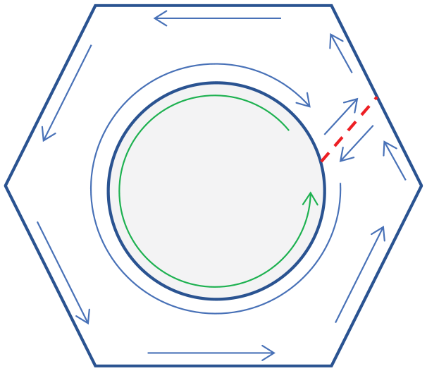
The paths for line integrations.

The boundary of the unit cell involves matrix only, so are the line integrations. They can be easily integrated numerically, for instance, using the trapezium rule. Thus, the evaluation of these integrations reduces to a matter of computing the values of series (9) at the selected points on the boundary of the unit cell. In particular, when these points are equally spaced, for example, by a distance h apart, an integration along the complete boundary becomes h times the sum of the values of the integrand function at all selected points, except the ends of each side of the boundary. According to the trapezium rule, the ends make half of the contribution of an interior point. However, given the closed nature of the boundary, each end appears on two neighbouring sides at their intersection. There will be two halves of the contribution from either side. The integrand is usually not continuous from one side to the other at the corner. However, this does not affect the evaluation of integrations in any way.

The conclusion drawn is applicable to each of the integrations listed in equation (36a). However, its general applicability cannot be taken for granted. In the case of GPE problem, the average stress in the fibre direction is a case the conclusion does not apply. From equation (2), one has,

$$\begin{array}{c}\multicolumn{1}{c}{{\sigma }_z^0=\frac{1}{A}\int \underset{A}{\int }{\sigma }_z\mathrm{dA}=\frac{1}{A}(\int \underset{A_m}{\int }{\sigma }_z\mathrm{dA}+\int \underset{A_f}{\int }{\sigma }_z\mathrm{dA})}\\ =\frac{1}{A}\int \underset{A_m}{\int }(E_{\mathrm{Lm}}{\epsilon }^0+{\nu }_{\mathrm{Lm}}({\sigma }_x+{\sigma }_y))\mathrm{dA}+\int \underset{A_f}{\int }(E_{\mathrm{Lf}}{\epsilon }^0+{\nu }_{\mathrm{Lf}}({\sigma }_x+{\sigma }_y))\mathrm{dA}\hfill \\ =\frac{1}{A}(\int \underset{A_m}{\int }{E}_{\mathrm{Lm}}{\epsilon }^0\mathrm{dA}+\int \underset{A_f}{\int }{E}_{\mathrm{Lf}}{\epsilon }^0\mathrm{dA}+{\nu }_{\mathrm{Lm}}\int \underset{A_m}{\int }({\sigma }_x+{\sigma }_y)\mathrm{dA}+\int \underset{A_f}{\int }{\nu }_{\mathrm{Lf}}({\sigma }_x+{\sigma }_y)\mathrm{dA})\hfill \\ ={\overline{E}}_L{\epsilon }^0+\frac{{\nu }_{\mathrm{Lm}}}{A}{∳}_{\partial A}(\mathrm{xX}+\mathrm{yY})\mathrm{ds}+\frac{{\nu }_{\mathrm{Lm}}}{A}{∲}_{\rho }(\mathrm{xX}+\mathrm{yY})\mathrm{ds}+\frac{{\nu }_{\mathrm{Lf}}}{A}{∳}_{\rho }(\mathrm{xX}+\mathrm{yY})\mathrm{ds}\hfill \end{array}$$

(36b)

where

$${\overline{E}}_L=\frac{1}{A}\int \underset{A_m}{\int }{E}_{\mathrm{Lm}}\mathrm{dA}+\int \underset{A_f}{\int }{E}_{\mathrm{Lf}}\mathrm{dA}=V_f{E}_{\mathrm{Lf}}+(1-V^f)E_{\mathrm{Lm}},$$

(38)

V ^f is the fibre volume fraction of the composite represented by the unit cell; ρ defines the interface between fibre and matrix, assumed as a unit circle, and hence $\mathrm{ds}=d\theta$ . In equation (36c), although the two line integrations along the interface share the same integrand and the integration paths are in opposite directions, the two terms do not cancel each other because of the difference in the Poisson’s ratios, ν_Lf and ν_Lm, as involved in the coefficients of these integrations. They correspond to fibre and matrix, respectively, and therefore are different in general. Turning the direction of the integration path for the fibre part around in equation (36c), one obtains:

$$\begin{array}{c}{\sigma }_z^0={\overline{E}}_L{\epsilon }^0+\frac{1}{A}{\nu }_{\mathrm{Lm}}{∳}_{\partial A}(\mathrm{xX}+\mathrm{yY})\mathrm{ds}+\frac{1}{A}({\nu }_{\mathrm{Lf}}-{\nu }_{\mathrm{Lm}})\hfill \\ {∳}_{\rho }(\mathrm{xX}+\mathrm{yY})d\theta ={\overline{E}}_L{\epsilon }^0+{\nu }_{\mathrm{Lm}}({\sigma }_x^0+{\sigma }_y^0)+({\nu }_{\mathrm{Lf}}-{\nu }_{\mathrm{Lm}})I\hfill \end{array}$$

(36c)

where

$$I=\frac{1}{A}{∳}_{\rho }(\mathrm{xX}+\mathrm{yY})d\theta =\frac{1}{A}{∳}_{\rho }(x({\sigma }_x\cos \theta +{\tau }_{\mathrm{xy}}\sin \theta )+y({\tau }_{\mathrm{xy}}\cos \theta +{\sigma }_y\sin \theta ))d\theta .$$

(39)

Expression I as defined in equation (38) can be evaluated on either side of the interface, that is the unit circle, as the integrand remains the same due to the traction continuity condition. Since the expressions of the stresses in the fibre part are relatively simpler, it will be more convenient to evaluate it from the fibre side. From equation (38), it is also clear that I happens to be the sum of the two direct average stresses in the fibre in the cross-section plane. However, this does not offer any direct way to have the expression evaluated, using the complex potentials in the fibre expressed in terms of Taylor series, it can be obtained:

$$\begin{array}{c}I={\oint }_{\rho }\cos \theta (\mathrm{Re}(2{\phi \prime }_f(\rho )-\overline{\rho }{\phi \prime \prime }_f(\rho )-{\psi \prime }_f(\rho ))\cos \theta +\mathrm{Im}(\overline{\rho }{\phi \prime \prime }_f(\rho )+{\psi \prime }_f(\rho ))\sin \theta )d\theta \hfill \\ +{\oint }_{\rho }\sin \theta (\mathrm{Im}(\overline{\rho }{\phi \prime \prime }_f(\rho )+{\psi \prime }_f(\rho ))\cos \theta +\mathrm{Re}(2{\phi \prime }_f(\rho )+\overline{\rho }{\phi \prime \prime }_f(\rho )+{\psi \prime }_f(\rho ))\sin \theta )d\theta \hfill \\ ={\oint }_{\rho }(2\mathrm{Re}{\phi \prime }_f(\rho )-\cos 2\theta \mathrm{Re}(\overline{\rho }{\phi \prime \prime }_f(\rho )+{\psi \prime }_f(\rho ))+\sin 2\theta \mathrm{Im}(\overline{\rho }{\phi \prime \prime }_f(\rho )+{\psi \prime }_f(\rho )))d\theta \hfill \end{array}$$

(40)

where

$$\phi {\prime }_f=a_1+\sum _{k=2}^{\infty }k{a}_k(\cos (k-1)\theta +i\sin (k-1)\theta )$$

(41a)

$$\begin{array}{c}\overline{\rho }{\phi \prime \prime }_f+{\psi \prime }_f=2a_2(\cos \theta -i\sin \theta )+6a_3+\sum _{k=4}^{\infty }k(k-1)a_k(\cos (k-3)\theta +i\sin (k-3)\theta )\hfill \\ +\sum _{k=1}^{\infty }k{b}_k(\cos (k-1)\theta +i\sin (k-1)\theta ).\hfill \end{array}$$

(41b)

From expressions given in equation (40a) and (40b), all terms in the integration in equation (39) will vanish as they are all double-angle expressions of sinusoidal functions, except the one associated with the first term in equation (40a). Thus,

$${\oint }_{\rho }(x({\sigma }_x\cos \theta +{\tau }_{\mathrm{xy}}\sin \theta )+y({\tau }_{\mathrm{xy}}\cos \theta +{\sigma }_y\sin \theta ))d\theta =4\pi \mathrm{Re}{a}_1.$$

(42)

After solving the GPE problem and then ${\sigma }_x^0$ and ${\sigma }_y^0$ obtained according to equation (36a), the average stress in the fibre direction can be strictly evaluated as follows:

$${\sigma }_z^0={\overline{E}}_L{\epsilon }^0+{\nu }_{\mathrm{Lm}}({\sigma }_x^0+{\sigma }_y^0)+\frac{{\nu }_{\mathrm{Lf}}-{\nu }_{\mathrm{Lm}}}{A}4\pi \mathrm{Re}{a}_1.$$

(36a)

From each of the six loading cases under uniaxial strain and pure shear strain state, equations (36a) and (42) lead to a set of six average stresses. They form a column of the stiffness matrix of the composite represented by the unit cell. After going through all six loading cases, a complete stiffness matrix is obtained, which can then be inversed to obtain the compliance matrix. The effective elastic properties can be evaluated from the compliance matrix in a straightforward manner [6].

2.8. Verification and validation

The forward problem as solved above has been implemented through two simple MATLAB codes that were written for each of the in-plane and out-of-plane analyses, taking less than 240 and 130 lines, respectively. Before it was put into any more formal use, extensive “sanity checks” [6] have been conducted. The so-called “sanity checks” are basic means of verification, in which the same material properties were assumed for both fibre and matrix. One would expect perfectly uniform deformation and stress distribution. The forward analysis duly passed these checks.

To conduct a proper forward analysis, two integers N and M must be assigned. The selection of them was made after a systematic convergence study: M was given a sufficiently large number, for example 100, when N was given increasing values. It was observed that after N = 20, further increase in N made no noticeable difference. Similarly, N was given a large enough number, for example, 100, after M = 40, further increase in it made no noticeable difference. Thus, suggested values are N = 20 and M = 41 (an odd number was recommended for M to ensure that the midpoint of the side was one of the points selected, which was not necessary but would be helpful especially when the number of points was low) where 41 points are equally spaced along each side of the unit cell including the ends.

In terms of computing efforts, it was mainly on solving equation (30). It can be easily seen that the order of this set of equations depends on the value of N. The computing efforts due to increased value of M are mainly associated with the evaluation of the coefficient matrix in equation (30) and the evaluation of the average stresses after solving equation (30), which was relatively small, if not negligible. For this reason, users can select the value for M generously as desired.

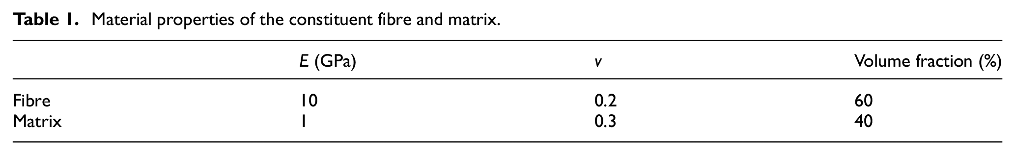
An independent validation was conducted against results obtained from FEM. The present forward analysis was applied to the composite of constituent properties in Table 1 as quoted from the study by Li and colleagues [6,9], with results presented in Table 2. Although the composite analysed here is a hypothetic one, there is a complete set of output data available in the literature obtained independently through a different means, FEM, and therefore, the comparison of the results should offer a reasonable case of validation.

Table 1.

Material properties of the constituent fibre and matrix.

	E (GPa)	v	Volume fraction (%)
Fibre	10	0.2	60
Matrix	1	0.3	40

Table 2.

Effective material properties of the composite.

		Square unit cell	Hexagonal unit cell
Longitudinal Young’s modulus	Ez (GPa)	6.4034 (6.4033)	6.4030 (6.4029)
Transverse Young’s modulus	Ex = Ey (GPa)	3.2952 (3.2951)	2.8550 (2.8552)
Transverse shear modulus	Gxy (GPa)	0.91439 (0.91441)	1.0823 (1.0824)
Longitudinal shear modulus	Gxz = Gyz (GPa)	1.1948 (1.1948)	1.1531 (1.1533)
Major Poisson’s ratio in fibre direction	vzx = vzy	0.23234 (0.23234)	0.23337 (0.23337)
Poisson’s ratio in transverse direction	vxy	0.22970 (0.22974)	0.31899 (0.31896)

Values included in brackets were quoted from the study by Li and Sitnikova [5,6].

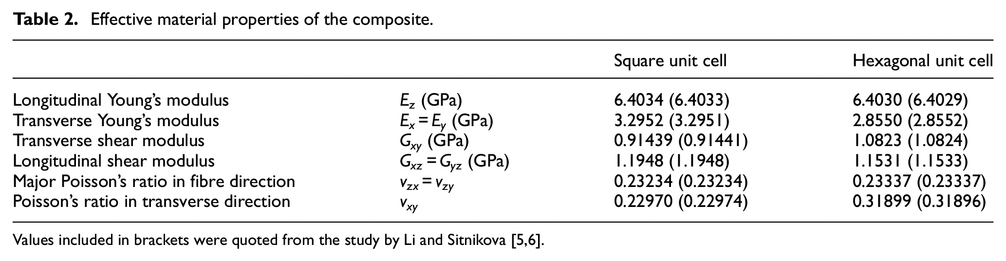
It can be seen that the present analysis almost reproduced the results in the study by Li and colleagues [6,9] exactly and any difference took place at the fifth effective digit. The present forward analysis has comfortably passed this round of validation. It should be stated that the current results should be closer to the exact solution while the results from FEM as shown in brackets could be improved slightly if the mesh employed there was refined, though sufficiently converged already, the outcome would move closer to the present results. Of course, the so-called differences here were tiny and offered as a means of verification and validation of the analysis rather than any practical significance. The CPU time consumed using the present analysis was much lower than that using FEM. It is less a second to run on the authors’ laptop. This is particularly important for the subsequent iterative analysis involved in the inverse problem. The most important point is that the analysis can be run on a platform, MATLAB, where the forward problem can be built seamlessly into a code as the subsequent development for the inverse problem.

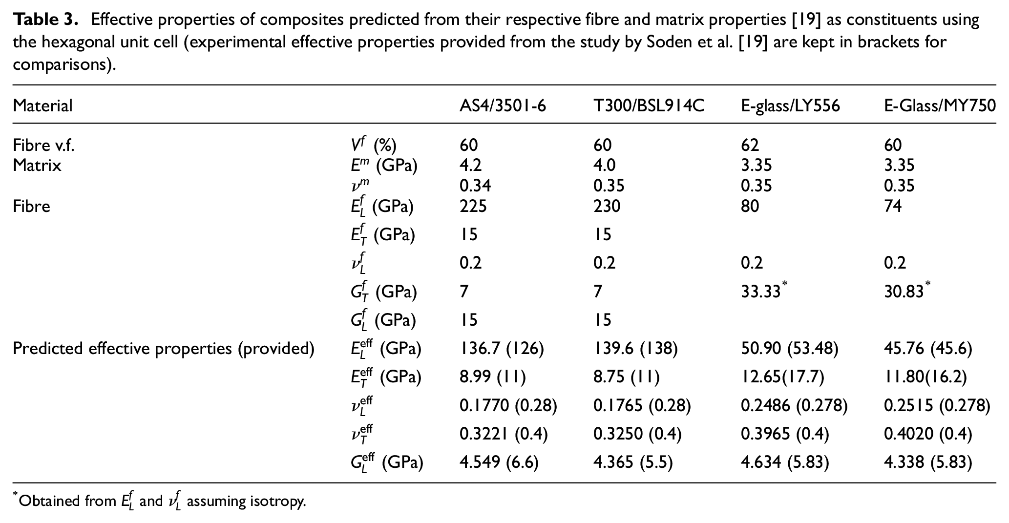
The present analysis has been validated against four sets of experimental data from four different composites, two of carbon fibres and two of glass fibres. These composites were employed in the World-Wide Failure Exercise [19] where properties of fibre and matrix were both provided as listed in Table 3. They have been used to predict the effective properties of the composites, which are also presented in Table 3 and compared with the experimental values as provided in the study by Soden et al. [19], included in Table 3 in brackets.

Table 3.

Effective properties of composites predicted from their respective fibre and matrix properties [19] as constituents using the hexagonal unit cell (experimental effective properties provided from the study by Soden et al. [19] are kept in brackets for comparisons).

Material		AS4/3501-6	T300/BSL914C	E-glass/LY556	E-Glass/MY750
Fibre v.f.	$V^f$ (%)	60	60	62	60
Matrix	$E^m$ (GPa)	4.2	4.0	3.35	3.35
	${\nu }^m$	0.34	0.35	0.35	0.35
Fibre	$E_L^f$ (GPa)	225	230	80	74
	$E_T^f$ (GPa)	15	15
	${\nu }_L^f$	0.2	0.2	0.2	0.2
	$G_T^f$ (GPa)	7	7	33.33 *	30.83 *
	$G_L^f$ (GPa)	15	15
Predicted effective properties (provided)	$E_L^{\mathrm{eff}}$ (GPa)	136.7 (126)	139.6 (138)	50.90 (53.48)	45.76 (45.6)
	$E_T^{\mathrm{eff}}$ (GPa)	8.99 (11)	8.75 (11)	12.65(17.7)	11.80(16.2)
	${\nu }_L^{\mathrm{eff}}$	0.1770 (0.28)	0.1765 (0.28)	0.2486 (0.278)	0.2515 (0.278)
	${\nu }_T^{\mathrm{eff}}$	0.3221 (0.4)	0.3250 (0.4)	0.3965 (0.4)	0.4020 (0.4)
	$G_L^{\mathrm{eff}}$ (GPa)	4.549 (6.6)	4.365 (5.5)	4.634 (5.83)	4.338 (5.83)

*

Obtained from $E_L^f$ and ${\nu }_L^f$ assuming isotropy.

To support the validation, the results presented in Table 3 are discussed as follows. While agreements can be observed in many places, main discrepancies are found in the following three aspects:

1. The transverse Young’s moduli were underpredicted for all composites. While the regular packing of fibres in the composites as assumed through the use of a unit cell has the tendency of leading to a lower transverse Young’s modulus, as discussed in the study by Wongsto and Li [20], this particular property is usually of a much lower magnitude than its longitudinal counterpart and hence prone to measurement errors practically. This is also exacerbated by the moderate nonlinear behaviour in the transverse direction.

2. The transverse Poisson’ ratios ${\nu }_T^{\mathrm{eff}}$ for both carbon fibre composites were substantially lower than the provided values. This was primarily due to the input value of ${\nu }_T^f$ , which was 0.071 as derived from the transverse properties of the fibre $E_T^f$ and $G_T^f$ provided in the study by Soden et al. [19], assuming transverse isotropy as was commonly accepted for carbon fibres, as opposed to its typical value around 0.2 [4].

3. The discrepancy in along-fibre shear moduli $G_L^{\mathrm{eff}}$ is also pronounced. This particular property is, in general, highly nonlinear. The provided value was meant to be the initial modulus but the measurement errors are inevitable for the initial stage at very low load levels. Typically, some artificial treatments have to be made to locate the origin of stress–strain curve. In fact, for some of the composites involved, even if the fibre shear modulus was assumed to be infinitely large, that is rigid, the unit cell would still not be able to reach an effective shear modulus as high as provided in the study by Soden et al. [19].

The commonality among the above three aspects of disagreement points to the quality of the experimental data available, both the properties of constituents as the input and the effective properties of the composite for the output to compare with. It is understandable that many of such properties are difficult to measure practically. Some kind of assessment of the quality of these data would be helpful. This is certainly a desirable development worthwhile to explore in future.

3. The inverse problem for the fibre properties

The so-called inverse problem for unit cells is to extract the properties of the fibre from the effective properties of the composite represented by the unit cell, given the properties of the matrix involved. If some of the properties of the fibre are known, then the extraction can be for the remaining unknown ones.

In much the same way as nonlinear problems being solved through a series of linear analyses, the inverse problem can also be solved through a series of forward problems, starting from a set of estimated fibre properties to obtain their corresponding effective properties of the composite. Comparing these effective properties with those measured experimentally, assessment can be given to the estimated fibre properties and improvement can be suggested for the next iteration. The iterations carry on until the obtained effective properties are sufficiently close to the experimental values.

A practical way of facilitating the iterative process described above is to formulate it into an optimisation problem. The sum of the square of relative errors in the predicted effective properties of the composite with respect to the provided counterparts can be taken as the objective function which is non-negative in nature, with all fibre properties to be found as the optimisation variables. Apart from basic restrictions, such as non-negative optimisation variables in this case, there is no other constraint, which simplifies the current optimisation problem greatly. The relative errors included in the objective function can be weighted, so that the accuracies of each measured effective property of the composites can be taken into account. Relatively, the measurement of the effective Young’s modulus and the Poisson’s ratio in fibre direction is the most reliable, those in the transverse direction next. The along-fibre direction shear modulus cannot be measured as reliably as the previously mentioned ones. One of the reasons is the significant nonlinearity as observed in this respect of composite behaviour. A rational approach of formulating such a nonlinear problem was addressed recently in the study by Li et al. [21]. The shear modulus in the plane transverse to fibres is most unreliable and the test standard is perhaps the least established. As a result, the provided values are bound to be the least reliable. However, if such variability is to be taken into consideration, detailed experimental data, such as the standard deviations, should be available, which is hardly the case from the data in the open literature. Otherwise, one can always assign a weight of 1 to all of them to facilitate the analysis.

The objective function for optimisation can therefore be defined as:

$$\mathrm{\Pi }\left(\mathbf{p}\right)=\sum _{j=1}^5{W}_j\frac{{(Q_j^{\mathrm{e}\mathrm{ff}}\left(\mathbf{p}\right)-Q_j^{\exp })}^2}{{Q_j^{*}}^2}$$

(43)

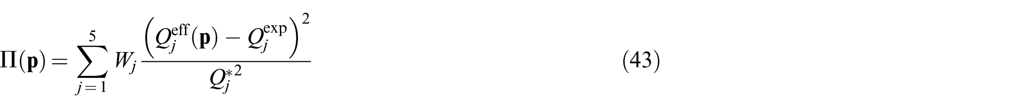
where Q_j^eff is one of the effective composite properties predicted from the unit cell, Q_j^exp is the corresponding effective properties as provided, and W_j is the weight assigned to this property. There are five of such properties for transversely isotropic composites in general. Fibre properties to be found are denoted as p which defines the optimisation variable vector and there can be up to five components in it.

An optimisation routine, fmincon, in MATLAB can be resorted. In the present case, there is no constraint. However, to run it, like most of the optimisers, a set of initial values for the optimisation variables is required. For this purpose, the Halpin–Tsai formula [4] can be resorted to, which tends to produce reasonably reliable prediction of effective properties while remaining simple and analytical. It is employed to produce initial values as follows. The expression for $E_L^f$ and ${\nu }_L^f$ can be obtained from,

$$P^f=\frac{1}{V^f}(P^{\mathrm{eff}}-(1-V^f)P^m)$$

(44)

with $P^f$ being $E_L^f$ and ${\nu }_L^f$ , $P^{\mathrm{eff}}$ and $P^m$ are the corresponding effective property of the composite and the matrix property, respectively, and V ^f is the fibre volume fraction as previously introduced. The remaining fibre properties, that is, transverse Young’s modulus $E_T^f$ , Poisson’s ratio ${\nu }_T^f$ , and along-fibre shear modulus $G_L^f$ , should be obtained from,

$$P^f=P^m\frac{P^m\xi V^m-P^{\mathrm{eff}}(\xi +V^f)}{P^{\mathrm{eff}}{V}^m-P^m(1+\xi V^f)}$$

(45)

where parameter ξ is mostly a fudge factor and its recommended value of 1 was taken. It should be pointed out that the above obtained initial values are not always sensible, although the Halpin–Tsai formula in the forward prediction is quite reasonable. Sometimes, negative values could be produced from equation (45), which usually corresponds to a case in which significant inconsistency was present in the effective properties involved. In this case, the corresponding initial value is readjusted as follows:

$$P^f=\frac{P^{\mathrm{eff}}}{V^f}.$$

(46)

In addition to the initial values, a set of upper and lower bounds is also required for the variables. They can be obtained from the initial value by adding and subtracting an increment associated with the initial values, respectively. In general, for initial values obtained from equation (46), more generous increment sizes should be considered.

It should be pointed out that the initial values, and the bounds, while affecting convergence, make difference to the converged solution. In this sense, there is a certain arbitrariness in the selection of the initial values and the bounds. It is the users’ responsibility to give the obtained solution some basic assessment to confirm whether the results are reasonable, if necessary, attempting a few different combinations, as a typical verification process is essential in most numerical approaches. Fortunately, based on a sizable range of parametric study conducted by the authors, within a substantial neighbourhood of a reasonable solution, there is no other local minima of the objective function as another solution to the optimisation problem. In other words, the converged solution is either reasonable or obviously unreasonable. In the latter case, the initial values and the corresponding bounds will have to be adjusted.

In the forward problem, the analyses in the plane of the cross-section and that out of this plane are decoupled and therefore they can also be dealt with separately in the inverse problem, which should help the convergence. For the problem in the plane of the cross-section, the objective function can be written, after setting all the weights to 1, as

$${\mathrm{\Pi }}_{\mathrm{in}-\mathrm{plane}}\left(\mathbf{p}\right)=\frac{{(E_L^{\mathrm{e}\mathrm{ff}}\left(\mathbf{p}\right)-E_L^{\exp })}^2}{{\left(E_L^{\exp }\right)}^2}+\frac{{({\nu }_L^{\mathrm{e}\mathrm{ff}}\left(\mathbf{p}\right)-{\nu }_L^{\exp })}^2}{{\left({\nu }_L^{\exp }\right)}^2}+\frac{{(E_T^{\mathrm{e}\mathrm{ff}}\left(\mathbf{p}\right)-E_T^{\exp })}^2}{{\left(E_T^{\exp }\right)}^2}+\frac{{({\nu }_T^{\mathrm{e}\mathrm{ff}}\left(\mathbf{p}\right)-{\nu }_T^{\exp })}^2}{{\left({\nu }_T^{\exp }\right)}^2}$$

(47)

where $\mathbf{p}={\left[\begin{array}{cccc}{E}_L^f\hfill & {\nu }_L^f\hfill & E_T^f\hfill & {\nu }_T^f\hfill \end{array}\right]}^T$ are the variables. It can include all four variables, or, in some cases, if some of them, for example, $E_L^f$ , are provided by manufacturer, then the number of independent variables will reduce. Alternatively, if the fibre is known to be isotropic, then there will be a reduction in the number of independent variables. However, no matter how many independent variables are involved, the four terms involved in the objective function must be kept, as each of the effective properties can be affected by the values of all remaining independent variables.

For the part out of the plane of the cross-section of the composite, there is only one variable and the objective function can be given as:

$${\mathrm{\Pi }}_{\mathrm{out}-\mathrm{of}-\mathrm{plane}}\left(G_L^f\right)=\frac{{(G_L^{\mathrm{e}\mathrm{ff}}\left(G_L^f\right)-G_L^{\exp })}^2}{{\left(G_L^{\exp }\right)}^2}.$$

(48)

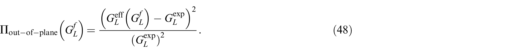
It is a similar but simpler problem than its in-plane counterpart above.

4. Verification and validation of the inverse analysis

The inverse problem is verified and validated in this section by applying it to a number of problems. For the sake of representativeness, the hexagonal unit cell will be employed in the subsequent analyses since all composites to be dealt with fall into the category of transverse isotropy.

As a verification of the inverse problem, the effective properties as shown in Table 2 and the matrix properties as given in Table 1 were employed as the input data to the minimisation of equations (47) or (48). Out of the inverse analysis, fibre properties were predicted. Comparing with those provided in Table 1, an accuracy of 99.9% was achieved, corresponding to a virtually vanishing value of the objective function. The negligible disparity was mainly due to the truncation error of the effective properties shown in Table 2 as the input data.

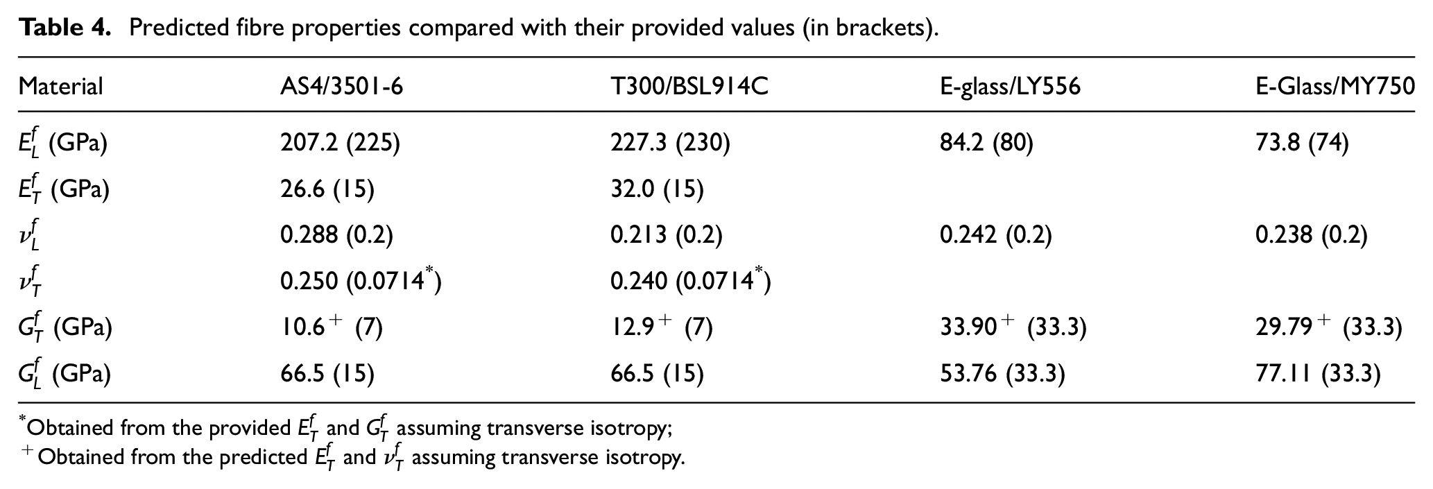
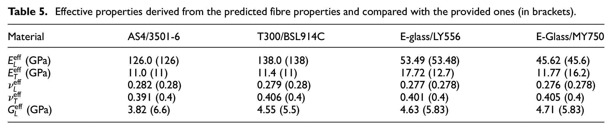
After successful verification above, the inverse analysis was applied to the set of composites as included in Table 3 quoted from the study by Soden et al. [19] for the purpose of validating the inverse analysis. The effective properties along with their respective matrix properties as the experimental data provided in the study by Soden et al. [19] as listed in Table 3 were used as the input. For the given input data, the predicted fibre properties are presented in Table 4 and compared with those provided [19] in brackets next to their predicted counterparts. To help with the discussion of the results, in particular, the evaluation of the quality of the input data, the effective properties derived (through a forward analysis) from the predicted fibre properties (output of the inverse analysis) are presented in Table 5.

Table 4.

Predicted fibre properties compared with their provided values (in brackets).

Material	AS4/3501-6	T300/BSL914C	E-glass/LY556	E-Glass/MY750
$E_L^f$ (GPa)	207.2 (225)	227.3 (230)	84.2 (80)	73.8 (74)
$E_T^f$ (GPa)	26.6 (15)	32.0 (15)
${\nu }_L^f$	0.288 (0.2)	0.213 (0.2)	0.242 (0.2)	0.238 (0.2)
${\nu }_T^f$	0.250 (0.0714 * )	0.240 (0.0714 * )
$G_T^f$ (GPa)	10.6 + (7)	12.9 + (7)	33.90 + (33.3)	29.79 + (33.3)
$G_L^f$ (GPa)	66.5 (15)	66.5 (15)	53.76 (33.3)	77.11 (33.3)

*

Obtained from the provided $E_T^f$ and $G_T^f$ assuming transverse isotropy;

+

Obtained from the predicted $E_T^f$ and ${\nu }_T^f$ assuming transverse isotropy.

Table 5.

Effective properties derived from the predicted fibre properties and compared with the provided ones (in brackets).

Material	AS4/3501-6	T300/BSL914C	E-glass/LY556	E-Glass/MY750
$E_L^{\mathrm{eff}}$ (GPa)	126.0 (126)	138.0 (138)	53.49 (53.48)	45.62 (45.6)
$E_T^{\mathrm{eff}}$ (GPa)	11.0 (11)	11.4 (11)	17.72 (12.7)	11.77 (16.2)
${\nu }_L^{\mathrm{eff}}$	0.282 (0.28)	0.279 (0.28)	0.277 (0.278)	0.276 (0.278)
${\nu }_T^{\mathrm{eff}}$	0.391 (0.4)	0.406 (0.4)	0.401 (0.4)	0.405 (0.4)
$G_L^{\mathrm{eff}}$ (GPa)	3.82 (6.6)	4.55 (5.5)	4.63 (5.83)	4.71 (5.83)

The agreements and disagreements are discussed as follows. Excellent agreement can be observed in many aspects, but significant discrepancies can be found again in three aspects directly associated with those discussed in the forward analysis as discussed in subsection 2.8 and for the same reasons:

1. The transverse Young’s moduli $E_T^f$ of the fibre were overpredicted for all composites because of the high transverse effective Young’s modulus of the composite, which is not the easiest property of the composite to be measured accurately.

2. The transverse Poisson’s ratios ${\nu }_T^f$ of the carbon fibres are substantially higher that the indirectly provided values (worked out from the transverse shear modulus assuming transverse isotropy), which was in fact not representative at all for typical carbon fibres. In this case, the predicted value from the inverse analysis is definitely more representative than the provided values. The disagreement in transverse shear modulus $G_T^f$ is a natural consequence of those in $E_T^f$ and ${\nu }_T^f$ , given the transverse isotropy for fibres.

3. The predicted along-fibre shear moduli $G_L^f$ from the inverse analysis are significantly higher than the provided values. This was because of excessively high values of the transverse effective Young’s modulus of the composite as provided was used as the input to the inverse analysis. Even with such overestimated $G_L^f$ , if it is employed in a forward analysis, it would not be able to generate effective longitudinal shear moduli as high as provided ones, as shown in Table 5. It can be concluded that the provided effective longitudinal shear moduli were not quite representative for the composites concerned.

From Table 5, it can be concluded that, except for $G_L^f$ , other predicted fibre properties as given in Table 4 tend to be more representative than the provided ones for the composites, as they could produce effective properties more closely to the provided counterparts (in brackets). It is not difficult to conclude that among the provided fibre properties from the study by Soden et al. [19], significant mismatch was present between $E_T^f$ and $G_T^f$ for leaving an unrealistic ${\nu }_T^f$ (not provided directly but available from isotropy). Also the provided composite effective property $G_L^{\exp }$ was generally unrealistically high, which could not be achieved even if the fibres became rigid.

5. Discussion on the formulation and applicability

The work as presented in this paper was motivated by the fact that for many types of composites, the properties of the fibres employed are found incomplete in the literature and there is no readily tangible means to measure them. As a result, offering an accessible means to evaluate those missing properties is helpful. This paper does exactly this based on the readily available data, including the properties of the matrix and the effective properties of the composite.

As in many other similar analyses, a number of basic assumptions have been made to allow the complicated reality to be idealised into a theoretical model as dealt with in this paper. They are summarised here. In the UD composite, fibres lie in the direction along the z-axis perfectly straight, which will justify a 2D presentation of the problem to be formulated. They are of an identical circular cross-section. Over the cross-section of the composite, fibres are regularly packed into a square or hexagonal array. The use of a unit cell of square or hexagonal shape can be justified accordingly. Between fibre and matrix, there is perfect bonding so that the continuity in displacement and traction across the interface can be assumed. The diameter of the fibre is much smaller than its longitudinal dimension. Thus, under macroscopically uniform loading conditions, the microscopic deformation can be idealised into a GPE problem. The fibre is transversely isotropic and the matrix isotropic. They are both linearly elastic. As the objective is to characterise elastic properties of fibres, deformation can always be kept small, so that the theory of elasticity under small deformation applies. While the listed assumptions might sound rather restrictive, they actually have a reasonable range of applicability. A minor degree of deviation from the assumed positions may not necessarily cause excessive differences in general. Having said so, due care needs to be exercised to avoid any abuse of them.

The forward problem is in fact a material characterisation tool for UD composites using unit cells. When solved using complex potentials, the solution turns out to be fairly simple and systematic. Relevant codes in MATLAB are provided as a part of this paper in the form of companion data. Interested readers are welcome to take advantage of them.

Inverse problems are typically ill-posed, as was also recognised in the study by Nanthakumar et al. [11]. For a given set of input data, there does not always exist an exact solution which would reproduce the input data from the forward analysis. By turning the inverse problem into an optimisation problem, it eases the difficulty greatly in the sense that it seeks a solution which minimises, instead of eliminating, the error. Inconsistent input data would exacerbate the ill-posed nature of the problem to be solved, resulting in excessive error as reflected by the high value of the objective function after convergence. Sometimes, the iterations might find difficulties to convergence. Relevant codes in MATLAB are also provided as a part of this paper in the form of companion data. Their use should always be mindful of the consistency of the input data.

From the verification case for the inverse problem, it is clear that a precise result can be obtained from the input data provided that a solution exists corresponding to the input data. In other words, if the solution (fibre properties) from the inverse analysis is used in the forward analysis, it reproduces the input data (effective properties of the composite). Such input data are considered as perfectly consistent ones. Parametric studies indicate that the inverse analysis is sensitive to the input data. It is important that the input data to be employed in practical applications are at least qualitatively consistent.

In practical applications, the input data available are usually not as consistent as one would like, in which case the solution can only be approximate if found and sometimes a solution may not even be found. Examples of inconsistent properties can be found in those provided in the study by Soden et al. [19] in both fibre properties and composite effective properties. For instance, $E_T^f$ and $G_T^f$ for both carbon composites did not seem to match, as the transverse Poisson’s ration ${\nu }_L^f$ would be 0.071 which was far from to its typical range around 0.2 [4]. The effective longitudinal shear modulus $G_L^{\exp }$ provided in the study by Soden et al. [19] for each of the four composites was generally unrealistically high, which could not be achieved using whatever fibres at the given fibre volume fraction. It is clear that inconsistent data are not unusual in the open literature and due diligence is users’ responsibility. The consistency in the input data should not be taken for granted simply because they are perceived to be “experimentally measured.”

While the achievement made by this paper sets a milestone in this direction, more efforts are required to bring this approach forward to become a practical tool for relevant users. A crucial aspect would be the quality assessment of the input data to the inverse analysis. It can be envisaged that as a future development that some kind of correction system will be put forward when such data are generated from relevant experiments.

6. Conclusion

A semi-analytical micromechanical analysis has been formulated based on a square or hexagonal unit cell using the complex function solution under a GPE condition as the forward problem. As the outcome of the analysis, the average stresses and strains in the unit cell can be found, from which the effective properties of the composite represented by the unit cell can be obtained. The validity and accuracy of the forward analysis have been convincingly established through the verifications conducted. Its applicability to practical problems has been demonstrated through validation where four different types of real composites have been considered with the results compared with those experimentally obtained ones. Reasonable agreements have been shown in section 2.

As the inverse problem to its forward counterpart, the fibre properties can be evaluated from the effective properties of the composite and the properties of the matrix as the other constituents of the composite. It has been formulated as an optimisation problem to minimise the difference between the predicted effective properties and the provided ones experimentally measured. The validity of the inverse problem has been verified by reproducing fibre properties from the composite effective properties derived from forward analysis. Practical applications of the inverse problem as the validation exercise have revealed two important and related aspects. In the presence of consistent effective properties of the composite, reasonable fibre properties can usually be predicted satisfactorily. In cases where unreasonable fibre properties are produced, or sometimes, the optimisation iterations fail to converge, they are usually associated with scenarios in which effective properties of the composites are out of step significantly and hence inconsistent. In this case, appropriate review needs to be given to the measured effective properties of the composites before they are put into a meaningful inverse analysis. This has been argued appropriately in section 4 and further discussed in section 5.