In this paper, we study the well-posedness of a class of evolutionary variational–hemivariational inequalities coupled with a nonlinear ordinary differential equation in Banach spaces. The proof is based on an iterative approximation scheme showing that the problem has a unique mild solution. In addition, we established the continuity of the flow map with respect to the initial data. Under the general framework, we consider two new applications for modeling of frictional contact for viscoelastic materials. In the first application, we consider Coulomb’s friction with normal compliance, and in the second, normal damped response. The structure of the friction coefficient is new with motivation from geophysical applications in earth sciences with dependence on an external state variable and the slip rate .
This work concerns the study of an evolutionary differential variational–hemivariational inequality modeling mathematical problems from contact mechanics. These systems are relevant for many physical phenomena ranging from engineering to biology (see, e.g., [1–3] and the references therein). We are interested in frictional contact phenomena for viscoelastic materials with the linearized strain tensor, which have been studied intensively (see, e.g., some of the relevant books [2–4]).
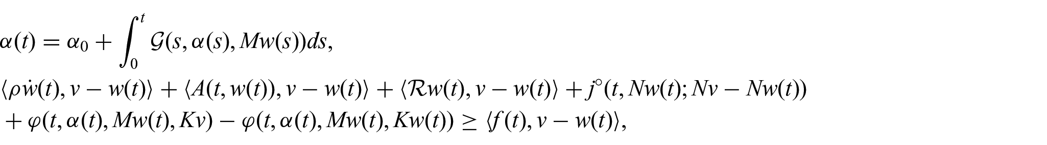
Let and be two Banach spaces, and for , we let be the time interval of interest. Then, the Cauchy problem under consideration reads:
for all , a.e. with
Here, and are the nonlinear operators related to the viscoelastic constitutive laws. Furthermore, is a generalized directional derivative of a functional . The functionals and are determined by contact boundary conditions. We require to be convex in its last argument, while may be nonconvex with appropriate structures given later (see Section 3). The operators and relate to the contact conditions, and is assumed to be a nonlinear operator related to the change in the external state variable . The data is related to the given body forces and surface traction, and and represent the initial data. Finally, , , and are the bounded linear operators related to the tangential and normal trace operators. The Cauchy problem (1b) and (1c) is called a hemivariational inequality if and variational inequality if . Moreover, a solution to equation (1) is understood in the mild sense.
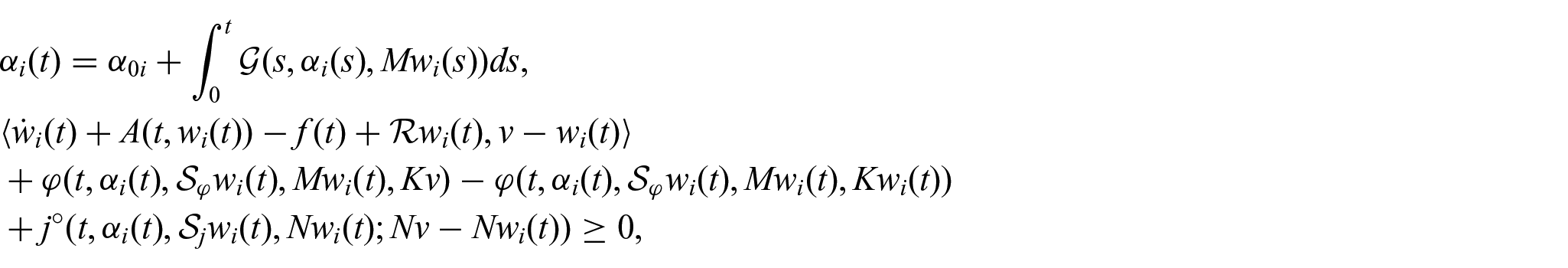
Definition 1.A pair of functions , where and measurable, is said to be a mild solution of equation (1) if and , respectively, satisfy:
The main purpose of this paper is to extend the results from Migórski [5] and Pătrulescu and Sofonea [6] to prove well-posedness of equation (1) with applications to rate-and-state frictional contact problems. We prove that the pair is a solution to equation (1) in the sense of Definition 1 and that the flow map depends continuously on the initial data. The problem setting is motivated by Shillor et al. [3], Pătrulescu and Sofonea [6], Pipping [7], Sofonea and Migórski [8], and the techniques have taken inspiration from Migórski and Bai [9].
1.1. Former well-posedness results
Special cases of equation (1) have been investigated in the literature. The recent work [5] is closest to our setting. They prove well-posedness for an ordinary differential equation (ODE) coupled with a variational–hemivariational inequality with applications to viscoplastic material and viscoelasticity with adhesion. In fact, if we let be independent of in its third argument and relax the more generalized structure of (see Remark 4 for more details), then equation (1) reduces to the problem studied in Migórski [5]. However, keeping the dependence of in and a generalized structure of (see Remark 4) allows us to include applications with a new structure of the friction coefficient. On the contrary, neglecting and in and in , existence and uniqueness are provided in Sofonea and Migórski [8, Section 10.3]. If we let and be independent of and , existence and uniqueness were proved in Han and Sofonea [10, Section 6].
In the quasi-static case tackled in Pătrulescu and Sofonea [6] with and a simplified structure of (see Remark 4), they proved existence and uniqueness of the solution pair by an implicit method, where they rewrite equation (1a) to only depend on . However, the setting of Pătrulescu and Sofonea [6] is not applicable in our case as the inertial term restricts the space-time regularity for . We refer to Migórski [5, p. 2] for further discussion.
1.2. Physical setting
A mathematical model in contact mechanics needs several relations: a constitutive law, a balance equation, boundary conditions, interface laws, and initial conditions. The constitutive laws help us describe the material’s mechanical reactions (stress–strain type). In most cases, constitutive laws originate from experiments, although they are verified to satisfy certain invariance principles. We refer to Han and Sofonea [11, Chapter 6] for a general description of several diagnostic experiments which provide the needed information to construct constitutive laws for specific materials. The interface laws are prescribed on the possible contact surface. We refer to the interface laws in tangential direction as friction laws and in normal direction as contact conditions. The mathematical treatment of these problems gives rise to the variational–hemivariational inequalities of the form equations (1b) and (1c), where we put appropriate constraints on the operators to fit the applications of interest.
We are mainly interested in studying frictional problems with the following dependencies:
One application with the dependencies seen in equation (2) is a memory-dependent friction coefficient (see, e.g., [12, Section 5.3]), which is also referred to as rate-and-state friction law. This is modeled via an ODE, where the state variable tracks information of the contact surface using the slip rate found from solving equations (1b) and (1c) and then updates the friction coefficient. Under certain constraints, we may consider as the surface temperature or humidity on the contact surface.
In Pătrulescu and Sofonea [6], they assume that is bounded and Lipschitz with respect to both arguments. In addition to the boundeness assumption on the friction coefficient, Migórski [5] considers applications in the frictionless setting and . Our framework is therefore an extension of the frameworks in Migórski [5], Pătrulescu and Sofonea [6], where we need to use different techniques to prove the well-posedness of equation (1) in the sense of Definition 1. Finally, is covered in [4, Sections 6.3 and 8.1] (see also [10, p. 185–187]). A discussion on many different friction models can be found in Zmitrowicz [13].
1.3. Contributions and outline
The novelties of this paper are as follows:
Well-posedness of equation (1) in the sense of Definition 1, where the proof is based on an iterative decoupling approach that directly gives rise to a numerical method.
A more complicated structure of (see Remark 4) that allows for a larger set of conditions on the contact surface.
Two new applications with Coulomb’s friction. One contact problem is with normal compliance, and the latter is with normal damped response. The general framework allows a new structure for the friction coefficient that can be unbounded.
This paper is organized as follows. In Section 2, we introduce the function spaces and some basics of nonsmooth analysis in order to better understand the problem setting. In Section 3, we present our problem statement and the assumptions on the data. The section ends with our main result, Theorem 2, that summarizes the well-posedness of equation (1) in the sense of Definition 1. The proof of the theorem is presented in Section 5 utilizing a preliminary result stated in Section 4. Next, two applications fitting our framework will be introduced in Sections 6.1 and 6.2. In Section 6.3, we introduce an application motivated by earth sciences. Finally, in Appendix 1, we include remarks on the assumptions needed in the proof of Theorems 2, 4, and 5. Appendices 2–7 contain proofs of results that are similar to ones found elsewhere but needed throughout this paper.
1.4. Notation
We now present some notations that will be used in this paper.
Let be the maximal time.
Let denote the dimension. In the applications, .
A point in is denoted by , .
denotes the space of second-order symmetric tensors on .
We denote |·| as the Euclidean norm.
is a bounded open connected subset with a Lipschitz boundary . We split into three disjoint parts; , , and with , , i.e., nonzero Lebesgue measure, but is allowed to be empty.
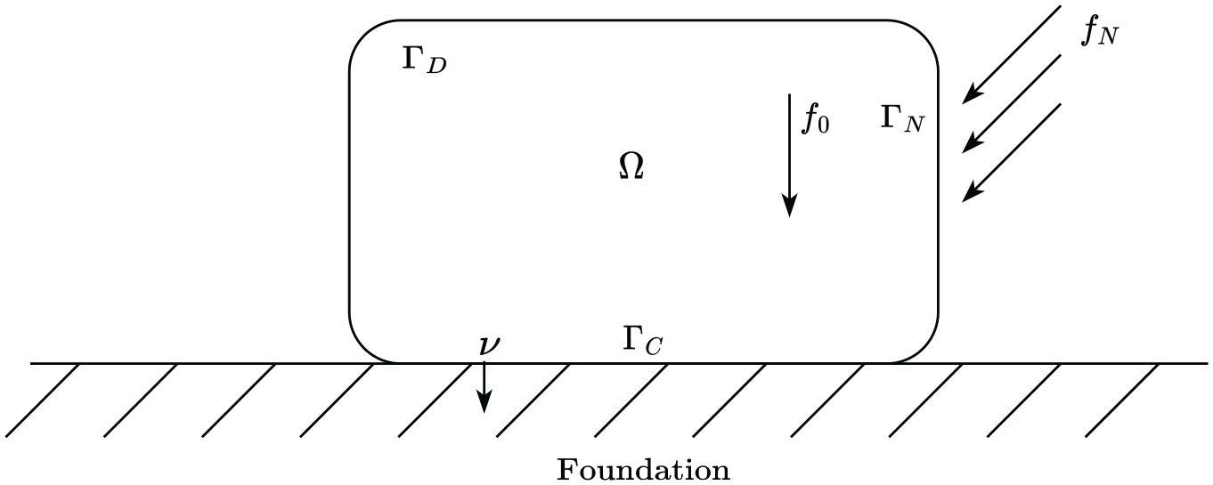
In the applications, is the reference configuration of a viscoelastic deformable body sliding on a foundation. Moreover, denotes the Dirichlet boundary, the Neumann boundary, and is the contact boundary.
denotes the outward normal on .
We denote .
denotes the space of Lebesgue -integrable functions equipped with the norm for . With the usual modifications for .
denotes the space of infinitely differentiable functions with compact support.
We will denote as a positive constant, which might change from line to line.
Let be a function, then we denote the time derivative of by and the double time derivative as . Assuming here that has enough regularity such that it makes sense to take the time derivative of it twice.
and denote the arbitrary (separable reflexive) Banach spaces. For the convenience of the reader, this notation will be used when introducing general theory. If the theory is only needed for a specific (separable reflexive) Banach space, we write the specific space.
The dual space of will be denoted by .
denotes the set containing all subsets of .
The dual product between the spaces and will be denoted by .
In the particular case, when is an inner product space, we denote as its inner product.
, , , , and denote the real separable reflexive Banach spaces, and is a real Hilbert space.
The embedding is referred to as an evolution triple. Here, the embedding is continuous and dense in . It follows that is continuously embedded (see, e.g., [14, Section 7.2]). Moreover, is compactly embedded, leading to being compactly embedded (see,e.g., [15, Remark 3.4.4]).
For simplicity of notation, the dual product between and is denoted by .
denotes the set of all bounded linear maps from into .
We denote the operator norm of the operators , , and as , , and , respectively.
2. Function spaces and basics of nonsmooth analysis
In this section, we present the function spaces and fundamental results. For further information, we refer to standard textbooks, e.g., Roubíček [14], Cheney [16], Evans [17], and Pedersen [18].
2.1. Sobolev spaces
This section defines the solution spaces and the usual Sobolev spaces, which will become useful in Section 3 and in the applications, i.e., Section 6. We define:
for . The associated norms will be denoted and , respectively. For , equations (3) and (4) are Hilbert spaces with the canonical inner products:
for all , . Moreover, we define the spaces:
and
With abuse of notation, the trace of functions on will still be denoted by . For the displacement, we use the space:
As a consequence of , it follows by Korn’s inequality, i.e., (see, e.g., [19, Lemma 6.2]), that is a Hilbert space with the canonical inner product:
Here, is the deformation operator defined by:
We denote the associated norm on by . Moreover, if is a regular function, say , the following Green’s formula holds:
We also need the following trace theorem from Adams and Fournier [20, Theorem 4.12].
Theorem 1.Let be bounded with Lipschitz boundary and be such that . Then, there exists a linear continuous operator satisfying:
for all. If, then. And, .
We denote as a Cartesian product space, for some , where are normed spaces for . Then, is equipped with the norm:
Equivalently, we may equip with the norm:
2.2. Time-dependent spaces
Let be an evolution triple.
Definition 2.Let be a Banach space, and . The space , , consists of all measurable functions such that:
With the usual modifications for. For brevity, we use the standard short-hand notation:
for all and.
We also introduce the solution space:
equipped with the norm . The duality pairing between and is denoted by:
We denote the space of continuous functions defined on with values in by:
The next proposition can be found in, e.g., Denkowski et al. [15, Proposition 3.4.14] or Roubíček [14, Lemma 7.3] and will help us provide estimates.
Proposition 1.Let be an evolution triple in space, and . Then, for any (defined in equation (7)), and for all , the following integration by parts formula holds:
In addition, the embeddingis continuous.
For more on evolution spaces and other time-dependent spaces, which are also referred to as Bochner spaces, see, e.g., Roubíček [14, Chapter 7], Denkowski et al. [15, Section 3.4], Zeidler [21, Chapter 23], Yosida [22, Chapter V, Section 5], or Evans [17, Section 5.9.2 and Appendix E.5].
We finally introduce the following Bochner space needed in the applications, i.e., in Section 6.
Definition 3.Let be a real Banach space, then the Bochner space consists of all functions such that exists in the weak sense and belongs to . The space is equipped with the norm:
2.3. Generalized gradients
Let be a reflexive Banach space. In contact mechanics, we are often interested in contact conditions of the form , where represents an interface force, the normal component of the displacement, and being the Clarke subdifferential of defined as below.
Definition 4.Let be a locally Lipschitz function. The generalized (Clarke) directional derivative of at in the direction , denoted , is defined by:
Moreover, the subdifferential in the sense of Clarke ofat, denoted , is a subset of of the form:
Remark 1.To say that a function is locally Lipschitz on means that is Lipschitz continuous in a neighborhood of .
Remark 2.We refer the reader to, e.g., Han and Sofonea [10, p. 185–187] and Migórski et al. [4, Section 6.3] for examples related to contact mechanics. Other examples may be found in, e.g., Clarke [23] and Denkowski et al. [24].
Proposition 2.Let be a Banach space and be locally Lipschitz on . Then, is upper semicontinuous.
Proposition 3.Let be a Banach space. If is proper, convex, and lower semicontinuous, then is locally Lipschitz on the interior of the domain of.
Proposition 2 can be found in Denkowski et al. [24, Proposition 5.6.6], and Proposition 3 can be found in Denkowski et al. [24, Proposition 5.2.10].
Definition 5.Let be a proper and convex function. The (generally multivalued) mapping , written:
is called the convex subdifferential ofat.
Proposition 4.Let be locally Lipschitz on . If is convex, then coincides with .
The proof of the above proposition is found in Clarke [23, Proposition 2.2.7]. Finally, to show that is indeed a solution to Problem 1 (see Section 3), we require the following result found in Migórski et al. [4, Lemma 3.43].
Lemma 1.Let and be two Banach spaces and be such that:
(1)is continuous onfor all.
(2)is locally Lipschitz on for all .
(3) There exists such that for all , we have:
where denotes the generalized gradient of.
Then, is continuous on .
To read more on the generalized directional derivatives, subdifferential, and nonsmooth analysis, see, e.g., Clarke [23, Chapter 2], Denkowski et al. [24, Chapter 5], and Hu and Papageorgiou [25, Chapter 1–3].
3. Problem statement and main result
In this section, we first introduce the problem and then present the main result.
3.1. Problem statement
Let be an evolution triple, and , , , and be the real separable reflexive Banach spaces, with the other function spaces defined in Section 2.2. We only seek a solution of equation (1) in the sense of Definition 1. We are therefore interested in the following evolutionary differential variational–hemivariational inequality:
Problem 1.Find and such that:
for all, a.e. with:
We require the following assumptions on the operators and data:
:
(i) is measurable on for all .
(ii) , i.e., if strongly in , then weakly in as for a.e. .
(iii) for all , a.e. with , .
(iv) There is a such that for all , , a.e. .
:
(i) .
(ii) .
(iii) , , , a.e. .
(iv) ,
(v)
, , , , , a.e. .
:
(i) .
(ii) .
(iii) For such that strongly in , such that strongly in , satisfying strongly in , and such that strongly in , when , we have:
for a.e. .
(iv) , with and .
(v) .
We note that hypothesis (v) is equivalent to:
for all , , , , a.e. with , . With small modifications, the equivalence follows by the proof in Sofonea and Migórski [8, Lemma 7, p. 124].
: is such that:
(i)
, , a.e. .
(ii) belongs to a bounded subset of .
: is such that:
(i)
, , a.e. .
(ii) belongs to a bounded subset of .
: is such that:
(i)
, , a.e. .
(ii) belongs to a bounded subset of .
:
(i) .
(ii) There exists an such that:
, , , a.e.
(iii) .
: .
We also assume the following regularity on the source term and initial data:
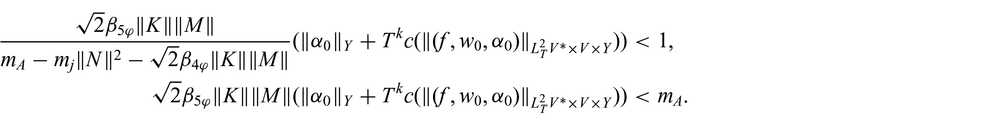
Finally, we require the following smallness-condition:
Remark 3.Similar assumptions can be found in, e.g., Shillor et al. [3], Migórski [5], Pătrulescu and Sofonea [6], Migórski and Bai [9], and Sofonea and Migórski [8]. The same type of condition as (iii) is found in, e.g., Migórski et al. [26, 27]. If is independent of and in equation (1b), we may relax the assumption (iii), and (ii) and Proposition 2 are enough.
Remark 4.If in (v), then the friction coefficient is bounded. Consequently, Problem 1 reduces to the one found in Migórski [5]. In the quasi-static setting, taking , the problem is covered in Pătrulescu and Sofonea [6]. Finally, taking reduces Problem 1 to the one found in Pipping et al. [28] and Pipping [29] for the first-order approximation of equations (64a) and (63a) introduced in Section 6.3.
We make a brief remark on the assumptions in Appendix 1.
3.2. Main result
We will now state the main result, i.e., Theorem 2; the first part is an existence and uniqueness result, and the latter provides that the flow map depends continuously on the initial data. The proof of Theorem 2 is deferred to Section 5 after the preparation in Section 4.
Theorem 2.Assume , , , , , , , , and equations (10) and (11) hold:
(a) Then, there exists asatisfying:
and
so that and is a unique solution to Problem 1.
(b) Moreover, there exists a neighborhood around so that the flow map defined by is continuous.
(c) If in (v), we obtain global time of existence, i.e., the existence of a solution holds for any finite time .
Remark 5.The theorem can easily be extended to include more than three history-dependent operators without needing any additional assumptions other than the once put on , , and , i.e., , , and , respectively.
3.3. Strategy of the proof of Theorem 2
The proof of the theorem is divided into six steps. In the first step, we introduce an auxiliary problem to Problem 1, calling this Problem 3. Specifically, we fix five of the functions in equation (8b) and leave equation (8a) intact. We recast the auxiliary problem as a differential inclusion (introduced in Section 4) and use existing results to prove that Problem 3 has a unique solution (Steps 1–4). Next, we define an iterative scheme for Problem 1 using Problem 3. This iterative scheme decouples (8a) and Problem 3 at each step. Then, we study the difference between two successive iterates and show that these iterates are Cauchy sequences. We then pass to the limit to show that the iterative scheme converges to Problem 1 (Step 5). Finally, we show that the flow map continuously depends on the initial data (Step 6).
4. Preliminary result
Before proving Theorem 2, we present an existence and uniqueness result for a differential inclusion problem (see, e.g., Aubin and Cellina [30]). The forthcoming result will be used to prove existence of a solution to an auxiliary problem of equations (8b) and (8c) in Problem 1. To utilize this result, we need to introduce a differential inclusion which we relate to the auxiliary problem of equations (8b) and (8c). This will be made clear in Steps 1 and 2 in the proof of Theorem 2.
We begin by introducing the inclusion problem.
Problem 2.Find such that:
For clarity on how to work with the preceding problem, we include the following definition.
Definition 6.A function is called a solution to Problem 2 if there exists such that:
for a.e. with:
In the preliminary existence and uniqueness result, we consider the following assumptions:
:
(i) is measurable on for all .
(ii) .
(iii) , , .
(iv) such that , .
We further assume that the operator satisfies , and the source term and the initial data satisfy equation (10a). In addition, we assume that the following smallness-condition holds:
Theorem 3.Assume that , , andequations (10a)and (13) hold. Then, Problem 2 has a unique solution in the sense of Definition 6 for any .
The theorem was proved in Migórski and Bai [9, Theorem 3]. This result will be used in Step 5 of the proof of Theorem 2.
5. Proof of Theorem 2
With the preparation in Sections 2–4, we proceed to the proof of Theorem 2. For the convenience of the reader, the proof is established in several steps, and some of the proofs have been moved to the appendix. We recall that the function spaces are defined in Section 2.2.
Step 1 (Auxiliary problem to the evolutionary hemivariational–variational inequality (8b) and (8c)). Let be given, then we define an auxiliary problem to equations (8b) and (8c) in Problem 1.
Problem 3.Find corresponding to such that:
for all , a.e.with:
Remark 6.A glance at Problem 3 andequation (8b)lets us see that the auxiliary problem keeps , (still denoted by ), , , and known in contrast toequation (8b). We find it worth mentioning that we use the subscripts on to emphasize that a solution to Problem 3 corresponds to . This also helps to distinguish between a solution to Problem 1 and a solution to Problem 3.
Step 2. (Existence of a solution to Problem 3). Let be given. We wish to utilize Theorem 3 in order to prove that Problem 3 has a solution. We therefore define the functional by:
for all , a.e. . Verification of the hypothesis of Theorem 3 follows from the same approach as the first part of the proof in Migórski and Bai [9, Theorem 5]. We investigate the assumption and the smallness-condition (13), as there are some modifications in comparison to Migórski and Bai [9. Theorem 5]. Keeping Proposition 3 in mind, we only comment on the changes and leave the reader to visit Migórski and Bai [9, Theorem 5] for a detailed verification. Using equation (9), we find that holds with , , and . This, together with the smallness-condition (11) leads to equation (13). Thus, we conclude by Theorem 3 that there exists a solution of Problem 2 with defined in equation (14). It remains to show that the existence of a solution to Problem 2 implies the existence of a solution to Problem 3. This is a consequence of Definitions 4 and 5, and basic results of the generalized gradients (see, e.g., Han and Sofonea [10, Theorem 3.7, Proposition 3.10-3.12], where they have summarized these properties, and Sofonea and Migórski [8, Lemma 7, p. 124]). A more detailed approach to this part can be found in, e.g., Han and Sofonea [10, Section 6] or Sofonea and Migórski [8, p. 190–192].
Step 3 (Uniqueness of a solution to Problem 3). Uniqueness is immediate from the proof in [8, Theorem 98] with and the smallness-condition (11), i.e., .
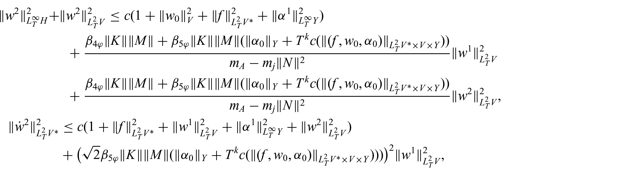
Step 4 (Estimate on the solution to Problem 3). We now find an estimate on the solution to Problem 3, which will come in handy later.
Proposition 5.Under the assumptions of Theorem 2, for given , let be a solution to Problem 3. Then, there exists a constant independent of such that:
and:
The proof of Proposition 5 is postponed to Appendix 2.
Step 5 (Scheme for the approximated solution to Problem 1). For , let , and be known. We construct the approximated solutions to Problem 1, where is a solution of the scheme:
for all , a.e. , and:
with and .
Step 5.1 (Existence and uniqueness of to equations (16a)–(16c) for all ). We establish existence and uniqueness by induction on . First, applying Minkowski’s inequality, Young’s inequality, integrating over the time interval , and finally applying the Cauchy–Schwarz inequality to hypothesis , , and , respectively, yield:
for all . We combine equations (17)–(19) with the estimates equations (15a) and (15b) in Proposition 5 for , , , , , , and . This implies:
for all . Applying Minkowski’s inequality to equation (16c) reads:
for a.e. . We observe that by Minkowski’s inequality, (ii) and :
for a.e. . Accordingly, the Cauchy–Schwarz inequality and (iii) implies:
for a.e . By Grönwall’s inequality (see, e.g., Evans [17]), we have:
and from Young’s inequality:
for . We will show the uniform bound by induction on .
From the smallness-assumption (11), it follows that:
We next define the complete metric space:
and the operator by:
for . We verify that is indeed a solution to equation (16c) for in the next lemma.
Lemma 2.Let be a solution ofequations (16a)and
(16b)
with and . Under the assumptions of Theorem 2, the operator , defined byequation (24), has a unique fixed-point, i.e., there exists a constant such that:
The proof of Lemma 2 is moved to Appendix 3 as it follows from the standard ODE arguments combined with the estimate (23), and the assumptions and . Next, investigating . This implies:
From estimate (22a) for , we have that:
for . Choosing such that:
small enough for some . From the smallness-condition (11) and the choice of , we have that:
Gathering the above and using equation (23) implies:
Moreover, verifying that is indeed a solution to equation (16c) for follows by the same approach as for .
The induction step follows the same procedure as for . Consequently, is the approximated solution of equations (16a)–(16c). Furthermore, we obtain the following uniform bound:
for all . In addition, it follows from Proposition 1 that .
Step 5.2 (Convergence of the approximated solution). We first show that is a Cauchy sequence in . This is summarized in the proposition below.
Proposition 6.Let and . Under the hypothesis of Theorem 2, let be the solution of equations (16a)–(16c). Then, is a Cauchy sequence in . In addition, , , and are the Cauchy sequences in , , and , respectively.
Remark 7.To cover the case where we obtain global time of existence when , the proof needs to be slightly modified. This case is included in Corollary 1.
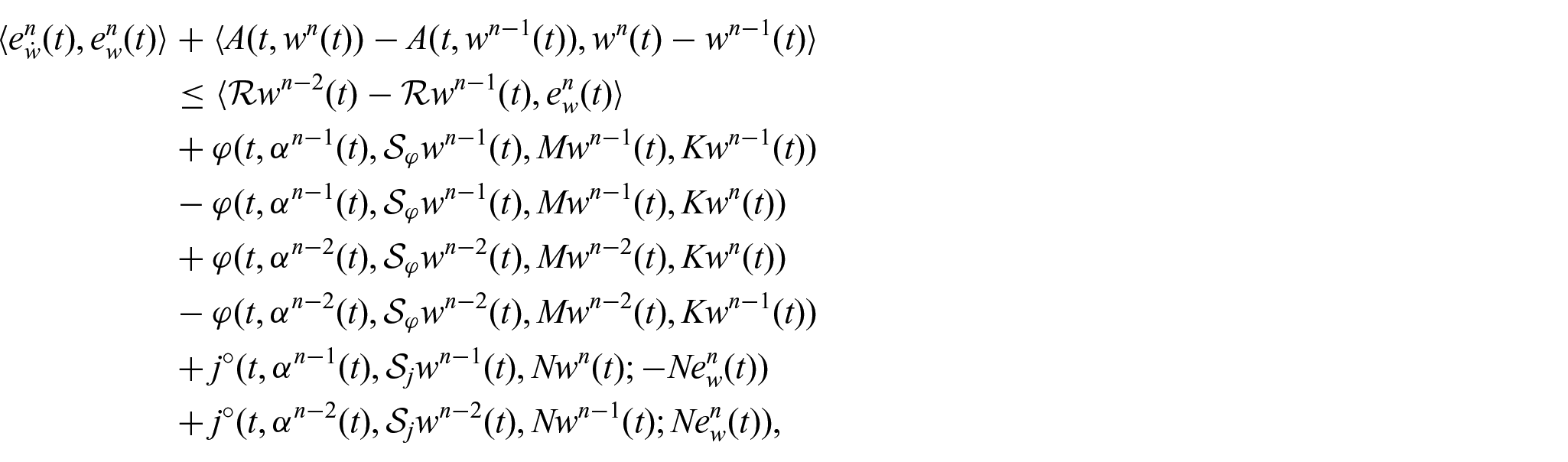
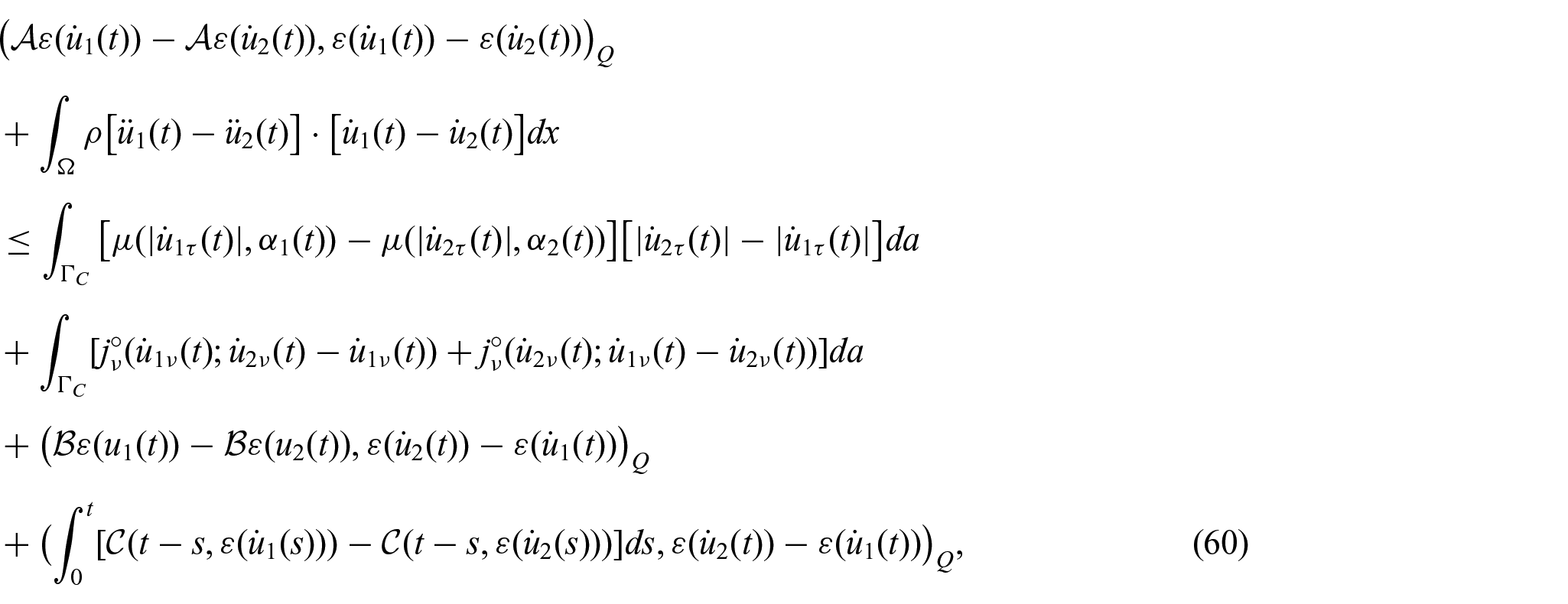
Proof. Let , , and . To begin with, we add equation (16a) for two iterations at the levels and . Then, choosing and for the levels and , respectively, implies:
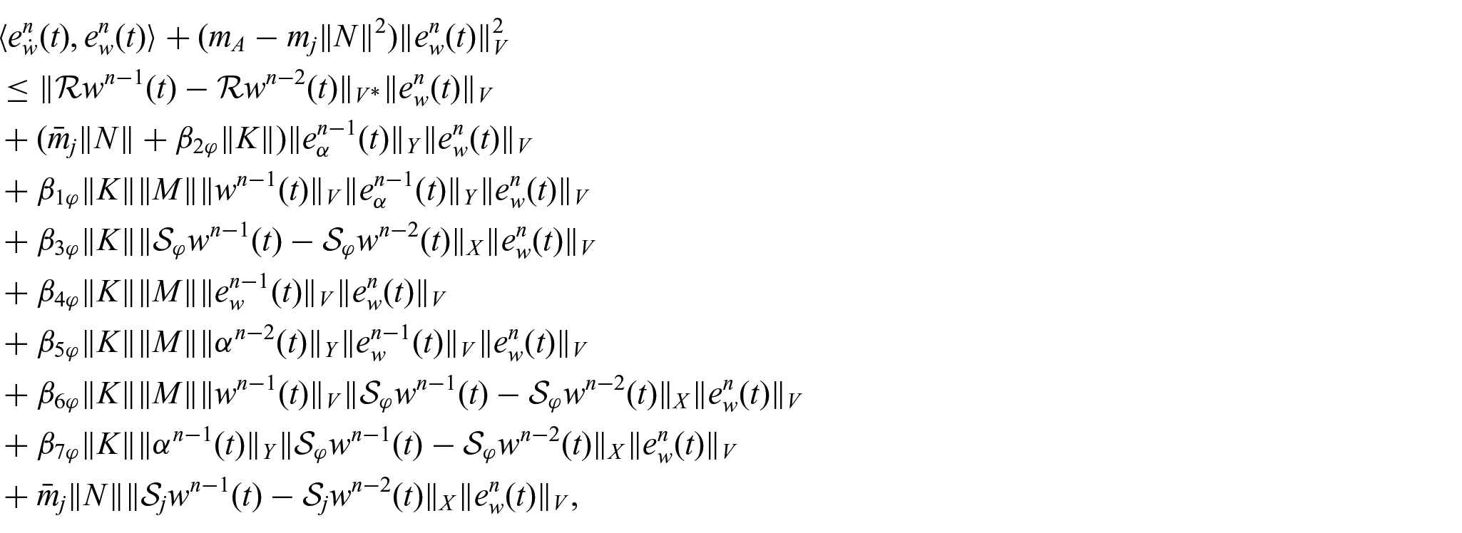
for a.e. with . We deduce from hypotheses (iv), (v), (v), , and the Cauchy–Schwarz inequality that:
for a.e. . Integrating over the time interval , we observe after using the integration by parts formula in Proposition 1 (with for a.e. ) and the Cauchy–Schwarz inequality that:
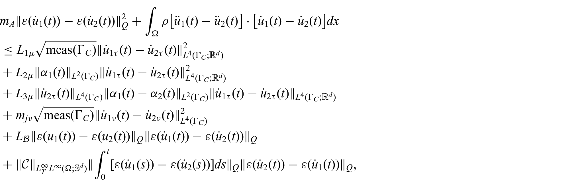
for a.e. . We may apply the Cauchy–Schwarz inequality to , , , , and . For and , we, respectively, apply Hölder’s inequality with and . To treat , we observe by the Cauchy–Schwarz inequality and (i) that:
for a.e. . Therefore, we may use Hölder’s inequality with . Similarly, by (i) and (i), respectively, we obtain:
for a.e. . In addition, using that and the smallness-assumption (11), then:
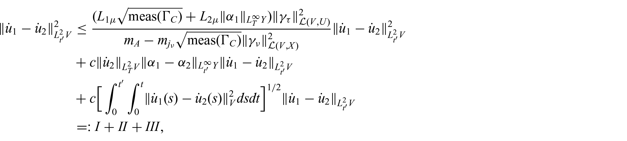
for all . Gathering the above and dividing by , we have:
for all and . Next, subtracting equation (16c) for two iterations at the levels and . Utilizing Minkowski’s inequality and (ii) yields:
for a.e. . Applying a standard Grönwall argument and the Cauchy–Schwarz inequality reads:
Applying Young’s inequality to and and then the arithmetic–quadratic mean inequality to the latter term, we obtain:
From equation (77) and Young’s inequality, the terms and become:
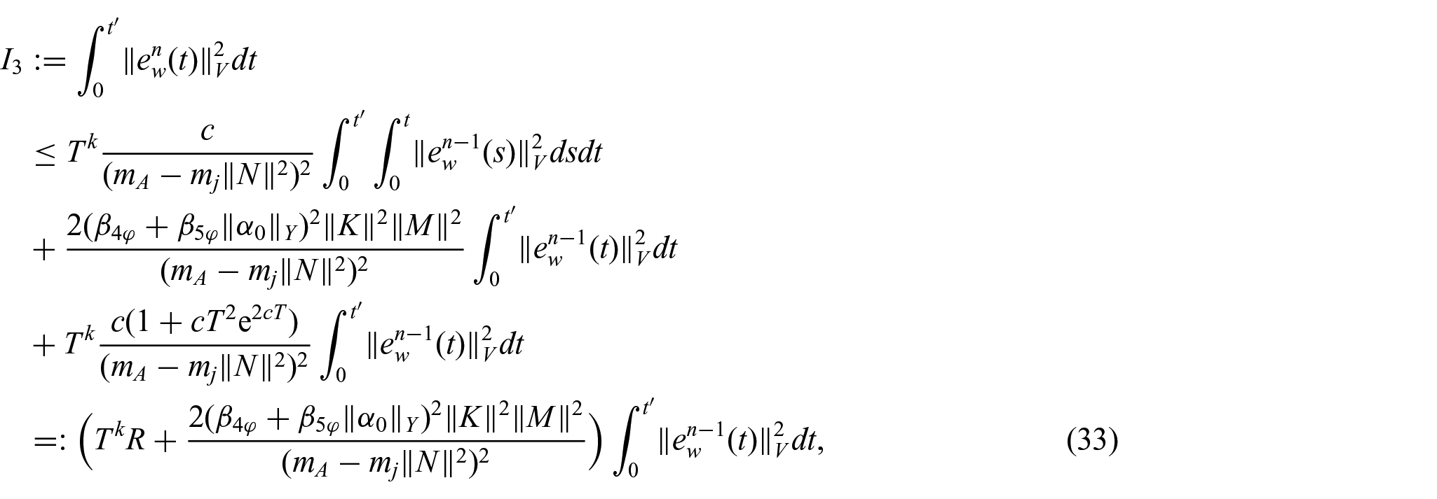
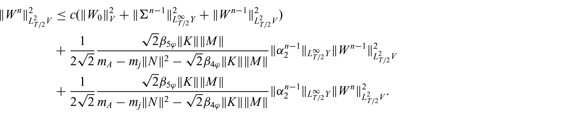
for some . Gathering the above estimates and noting that by the smallness-assumption (11) reads:
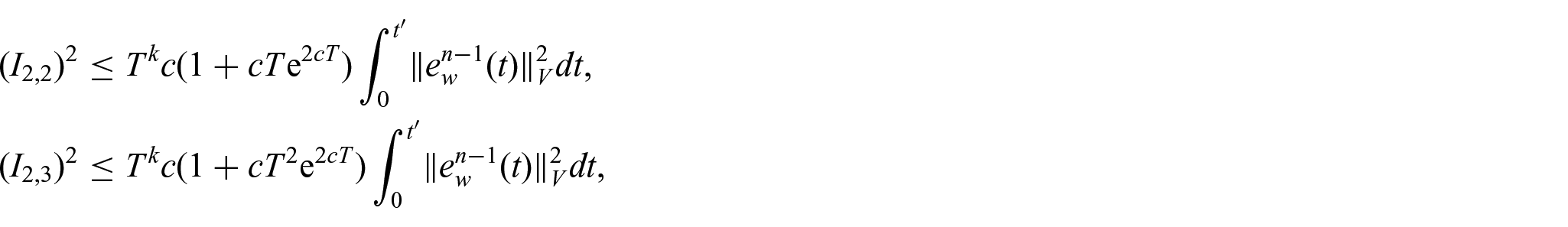
for all and some . Here,
The aim is to get the right-hand side of equation (33) to go to zero as . We will combine the smallness condition (11) and the assumption on the final time .
Iterating over , we have that:
Choosing such that:
small enough for some , the smallness-assumption (11) implies that:
Hence, equation (23) and then passing the limit gives us:
as desired.
Consequently, iterating over in equation (33), and then passing the limit gives us that is a Cauchy sequence in , and equation (77) implies that is a Cauchy sequence in . Moreover, is a Cauchy sequence in by equation (28). Similarly, is a Cauchy sequence in by equation (27), and is a Cauchy sequence in by equation (29). Concluding the proof. □
Corollary 1.Let and . Under the hypothesis of Theorem 2 with , let be the solution ofequations (16a)–(16c)for any time . Then, is a Cauchy sequence in . In addition, , , and are the Cauchy sequences in , , and , respectively.
The proof of Corollary 1 can be found in Appendix 4.
Step 5.3 (Passing the limit in equations (16a)–(16c)). From Proposition 6, it follows as that:
We are now in a position to pass the limit in equations (16a)–(16c). First, by equation (26), we have that and are uniformly bounded in and , respectively. Then, by the Eberlein–Šmulian theorem, as is a reflexive Banach space, we have, upon passing to a subsequence, that:
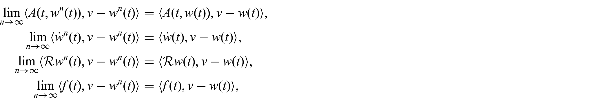
Now, with equations (35a)–(35c) in mind, we find by a proof of contradiction (assuming that the below does not hold thereby obtaining a contradiction with equations (35a)–(35c)) that:
as . By similar arguments, we find by equation (26) that for a.e. is uniformly bounded in (see, e.g., the first part of the proof of Zeng and Migorski [31, Lemma 13]). Since is a reflexive Banach space, it follows by the Eberlein-Šmulian theorem, up to a subsequence, that weakly in for a.e. . By uniqueness of limits, we have by equation (36a) that for a.e. . Following the same reasoning shows that for a.e. is uniformly bounded in . Thus, as :
for all , a.e. . Next, by equations (36a), (36e)–(36f) and (37), and the Cauchy–Schwarz inequality, we can find that:
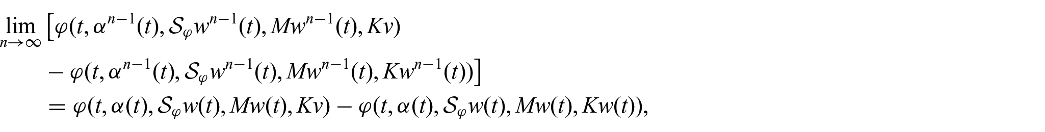
for all , a.e. . Furthermore, let be equipped with the norm . We wish to deduce that is continuous on for a.e. by applying Lemma 1. The conditions (1) and (3) are directly obtained by (ii),(iv). Finally, we find that condition (2) holds by Proposition 3. Indeed, as is lower semicontinuous and convex in its last argument, by (iii), and the fact that is finite (does not take the values ), it then follows by equations (36a)–(36c) and that:
for all , a.e. . Next, we have by (ii), that is continuous on for a.e. . From equations (21), (iii), and (26), we obtain the desired bound, i.e., integrable and independent of . Combining equations (36a), (36b), and , we may apply the dominated convergence theorem to conclude:
for all . Thus, passing the upper limit in equations (16a)–(16c) gives us that is indeed a solution to Problem 1.
Step 6 (Continuous dependence on initial data). For simplicity of notation, we define equipped with the norm . Consider two sets of initial data , we aim to prove that for all , there exists a , which will be fixed later, such that:
implies:
We consider the time interval with as in equation (12) to guarantee that . Here, are two solutions to Problem 1 corresponding to . That is, for , is the solution to:
for all , a.e. with:
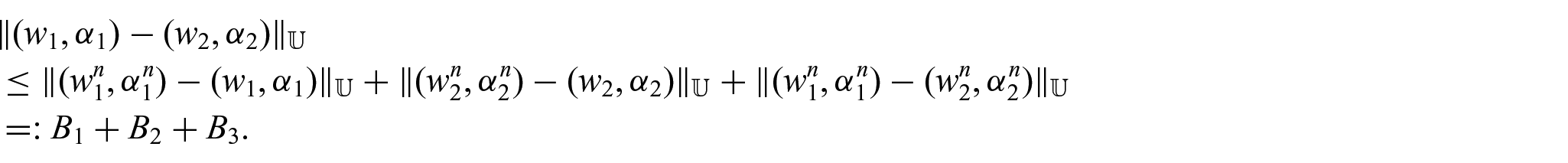
Let be the two solutions of equations (16a)–(16c) corresponding to the data for . Then, we observe that:
By Step 5.2, we have that strongly in when . Consequently, and must at least satisfy the estimate:
While for , we need the continuity of the flow map with respect to equations (16a)–(16c). We add the two inequalities and choose for a.e. and , . Let be given, and and . Then, and solves:
for a.e. with:
and
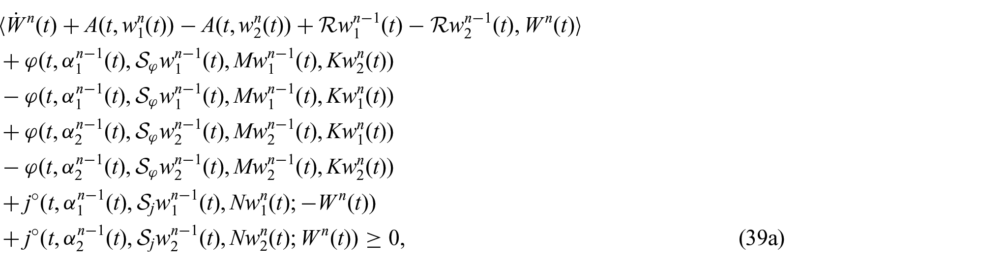
for a.e. . To find the desired estimates, we need the following lemma.
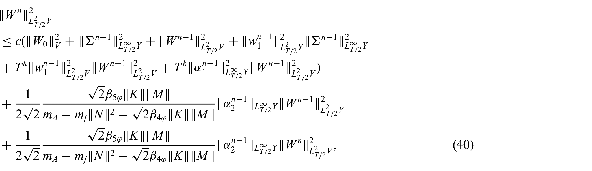
Lemma 3.Let and for . Under the assumptions of Theorem 2, let be the solution toequations (39a)–(39c). Then:
for all and some .
The proof of Lemma 3 is postponed to Appendix 5. From equations (25) and (26), and estimate (40) becomes:
In a similar manner as we obtained equation (22b), we see from equation (39c), a standard Grönwall argument, the Cauchy–Schwarz inequality, and Young’s inequality that:
By induction of , it follows the same procedure as in Step 5.1 that:
Step 7 (Proof of Theorem 2). We now have all the tools to prove the main theorem.
Proof of Theorem 2. Combining Steps 5–5 gives us well-posedness of Problem 1. □
6. Viscoelastic frictional contact problems
We will present two applications to frictional contact; the first considering contact with normal compliance and the second contact with normal damped response. Moreover, in Section 6.3, we introduce a first-order approximation of a rate-and-state friction law that is covered by our framework. Let denote the displacement, the stress tensor, and the external state variable. In addition, denotes the body forces, the surface traction, and the density (Figure 1).
A standard illustration of a sliding block.
We let the spaces , , , and be defined by equations (3)–(5) and (7), respectively. We refer to Sections 2.1 and 2.2 for further definitions of the function spaces. Furthermore, let and . Let denote the normal trace operator, and denote the tangential trace operator. It then follows by Theorem 1 that and are well-defined for . For all , we let denote the normal components on , and the tangential components on . Similarly, let , and be the normal and tangential components of the tensor on , respectively.
6.1. Dynamic frictional contact problem with normal compliance
In this section, we present a system of equations describing the evolution of a viscoelastic body in frictional contact with a foundation. Viscoelastic contact problems with normal compliance and friction are discussed in, e.g., Shillor et al. [3, Section 8.3]. The normal compliance condition is used as an approximation of the Signorini nonpenetration condition. More on this can be found in Han and Sofonea [11, Chapter 5], Kikuchi and Oden [19, Chapter 11], and Sofonea and Matei [32]. We wish to study the following problem.
Problem 4.Find the displacement and the external state variable such that:
with the initial conditions:
In the above problem, equation (41a) is a general viscoelastic constitutive law, where is a viscosity operator, an elasticity operator, and is referred to as a relaxation tensor. We note that and are the short-hand notation for and , respectively. Moreover, equation (41b) is a momentum balance equation, equation (41c) denotes the Dirichlet boundary conditions, and equation (41d) the traction applied to the surface. Equation (41e) is a contact condition, where is a prescribed function describing the penetration condition. Next, equations (41f)–(41g) denote a generalized Coulomb’s friction law, and equation (41h) describes the evolution of the external state variable (see Section 1.2 for a discussion on this equation). Finally, equations (41i) and (41j) are the initial conditions. We wish to investigate equations (41a)–(41j) under the following assumptions:
:
(i) For any is measurable on .
(ii) There exists such that for all , a.e. .
(iii) There exists such that , for all , a.e. .
(iv) for a.e. .
:
(i) For any is measurable on .
(ii) There exists such that for all , a.e. .
(iii) .
:
(i) The mapping is measurable on for all .
(ii) There exist such that for all , , a.e. .
(iii) There exist such that for all , , a.e. .
:
(i) The mapping is measurable on for all .
(ii) There exists such that for all , a.e. .
(iii) There exists such that for all , a.e. .
:
(i) The mapping is measurable on for all .
(ii) There exists such that for all , a.e. .
(iii) .
:
(i) for all , a.e. .
(ii) with .
with the initial data satisfying:
Remark 8.Similar assumptions on the operators and data are found in, e.g., Migórski [5], Pătrulescu and Sofonea [6], and Sofonea and Migórski [8]. In comparison, the assumptions (ii) and (iii) are generalized. In particular, we relaxed the boundedness assumption on .
We refer the reader to Appendix 1 for a discussion on applications under these assumptions.
6.1.1. Variational formulation
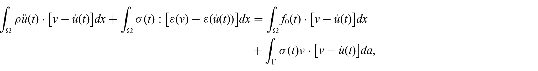
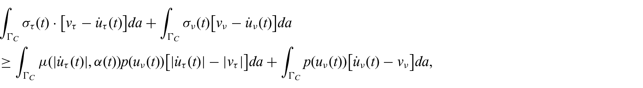
We find a formal derivation of the variational formulation of Problem 4, i.e., assuming sufficiently regular functions, as we only are interested in a mild solution (see Definition 1). We refer to, e.g., Shillor et al. [3, Section 5.2] for a more detailed derivation, especially how to deal with the contact conditions. Inserting equation (41b) into Green’s formula (6) yields:
for all , a.e. . From the terms on , we deduce:
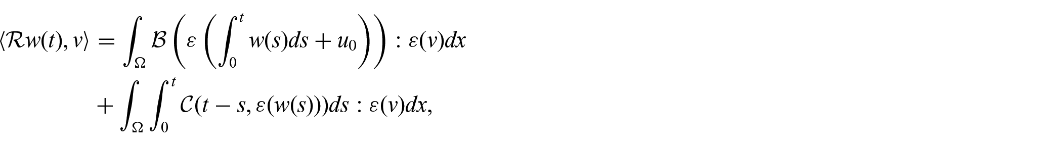
for all , a.e. . Combining the above reads:
for all , a.e. . We write the above inequality slightly more compactly. We observe that the map is linear and bounded in . Consequently, the Riesz representation theorem implies the existence of such that:
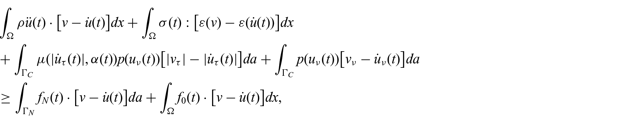
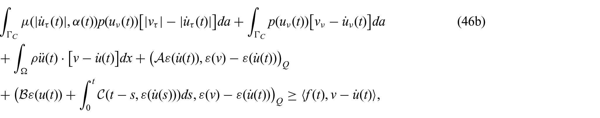
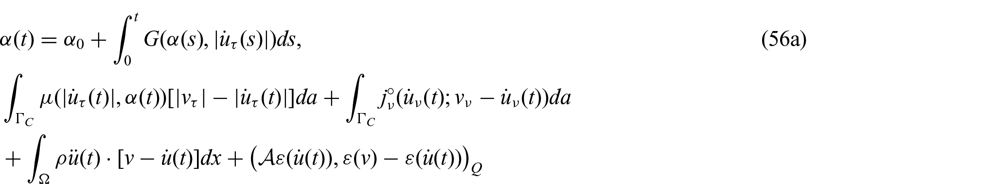
As mentioned, we are interested in a mild solution of equation (41h) (see Definition 1), so we integrate equation (41h) over the time interval and use the initial condition (41j) to obtain this equation on the desired form. We may now formulate a variational inequality of Problem 4.
Problem 5.Find and such that:
for all , a.e. with:
Remark 9.Conversely, under the assumption of sufficient regularity, showing thatequation (46a)is equivalent toequation (41h)together withequation (41j)is an application of the fundamental theorem of calculus. Moreover, choosing the test functions with inequation (46b)implies that Problem 5 is indeed equivalent to Problem 4 (see, e.g., Pipping [7, Section 2.6] or Shillor et al. [3, Section 5.2]).
The well-posedness result for Problem 5 is summarized below.
Theorem 4.Assume that, , , , , , andequations (42)–(44) hold. Then, there exists asatisfying equation (12) such that Problem 5 has at most one solutionunder the smallness-assumption:
In addition, has the following regularity:
Moreover, there exists a neighborhood aroundso that the flow mapdefined byis continuous.
Remark 10.A similar smallness-assumption (47) is used in, e.g., Pătrulescu and Sofonea [6].
Remark 11.We will show that there exists a solution for . For , we may take .
6.1.2. Proof of Theorem 4
Our aim is to use Theorem 2 to prove Theorem 4. Our first task is to rewrite Problem 5 in the same form as Problem 1. Then, we will verify the hypothesis of Theorem 2.
Let and . We then define the operators , , , , , and , respectively, by:
We define by:
which is linear and bounded in both arguments, i.e., . We consider the functional by:
for , , , , a.e. . We let be defined as in equation (76). This yields the following generalization of Problem 5.
Problem 6.Find and such that:
for all , a.e. , with.
Remark 12.Since Problem 5 is contained in Problem 6, it suffices to show well-posedness of Problem 6.
Lemma 4.Under the assumptions of Theorem 4, the hypothesis of Theorem 2 holds for equations (48a)–(48g). Here, , , , , , , , , , , and .
To maintain the flow of this paper, the proof of Lemma 4 is placed in Appendix 6. We are now ready to prove Theorem 4.
Proof of Theorem 4. The proof relies on Theorem 2 with . In light of Lemma 4, the hypotheses of Theorem 2 are fulfilled. Consequently, is a unique solution of Problem 6. Moreover, we define the function by:
for all . As a consequence of Bochner space theory, the fact that and equation (49), we have that and . Consequently, , which implies . Furthermore, we define the set:
and show that the flow map defined by is continuous. That is, we claim that for all , there exists a , chosen later, such that
implies:
To check this, let us use the continuous dependence result in Theorem 2. We observe that:
Next, by equations (49), the triangle inequality, Minkowski’s inequality, Young’s inequality, the Cauchy–Schwarz inequality, and integrating over the time interval , we have:
6.2. Dynamic frictional contact problem with normal damped response
In our second application, we consider contact with normal damped response, i.e., a wet material or some lubrication between the foundation and the reference configuration of a viscoelastic body (see, e.g., [32]). We present the problem:
Problem 7.Find the displacement and the external state variable such that:
with
We summarized equations (54a)–(54d) and (54h)–(54j) underneath Problem 4. However, equation (54e) is a general form of the contact condition for normal damped response describing the contact with a lubricated foundation [4, Section 6.3]. Equations (54f)–(54g) are a version of Coulomb’s law of dry friction, where equations (54f)–(54g) are a generalization of Sofonea and Migórski [8, Problem 68, p.268]. We investigate Problem 7 under the hypotheses of , , , , , and equations (42)–(44). In addition, we require an assumption on in equation (54e):
:
(i) is measurable on for all , and there exists such that .
(ii) is locally Lipschitz on for a.e. .
(iii) for all , a.e. with .
(iv) for all , a.e. with .
We refer the reader to Appendix 1 for a small discussion on the assumptions on the operators and functions in Problem 7.
6.2.1. Variational formulation
We make use of the derivations in Section 6.1, but include the new term for the normal stress. By definition of the Clarke subgradient (see Definition 4) and equation (54e), we have:
Integrating over , and choosing gives us:
for all , a.e. . Combining equation (55) with the calculations from Section 6.1.1, we have the following problem.
Problem 8.Find and such that:
for all, a.e.with:
The well-posedness result for Problem 8 is stated in the following theorem.
Theorem 5.Assume that , , , , , equations (42)–(44), and hold. Then, there exists a satisfying (12) so that Problem 8 has a unique solution under the smallness-condition:
In addition, we have the regularity:
Moreover, the flow map depends continuously on the initial data.
Remark 13. The constraint (57) can also be found in, e.g., Han and Sofonea [10, Theorem 4.4] for and .
Remark 14. We show that there exists a solution for , and then take .
6.2.2. Proof of Theorem 5
We use the same approach as in Section 6.1, meaning that we will use Theorem 2 to prove Theorem 5. But to use this theorem, we need to first rewrite Problem 8 into the same form as Problem 1. Then, we will verify the hypothesis of Theorem 2.
First, recall that and . Then, take and . We define , , , and as in equations (48a)–(48d) and (45), respectively. We choose and to be as in equation (48e) and . Moreover, we define the functional by:
and the functional by:
The problem is then on the following form.
Problem 9.Find such that:
for all, a.e.with.
To see that it suffices to prove existence of a solution to Problem 9 in order for Problem 8 to have a solution, we introduce the following result, which is of a similar form as found in Sofonea and Migórski [8, Lemma 8, p.126] (see also [4, Theorem 3.47]). The result will also be useful to prove uniqueness.
Corollary 2.Assume that holds. Then, the functional defined by equation (59b) has the following properties:
(i)is measurable onfor all.
(ii)is locally Lipschitz onfor a.e..
(iii) For all, we have.
Lemma 5.Under the assumptions of Theorem 5, holds for defined byequation (59a)for , , , , , and . Moreover, defined byequation (59b)satisfies for , , , and .
The proof of Lemma 5 is placed in Appendix 7. We may now prove Theorem 5.
Proof of Theorem 5. We wish to utilize Theorem 2. The hypothesis of Theorem 2 holds by equation (57), Lemmas 4 and 5, and Corollary 2(i) and (ii). With the help of Corollary 2(iii), we may conclude that there exists a solution to Problem 8. Moreover, the fact that the flow map depends continuously on the initial data follows by the same approach as in the proof of Theorem 4. To obtain uniqueness, we let be two pairs of solutions to Problem 8. Choosing the test functions and for a.e. , respectively, in equation (56b) yields:
for a.e. . Using (ii), a standard Grönwall argument, the Cauchy–Schwarz inequality, and Minkowski’s inequality in equation (56a) implies:
for a.e. ). We next utilize (iii), (ii), , (iv), (ii), equation (42), the Cauchy–Schwarz inequality, and Young’s inequality to equation (60):
for a.e. . Next, we use the fact that if , then [17, Theorem 3 in Section 5.9.2], equation (49), and integrating over the time interval . We observe by equation (57) that . In addition, we use equation (61) and then apply Hölder’s inequality and Minkowski’s inequality to obtain:
for all . Using Minkowski’s inequality, (ii), and the Cauchy–Schwarz inequality implies:
for a.e. and . From Grönwall’s inequality, we deduce:
for some . Utilizing Young’s inequality to and and then the arithmetic–quadratic mean inequality to the latter term while keeping in mind equations (57), (58), and (61), we obtain:
for all . A consequence of equation (57) and choosing such that:
small enough for some implies:
we obtain:
for all . Applying a standard Grönwall argument reads:
By the definition of , i.e., equation (49), the smallness-condition (57), and equations (61) and (62), we conclude that is the unique solution to Problem 8. □
6.3. Application to rate-and-state friction
The coupling (2) are standard in geophysical applications in earth sciences, where the experimentally derived Dieterich–Ruina laws are commonly used. We refer to Marone [33] for an overview and comparison of some commonly used laws. There have been physical issues with the standard rate law, e.g., resulting in a negative friction coefficient. This was repaired using the regularized or truncated law (see [7, Section 1.1–1.3] and references therein), which are, respectively, given by:
where . The coefficients , , , and are the system parameters (see, e.g., [33, 34], [7, Section 1.2]). Another regularization used in the literature can be found in Roubíček [35]. The most popular rate-and-state friction laws are the aging and slip laws, respectively, described by:
with being a system parameter (see, e.g., [34]). In the framework presented in this paper, we are not able to include equations (63) and (64). The main issue is that . We therefore consider a first-order Taylor approximation of around with , which is used in equations (63a) and (64a). This leads to a first-order approximation of equations (63a) and (64a).
The first-order Taylor approximation of around reads:
We will make a formal argument to justify that these are first-order approximations.
Formal augmentations of equations (66a) and (66b). For simplicity in notation, we let and . We wish to have the same order of error for the approximation of equations (63a) and (64a) as in equation (65). For equation (66a), we are considering . We directly obtain:
Next, considering equation (66b), we are interested in the approximation (65) for . We let and . Then, by the mean value theorem:
with where . So, we have:
We also note that:
where if is close to . Consequently, we have the same order of error as in equation (65) as desired. □
Remark 15.Above, we gave formal arguments that our model is a first-order expansion around the initial value . We will now investigate if our approximated model has the same qualitative behavior as the original model. Following Rice et al. [36], the key restriction on is that when the slip rate is constant, the equation has a stable solution that evolves monotonically towards a definite value of , denoted , at which . This holds true if , which is easily verified for the approximation of given byequation (66a).
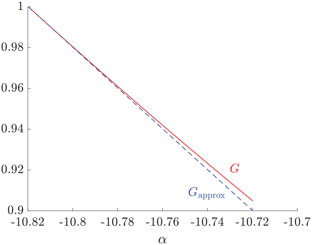
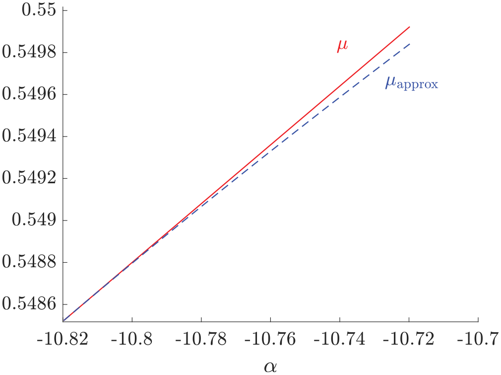
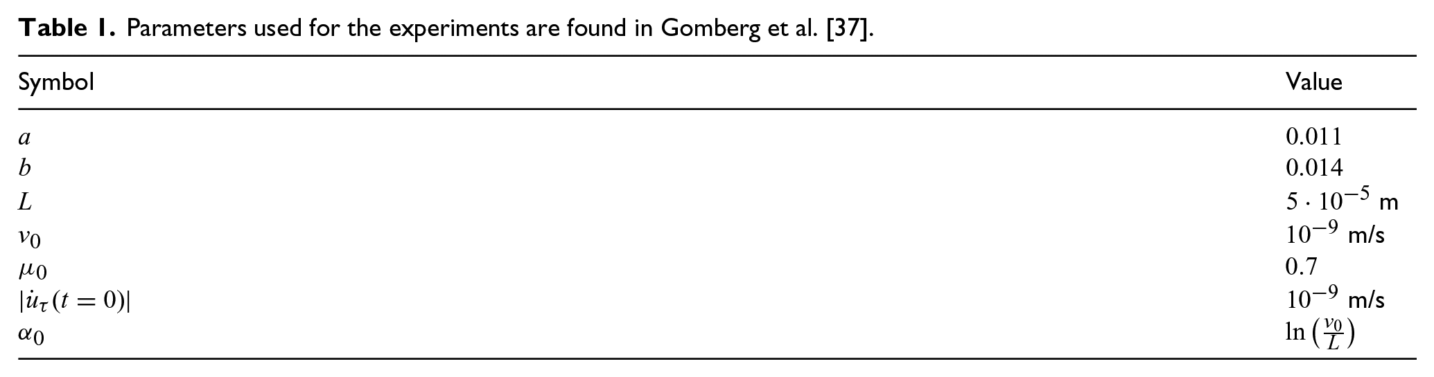
For the friction term, again following Rice et al. [36], we seek and. The first condition is consistent with the experimental observations and holds ifis close to. The latter condition agrees with the established convention for the state variable; larger values mean greater strength. This is also consistent with the usual interpretation ofas a measure of contact maturity and the fact that more mature contact is stronger. Consequently, this shows that qualitatively our approximate model has the same behavior as the original model problem. One can also see in Figures 2 and 3 that there is a neighborhood where the first-order approximations (66a) and (66b) are close to the original equations for the values used in Table 1.
With the parameters in Table 1, the red line denotes given by equation (64a), and the blue dashed line denotes , the approximation of , given by equation (66a).
The friction coefficient given by equation (63a) (red line) and , the approximated , given by equation (66b) (blue dashed line) for the parameters in Table 1.
Parameters used for the experiments are found in Gomberg et al. [37].
Symbol
Value
m
m/s
m/s
We require the following assumption on the coefficients in equations (66a) and (66b):
Then, we have the following consequences of Theorems 4 and 5, respectively.
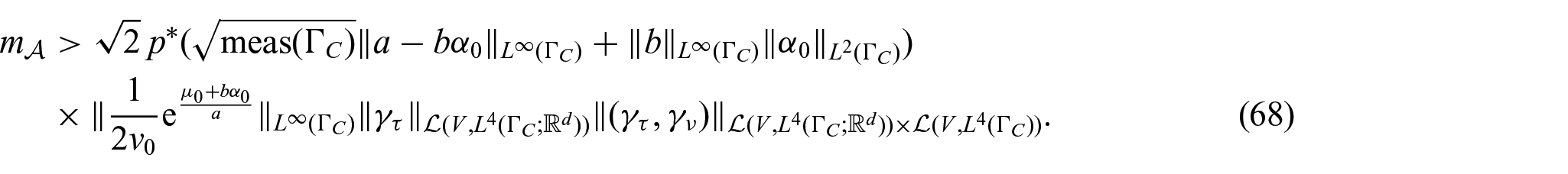
Corollary 3.Assume that hypotheses , , , , equations(42)–(44a), and (67) hold. Then, there exists a satisfying equation (12) such that Problem 5 withequations (66a)and (66b) has a unique solution under the smallness-conditions:
We obtain the following regularity:
Moreover, there exists a neighborhood aroundso that the flow map, is continuous.
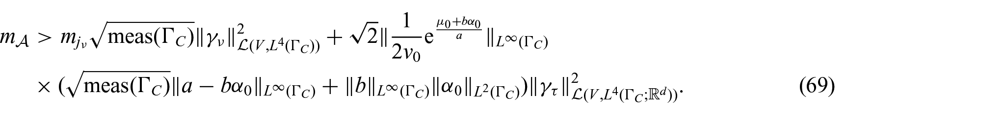
Corollary 4.Assume that , , , , , equations(42)–(44a), , and (67) hold. Then, there exists a satisfying equation (12) so that Problem 8 with equations (66a) and (66b) has a unique solution under the smallness-condition:
In addition, we have the regularity:
Moreover, the flow map depends continuously on the initial data.
Remark 16.A practical fix to get a global well-posedness result would be through a truncation operator defined by:
Then, if we replacewith, we would have that and obtain the global well-posedness by Theorem 2(c) (see also Remark 4 on this point).
is small enough, or we must compensate by adding more viscosity.
Remark 18.In Pipping et al. [28] and Pipping [29], they study equations (63) and (64) in a time-discrete setting with (the normal stresses are constant—referred to as Tresca friction), being independent of in its third argument, relaxing the structure of (see Remark 4), and putting in Problem 1.
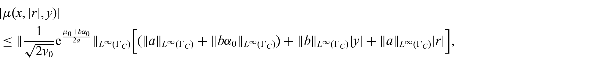
Proof of Corollary 3. We only need to verify and for equations (66a) and (66b), respectively. The rest follows by Theorem 4 since . We start by verifying for equation (66a). From equation (67), we directly have that (ii) and (iii) hold with Next, we verify for equation (66b).
which is (iii) for , , and . Finally, to verify (ii), we use equation (70b) and the triangle inequality:
Thus, (ii) holds with and . We finally observe that the smallness-condition (47) holds by equation (68).
Proof of Claim 1. Since is symmetric for , we may prove equation (70a) for . By the mean-value theorem, it follows that:
By definition , then by the fact that and the increasing property of the logarithm, we have:
Then, from equation (71), we conclude that equation (70a) holds. Similarly, without loss of generality, we may assume that , then by the mean-value theorem:
Proof of Corollary 4. The proof follows by Theorem 5 and the verification of and for equations (66a) and (66b), which is done in the proof of Corollary 3. In addition, the smallness-condition (57) holds by equation (69). □
Footnotes
Appendix 1
Appendix 2
Proof of Proposition 5. For the simplicity of notation, let . We start off finding estimates on , , and . According to (iv):
for a.e. . Invoking (iii), i.e., , and the Cauchy–Schwarz inequality gives:
for a.e. . Next, we take a closer look at . Keeping in mind Definition 4 and applying (iv) and (v) and the Cauchy–Schwarz inequality reads:
for all , a.e. . Similarly, we observe by Definition 5, (iv) and (v), and the Cauchy–Schwarz inequality that:
for all , a.e. . We are now in a position to find the desired estimate. Choosing in Problem 3, while keeping in mind , reads:
for a.e. . Take in equations (75) and (76) and combine with equation (74). Next, we integrate over the time interval and apply the Cauchy–Schwarz inequality to equation (75), , , , and . We apply Hölder’s inequality with to . Applying the integration by parts formula in Proposition 1 (with for a.e. ) yields:
for a.e. . Next, using the fact that , that is a continuous embedding, and applying Young’s inequality implies that there exists such that:
for a.e. . Now, we choose which implies that from equation (11).
It remains to find equation (15b). Let us first rearrange Problem 3. Then, the estimates (75) and (76) and the Cauchy–Schwarz inequality implies:
for all , a.e. . Next, choosing with arbitrary. By duality, we deduce:
for a.e. . We square both sides and apply the arithmetic-quadratic mean inequality first to and , and then to the latter term implies:
We obtain the desired inequality integrating over the time interval and utilizing Hölder’s inequality.
Appendix 3
Proof of Lemma 2. The proof relies on the Banach fixed-point theorem. We, therefore, need to verify that the map is indeed well-defined and that it is a contractive mapping on . For the sake of presentation, we split the proof into two steps.
Step i (The operator is well-defined on ). Indeed, . We first prove that for given , then . We apply Minkowski’s inequality to equation (24), then we utilize estimate (21) with and together with and (iii). This yields:
for a.e. . From Hölder’s inequality and the Cauchy–Schwarz inequality, we obtain:
We then see from Young’s inequality and estimate (34) that:
Choosing such that it provides the desired upper bound concludes this part.
It remains to show that is continuous in for a.e. for given and . Let , then with no loss of generality, we assume that . We then use Minkowski’s inequality, estimate (21) (with and ), Hölder’s inequality, the Cauchy–Schwarz inequality, , and (iii) to deduce:
Estimate (23) implies:
for . Passing the limit , we have that indeed .
Step ii (The application is a contractive mapping). Let , , and let be a unique solution to equations (16a)–(16c). We introduce a new norm in :
where is chosen later. We notice that with is complete and is equivalent to the norm on . Then, from equation (24), we have:
Choosing implies that is a contraction on , and thus, we may conclude by the Banach fixed-point theorem that is a unique fixed point to equation (24). □
for all and some . From a standard Grönwall argument (see, e.g., [32, Lemma 3.2]) combined with Young’s inequality, and the Cauchy–Schwarz inequality applied to equation (31), we obtain:
for a.e. and some . Applying Young’s inequality and equation (77), we have:
Iterating over implies:
We observe that:
Now, since and:
we have:
We may therefore conclude the proof in the same way as in the proof of Proposition 6. □
Appendix 5
Proof of Lemma 3. For equation (39a), we utilize the conditions (iv), (v), (v), and the Cauchy–Schwarz inequality to obtain:
for a.e. . First, integrating over the time interval , applying the integration by parts formula in Proposition 1 (with for a.e. ), Young’s inequality, Hölder’s inequality, , and the fact that is a continuous embedding. Second, we apply the Cauchy–Schwarz inequality to , , and , respectively, gives us the following estimates:
for a.e. . This yields:
for . Keeping in mind equation (11), we may choose to obtain the desired result. □
Appendix 6
Proof of Lemma 4. The assumptions on , , hold directly by the hypothesis with , , and (see, e.g., [8, p.273]). Second, holds by with and is history-dependent with by and (ii) (see, e.g., [8, p.275]). We observe that (ii) holds by a duality argument, the Cauchy–Schwarz inequality, (ii), and equation (44a). Moreover, it follows directly by Minkowski’s inequality and the properties of the trace operator that (i) and (ii) hold with . In addition, equations (10) and (11) are a consequence of equations (43) and (44) and a duality argument.
The verification of requires some work. First, (i) holds as the variables in equation (48g) do not explicitly depend on . Next, we show that is continuous on for all , a.e. . That is, ensuring that (ii) holds. Let such that . Then:
For simplicity in notation, we let:
then
We estimate directly by Hölder’s inequality and (ii), while for and , we use Hölder’s inequality, (iii), and (ii). This reads:
To verify (iii), we first note that a continuous function is lower semicontinuous. So, it suffices to show that is Lipschitz continuous on for all , , , a.e. . Let , , then (ii)-(iii), (iii), and Hölder’s inequality yield:
for all , , , a.e. . The triangle inequality and the linearity of the integral guarantee the convexity in the last argument of . Thus, we have that (iii) holds.
From equation (78) and , we observe that (iv) holds for , , , , and . We finally verify (v). Let , , , , for . Then:
For simplicity, we define:
then by (iii), (ii), and the triangle inequality:
Next, we apply Hölder’s inequality and (iii) to obtain:
Hence, (v) holds with , ,
, , , , and . □
Appendix 7
Proof of Lemma 5. We will first prove that defined by equation (59a) satisfies . First, (i) holds as the variables in equation (59a) do not explicitly depend on . Next, (ii) holds, i.e., is continuous on for all , a.e. . Indeed, let such that , it then follows by (ii) and Hölder’s inequality that:
for all . Moreover, convexity in the last argument of follows by the triangle inequality and the linearity of the integral. In addition, a continuous function is lower semicontinuous. Therefore, we will show that is continuous in its last argument. Let such that . Then, the Cauchy–Schwarz inequality and (iii) give:
for , , , , a.e. . This proves (iii). Similarly as in the proof of Lemma 4, equation (79) implies that (iv) holds for , , , and . Finally, we investigate (v). From hypothesis (ii) and Hölder’s inequality, we obtain:
for all , , for , a.e. We set , , , and . Finally, we prove that defined by equation (59b) satisfies . Corollary 2(i) and (ii) guarantees that (i) and (ii). It remain to show that (iii)-(v). From Corollary 2(iii), Proposition 2, and Fatou’s lemma, we obtain (iii). We find that (iv) holds by (iii), Young’s inequality, and Hölder’s inequality. Indeed,
implies:
with , , and . For (v), we use Corollary 2(iii) (see, e.g., [5]), (iv), and the Cauchy–Schwarz inequality to obtain:
where , concluding this proof.
Acknowledgements
N.S.T. thanks Meir Shillor for many important comments that improved a previous version of this manuscript. We also thank the anonymous referees for their careful reading and helpful comments.
Funding
This research was supported by the VISTA program, The Norwegian Academy of Science and Letters, and Equinor.
ORCID iD
Nadia Skoglund Taki
References
1.
DancerENDuY. On a free boundary problem arising from population biology. Indiana Univ Math J2003; 52: 51–67.
2.
DuvautGLionsJL. Inequalities in mechanics and physics. Berlin: Springer-Verlag, 1976.
3.
ShillorMSofoneaMTelegaJJ. Models and analysis of quasistatic contact: variational methods. Berlin: Springer, 2004.
4.
MigórskiSOchalASofoneaM. Nonlinear inclusions and hemivariational inequalities: models and analysis of contact problems. New York: Springer, 2013.
5.
MigórskiS. Well-posedness of constrained evolutionary differential variational-hemivariational inequalities with applications. Nonlinear Anal Real World Appl2022; 67: 103593.
6.
PătrulescuFSofoneaM. Analysis of a rate-and-state friction problem with viscoelastic materials. Electron J Diff Equ2017; 299: 1–17.
7.
PippingE. Dynamic problems of rate-and-state friction in viscoelasticity. PhD Thesis, Freie UniversitätBerlin, Berlin, 2014.
MigórskiSBaiY. Well-posedness of history-dependent evolution inclusions with applications. Z Angew Math Phys2019; 70: 144.
10.
HanWSofoneaM. Numerical analysis of hemivariational inequalities in contact mechanics. Acta Numer2019; 28: 175–286.
11.
HanWSofoneaM. Quasistatic contact problems in viscoelasticity and viscoplasticity. Providence, RI: International Press; Sommerville, MA: American Mathematical Society, 2002.
12.
OdenJTMartinsJAC. Models and computational methods for dynamic friction phenomena. Comput Methods Appl Mech Eng1985; 52: 527–634.
13.
ZmitrowiczA. Contact stresses: a short survey of models and methods of computations. Acta Appl Mech2009; 80: 1407–1428.
MigórskiSBaiYZengS. A new class of history-dependent quasi variational–hemivariational inequalities with constraint. Comput Math Appl2022; 114: 106686.
27.
MigórskiSCaiDDudekS. Differential variational–hemivariational inequalities with application to contact mechanics. Nonlinear Anal Real World Appl2023; 71: 103816.
28.
PippingESanderOKornhuberR. Variational formulation of rate- and state-dependent friction problems. Z Angew Math Mech2015; 95: 377–395.
29.
PippingE. Existence of long-time solutions to dynamic problems of viscoelasticity with rate-and-state friction. Z Angew Math Mech2019; 99: e201800263.
30.
AubinJPCellinaA. Differential inclusions: set-valued maps and viability theory (lecture notes in mathematics). Berlin: Springer-Verlag, 1984.
31.
ZengBMigórskiS. Evolutionary subgradient inclusions with nonlinear weakly continuous operators and applications. Comput Math Appl2018; 75: 89–104.
32.
SofoneaMMateiA. Mathematical models in contact mechanics. Cambridge: Cambridge University Press, 2012.
33.
MaroneC. Laboratory-derived friction laws and their application to seismic faulting. Annu Rev Earth Planet Sci1998; 26: 643–696.
34.
HelmstetterAShawBE. Afterslip and aftershocks in the rate-and-state friction law. J Geophys Res Solid Earth2009; 114.
35.
RoubičekT. A note about the rate-and-state-dependent friction model in a thermodynamic framework of the Biot-type equation. Geophys J Int2014; 199: 286–295.
36.
RiceJRLapustaNRanjithK. Rate and state dependent friction and the stability of sliding between elastically deformable solids. J Mech Phys Solids2001; 49(9): 1865–1898.
37.
GombergJBeelerNBlanpiedM. On rate-state and coulomb failure models. J Geophys Res2000; 105: 7857–7871.
38.
BarboteuMBartoszKHanWJaniczkoT. Numerical analysis of a hyperbolic hemivariational inequality arising in dynamic contact. SIAM J Numer Anal2015; 53: 527–550.