
Abstract
We propose a coupled electrical and mechanical bidomain model for the myocardium tissue. The structure that we investigate possesses an elastic matrix with embedded cardiac myocytes. We are able to apply the asymptotic homogenization technique by exploiting the length scale separation that exists between the microscale where we see the individual myocytes and the overall size of the heart muscle. We derive the macroscale model which describes the electrical conductivity and elastic deformation of the myocardium driven by the existence of a Lorentz body force. The model comprises balance equations for the current densities and for the stresses, with the novel coefficients accounting for the difference in the electric potentials and elastic properties at different points in the microstructure. The novel coefficients of the model are to be computed by solving the periodic cell differential problems arising from application of the asymptotic homogenization technique. By combining both the mechanical and electrical behaviors, we obtain a macroscale model that highlights how the elastic deformation of the heart tissue is influenced and driven by the difference in the electric potentials at various points in the material.
1. Introduction
The heart is a muscular organ that pumps blood around the body. The muscular walls (myocardium) of the heart are formed from individual cardiac muscle cells which are connected together to form what is known as a functional electrical syncytium. This means there are strong electrical and mechanical connections between adjacent cardiac muscle cells in every direction allowing the myocardium to behave as a single contractile unit [1]. The cardiac muscle cells are known as myocytes and are connected at each end by the gap junctions at the intercalated disks. The heart contracts to pump blood around the body because of the electrical activation of the myocytes. In order to understand the physiology and electrical activity of the heart more thoroughly, we direct the reader to Katz [2], Opie [3], and Weidmann [4].
Many approaches have been made to model the electrophysiology and mechanical behavior of the heart [5–7]. One of the most important and prominent approaches is the constitutive nonlinear elastic modeling using the Holzapfel–Ogden law [8]. Holzapfel and Ogden [8] described the myocardium as a non-homogeneous, anisotropic, nonlinear elastic, and incompressible material. They then propose a strain energy function to describe the material. The parameters of the law are determined by biological measurements. This work has been subject to a variety of extensions that aim at understanding the behavior of the heart, such as in Wang et al. [9], and numerically in Pezzuto et al. [10].
Another very important approach is to consider an electrical bidomain model. This approach considers the propagation of cardiac action potentials and was first proposed in Barr and Jakobsson [11], Eisenberg [12], and Miller and Geselowitz [13]. The model is used to describe the development of the electrical potential through the heart muscle. The model accounts for the fact that at the microscopic scale, the action potentials arise due to the flow of specific types of ions through ion channels covering the cell membrane. We should note that the bidomain modeling approach is not exclusively considered for cardiac electrophysiology and can indeed be applied to the electrophysiology of neurons, e.g., Ellingsrud et al. [14] and Schreiner and Mardal [15].
Traditionally, the bidomain model was proposed for the electrical conductivity; however, there has been the development of the mechanical bidomain model to describe the elastic behavior of the heart, see Roth [16–19]. The mechanical bidomain model is able to account for the forces acting across the cell membrane which arise from the differences in the elastic displacement of the intracellular (inside the myocyte) and extracellular domains.
Each of the different bidomain models focuses on only either the mechanical or the electrical behavior and each has different advantages. The electrical bidomain model is used to simulate the electrical stimulation of the heart to understand how a voltage develops across the membrane between intracellular and extracellular domains. This is particularly useful to investigate cardiac pacing or defibrillation [20]. On the contrary, the mechanical bidomain model is used when considering mechanical forces are acting on and across the membrane, such as in the case of heart diseases and aging.
The heart has many structural features which are generally found at different microstructural levels (or scales). We are considering the heart muscle where we wish to look at the interactions between the myocytes and the extracellular matrix. Due to this, it is appropriate to consider a scale where we can see the myocytes and matrix clearly resolved. We call this scale the microscale. This is a fine microstructural level and has an associated length which is much smaller than the one characterising the whole heart. The complete heart muscle, however, can be described by a scale which we denote the macroscale.
The heart comprises multiple scales so we wish to create a model for it that can correctly characterize the effective properties but is also computationally feasible. To meet this goal, we require to relate the macroscale governing equations to the properties and interactions of the microscale. We approach this by creating a problem that describes the behavior and interactions of all constituents on the microscale. Once you have a problem of this type, it can be used in an upscaling process to obtain macroscale governing equations. There are a variety of techniques proposed in the literature that can be used for upscaling, and these are collectively known as homogenization techniques. Techniques such as mixture theory, effective medium theory, volume averaging, and asymptotic homogenization come under this category. Each technique has a variety of benefits and choice of method should be made depending on the application of the model and the information you wish to be encoded or available from the macroscale model. Each of the above-mentioned techniques has been reviewed and discussed in Hori and Nemat-Nasser [21, 22], while, e.g., Taffetani [23] provides an overview in context of mechanobiology.
Here, we make use of the asymptotic homogenization technique. Previously, this has been popularly used in modeling poroelasticity [24, 25], elastic composites [26, 27], and electroactive materials [28–30]. The technique has also proved useful in extending the theory such as to include growth and remodeling and vascularization of poroelastic materials [31, 32]. Recently, the technique was used in the derivation of the models of poroelastic composites and double poroelastic materials [33, 34]. To illustrate that the technique produces computationally feasible results, a micromechanical analysis of the effective stiffness of poroelastic composites has been investigated in Miller and Penta [35]. The technique has also previously been used in the context of heart modeling. In Miller and Penta [36], it has been used to investigate the structural changes involved in myocardial infarction and has even been used in the context of the electrical bidomain model (see Bader et al. [1] and Richardson and Chapman [37]).
This work involves applying the asymptotic homogenization technique to the problem that we have setup to describe the electrical and mechanical interactions between the cardiac myocytes and the surrounding matrix. We consider the heart muscle at a scale where the myocytes are distinct from the matrix. This scale is our microscale. The microscale has an associated length which is much smaller than the one of the entire heart muscle (where we cannot see individual myocytes) and so the scale of the heart is known as the macroscale. We then apply the asymptotic homogenization technique to upscale the problem, accounting for the continuity of current densities, stresses and elastic displacements as well as the difference in the electric potentials across the interface between the myocyte and the matrix. The novel macroscale model that is derived is a first attempt at an asymptotic homogenization model for a coupled electrical and mechanical bidomain model. The novel model comprises balance equations for the current densities and for the stresses as well as additional terms accounting for the difference in the electric potentials at different points in the microstructure. The coefficients of the model encode the properties of the microstructure and are computed by solving the microscale differential problems arising as a result of applying the asymptotic homogenization technique.
We have organized this work as follows. Section 2 focuses on introducing the mechanical and electrical problem that describes the microscale of the heart that we are considering. This problem describes the interactions between the intracellular domain (myocyte) and the extracellular domain (matrix). Then, in section 3, we perform the multiscale analysis of the problem. This procedure allows us to derive the new macroscale model governing the homogenized mechanical and electrical behavior of the heart tissue. In section 4, we present the new macroscale model and discuss the novel terms arising from considering both mechanical and electrical bidomain models coupled together. Then, in section 5, we consider the limit case where there is no change in electric potential at the interfaces between phases and reduce the model. We also provide a scheme that could be followed to solve the model numerically. In section 6, we summarize and draw conclusions to our work and provide further perspectives.
2. Electrical and mechanical problem
We begin by considering the microstructure of the myocardium which we call a set
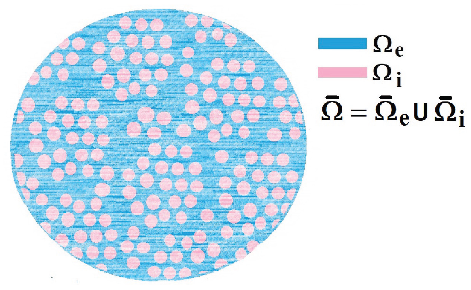
A 2D sketch representing a cross-section of the three-dimensional myocardium which we call our domain
We can then zoom in around one individual myocyte, and we see the clear microstructure which we have shown in Figure 2.
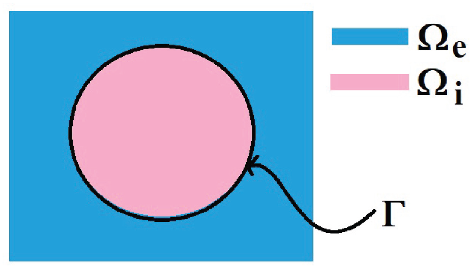
A 2D sketch representing a cross-section of the three-dimensional domain
We now wish to describe the equations that govern each domain and the chosen interface conditions to close the problem. We begin with the steady-state electrical bidomain equations:


where


which are Ohm’s law with the conductivity tensors
In order to close the electrical part of the problem, we prescribe the following conditions on the interface


where
There are also the mechanical equations for each phase. We have the balance equations given by:


where

The choice of these body forces is for a variety of reasons. The first being there has been previous use of this force in Puwal and Roth [17] where they examine a mechanical bidomain model and the effect of magnetic forces on action currents associated with a propagating action potential wavefront. By considering the same force, this will allow for future comparison with the numerical results obtained within Puwal and Roth [17]. There are also important applications such as the imaging of the elastic displacement due to Lorentz force which has been recently proposed as a potential use of MRI (see conclusions in section 6 for further discussion on this application). For further details of electroelastic materials and applied electric body forces, see, e.g., Dorfmann and Ogden [38, 39] and Maugin [40]. We should also note that the intracellular and extracellular domains are not separate from each other and interact through a variety of transmembrane proteins. This means that any displacement in the intracellular domain will cause displacements in the extracellular domain and vice versa. To cope with this, we follow the approach taken by Roth [16–18] where these interactions are described using Hooke’s law for the displacement difference and so


where


and therefore also left minor symmetries follow by combining equations (7a) and (7b). In particular, by applying right minor symmetries, we can equivalently rewrite the stress equations (6a) and (6b) as:


where

is the symmetric part of the gradient operator.
Finally, we need to close the problem by prescribing conditions on the interface


where again
3. Multiscale analysis
We now perform a multiscale analysis of the problem introduced in the previous section, which is summarized below:


The problem (11a)–(11l) is closed by prescribing suitable external boundary conditions on
3.1. Non-dimensionalization of the problem
We wish to formulate our model in non-dimensional form so as to clarify the mutual weight of each of the relevant fields in the problem. The intention is that the derived model will be general in regard to the heart microstructure so as to allow specification at a later stage to certain conditions or diseases. For this reason, we do not motivate the non-dimensionalization via specific parameters but instead perform a formal non-dimensionalization that will highlight the proper asymptotic behavior of each of the relevant fields. We make the choice to scale the spatial variable and the elastic displacement, and therefore the stresses and elasticity tensors, by the characteristic length scale L of the domain and an elastic scaling parameter E,
We are then able to use equation (12) and observe that:

These are substituted into equations (11a)–(11l) to obtain the following non-dimensional form of the system of PDEs:


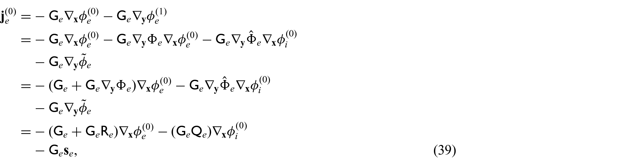
where

are the dimensionless parameters.
In the next section, we introduce the asymptotic homogenization technique which is used to upscale the non-dimensional system of PDEs (14a)–(14l) by formally assuming that the microscale and the macroscale are well separated.
3.2. The asymptotic homogenization technique
In this section, we introduce the two-scale asymptotic homogenization technique which is used to derive a macroscale model for equations (14a)–(14l). We first assume that the microscale (where individual myocytes are clearly resolved from the matrix), denoted by

We then introduce a local spatial variable to capture microscale variations of the field via setting:

The spatial variables

We further assume that all the fields

where

i.e., it depends only on the macroscale at order zero. This assumption has also been made in Richardson and Chapman [37].
We make the following two assumptions in the next sections of this work.

where
3.3. Multiple scales expansion
We apply the asymptotic homogenization assumptions (18) and (19) to equations (14a)–(14l) to obtain, accounting for periodicity, the following multiscale system of PDEs:


We can now substitute power series of the type

where the integral average can be performed over one representative cell due to
Equating coefficients of


From equations (24i) and (24j), we see that


Since we have the interface condition (24l)

throughout the following sections.
Due to the assumption (20) that

We then write the


The boundary value problem (28a)–(28d) is a linear-elastic type problem with no source terms in equations (28a) and (28b). It is equipped with the jump condition (28d) between the current densities and with the continuity condition between the zero-order electric potentials (28c). For problems of the type (28a)–(28d), it has been proved that the only solutions are constant with respect to the macroscale variable


This means that balance equations (24g) and (24h) can be rewritten as:


Similarly, we can now equate the coefficients of


Now that we have equated the coefficients of powers 0 and 1 of
3.4. Problem for electric potentials
and
Using equations (31a)–(31c) and (31f), we can form the following problem for the electric potentials


Exploiting the linearity of problem (32a)–(32d), we can propose the following ansatz:


where


and


and


where periodic conditions also apply on the boundary

Since we now have expressions for
and
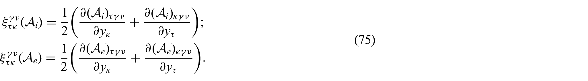
where we have used the notation:

We now require a balance equation for the current densities. This requires us to equate the powers of


with the


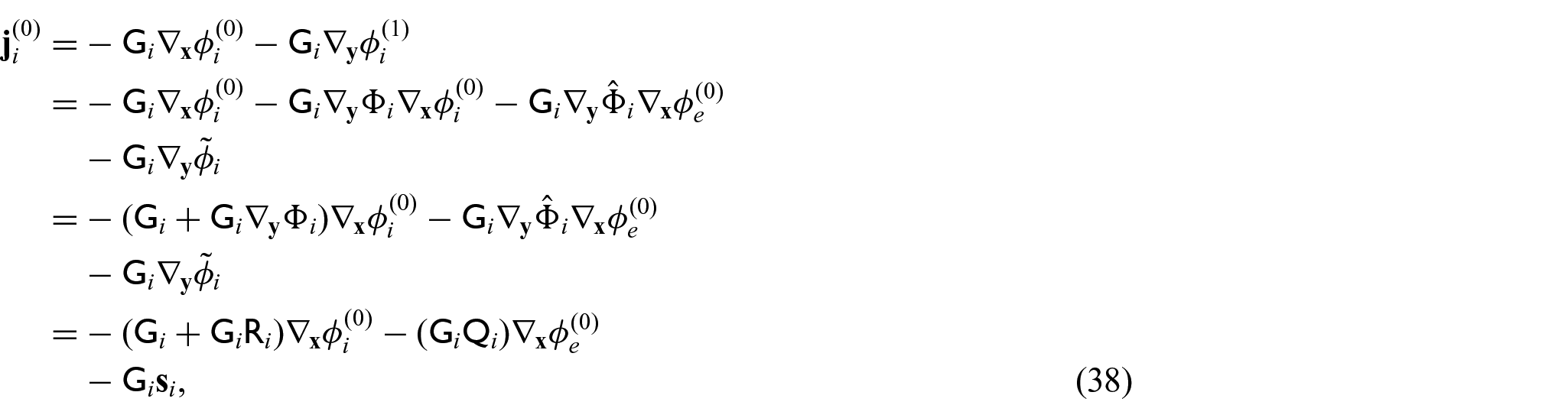
We can then use equations (42a) and (42b), along with equations (31d) and (31e) in equations (41a) and (41b) to obtain:


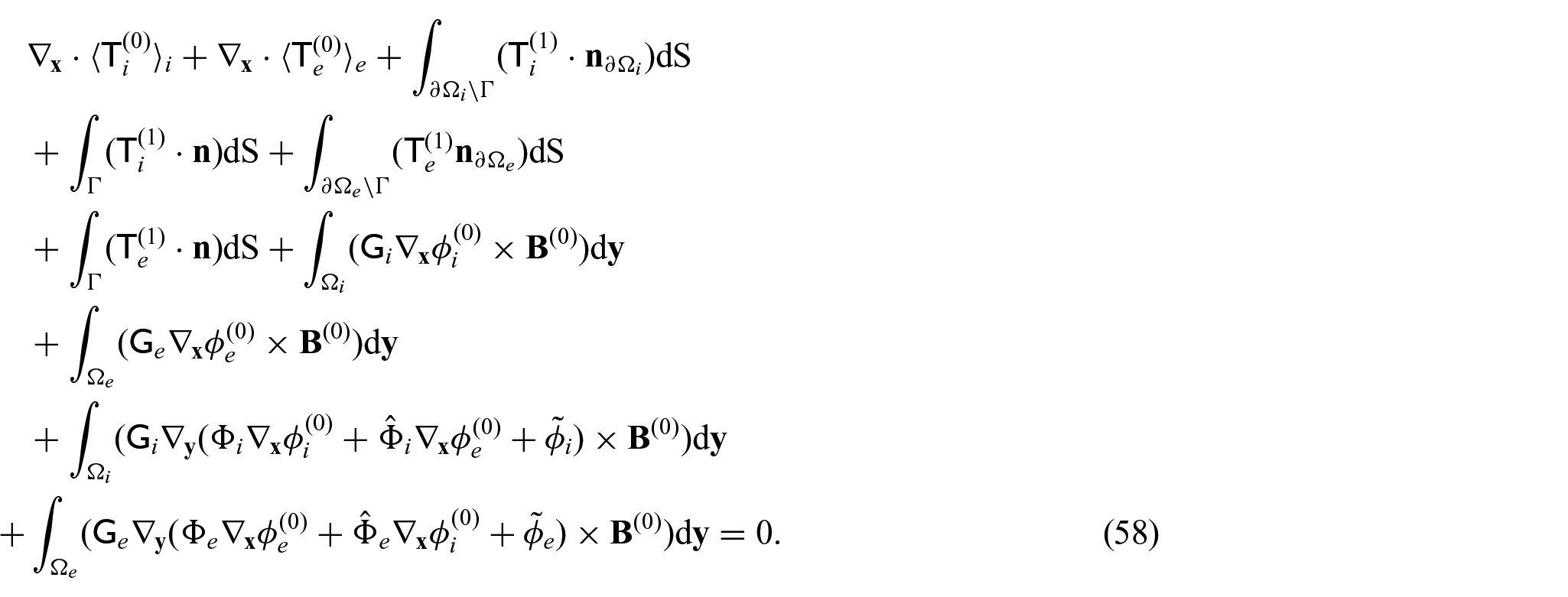
Now, we can take the integral average of the sum of equations (43a) and (43b) to obtain:
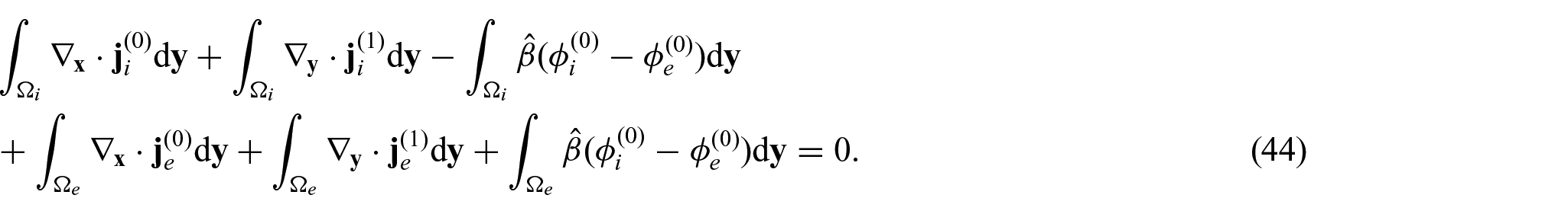
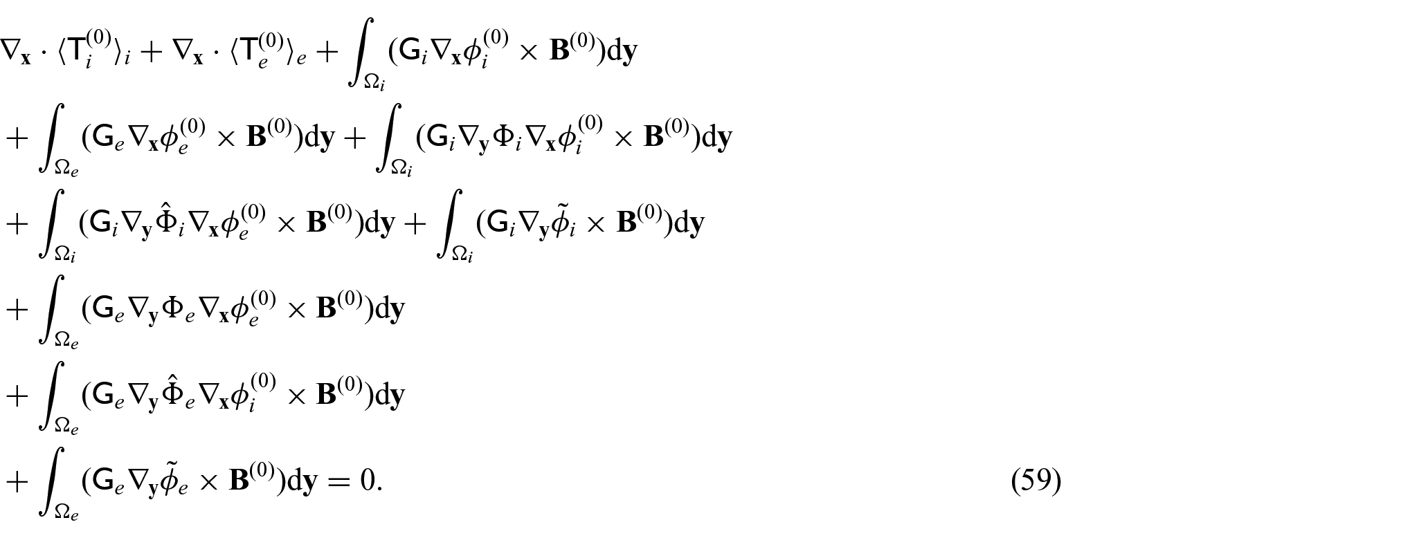
This can be rewritten as the following when applying macroscopic uniformity to the first and fourth integrals and the divergence theorem to the second and fifth integrals:
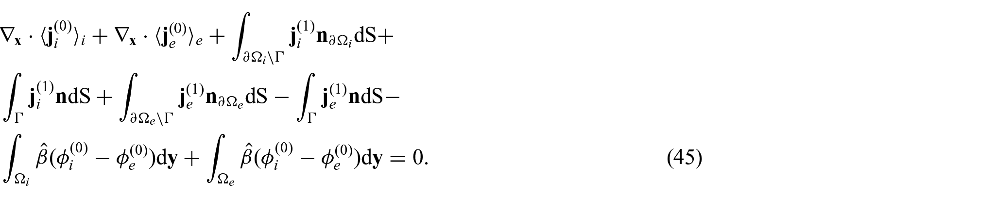
Due to periodicity, the terms on the external boundaries will cancel out, and using the

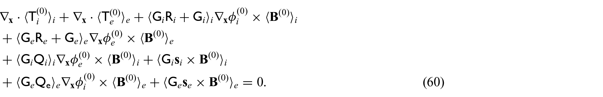
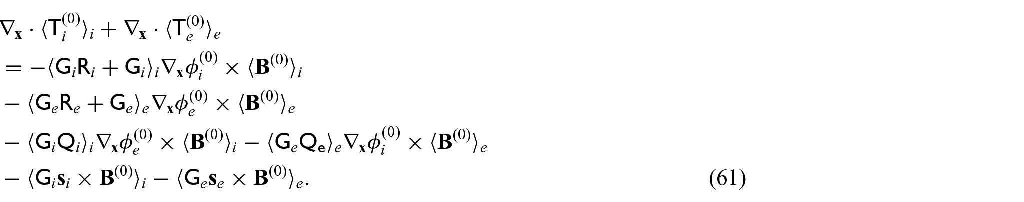
Since we have equations (24f) and (29a) and (29b), we can rewrite equation (46) as:

where


3.5. Problem for the elastic displacements
and
We now require a problem for


Since we have condition (26),


We can exploit the linearity of the problem to propose the ansatz:


where


For uniqueness of solution, we require an additional condition on the auxiliary tensors

Using the expressions, we have just obtained for

and

where we have used the notation:

We now want to consider a balance equation that takes into consideration each compartment. Taking the integral average of equations (31g) and (31h) gives:
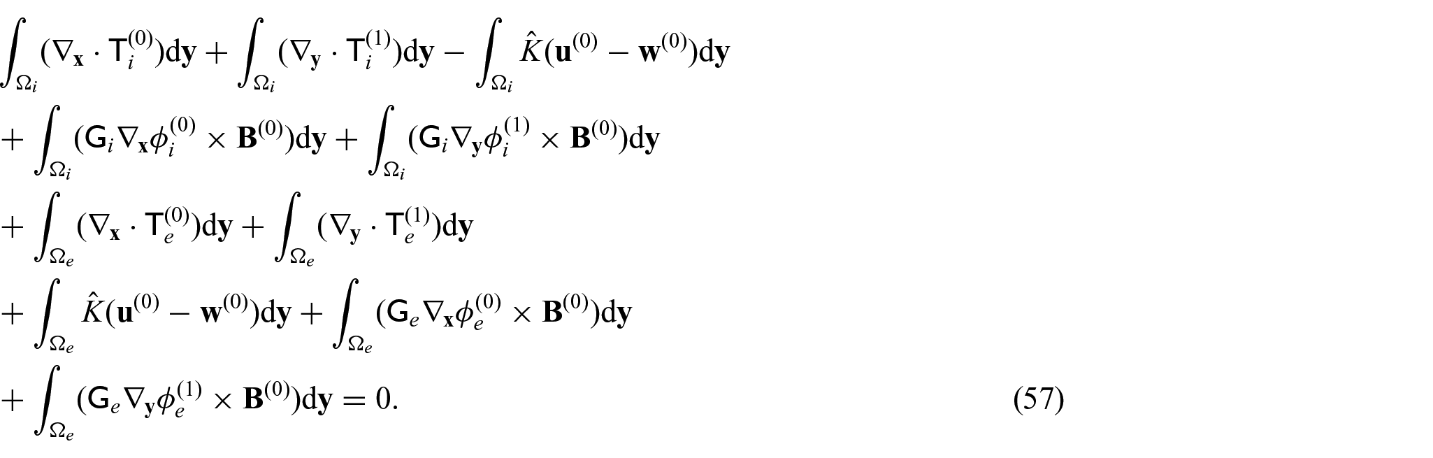
Since we have that
The terms of the external boundaries cancel due to periodicity and the terms on
Collecting integrals together and using the notation (40), we have:
This can then be written as:
We have now derived all the equations required to be able to state our macroscale model.
4. Macroscale model
The macroscale equations describe the effective behavior of the heart in terms of the leading order elastic displacement

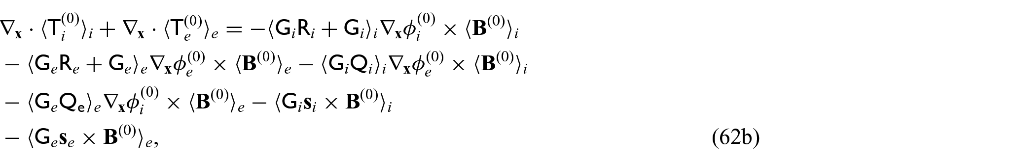

where we have the averaged leading order current densities:


and the averaged leading order solid stresses:


The novel model comprises the balance equation for the leading order current densities (62a). The current densities (63a) and (63b) comprise both the electric fields of each compartment premultiplied by second rank tensors that are to be obtained by solving the cell problems (34a)–(34d) and (35a)–(35d) and a vector term that arises from premultiplying the solutions to the cell problem (36a)–(36d) by the conductivity tensors. These coefficients arising from the cell problem solutions account for the differences in the electric potentials at each point in the microstructure and encode these in the model. We also have the balance equation for the solid stresses (62b), where the stresses are (64a) and (64b) with the standard effective elasticity tensors
5. Limit case and scheme to solve the model
In this section, we will consider some modifications to the model setup and the outcome they will have on the cell problems and overall model. We will also propose a scheme that can be used to solve the macroscale model.
5.1. Limit case here
Throughout this work, we have assumed that there is a potential drop
Under this assumption, the macroscale equation (62c) will become:

We can then consider the problem (32a)–(32d) assuming


We can use the fact that

We can then propose the following ansatz:


where


This is a vector problem which is driven by the difference in the conductivity tensors on the normal to the interface between the phases.
We can also use this ansatz to determine the current densities

and

The macroscale balance equation for the current densities (62a) can be simplified to:

The leading order solid stresses will remain unchanged as in equations (64a) and (64b) while the balance of the solid stresses (62b) will simplify to:

This means that we can summarize the simplified macroscale model using equations (72), (73), and (65) with amended leading order current densities (70) and (71) and the unchanged leading order solid stresses (64a) and (64b).
5.2. Scheme for solving the macroscale model
We now propose a scheme that can be implemented to solve the macroscale model (62a)–(62c). We progress in a step-by-step manner explaining how to find the effective model coefficients. We also explain how these coefficients will be used in later steps when solving the macroscale model (62a)–(62c). The model coefficients encode the structural details such as geometry, elastic, and electrical properties. Since we have assumed macroscopic uniformity of the material (see Remark 2) and assumed that the two scales are fully decoupled, then we can propose the following steps to solve the model. The process is as follows:
1. The first step is to set the original material properties of the intracellular and the extracellular domains at the microscale. We choose to make the assumption that each of the domains is isotropic. This means we require two parameters for each domain. These are two independent elastic constants that can be Poisson’s ratio and Young’s modulus (or alternatively the Lamé constants). We could, however, not make this assumption and just provide the elasticity tensor with up to 81 components depending on the symmetry that exists in each phase. We also must fix the original electrical properties such as the conductivity tensors in each phase with up to nine components and the potential drop
2. We must determine the microscale geometry; this includes defining the specific geometry of a single periodic cell and the volume of each of the phases.
3. We now begin the process that allows us to determine the macroscale model coefficients. We will begin with the elastic coefficients. We are able to solve the elastic-type cell problem (52a)–(52d) which has the solution auxiliary tensors


The solution to problem (74a)–(74d) is found by fixing the couple of indices
4. We now will solve the problems that will allow us to determine the tensors and vectors that contribute to the coefficients in the electrical current densities. We have the problems in components:


and


and


where we have used the notation:


The problems (76a)–(76d) and (77a)–(77d) are the vector problems. These have driving forces of conductivity tensor of each phase applied to the normal of the interface. The problem (78a)–(78d) is a scalar problem.
5. When solving the cell problems, we need the solution to be unique. We therefore require one additional condition. We make the choice that the cell averages of the auxiliary variables are zero. That is:

6. The auxiliary second rank tensors and vectors arising from the cell problems (
7. The structure and geometry of the macroscale must be set. This includes giving boundary conditions for the homogenized cell. We also must provide initial conditions for the macroscale solid elastic displacement and the electric potential drop
8. Finally, after carrying out all the above steps, our macroscale model (62a)–(62c) can then be solved.
6. Conclusion
In this work, we have derived a novel system of PDEs describing the effective electrical and mechanical behavior of an elastic composite designed to represent the myocardium tissue. Our structure comprises an elastic matrix, known as the extracellular domain, and embedded elastic subphases, known as the intracellular domain. This structure has been designed to account for the cardiac myocytes that are surrounded by a matrix which creates the heart muscle.
In order to derive the new model, we set up a microscale problem that describes the electrical and mechanical interactions between the cardiac myocytes and the surrounding matrix. We close the problem by accounting for the continuity of current densities, stresses and elastic displacements as well as the difference in the electric potentials across the interface between the myocyte and the matrix. We consider the heart muscle at a scale where the myocytes are distinct from the matrix. The microscale has an associated length much smaller than the one of the entire heart muscle (where we cannot see individual myocytes) and so the scale of the heart is known as the macroscale. Since we have this sharp scale separation, we are then able to apply the asymptotic homogenization technique to upscale the problem. The novel macroscale model that is derived is a first attempt at an asymptotic homogenization model for a coupled electrical and mechanical bidomain model. The novel model comprises balance equations for the current densities and for the stresses as well as additional terms accounting for the difference in the electric potentials at different points in the microstructure. The coefficients of the model encode the properties of the microstructure and are computed by solving the microscale differential problems arising as a result of applying the asymptotic homogenization technique.
The novel model obtained in this work is a first example of combining both the electrical and mechanical bidomain models of the heart via asymptotic homogenization. This can be considered as the next natural step in deriving computationally feasible electro-mechanical models for the heart based on the underlying microstructure. The key novelty of this work resides in considering how the mechanical deformations of the heart are influenced by the different electric fields arising from the electric potentials in each of the domains. The coupled cell problems (34a)–(34d), (35a)–(35d), as well as (36a)–(36d) encode the details of the difference in electric potentials at different points in the microstructure. The problem (52a)–(52d) is to be solved in order to obtain the tensors
This model is designed to describe the behavior of the heart and can be used in both healthy and diseased scenarios including growth and remodeling of cardiac tissue. We could use the model to investigate the displacement of the heart tissue due to the body forces that can be applied, such as the Lorentz force that we used in this work. This could provide some important results as the imaging of the elastic displacement due to Lorentz force has been recently proposed as a potential use of MRI [48]. This would allow traditional MRI to be used to measure bio-currents and differs from functional MRI that need to use blood oxygenation level-dependent signaling to detect currents [48].
The differences in intracellular and extracellular displacements that the new model includes can be considered to determine the role they play in mechanotransduction. This investigation would suggest whether a bidomain formulation, of the type in this work, is necessary when considering growth and remodeling. The mechanical element of the model can be used to predict tissue changes in the border zone surrounding a region of ischemia following myocardial infarction. It may also be considered when trying to explain why the complete heart muscle thickens during hypertrophy. In Puwal [49], the mechanical bidomain model has been used to predict how the heart responds to elevated blood pressure and other structural abnormalities.
Having a model that can describe the electrical activity of the heart is a very useful tool to aid the understanding of how the electrical function is impaired or changed by various diseases or disorders of the heart conduction system. With the novel model, we have derived here we can investigate how the structural changes caused by myocardial ischemia induce differences in the heart electrophysiology. The ischemia causes a change in the action potentials and the membrane potential increases with a larger uptake of potassium ions [50].
The current model assumes that both the matrix and myocytes are anisotropic linear elastic materials. We could, however, allow for these materials to be hyperelastic. This would involve a method similar to that carried out in Miller and Penta [51], Collis et al. [52], and Ramírez-Torres et al. [53]. Using nonlinear elasticity for the phases, we complicate the numerical simulations involved in computing the model coefficients and the macroscale model solution. The complication is due to the fact that the two length scales in the system remain coupled and massively increase the computational load. Recently, there has been the emergence of techniques to try to overcome this coupling of the scales (see Dehghani and Zilian [54, 55]).
By allowing for the matrix and myocytes to be hyperelastic, we could approach using nonlinear elasticity theory [56] and the Holzapfel–Ogden law [8]. This would allow us to treat the myocardium as a non-homogeneous, anisotropic, nonlinear elastic, incompressible material, with a strain energy function to describe the material. The parameters of the law would be to be determined by biological measurements using techniques such as those that have been investigated in Ogden et al. [57] and Gao [58]. Using such an approach, we could even consider the influence of residual stresses as investigated by Wang et al. [9] or different filling phases of the individual heart chambers [59].
In this work, we have assumed that both the myocyte and the matrix are anisotropic elastic solids. This could, however, be modified to provide slightly more realistic behavior of the phases. In Puwal and Roth [17], the assumption that the matrix is isotropic is made. This would be an easy enough modification to be made in this work. Puwal and Roth [17] assumed that the myocyte is not isotropic and therefore used a fluid-fiber continuum to represent the mechanical properties. They make the assumption that the myocardial fibers are directed along unit vectors which are in general a function of position. We can therefore modify the stress equation to comprise the intracellular pressure and the fiber tension. The fiber tension has two parts [60]: an active isometric tension at zero strain and a passive linear stress–strain relationship characterized by Young’s modulus. This allows for curving fibers in the myocyte to be accounted for as in Chadwick [60] and Holzapfel et al. [61]. These changes to the properties of the elastic phases could be incorporated in our model to improve the applicability to the heart and to provide a framework that can be used with experimental data.
The current work could be further developed in many ways, however, potentially the most important and useful of these would be to carry out the numerical simulations. This would mean obtaining solutions to the model using a specific microstructure with the parameters chosen by real-world data for the heart, myocytes, and electrical conductivity. Comparison between the numerical results and experimental data will allow for model validation and will give an insight into the predictive capabilities of the model as a potential diagnostic tool.
Footnotes
Funding
The author(s) disclosed the following financial support for the research, authorship, and/or publication of this article: R.P. is partially supported by EPSRC Grants EP/S030875/1 and EP/T017899/1 and conducted the research according to the inspiring scientific principles of the national Italian mathematics association Indam (“Istituto nazionale di Alta Matematica”), GNFM group.