Sage Journals: Discover world-class research

Abstract

The addition of nano-sized filler particles to polymers leads to significant improvements in their mechanical properties. These can be traced back to the matrix–filler interactions of the interphase, which can be analyzed using molecular dynamic simulations. Usually, research in this context studies the general number of entanglements or the radius of gyration. However, this publication presents a novel approach by investigating the radial distribution of entanglements in an effort to characterize the interphase. To this end, we employ a coarse-grained model for a generic polymer composite and study multiple systems with varying particle radius and matrix–filler adhesion. Furthermore, the highly customizable and computationally efficient nanocomposite system developed during this research serves as a foundation for the further characterization of polymer nanocomposites and their interphases.

Keywords

Molecular dynamics polymer nanocomposite interphase chain entanglement density distribution functions

1. Introduction

1.1. Motivation

Plastics make up one of the most important groups of materials to date. This is due to their broad application, low mass density, and cheap processing. The material group of polymer nanocomposites (PNCs) is especially attractive as their electrical, mechanical, thermal, and optical attributes can easily be altered by adding stiff fillers [1]. Compared to classical composites, the addition of nano-sized fillers leads to significant improvements in the mechanical properties at relatively small concentrations. However, it is often observed that the properties of PNCs cannot be accurately described by classical mixing rules [2, 3]. These take only the properties of the individual components into account and neglect the properties of the interphase. The interphase denotes the region close to a particle in which the material properties differ from the bulk because of the matrix–filler interaction. Due to the comparatively large surface-to-volume ratio in case of nano-sized fillers, the influence of these interphases may no longer be negligible and may cause their superior mechanical properties compared to classical (micro-)composites [4].

Therefore, it is of great importance to investigate the influence of nano-sized fillers on the properties of PNCs, especially in the close proximity of the nanoparticles (NPs). Only when this effect is fully understood, material properties of PNCs can be tailored on demand.

1.2. State of the art

A significant effort to characterize the interfacial layer of PNCs has been made, which will briefly be elucidated in the following. This section introduces methods and tools commonly used in this context. The overall structure of this brief overview is based on Ries et al. [5] and Liu et al. [6].

1.2.1. Experimental studies

Experimental studies regarding the micro-structure of PNCs are often conducted using small-angle scattering (SAXS/SANS) [7, 8] or transmission electron microscopy (TEM) [9, 10].

Furthermore, Brillouin light scattering (BLS) is often employed to analyze mechanical properties of the interfacial layer. Using BLS, Young’s modulus, Poisson’s ratio as well as the bulk and shear modulus of PNCs were measured [1, 11 –13]. These mechanical properties were also analyzed in relation to particle size and concentration. It was shown that the elastic modulus increases with growing NP concentration until a certain saturation is reached [14]. Mishra et al. observed that Young’s modulus is higher for composites with smaller particle size [15].

However, an accurate characterization of the interfacial region is difficult to realize experimentally because of superimposing NP interactions and non-ideally dispersed systems. Furthermore, there is no commonly established experimental procedure to measure properties at a specific location in a material.

1.2.2. Particle-based approaches

Since experimental studies cannot sufficiently approach the concept of the interphase, many numerical studies have been conducted. These can be divided into particle-based, continuum-based, and hybrid simulations. The methods of particle-based approaches are extensively described in Binder et al. [16], Frenkel and Smit [17], and Allen [18].

By employing Monte Carlo (MC) simulations, Papakonstantopoulos et al. [19, 20] found that the shear and Young’s moduli of PNCs are higher than in pure polymer samples. Shandiz and Montazeri [21] approximated the stiffness profile in the interphase by applying proper uniaxial tensile stress to zones of different density within the interfacial layer. In addition, using coarse-grained molecular dynamics (CGMD) approaches of polymer-silica nanocomposites, Rahimi et al. and Ghanbari et al. pointed out the influence of NPs on the structure of polymer chains. Their results show that the structure of chains in the interphase is different from the bulk because of the matrix–filler interaction [22 –24].

Particle-based approaches are very powerful to describe effects at the molecular level. However, molecular dynamics (MD) only studies small time windows and therefore cannot reach scales of classical engineering applications [25].

1.2.3. Continuum-based approaches

Continuum-based approaches consider the material as continuous, rather than as an assembly of discrete particles [26, 27]. Mortzavi et al. used a finite element (FE) approach to study the interphase effect on nanocomposites and found out that the effect is maximal for spherical fillers [28]. There have also been recent advances in the computational homogenization of nanocomposites. For example, Kumar et al. [29] captured the size effect by interface energetics–enhanced approaches and graded interphase–enhanced formulations. Continuum mechanics is very much the contrary to particle-based approaches since it is very effective regarding macroscopic interactions, but it reaches its limit at the microscopic scale [25].

1.2.4. Hybrid approaches

Hybrid simulations are employed in an effort to combine the advantages of particle-based methods on a molecular level with macroscopic continuum–based methods. A detailed introduction into multiscale modeling can be found in Pfaller [25].

An examplatory approach is the Capriccio method, which is a multiscale technique coupling a discrete MD domain and a continuum treated by FEs. Pfaller et al. [30] demonstrated the effectiveness of this coupling technique compared to FE by studying the strain of a nanocomposite with embedded silica NPs. It was demonstrated that a continuum-based approach only partially captures the observed strain inhomogeneities. The spatially varying mechanical properties in the interphase indeed require a particle-based approach. This technique was then employed by Ries et al. [5] to analyze the elastic and inelastic properties in the proximity of NPs via the interparticle strain.

1.3. Aim of this work

This paper provides a methodology to build a generic CGMD PNC system with high flexibility in terms of particle size and amount. To this end, the polymer system described in Dötschel et al. [31] was expanded and combined with the silica system built by Ries et al. [32]. These models were chosen as they are both thoroughly investigated and documented. Furthermore, the silica system is an ideal basis for a generic filler material as it possesses no symmetry due to its triclinic crystal structure [33]. The method presented in this research serves as a foundation for the further characterization of the properties of PNCs and the interphase.

This paper presents a novel approach to investigate the interphase by analyzing the radial distribution of chain entanglements. Most research in this context studies the general number of entanglements or the radius of gyration instead of their spatial distribution density (see [34 –36]). To achieve this, different systems with varying particle size and matrix–filler adhesion are analyzed here.

As this paper focuses on the interactions and position of molecules (Figure 1), a particle-based approach is used. As discussed in section 1.2, we regard MD as the most suited approach to understand effects on the molecular level.

Figure 1.

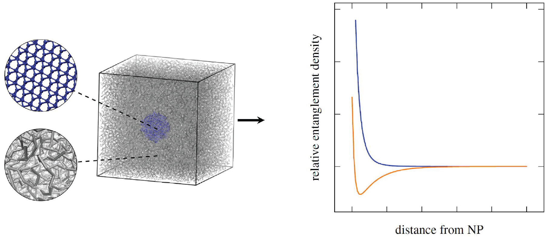
Graphical abstract: first, a generic CGMD PNC system is built from constituent systems. Second, the entanglement distribution density relative to the NP surface is analyzed.

1.4. Outline

The general structure of the paper is as follows. Section 2 presents the procedure of building a generic PNC. Furthermore, the analysis and graphical evaluation of said system using the Z1 algorithm is elaborated. The results of the graphical evaluation for multiple systems are discussed in section 3. Finally, section 4 concludes the paper and discusses possible enhancements along with providing an outlook to future research.

2. Methods

2.1. CGMD sample generation

This section describes the process of building a CGMD PNC model as summarized in Figure 2. First, the polymer model from Dötschel [31] is adapted to hold filler particles (see section 2.1.1). These NPs are obtained from the model built by Ries et al. [32]. The combination of these systems is described in section 2.1.2. To complete the modeling process, the reworked equilibration is outlined in section 2.1.3.

Figure 2.

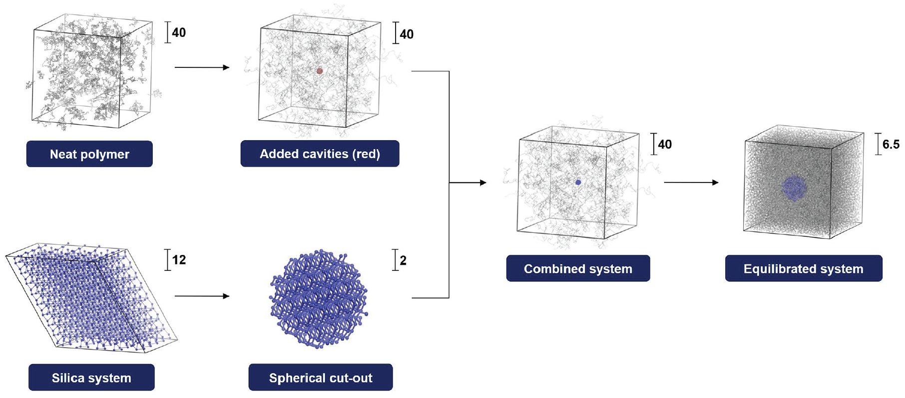
Workflow: spherical particles are cut from the silica system, scaled, rotated, and placed into the cavities defined within the neat polymer. Finally, the resulting system is equilibrated. All simulations use the unit-less generic models for filler particles and polymer matrix with the scaling indicated by numbers.

2.1.1. Self-avoiding random walk algorithm extension

First, we modify the original self-avoiding random walk (SARW) algorithm [31] in such a way that particles of arbitrary size and amount can be embedded into the system. In its current implementation, it considers only spherical particles since they are the easiest to study and also have the most optimal filler shape according to Mortazavi et al. [28].

The modified SARW starts by declaring the prospective positions of the NPs within the simulation box. The position can be set as random or to specific coordinates like the center of the simulation box. The position of the particle is automatically constrained such that the NPs neither overlap with each other nor protrude the simulation box. When choosing the size and number of particles, it is necessary to keep these variables within a reasonable relation to the box size to guarantee sufficient space for the polymer chains. Please note that composite systems with an extremely high filler concentration (>50 vol%) are beyond our scope, since the mechanical properties of PNCs do not increase beyond a certain amount of filler volume [14].

In the next step, the initial polymer chain atoms are declared. The algorithm ensures that no polymer atoms lie within the particle sphere. This additional spatial confinement is also checked during each step of the SARW. Furthermore, we found that it is not necessary to define the cavity bigger than the desired particle size to prevent initially high interaction potentials between the cut-out NPs and polymer atoms. As it turns out, the uneven surface of the NP ensures a minimal distance between atoms of the polymer and the filler particles, such that the interaction energies do not exceed feasible values. This will be considered further in section 2.2. After this step, we obtain the polymer at atomistic resolution with spherical cavities as given in Figure 2.

2.1.2. Insertion of particles

After adapting the SARW, the silica NPs have to be inserted into the polymer and a subsequent equilibration step is required. In order to prepare the filler particles, a silica crystal using normalized Lennard-Jones (LJ) units and periodic boundary conditions (PBCs) in all three coordinate directions is considered, out of which we cut a spherical subsystem. However, the particles created according to this procedure possess a highly irregular surface, which is most pronounced for small particles (Figure 3). Since such small fillers cannot be regarded any more as spheres as depicted in Figure 3(a) versus Figure 3(b), we thus do not consider filler particles with a radius smaller than 2.0.

Figure 3.

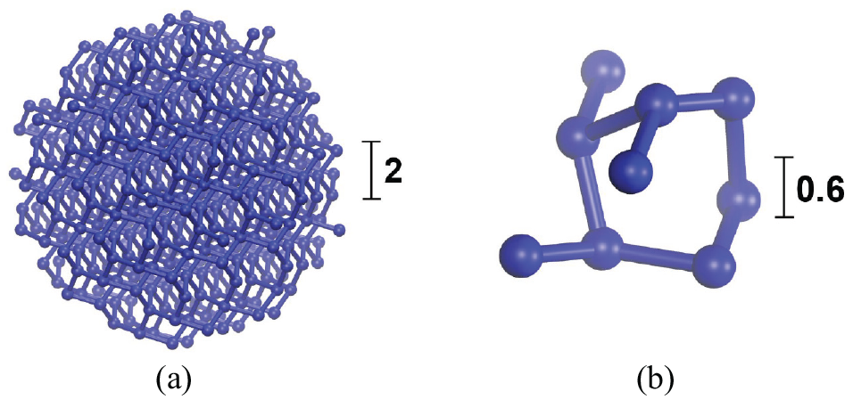
Nanoparticles: a visualization of a spherical NP with the radius of 5.0 (a) and a non-spherical NP with a cut-out radius of 1.5 (b); cut from the silica system. Note the different scales.

Since the silica model in our dimensionless setting is scaled differently than the polymer model ( $E_{\min, silica}^{b}$ for $r_{silica}^{b} = 3.2$ ), we have to downscale the silica to fit the potential used in the polymer model ( $E_{\min, polymer}^{b}$ for $r_{polymer}^{b} = 0.97$ ). This downscaling is performed by shrinking the simulation box accordingly. The required silica box length $ℓ$ in every dimension can be computed from the original length $ℓ_{0}$ as follows:

ℓ = \frac{E_{pot}^{polymer}}{E_{pot}^{silica}} \cdot ℓ_{0} .

(1)

Skipping this step would lead to extremely high initial interaction forces between the filler atoms. After rescaling the silica bonds, a sphere of equivalent size to the cavity in the polymer is carved out of the silica (see Figure 3(a)). As stated above, it is not necessary to define the cavity larger than the NP in order to minimize initial interaction forces.

In the next step, the NPs are randomly rotated and then inserted into the respective polymer sample created with the modified SARW. To this end, we rotate the particles about their centers by choosing random angles about three random directions. Subsequent averaging over all samples thus minimizes a resulting directional dependence arising from the filler anisotropy.

2.1.3. Equilibration

The equilibration of the PNC systems is based on the equilibration of the neat polymer by Ries et al. [33]. However, since the filler particles are introduced to the polymer model, the filler–filler and the matrix–filler interactions need to be defined. We employ a slightly modified adaptation of the equilibration process of Dötschel [31] by Ries et al. [33] to reduce computation time and improve the degree of entanglement. An overview of the normalized values is given in Table 1.

Table 1.

Additional CG interaction potentials due to added filler, based on Ries et al. [33]: values for bond angle and pair potentials.

	Bond	Angle	Pair
Filler–filler	Harmonic (6)	Cosine (7)	LJ (8)
based on Ries et al. [33]	$K = 3000$	$K = 100$	$ϵ = 1.0$
	$r_{0} = 0.89$		$σ = 1.0$
			$r_{c} = \sqrt[6]{2}$
Matrix–filler	-	-	LJ (8)
based on Ries et al. [33]			$ϵ = 1.0$ and $8.0$
			$σ = 1.0$
			$r_{c} = 2.5$
Matrix–matrix	Harmonic (5)	Cosine (7)	LJ (8)
based on Ries et al. [33]	$K = 30$	$K = 0.75$	$ϵ = 1.0$
	$R_{0} = 1.5$		$σ = 1.0$
	$ϵ = 1.0$		$r_{c} = \sqrt[6]{2}$
	$σ = 1.0$

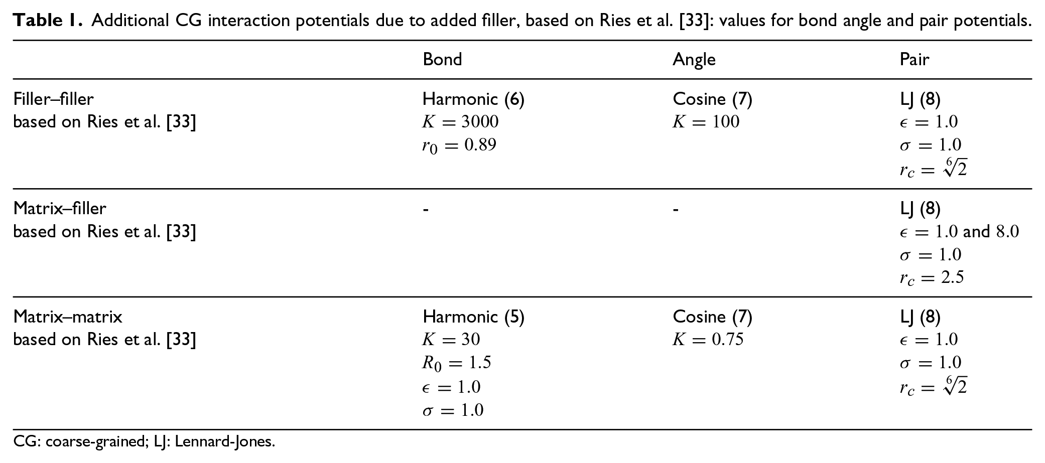
CG: coarse-grained; LJ: Lennard-Jones.

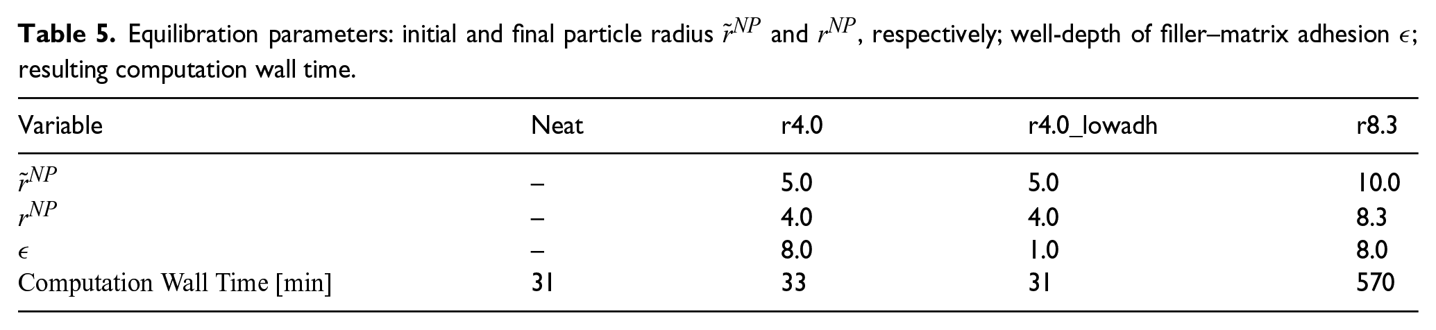
The equilibration is divided into three different phases, starting with an isothermal–isobaric ensemble at temperature $T = 1.0$ . Instead of holding the pressure at $p = 0$ , a pressure $p = 0.5$ is applied and linearly reduced over 100,000 time steps until the atmospheric pressure $p_{atm} = 0$ is reached. By this procedure, we enforce the chains to entangle with each other rather than to form separated balls of curled individual chains. Next, the system is cooled down to the temperature $T = 0.3$ over 140,000 time steps, which is below the glass transition temperature of $T_{g} \approx 0.41$ . Finally, the equilibration is concluded by holding the system at a temperature of $T = 0.3$ and a pressure of $p = 0$ for another 100,000 time steps [33].

Since the atoms forming the filler particles are cut from the periodic silica crystal, the atoms on the surface of the sphere now have less interaction partners. As evident from Table 2, the filler particle shrinks, which can be most likely traced back to the new surfaces generated by the cutting procedure. The NPs position also changes slightly, which will be addressed in the next section. An exemplary system after equilibration is depicted in Figure 2.

Table 2.

Particle radius alteration: initial particle radius ${\tilde{r}}^{NP}$ compared with the radius resulting from equilibration $r^{NP}$ .

${\tilde{r}}^{NP}$	$r^{NP}$
2.5	2.0
5	4.0
7.5	6.3
10	8.5

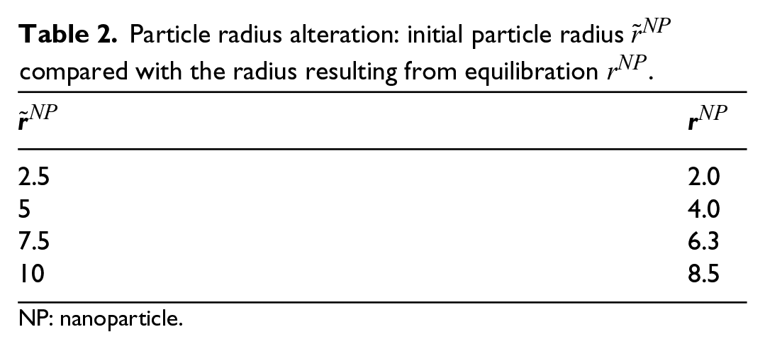
NP: nanoparticle.

2.2. Implementation of the Z1 algorithm

Based on the methodology introduced in section 2.1, we generate custom-tailored equilibrated PNC systems and analyze them thoroughly in the following. To this end, we employ the Z1 algorithm [34, 35, 37, 38] in an effort to study the radial distribution of polymer chain entanglements in relation to the NP surface to gather more information about the interphase. The Z1 algorithm analyzes a polymeric system and returns the shortest path alongside with the position and number of entanglements (see Figure 4). Furthermore, the algorithm allows the implementation of uncrossable obstacles and uses PBCs.

Figure 4.

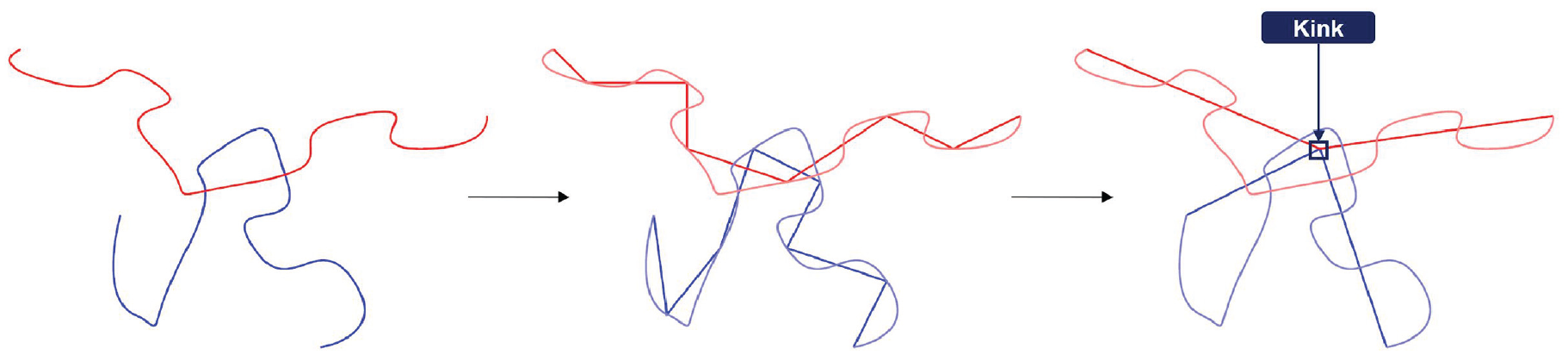
Schematic visualization of the path minimization of the Z1, based on Karayiannis and Kröger [38]: the two chains are minimized in end-to-end distance by reducing the bead count until the minimal path is found.

The Z1 algorithm requires obstacles to be in molecular form, meaning every bead is only allowed to have a single bond to another bead. This structure is also referred to as a dumbbell. Since this does not apply to the triclinic silica mesh, a conversion of the NP structure is necessary.

Since the path minimization of the Z1 algorithm is purely geometrical, the surface of the new NP structure needs to be much more dense than the original lattice. Otherwise, the polymer chains could slip through the holes in the NP surface during the execution of the algorithm. Furthermore, there is no need to place dumbbells inside the NP. Thus, it becomes clear that the NP can be replaced by a dense hollow sphere since the NPs considered in this publication are approximately spherical. This approximation is valid since the centroid and the center of mass for the NPs almost coincide.

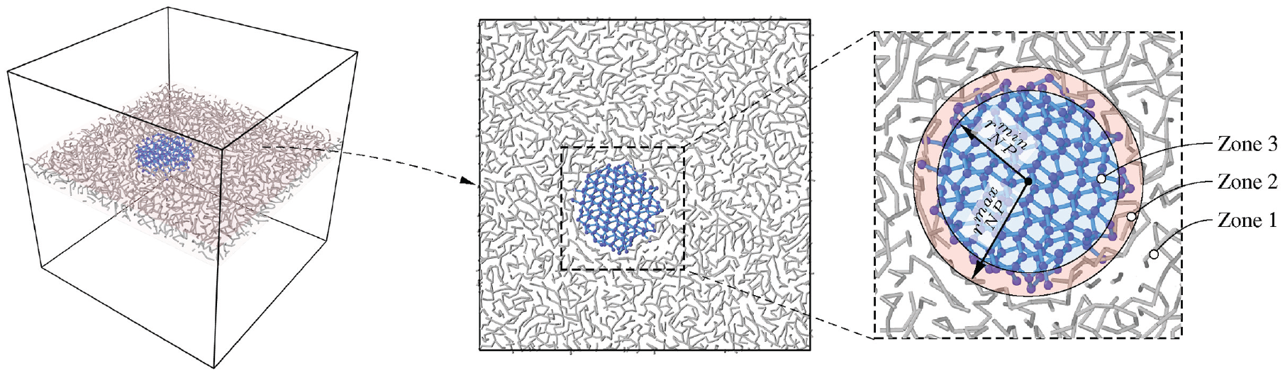
During equilibration, polymer chains fit tightly into the uneven surface of the NP. Thus, we can define three distinct zones: zone 1 $(r > r_{NP}^{\max})$ , where only polymer chains can be found, zone 2 $(r_{NP}^{\min} < r < r_{NP}^{\max})$ , which contains polymer and NP atoms, and finally, zone 3 $(r < r_{NP}^{\min})$ , which only includes particle beads (Figure 5).

Figure 5.

Definition of three distinct zones: zone 1 includes exclusively polymer beads, zone 2 contains polymer and particle beads, and finally, zone 3 only holds particle beads.

The radius of our replacement structure should be $r < r_{NP}^{\min}$ . Otherwise, parts of polymer chains would be trapped under the dense surface of dumbbells, which would locally increase the number of entanglements by almost 80 times.

In order to create a dense hollow sphere, we uniformly distribute points on a spherical surface using the Fibonacci spiral (see Figure 6). This algorithm was implemented by adapting a MATLAB script by Burkardt [39]. This algorithm was chosen since it is an easy way to uniformly distribute points on a sphere with a high degree of customization in a replicable fashion. For more detailed information about the Fibonacci sphere algorithm, the reader can refer to Swinbank and James Purser [40] and Saff and Kuijlaars [41].

Figure 6.

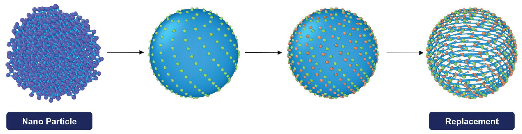
Visualization of the replacement of NPs: replacement of the NP with a dense hollow sphere consisting of dumbbells for the Z1 algorithm. For the purpose of visualization, significantly less dumbbells are used in this figure.

In order to create dumbbells, all Fibonacci points are copied and then rotated about the z-axis of the NP. An examplatory system is visualized in Figure 6. Every green point is bonded with its correlating rotated red partner. Even though there are still small slits between the bond lines, these are smaller than the defined thickness of the polymer chains during the Z1. Thus, the chains cannot penetrate the NP surface in any way. To guarantee this density, the user has to adapt the number of points according to the NP diameter. Also, the angle of rotation must be small enough to produce only bonds that are maximally five times longer than the average bond length of the system. Otherwise, the Z1 will not compile.

The algorithm now deletes all original particle information from the data file and overwrites them with the replacement. Thus, the NP is defined as a hollow sphere of radius $r_{NP}^{\min}$ with a dense surface during the Z1 algorithm.

2.3. Graphical evaluation

Among other quantities, the Z1 algorithm renders the kink coordinates. To investigate their arrangement in relation to the NP, a distribution function needs to be implemented. Simply plotting the number of kinks in relation to the NP radius in a histogram leads to flawed results as it is more likely to find more kinks in a histogram bin further away from the NP than in a bin closer to the surface. Thus, the position of the points was analyzed using a distribution function. A short introduction into the radial distribution function (RDF) and the cumulative distribution function (CDF) can be found in Appendix 1 (see section “Distribution functions”).

However, our systems differ from models classically analyzed with distribution functions. First, there is only one particle of interest instead of computing $g (r)$ for multiple particles. Second, due to the small volume of the simulation box, the volume of the NP cannot be neglected during the computation of $g (r)$ . It is therefore necessary to customize the distribution functions and find out which function is most suitable for the PNC model.

2.3.1. Reduction to a single evaluation point

Distribution functions are typically computed for each particle in the sample and normalized. Only computing the function from one point of interest introduces a lot of noise to the function. In an effort to visualize this, a cubic lattice with a bit of Gaussian noise added to the particle position is created, as shown in Figure 7. Now the RDF and the CDF are computed once for each particle in the system and once only from the origin, after making sure that there are no particles at (0 0 0). The resulting graphs are presented in Figure 8. By comparing these graphs, the function which is less prone to noise due to a singular evaluation point can be determined.

Figure 7.

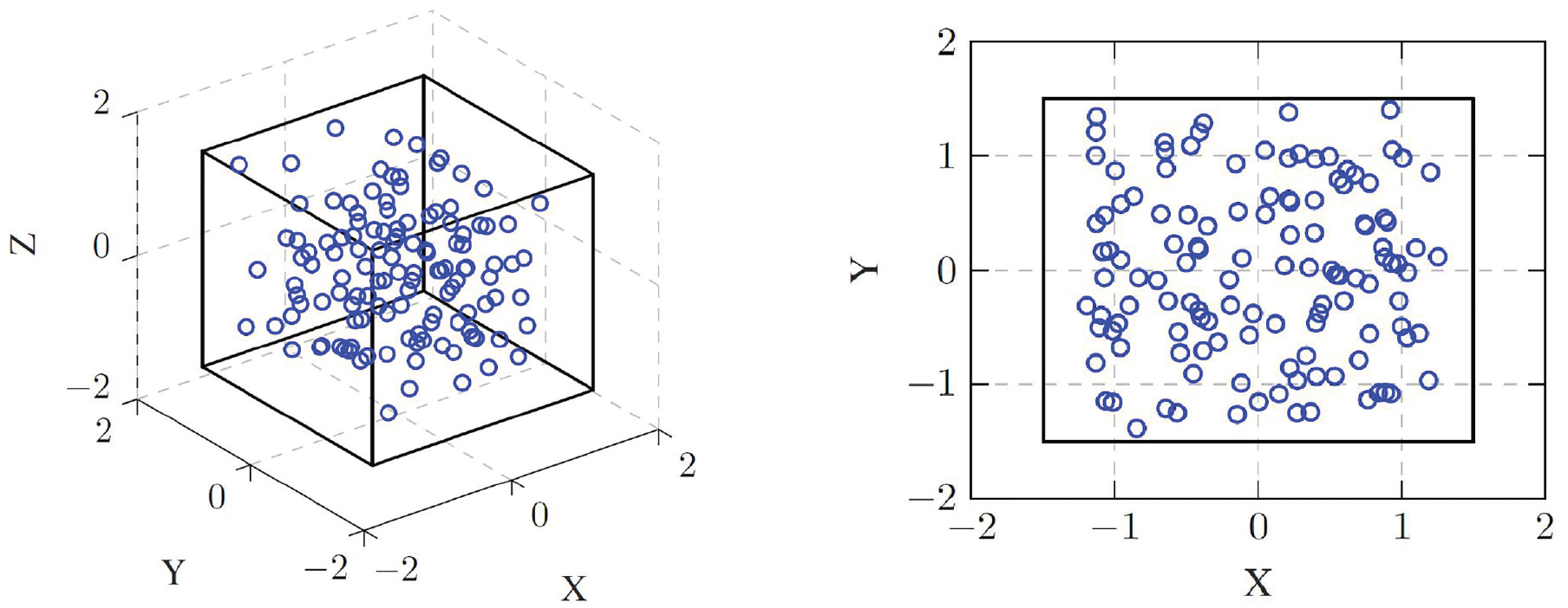
Visualization of cubic lattice with noise: small section out of the cubic lattice with distance 0.5 in 3D and 2D with added Gaussian noise.

Figure 8.

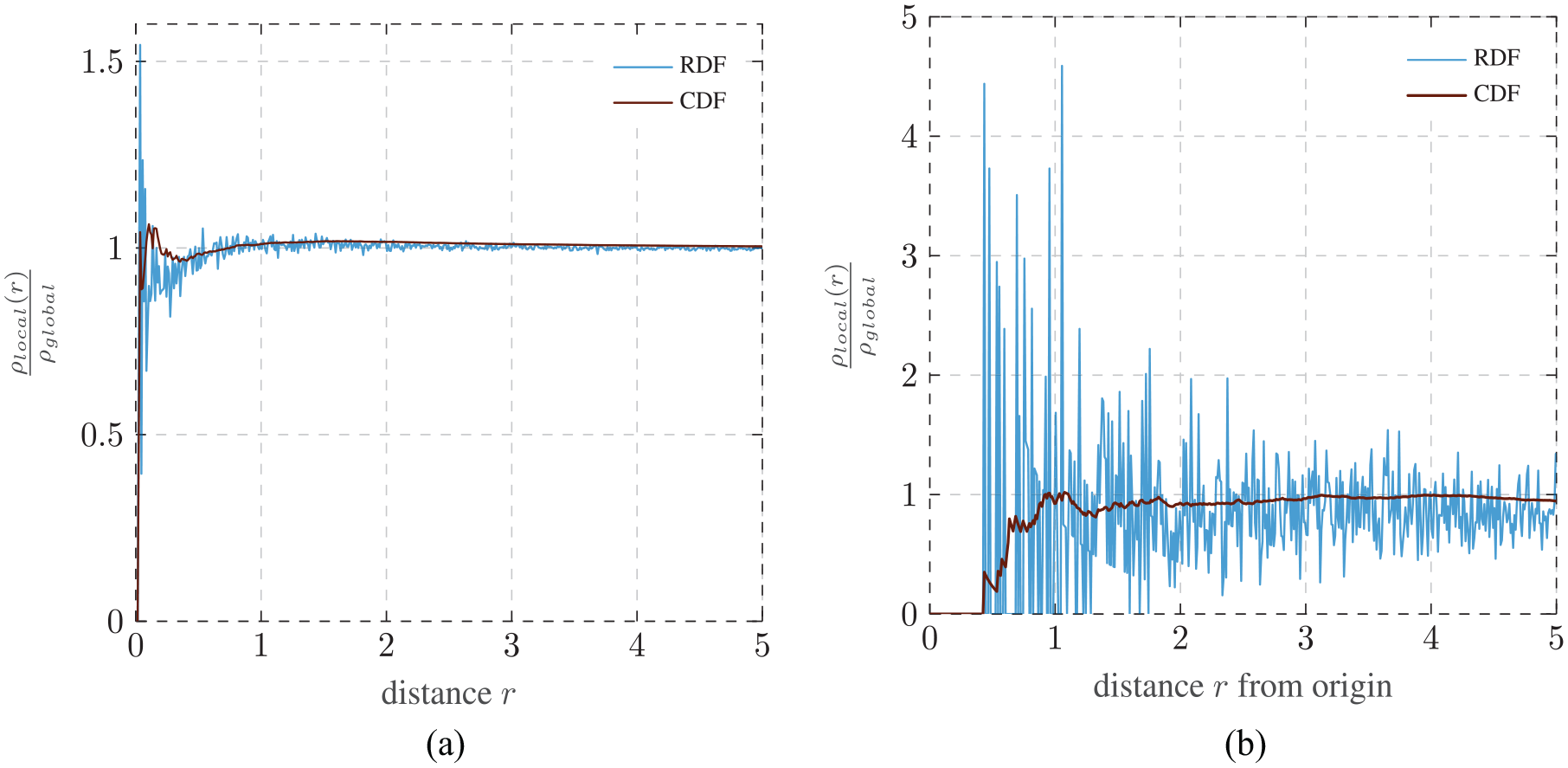
Influence of the number of evaluation points on the course of the radial and cumulative distribution functions: normalized over every particle (a); computed only from the origin (b).

The course of the RDF changes more drastically if the function is computed from only one point instead of averaging over every particle. Combined with the fact that the RDF is very sensitive to the bin width, the CDF is the more suitable distribution function. It should still be stated that the noise within the CDF is quite high, which causes a deviation between different sample systems. This noise can be reduced by averaging over the results of multiple systems.

2.3.2. Non-negligible volume

The second peculiarity of our system is that the volume of the NP cannot be neglected during the calculation of the CDF. This slightly alters the formulas of the CDF by introducing the condition $r > r_{NP}$ . First, the NP volume $V_{NP}$ needs to be subtracted from the subvolume $dV$ , resulting in:

V_{sphere} (r) = \frac{4}{3} π (r^{3} - r_{NP}^{3}), r > r_{NP} .

(2)

Second, we need to respect the volume of the particle during the normalization. This can be performed by subtracting $V_{NP}$ from $V_{global}$ as follows:

\begin{matrix} V_{global} = V_{box} - V_{NP} . \\ = ℓ_{box}^{3} - \frac{4}{3} π r_{NP}^{3} . \end{matrix}

(3)

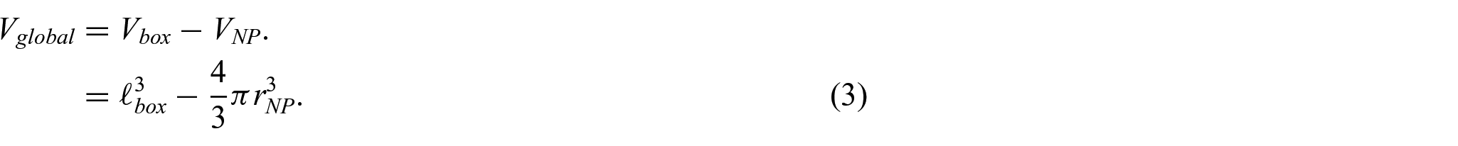
The rest of the computation remains the same.

3. Results

This section discusses the data resulting from the analysis of different systems regarding their spatial distribution of entanglements with the Z1 algorithm. First, the system parameters necessary to reproduce the data discussed in the following are specified in section 3.1. Then, section 3.2 considers the pure polymer system, whereas section 3.3 studies systems with a single NP with varying radii and adhesion forces. To distinguish the PNCs, we label them by “r” followed by the NP’s radius after equilibration. In addition, systems containing NPs with low adhesion are denoted by “lowadh.”

3.1. System parameters

We select the system parameters to be investigated such that we can study a representative range of PNCs in terms of particle radii and volume fractions of NPs at reasonable computational cost. When comparing systems with different NP sizes, it is important to keep a constant filler volume fraction:

ϕ^{NP} = \frac{V^{NP}}{V^{box}} .

(4)

Otherwise, the systems would not be comparable and the resulting curves would yield qualitatively different trends. However, keeping $ϕ^{NP}$ constant drastically increases the amount of simulated polymer beads with increasing particle size, as shown in Table 3.

Table 3.

Volume fractions $ϕ^{NP}$ for different systems.

NP radius	$4.0$	$8.3$	$8.3$
Box length after equilibration	$32$	$34$	$65$
Box volume	≈33,000	≈39,000	≈275,000
$ϕ^{NP}$	0.82 vol%	6.0 vol%	0.87 vol%
Number of chains	200	200	1 665
Number of beads	40,000	40,000	333,000

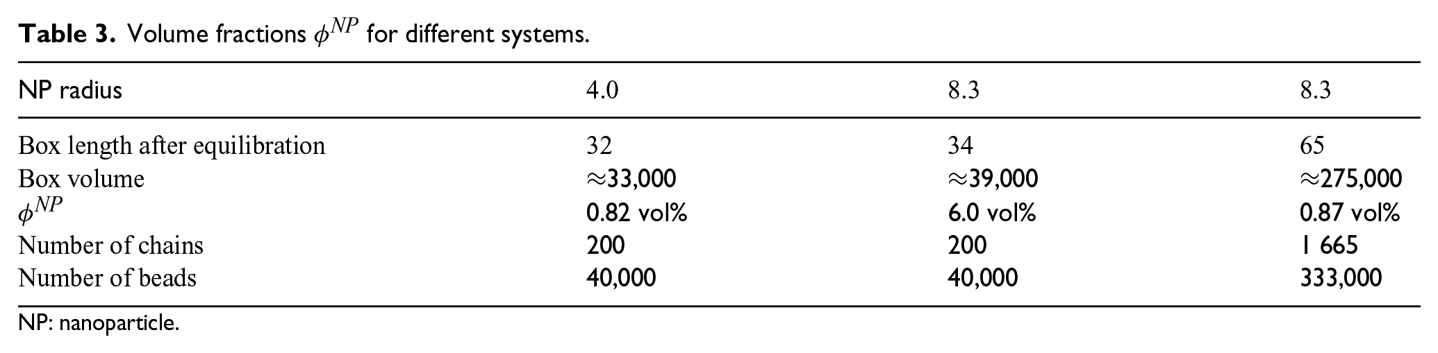
NP: nanoparticle.

In this contribution, particle sizes of $r = 4.0$ and $r = 8.3$ are investigated since larger particles are computationally too expensive. All other parameters of the SARW are summarized in Table 4. These parameters ensure the robustness for the SARW and equilibration. The box size for each system was set as small as possible. A half angle of $8 0^{°}$ proved to be the most robust choice. The large check was set to false as it was not deemed necessary. The step size and minimal non-bonded distance were kept at their standard values. These settings result from preliminary tests and are based on the findings of Dötschel [31].

Table 4.

Parameters for the self-avoiding random walker algorithm.

Variable	Neat	r4.0	r4.0_lowadh	r8.3
PartCount	0	1	1	1
PartSize before equilibration	–	5.0	5.0	10.0
N	200	200	200	1665
S	200	200	200	200
box	175	175	200	405
stepSize	1.0	1.0	1.0	1.0
minNonBonded	0.99	0.99	0.99	0.99
halfAngle	80	80	50	50
largeCheck	False	False	False	False
Computation Time [min]	9	10	10	540

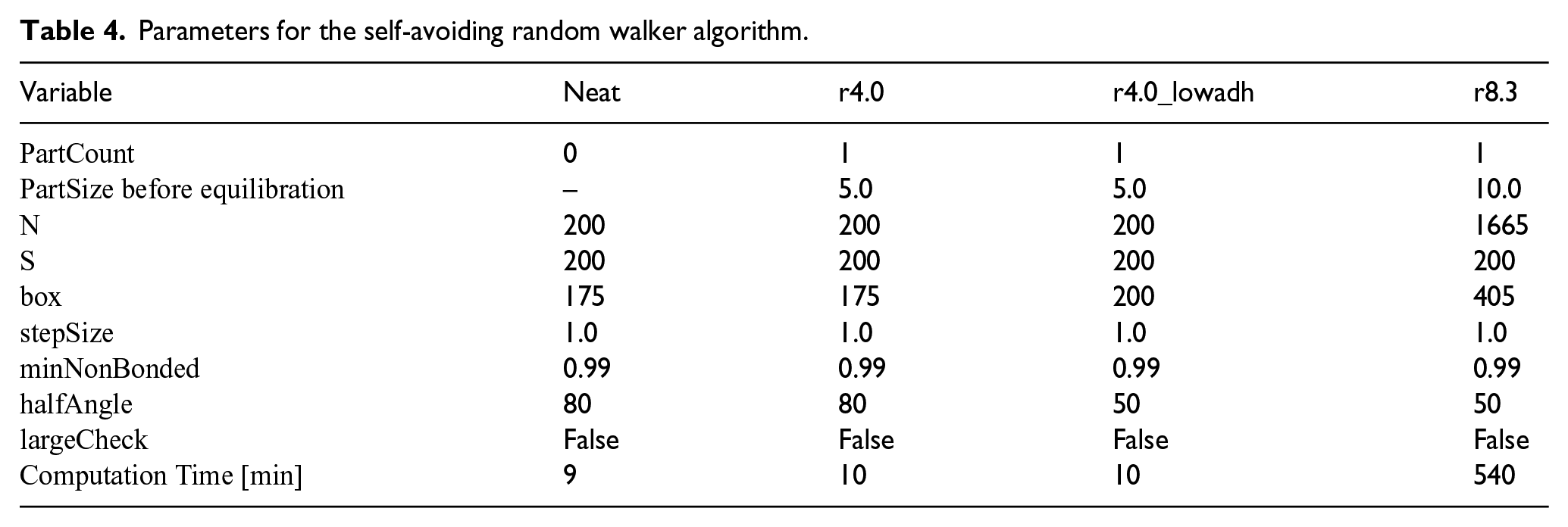
During the equilibration, the original radius ${\tilde{r}}^{NP}$ of the NPs changes slightly as already shown in Table 2. The reason for this is discussed in section 2.1.3. The impact of this trend on our systems as well as the average computation time for the equilibration is given in Table 5.

Table 5.

Equilibration parameters: initial and final particle radius ${\tilde{r}}^{NP}$ and $r^{NP}$ , respectively; well-depth of filler–matrix adhesion $ϵ$ ; resulting computation wall time.

Variable	Neat	r4.0	r4.0_lowadh	r8.3
${\tilde{r}}^{NP}$	–	5.0	5.0	10.0
$r^{NP}$	–	4.0	4.0	8.3
$ϵ$	–	8.0	1.0	8.0
Computation Wall Time [min]	31	33	31	570

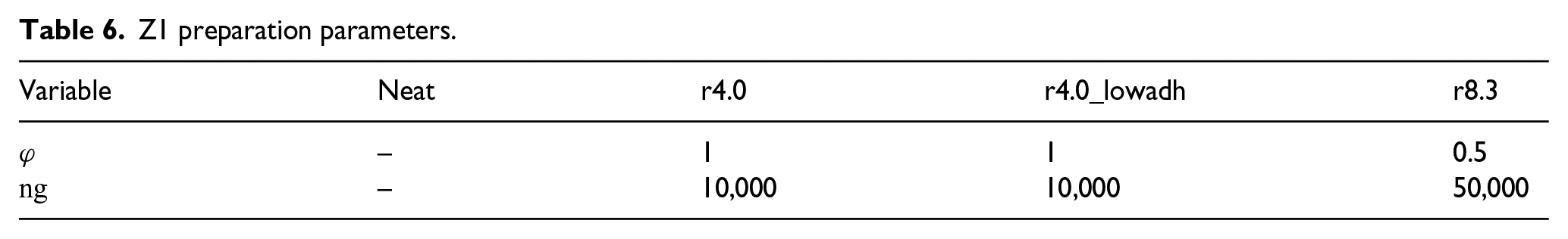
The only parameters that need to be set during the preparation of systems for the Z1 algorithm are the number of points on the surface of the Fibonacci sphere ng and their angle of rotation $φ$ . The values summarized in Table 6 turned out to be best suited for the systems under consideration.

Table 6.

Z1 preparation parameters.

Variable	Neat	r4.0	r4.0_lowadh	r8.3
$φ$	–	1	1	0.5
ng	–	10,000	10,000	50,000

3.2. Neat polymer

The first set of analyzed systems contains no NPs. This was performed in an effort to compare the neat polymer with the homogeneous system described in section 2.3.

Figure 9 shows the CDF averaged over 10 systems over the distance from the origin of the system with 100 histogram bins chosen. For radii smaller than 2, the CDF is zero meaning that there are no entanglements in none of the systems within such small distances from the origin. Most likely, this can be attributed to the low number of samples, which leads to a very low probability of encountering kinks in the smaller histogram bins. For radii larger than 2, the CDF initially increases at a large gradient, which tends to reduce when the CDF approaches 1. For radii between approximately 5 and 9, we observe rather high deviations from the ideal curve, which we also trace back to the low sample number.

Figure 9.

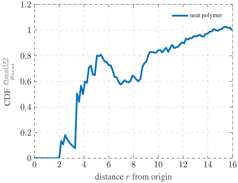
Cumulative distribution function (CDF) of the normalized entanglement density $ρ_{local}$ , normalized to the density of the neat polymer $ρ_{neat}$ as a function over the distance $r$ from the coordinate origin; the curve is the average over 10 neat polymer systems.

As expected, the graph is very similar to the CDF from the center of a homogeneous system with added noise in Figure 8. The spatial distribution of entanglements without any interference should be homogeneous. For a higher number of evaluated systems, this graph is expected to be even closer to Figure 8. This finding also serves as a confirmation of the implementation and analysis of the Z1 algorithm working as intended and allows the analysis of nanocomposite systems in the next section.

3.3. Nanocomposites

This section discusses the influence of the particle radius and the adhesion force by comparing the systems r4.0, r4.0_lowadh, and r8.3 in Figures 10 and 11, respectively. Contrary to the neat polymer, the CDF starts at the surface of the NP. The reasoning behind this approach is elaborated upon in section 2.3.

Figure 10.

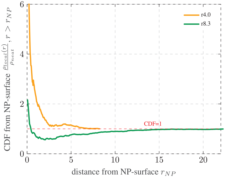
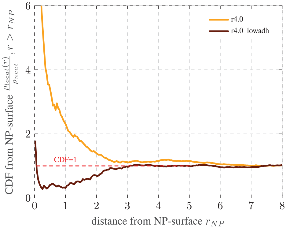
Impact of filler radius: CDF of the local entanglement density $ρ_{local}$ , over the distance from the NP-surface $r_{NP}$ , normalized to the density of the neat polymer $ρ_{neat}$ ; for NP radius, $r_{NP} = 4.0$ and $r_{NP} = 8.3$ .

Figure 11.

Impact of adhesion: CDF of the local entanglement density $ρ_{local}$ , over the distance from the NP-surface $r_{NP}$ , normalized to the density of the neat polymer $ρ_{neat}$ .

3.3.1. Influence of particle radius

The graph of the system r4.0 depicted in Figure 10 can be described as an exponential regression of the CDF that converges at 1. This convergence starts remarkably earlier compared to the neat polymer in section 3.2. This shows that the introduction of NPs alters the course of the graph not just quantitatively, but also qualitatively.

The course of this graph also indicates the influence of the interphase. Clearly, the entanglement density in close proximity of the NP surface is higher relative to the global density. This aligns with studies observing a higher Young’s modulus in the interphase [5]. Since one NP increases the entanglement density locally, it would be the logical consequence for the global entanglement density to increase with more NPs.

We assume that the start of convergence indicates the end of the interphase region. For the $r_{NP} = 4.0$ , this renders an interphase thickness of 2.5 which is approximately $60$ % of the NP radius. Contrary, for $r_{NP} = 8.3$ , we observe a convergence at a distance of approximately 15 indicating an interphase thickness of $180$ % with respect to the filler radius. Moreover, the graph for the larger particle shows a region also below 1, which indicates that there is a smaller number of entanglements in the vicinity of the particle. However, as for the smaller particle, it achieves a value of one for larger distances from the surface.

To verify this, however, extended further studies are necessary: among others, an appropriate range of individual particle radii could provide further insights into the influence of the particle radius on the interphase extension and properties. Beyond this, a larger number of samples for each particle radius should form a more sound statistical basis. In this context, a reliable and reproducible criterion to identify the interphase region is yet to be specified.

3.3.2. Influence of adhesion force

Next, we evaluate the influence of the adhesion force by comparing the systems r4.0 and r4.0_lowadh in Figure 11 with regular and low adhesion, respectively. The graph for r4.0_lowadh falls sharply in the beginning, plateaus for a small distance at around 0.3, before it increases again until it finally converges at around 3. This still results in an interphase thickness of 3, which is equivalent to $\approx 60$ % of the NP radius. However, the course is qualitatively different to the r4.0 system with regular adhesion, as that system never fell under a relative density of 1.

Subject to extended studies proposed above, this behavior might result from a gradually increasing influence of the surface adhesion. In Figure 12, we plot the courses for the extreme cases of strong surface adhesion (yellow) and of the neat polymer (blue). If we take the sum of these two curves, we obtain a graph of similar course to r4.0_lowadh. The computation is very similar to the generation of the LJ potential from the attractive and repulsive parts. This, in fact, would render the case of low adhesion as a combination between the two cases.

Figure 12.

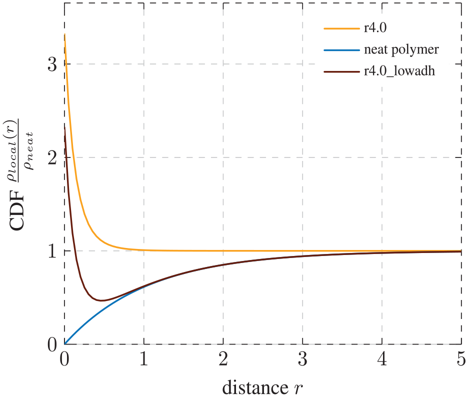
Combination of graphs: the course of the graph for radius of 4.0 with low adhesion can be described as a combination of the graphs for a neat polymer and a system with regular matrix–filler adhesion of radius 4.0

This is consistent with our theoretical understanding of the interphase. For small adhesion forces, the attraction zone in the LJ potential is very small (see equation (8)). Thus, only very few polymer chains would sense attraction from the NP. Polymer atoms further away from the NP would not be effected by the particle and, therefore, behave like in a neat system. This might cause the graph to look similar to a neat polymer system after a small distance from the surface. Furthermore, this would explain the quantitatively lower density directly on the surface of the NP.

4. Conclusion

This paper presents a detailed methodology of constructing a computationally efficient CGMD nanocomposite system based on Bocharova et al. [1], Dötschel [31], and Ries et al. [32]. In this process, multiple scripts were expanded and created. These scripts provide the user with many tools and adjustable parameters to allow for custom-tailored PNC systems.

Furthermore, the spatial density of polymer chain entanglement in relation to the NP surface was studied using the Z1 algorithm. This introduces a novel approach to the extensive research surrounding the interphase. In an effort to validate this methodology, multiple systems of varying particle size and adhesion were set up and studied.

By applying this algorithm, a qualitative influence of nano-sized particles on the chain topology of the nanocomposite was measured, which implies the existence of an interphase. Furthermore, our approach allows for an approximation of the interphase thickness by correlating the convergence of the CDF with the interphase size. For all systems, an increased entanglement density at the surface of the NP relative to the neat polymer was measured. This trend is heavily dependent on the size and adhesion of the added particle, which aligns with the results of other studies. For $r_{NP} = 4.0$ , we observe an interphase thickness of $60$ % of the filler radius independent of the adhesion force. However, for $r_{NP} = 8.3$ , the interphase reaches a thickness of $180$ % of the filler radius, indicating a size dependence.

This paper provides the basis for subsequent studies considering various particle radii and different surface adhesions. It would be possible to perform simulations with different filler volume percentages, interaction forces, and chain lengths. The systems provided by the methodology in this publication could also be analyzed regarding their gyration radius to compare the Z1 algorithm with more commonly used measurements. Currently, an extension of this model is also in progress, which analyzes the effect of chain grafting. To apply this model at engineering scale, it would be necessary to incorporate a multiscale coupling approach, like the Capriccio method [25].

5. Simulation software and data

The MD simulations were performed with LAMMPS [42, 43]. The simulations were performed on a high-performance computing resource, located at the Regional Computing Center Erlangen (RRZE). In the context of this research, one computing node with two Xeon 2660v2 “Ivy Bridge” chips (10 cores per chip) was used. MATLAB [44] was used to perform tensor calculus, to create, sort, and analyze data files, and to create graphics. Graphical evaluations of MD systems were also performed with Visual Molecular Dynamics (VMD) [45, 46].

Footnotes

Appendix 1 Funding

The author(s) disclosed receipt of the following financial support for the research, authorship, and/or publication of this article: This research was funded by the Deutsche Forschungsgemeinschaft (DFG, German Research Foundation) - 377472739/GRK 2423/2-2023. The authors are very grateful for this support. Sebastian Pfaller is funded by the Deutsche Forschungsgemeinschaft (DFG, German Research Foundation) - 396414850 (Individual Research Grant ‘Identifikation von Interphaseneigenschaften in Nanokompositen’).

ORCID iDs

Jakob Seibert

Maximilian Ries

References

Bocharova

Genix

Carrillo

JMY

, et al. Addition of short polymer chains mechanically reinforces glassy poly(2-vinylpyridine)–silica nanoparticle nanocomposites. ACS Appl Nano Mater 2020; 3(4): 3427–3438.

Cannillo

Bondioli

Lusvarghi

, et al. Modeling of ceramic particles filled polymer–matrix nanocomposites. Compos Sci Technol 2006; 66(7): 1030–1037, https://www.sciencedirect.com/science/article/pii/S0266353805002988

Reynaud

Jouen

Gauthier

, et al. Nanofillers in polymeric matrix: a study on silica reinforced PA6. Polymer 2001; 42(21): 8759–8768, https://www.sciencedirect.com/science/article/pii/S0032386101004463

Cho

Joshi

Sun

Effect of inclusion size on mechanical properties of polymeric composites with micro and nano particles. Compos Sci Technol 2006; 66(13): 1941–1952, https://www.sciencedirect.com/science/article/pii/S026635380600039X

Ries

Possart

Steinmann

, et al. A coupled MD-FE methodology to characterize mechanical interphases in polymeric nanocomposites. Int J Mech Sci 2021; 204: 106564, https://www.sciencedirect.com/science/article/pii/S002074032100299X

Liu

Pfaller

Rahimi

, et al. Uniaxial deformation of polystyrene–silica nanocomposites studied by hybrid molecular dynamics–finite element simulations. Comput Mater Sci 2017; 129: 1–12, https://www.sciencedirect.com/science/article/pii/S0927025616305924

Holt

Griffin

Bocharova

, et al. Dynamics at the polymer/nanoparticle interface in poly(2-vinylpyridine)/silica nanocomposites. Macromolecules 2014; 47(5): 1837–1843.

Holt

Bocharova

Cheng

, et al. Controlling interfacial dynamics: covalent bonding versus physical adsorption in polymer nanocomposites. ACS Nano 2016; 10(7): 6843–6852.

Ismail

Mustafa

, et al. Qualitative and quantitative analysis of intercalated and exfoliated silicate layers in asymmetric polyethersulfone/cloisite15A mixed matrix membrane for CO2/CH4 separation. Chem Eng J 2015; 268: 371–383, https://www.sciencedirect.com/science/article/pii/S1385894715001084

10.

Zhao

Senses

, et al. Role of filler shape and connectivity on the viscoelastic behavior in polymer nanocomposites. Macromolecules 2015; 48(15): 5433–5438.

11.

Cheng

Bocharova

Belianinov

, et al. Unraveling the mechanism of nanoscale mechanical reinforcement in glassy polymer nanocomposites. Nano Lett 2016; 16(6): 3630–3637.

12.

Holt

Bocharova

Cheng

, et al. Interplay between local dynamics and mechanical reinforcement in glassy polymer nanocomposites. Phys Rev Materials 2017; 1: 062601, https://link.aps.org/doi/10.1103/PhysRevMaterials.1.062601

13.

Zhao

Schneider

Fytas

, et al. Controlling the thermomechanical behavior of nanoparticle/polymer films. ACS Nano 2014; 8(8): 8163–8173.

14.

Rafiee

Wang

, et al. Enhanced mechanical properties of nanocomposites at low graphene content. ACS Nano 2009; 3(12): 3884–3890.

15.

Mishra

Sonawane

Singh

RP.

Studies on characterization of nano CaCO3 prepared by the in situ deposition technique and its application in PP-nano CaCO3 composites. J Polym Sci B 2005; 43(1): 107–113, https://onlinelibrary.wiley.com/doi/abs/10.1002/polb.20296

16.

Binder

Horbach

Kob

, et al. Molecular dynamics simulations. J Phys: Condens Matter 2004; 16(5): S429–S453.

17.

Frenkel

Smit

Understanding molecular simulation: from algorithms to applications, vol. 1. Amsterdam: Elsevier, 2001.

18.

Allen

MP.

Introduction to molecular dynamics simulation. Comput Soft Matter 2004; 23(1): 1–28.

19.

Papakonstantopoulos

Yoshimoto

Doxastakis

, et al. Local mechanical properties of polymeric nanocomposites. Phys Rev E 2005; 72: 031801, https://link.aps.org/doi/10.1103/PhysRevE.72.031801

20.

Papakonstantopoulos

Doxastakis

Nealey

, et al. Calculation of local mechanical properties of filled polymers. Phys Rev E 2007; 75: 031803, https://link.aps.org/doi/10.1103/PhysRevE.75.031803

21.

Shandiz

Montazeri

A novel MD-based procedure to obtain the interphase Young’s modulus in nanocomposites. Comput Mater Sci 2016; 113: 104–111, https://www.sciencedirect.com/science/article/pii/S0927025615007557

22.

Ghanbari

Rahimi

Dehghany

Influence of surface grafted polymers on the polymer dynamics in a silica–polystyrene nanocomposite: a coarse-grained molecular dynamics investigation. J Phys Chem C 2013; 117(47): 25069–25076.

23.

Ghanbari

Ndoro

TVM

Leroy

, et al. Interphase structure in silica–polystyrene nanocomposites: a coarse-grained molecular dynamics study. Macromolecules 2012; 45(1): 572–584.

24.

Rahimi

Iriarte-Carretero

Ghanbari

, et al. Mechanical behavior and interphase structure in a silica–polystyrene nanocomposite under uniaxial deformation. Proc Spie 2012; 23(30): 305702.

25.

Pfaller

Multiscale simulation of polymers—coupling of continuum mechanics and particle-based simulation. In: Steinmann

Willner

(eds) Schriftenreihe technische mechanik, vol. 16. Erlangen: Universität Erlangen-Nürnberg, 2015.

26.

Holzapfel

GA.

Nonlinear solid mechanics: a continuum approach for engineering science. Meccanica 2002; 37(4): 489–490.

27.

Willner

Kontinuums-und kontaktmechanik: synthetische und analytische darstellung. Berlin: Springer-Verlag, 2013.

28.

Mortazavi

Bardon

Ahzi

Interphase effect on the elastic and thermal conductivity response of polymer nanocomposite materials: 3D finite element study. Comput Mater Sci 2013; 69: 100–106, https://www.sciencedirect.com/science/article/pii/S0927025612006945

29.

Kumar

Steinmann

Mergheim

Enhanced computational homogenization techniques for modelling size effects in polymer composites. Comput Mech 2021; 68: 371–389.

30.

Pfaller

Possart

Steinmann

, et al. Investigation of interphase effects in silica–polystyrene nanocomposites based on a hybrid molecular-dynamics–finite-element simulation framework. Phys Rev E 2016; 93: 052505, https://link.aps.org/doi/10.1103/PhysRevE.93.052505

31.

Dötschel

Pfaller

Ries

Studying the mechanical behavior of a generic thermoplastic by means of a fast coarse-grained molecular dynamics model. Polym Polym Compos 2023; 31: 1–11.

32.

Ries

Bauer

Weber

, et al. Characterization of the material behavior and identification of effective elastic moduli based on molecular dynamics simulations of coarse-grained silica. Math Mech Solids 2022; 28: 1216–1231.

33.

Ries

Seibert

Steinmann

, et al. Applying a generic and fast coarse-grained molecular dynamics model to extensively study the mechanical behavior of polymer nanocomposites. Express Polym Lett 2022; 16: 1–19.

34.

Hoy

Foteinopoulou

Kröger

Topological analysis of polymeric melts: chain-length effects and fast-converging estimators for entanglement length. Phys Rev E 2009; 80: 031803, https://link.aps.org/doi/10.1103/PhysRevE.80.031803

35.

Hoy

Kröger

Unified analytic expressions for the entanglement length, tube diameter, and plateau modulus of polymer melts. Phys Rev Lett 2020; 124: 147801, https://link.aps.org/doi/10.1103/PhysRevLett.124.147801

36.

Moghimikheirabadi

Kröger

Karatrantos

AV.

Insights from modeling into structure, entanglements, and dynamics in attractive polymer nanocomposites. Soft Matter 2021; 17: 6362–6373.

37.

Kröger

Shortest multiple disconnected path for the analysis of entanglements in two- and three-dimensional polymeric systems. Comput Phys Commun 2005; 168(3): 209–232, https://www.sciencedirect.com/science/article/pii/S0010465505002808

38.

Karayiannis

Kröger

Combined molecular algorithms for the generation, equilibration and topological analysis of entangled polymers: methodology and performance. Int J Mol Sci 2009; 10(11): 5054–5089, https://www.mdpi.com/1422-0067/10/11/5054

39.

Burkardt

Sphere_ fibonacci_ grid, 2019, https://people.sc.fsu.edu/~jburkardt/m_src/sphere_fibonacci_grid/sphere_fibonacci_grid.html

40.

Swinbank

James Purser

Fibonacci grids: a novel approach to global modelling. Q J R Meteorol Soc 2006; 132(619): 1769–1793.

41.

Saff

Kuijlaars

AB.

Distributing many points on a sphere. Math Int 1997; 19(1): 5–11.

42.

Thompson

Aktulga

Berger

, et al. LAMMPS—a flexible simulation tool for particle-based materials modeling at the atomic, meso, and continuum scales. Comp Phys Comm 2022; 271: 108171.

43.

LAMMPS, 2022, https://www.lammps.org

44.

The Mathworks Inc. MATLAB, 2022, https://www.mathworks.com/products/matlab.html

45.

Humphrey

Dalke

Schulten

VMD—visual molecular dynamics. J Mol Graph 1996; 14: 33–38.

46.

Theoretical and Computational Biophysics Group. VMD, 2022, http://www.ks.uiuc.edu/Research/vmd/

47.

Younge

Christenson

Bohara

, et al. A model system for examining the radial distribution function. Am J Phys 2004; 72(9): 1247–1250.

48.

Kopera

BAF

Retsch

Computing the 3D radial distribution function from particle positions: an advanced analytic approach. Anal Chem 2018; 90(23): 13909–13914.

Investigation of the influence of nano-sized particles on the entanglement distribution of a generic polymer nanocomposite using molecular dynamics

Abstract

Keywords

1. Introduction

1.1. Motivation

1.2. State of the art

1.2.1. Experimental studies

1.2.2. Particle-based approaches

1.2.3. Continuum-based approaches

1.2.4. Hybrid approaches

1.3. Aim of this work

1.4. Outline

2. Methods

2.1. CGMD sample generation

2.1.1. Self-avoiding random walk algorithm extension

2.1.2. Insertion of particles

2.1.3. Equilibration

2.2. Implementation of the Z1 algorithm

2.3. Graphical evaluation

2.3.1. Reduction to a single evaluation point

2.3.2. Non-negligible volume

3. Results

3.1. System parameters

3.2. Neat polymer

3.3. Nanocomposites

3.3.1. Influence of particle radius

3.3.2. Influence of adhesion force

4. Conclusion

5. Simulation software and data

Footnotes

Appendix 1

Funding

ORCID iDs

References