Couple-stress–based gradient theory of poroelasticity

Abstract

In this research, we present a gradient theory of poroelasticity based on the couple-stress. Within the context of finite deformations and in a thermodynamically consistent manner, the constitutive equations for the porous solid are derived by including the solid vorticity gradient and its power-conjugate counterpart, namely, the couple-stress. Subsequently, a linearized theory for an isotropic porous solid is developed in which two microstructure-dependent constitutive moduli (or equivalently, two material length-scale parameters) are introduced. To investigate the gradient effects on the responses of the material, the problem of wave propagation in fluid-saturated porous solids is formulated and solved based on the proposed theory. For comparison, the wave dispersion and attenuation curves are compared with those obtained from classical theory of poroelasticity.

1. Introduction

The classical theory of poroelasticity concerns mechanical behavior of fluid-saturated porous solids at macroscales. Despite its wide range applications, the role of microstructure on the deformation of materials, which is believed to be dominant at small length scales, cannot be accounted for by the conventional theory. Besides, it has been uncovered that certain ill-posed problems can be prevented by including microstructure-related high-order terms [1,2]. During the past decades, a couple of size-dependent continuum theories, which involve internal material length scales, have been proposed to include the microstructure effects of the material. These theories fall roughly into two categories: high-order gradient theories [2–6] and Eringen’s nonlocal theories [7]. Based on these theories, the problems of one-dimensional consolidation of a porous layer [3,8] and wave propagation in porous media [9–11] have been examined. Besides, the high-order theories have been also applied to the study of the response of bone tissues (e.g., Giorgio et al. [5]).

Among high-order gradient theories, the couple-stress theory is an attractive one which has been used extensively to describe the size-dependent behaviors in solids. The origin of the couple-stress stems from Voigt [12], whereas the first couple-stress model for solids is proposed by Cosserat and Cosserat [13]. The modern frameworks of couple-stress theory are attributed to Grioli [14], Toupin [15,16], Mindlin and Tiersten [17], and Koiter [18] in which the vorticity gradient and the associated higher-order stress, say the couple-stress, are introduced to extend the classical theory of elasticity. More recently, a modified couple-stress model has been proposed by Yang et al. [19] by assuming the couple-stress being symmetric. A desirable feature of this model is that only one material length-scale parameter needs to be introduced.

The objective of this paper is twofold. First, to generalize the couple-stress theory of elasticity to the case of poroelasticity. Specifically, within the context of finite deformations and in a thermodynamically consistent manner, the constitutive equations for the porous solid are obtained by including the solid vorticity gradient and its power-conjugate counterpart, namely, the couple-stress. As in the conventional theory of poroelasticity, the saturating fluid is considered to be an elastic fluid with its free energy dependent only on the density. Furthermore, the linear couple-stress theory of poroelasticity for an isotropic porous solid is presented in which two microstructure-dependent constitutive moduli are introduced. The second objective is to investigate the gradient effects on the responses of the material. For this purpose, the problem of wave propagation in fluid-saturated porous solids is formulated and solved based on the proposed theory. To demonstrate the gradient effects, the wave dispersion and attenuation curves are compared with those obtained from classical theory of poroelasticity.

2. Kinematics

The saturated porous solid is composed of the porous skeleton and the saturating fluid. The former continuum is formed of solid particles and the latter continuum is formed of fluid particles. A solid particle and a fluid particle are superposed at the same geometrical point, whereas the solid and fluid continua have distinct kinematics.

To describe the kinematics of the solid skeleton, consider the porous solid is initially stress-free and occupies a region taken to be the reference configuration. A solid material point labeled by $\mathbf{X}$ in the reference configuration becomes the spatial point $\mathbf{x}=\mathbf{\chi }(\mathbf{X},t)$ in the current configuration. The deformation gradient $\mathbf{F}$ is defined by:

$$\mathbf{F}\equiv \frac{\partial \mathbf{\chi }}{\partial \mathbf{X}}=\mathbf{\chi }\otimes {\nabla }_{\mathrm{X}},$$

(1)

where ${\nabla }_{\mathrm{X}}$ , with a subscript $\mathrm{X}$ , denotes the nabla operator in the reference configuration and ⊗ denotes the tensor product of two vectors. In component form, $(\mathbf{F}{)}_{i\alpha }=\partial x_i/\partial X_{\alpha }$ Furthermore, note that ${\mathbf{F}}^{\mathrm{T}}={\nabla }_{\mathrm{X}}\otimes \mathbf{\chi }$ and $({\mathbf{F}}^{\mathrm{T}}{)}_{\alpha i}=\partial x_i/\partial X_{\alpha }$ .

To measure the pore volume change, we next introduce the Lagrangian porosity ${\varphi }_{\mathrm{R}}$ . Let $\varphi$ being the Eulerian porosity, then $\varphi \mathrm{d}{\mathrm{\Omega }}_t$ denotes the pore volume occupied in the current configuration, where $\mathrm{d}{\mathrm{\Omega }}_t$ represents the infinitesimal material volume in the current configuration. By contrast, the material porosity ${\varphi }_{\mathrm{R}}$ refers the current pore volume to the initial undeformed volume $\mathrm{d}{\mathrm{\Omega }}_0$ , which is defined by:

$$\varphi \mathrm{d}{\mathrm{\Omega }}_t={\varphi }_{\mathrm{R}}\mathrm{d}{\mathrm{\Omega }}_0.$$

(2)

By the relation:

$$\mathrm{d}{\mathrm{\Omega }}_t=J\mathrm{d}{\mathrm{\Omega }}_0,$$

(3)

with $J=det\mathbf{F}>0$ being the determinant of the deformation gradient tensor, we have:

$${\varphi }_{\mathrm{R}}=J\varphi .$$

(4)

In the initial undeformed state:

$${\varphi }_{\mathrm{R}}={\varphi }_0,$$

(5)

with ${\varphi }_0$ being the initial porosity.

3. Mass conservation

3.1. Solid mass conservation

For a material volume ${\mathrm{\Omega }}_t$ , the solid mass conservation requires:

$$\frac{{\mathrm{d}}^{\mathrm{s}}}{\mathrm{d}t}\underset{{\mathrm{\Omega }}_t}{\int }{\rho }_{\mathrm{s}}(1-\varphi )\mathrm{d}{\mathrm{\Omega }}_t=0,$$

(6)

where ${\rho }_{\mathrm{s}}$ is the intrinsic solid mass density, ${\mathrm{d}}^{\mathrm{s}}(•)/\mathrm{d}t$ denotes the Lagrangian/material time derivative with respect to solid particles (holding $\mathbf{X}$ fixed) and its relationship with the Eulerian/spatial time derivative $\partial (•)/\partial t$ (holding $\mathbf{x}$ fixed) is given by:

$$\frac{{\mathrm{d}}^{\mathrm{s}}(•)}{\mathrm{d}t}=\frac{\partial (•)}{\partial t}+\frac{\partial (•)}{\partial \mathbf{x}}·{\mathbf{v}}_{\mathrm{s}},$$

(7)

with ${\mathbf{v}}_{\mathrm{s}}(\mathbf{x},t)\equiv {\mathrm{d}}^{\mathrm{s}}\mathbf{x}/\mathrm{d}t$ being the velocity of the solid particle. Similarly, we may define the material time derivative with respect to fluid particles, i.e.,

$$\frac{{\mathrm{d}}^{\mathrm{f}}(•)}{\mathrm{d}t}=\frac{\partial (•)}{\partial t}+\frac{\partial (•)}{\partial \mathbf{x}}·{\mathbf{v}}_{\mathrm{f}},$$

(8)

with ${\mathbf{v}}_{\mathrm{f}}(\mathbf{x},t)\equiv {\mathrm{d}}^{\mathrm{f}}\mathbf{x}/\mathrm{d}t$ being the velocity of the fluid particle.

From equation (6), we obtain the local form:

$$\frac{\partial \left({\rho }_{\mathrm{s}}(1-\varphi )\right)}{\partial t}+\nabla ·\left({\rho }_{\mathrm{s}}(1-\varphi ){\mathbf{v}}_{\mathrm{s}}\right)=0,$$

(9)

where ∇, without a subscript, denotes the nabla operator in the current configuration.

3.2. Fluid mass conservation

Similarly, the fluid mass conservation can be expressed in the form:

$$\frac{{\mathrm{d}}^{\mathrm{f}}}{\mathrm{d}t}\underset{{\mathrm{\Omega }}_t}{\int }{\rho }_{\mathrm{f}}\varphi \mathrm{d}{\mathrm{\Omega }}_t=0,$$

(10)

where ${\rho }_{\mathrm{f}}$ is the intrinsic fluid mass density.

It follows from equation (10) the local form:

$$\frac{\partial \left({\rho }_{\mathrm{f}}\varphi \right)}{\partial t}+\nabla ·\left({\rho }_{\mathrm{f}}\varphi {\mathbf{v}}_{\mathrm{f}}\right)=0.$$

(11)

In the subsequent development, the Lagrangian fluid mass conservation equation will be used which can be written as [20]:

$$\frac{{\mathrm{d}}^{\mathrm{s}}{m}_{\mathrm{f}}}{\mathrm{d}t}+{\nabla }_{\mathrm{X}}·\mathbf{M}=0,$$

(12)

where $m_{\mathrm{f}}(\mathbf{X},t)={\rho }_{\mathrm{f}}{\varphi }_{\mathrm{R}}$ denotes the fluid mass content measured per unit reference volume; $\mathbf{M}(\mathbf{X},t)$ denotes the Lagrangian fluid mass flux measured per unit area per unit time and relates to its Eulerian counterpart $\mathbf{w}(\mathbf{x},t)\equiv {\rho }_{\mathrm{f}}\varphi ({\mathbf{v}}^{\mathrm{f}}-{\mathbf{v}}^{\mathrm{s}})$ via:

$$\mathbf{M}=J{\mathbf{F}}^{-1}\mathbf{w}.$$

(13)

4. Momentum balance equations

4.1. The equation of motion for the solid–fluid mixture

For an arbitrary material volume ${\mathrm{\Omega }}_t$ , in which both the solid and the fluid particles are included, balance of linear and rotational momentum requires:

$$\underset{\partial {\mathrm{\Omega }}_t}{\int }{\mathbf{t}}_n\mathrm{d}a+\underset{{\mathrm{\Omega }}_t}{\int }\mathbf{f}\rho \mathrm{d}{\mathrm{\Omega }}_t=\frac{{\mathrm{d}}^{\mathrm{s}}}{\mathrm{d}t}\underset{{\mathrm{\Omega }}_t}{\int }{\mathbf{v}}_{\mathrm{s}}{\rho }_{\mathrm{s}}(1-\varphi )\mathrm{d}{\mathrm{\Omega }}_t+\frac{{\mathrm{d}}^{\mathrm{f}}}{\mathrm{d}t}\underset{{\mathrm{\Omega }}_t}{\int }{\mathbf{v}}_{\mathrm{f}}{\rho }_{\mathrm{f}}\varphi \mathrm{d}{\mathrm{\Omega }}_t,$$

(14)

$$\underset{\partial {\mathrm{\Omega }}_t}{\int }(\mathbf{x}\times {\mathbf{t}}_n+{\mathbf{m}}_n)\mathrm{d}a+\underset{{\mathrm{\Omega }}_t}{\int }\mathbf{x}\times \mathbf{f}\rho \mathrm{d}{\mathrm{\Omega }}_t=\frac{{\mathrm{d}}^{\mathrm{s}}}{\mathrm{d}t}\underset{{\mathrm{\Omega }}_t}{\int }\mathbf{x}\times {\mathbf{v}}_{\mathrm{s}}{\rho }_{\mathrm{s}}(1-\varphi )\mathrm{d}{\mathrm{\Omega }}_t+\frac{{\mathrm{d}}^{\mathrm{f}}}{\mathrm{d}t}\underset{{\mathrm{\Omega }}_t}{\int }\mathbf{x}\times {\mathbf{v}}_{\mathrm{f}}{\rho }_{\mathrm{f}}\varphi \mathrm{d}{\mathrm{\Omega }}_t,$$

(15)

where ${\mathbf{t}}_n$ and ${\mathbf{m}}_n$ denote the force-stress and couple-stress vectors which act on the boundary $\partial {\mathrm{\Omega }}_t$ of ${\mathrm{\Omega }}_t$ ; $\mathbf{f}$ denotes the body force per unit mass; $\rho ={\rho }_{\mathrm{s}}(1-\varphi )+{\rho }_{\mathrm{f}}\varphi$ denotes the current mass density of the saturating material.

By the Cauchy tetrahedron argument, there exists a second-order, force-stress tensor $\mathbf{\sigma }$ such that:

$$\mathbf{\sigma }\mathbf{n}={\mathbf{t}}_n.$$

(16)

with $\mathbf{n}$ being the unit outward normal to $\partial {\mathrm{\Omega }}_t$ .

Similarly, we define a second-order, couple-stress tensor $\mathbf{\mu }$ by:

$$\mathbf{\mu }\mathbf{n}={\mathbf{m}}_n.$$

(17)

Substitution of equation (16) into equation (14) with use of the divergence theorem yields the macroscopic equation of motion (in the local form):

$$\mathbf{\sigma }·\nabla +{\rho }_{\mathrm{s}}(1-\varphi )(\mathbf{f}-{\mathbf{a}}_{\mathrm{s}})+{\rho }_{\mathrm{f}}\varphi (\mathbf{f}-{\mathbf{a}}_{\mathrm{f}})=0,$$

(18)

where ${\mathbf{a}}_{\mathrm{s}}(\mathbf{x},t)\equiv {\mathrm{d}}^{\mathrm{s}}{\mathbf{v}}_{\mathrm{s}}/\mathrm{d}t$ and ${\mathbf{a}}_{\mathrm{f}}(\mathbf{x},t)\equiv {\mathrm{d}}^{\mathrm{f}}{\mathbf{v}}_{\mathrm{f}}/\mathrm{d}t$ denote the acceleration field of solid and fluid particles; the divergence of $\mathbf{\sigma }$ is defined by $(\mathbf{\sigma }·\nabla {)}_i={\sigma }_{\mathrm{ij},j}$ .

In the same way, substitution of equations (16) and (17) into equation (15) and use of equation (18) leads to:

$$\mathbf{\mu }·\nabla -\mathbf{\sigma }\stackrel{\times }{·}\mathbf{I}=0,$$

(19)

where $\mathbf{I}$ denotes the second-order identity tensor and

$$\mathbf{\sigma }\stackrel{\times }{·}\mathbf{I}=({\sigma }_{\mathrm{ij}}{\mathbf{e}}_i\otimes {\mathbf{e}}_j)\stackrel{\times }{·}({\delta }_{\mathrm{pq}}{\mathbf{e}}_p\otimes {\mathbf{e}}_q)={\sigma }_{\mathrm{ij}}{\delta }_{\mathrm{pq}}({\mathbf{e}}_i\times {\mathbf{e}}_p)({\mathbf{e}}_j·{\mathbf{e}}_q)={ϵ}_{\mathrm{ipk}}{\sigma }_{\mathrm{ip}}{\mathbf{e}}_k,$$

(20)

with ${\delta }_{\mathrm{pq}}$ being the Kronecker delta and ${ϵ}_{\mathrm{ipk}}$ being the alternating symbol.

We now consider the decomposition of:

$$\mathbf{\sigma }=\mathbf{\tau }+{\mathbf{\tau }}^{°},$$

(21)

into the symmetric part $\mathbf{\tau }$ and the skew part ${\mathbf{\tau }}^{°}$ ; they are defined by:

$$\mathbf{\tau }\equiv \frac{1}{2}(\mathbf{\sigma }+{\mathbf{\sigma }}^{\mathrm{T}}),{\mathbf{\tau }}^{°}\equiv \frac{1}{2}(\mathbf{\sigma }-{\mathbf{\sigma }}^{\mathrm{T}}),$$

(22)

By equation (22), equation (19) simplifies to:

$$\mathbf{\mu }·\nabla -{\mathbf{\tau }}^{°}\stackrel{\times }{·}\mathbf{I}=0.$$

(23)

In addition, consider the decomposition of $\mathbf{\mu }$ into the sum of a deviatoric tensor and a spherical tensor, i.e.,

$$\mathbf{\mu }={\mathbf{\mu }}^{\mathrm{D}}+\frac{1}{3}\left(\mathrm{tr}\mathbf{\mu }\right)\mathbf{I},$$

(24)

with ${\mathbf{\mu }}^{\mathrm{D}}$ being the deviatoric part of $\mathbf{\mu }$ . Next, taking the curl of equation (23) with use of equation (24) yields:

$${\mathbf{\tau }}^{°}·\nabla =\frac{1}{2}\nabla \times ({\mathbf{\mu }}^{\mathrm{D}}·\nabla ).$$

(25)

Thus, by equation (25), the equation of motion (18) becomes:

$$\mathbf{\tau }·\nabla +\frac{1}{2}\nabla \times ({\mathbf{\mu }}^{\mathrm{D}}·\nabla )+{\rho }_{\mathrm{s}}(1-\varphi )(\mathbf{f}-{\mathbf{a}}_{\mathrm{s}})+{\rho }_{\mathrm{f}}\varphi (\mathbf{f}-{\mathbf{a}}_{\mathrm{f}})=0.$$

(26)

As is shown, the skew part of the force-stress tensor and the spherical part of the couple-stress tensor does not appear in the equation of motion and therefore are left indeterminate [17].

4.2. Equations of motion separate for the solid and fluid continua

The macroscopic force-stress $\mathbf{\sigma }$ represents the total stress acts on the representative elementary volume $\mathrm{d}{\mathrm{\Omega }}_t$ containing the whole matter, and it does not account for the stress related to the solid and the fluid continua. To identify their respective contributions, we may partition the total force-stress $\mathbf{\sigma }$ into:

$$\mathbf{\sigma }=(1-\varphi ){\mathbf{\sigma }}_{\mathrm{s}}+\varphi {\mathbf{\sigma }}_{\mathrm{f}},$$

(27)

with ${\mathbf{\sigma }}_{\mathrm{s}}$ and ${\mathbf{\sigma }}_{\mathrm{f}}$ being the macroscopic partial force-stress tensor related to the solid skeleton and the saturating fluid. Using a micro-macro averaging procedure, it can be shown that ${\mathbf{\sigma }}_{\mathrm{s}}$ and ${\mathbf{\sigma }}_{\mathrm{f}}$ are the averaged force-stress within the solid and the fluid (see Coussy [20,21] for details).

The saturating fluid is considered to be an elastic fluid, and hence, the force-stress ${\mathbf{\sigma }}_{\mathrm{f}}$ is a spherical tensor, so that:

$${\mathbf{\sigma }}_{\mathrm{f}}=-p\mathbf{I},$$

(28)

with $p$ being the pressure.

In addition, the macroscopic couple-stress $\mathbf{\mu }$ is solely related to the solid skeleton, irrespective with the saturating fluid, and hence:

$$\mathbf{\mu }=(1-\varphi ){\mathbf{\mu }}_{\mathrm{s}},$$

(29)

with ${\mathbf{\mu }}_{\mathrm{s}}$ being the averaged couple-stress within the solid skeleton.

Corresponding to the representation (27), the traction vector on the boundary $\partial {\mathrm{\Omega }}_t$ admits the partition:

$${\mathbf{t}}_{\mathrm{s}}+{\mathbf{t}}_{\mathrm{f}}={\mathbf{t}}_n,$$

(30)

where

$${\mathbf{t}}_{\mathrm{s}}=(1-\varphi ){\mathbf{\sigma }}_{\mathrm{s}}\mathbf{n},{\mathbf{t}}_{\mathrm{f}}=\varphi {\mathbf{\sigma }}_{\mathrm{f}}\mathbf{n}.$$

(31)

Furthermore, from equations (17) and (29), we have:

$${\mathbf{m}}_n=(1-\varphi ){\mathbf{\mu }}_{\mathrm{s}}\mathbf{n}.$$

(32)

Applying the linear momentum balance to the solid skeleton, we obtain the local equation of motion for the solid continuum in the form:

$$\left[(1-\varphi ){\mathbf{\sigma }}_{\mathrm{s}}\right]·\nabla +{\rho }_{\mathrm{s}}(1-\varphi )(\mathbf{f}-{\mathbf{a}}_{\mathrm{s}})+{\mathbf{f}}_{\mathrm{s}}^{\mathrm{int}}=0,$$

(33)

where ${\mathbf{f}}_{\mathrm{s}}^{\mathrm{int}}$ represents the macroscopic interaction force exerted by the fluid continuum. Furthermore, in view of equation (29) and

$${\mathbf{\tau }}^{°}=(1-\varphi ){\mathbf{\tau }}_{\mathrm{s}}^{°},$$

(34)

with ${\mathbf{\tau }}_{\mathrm{s}}^{°}$ being the skew part of ${\mathbf{\sigma }}_{\mathrm{s}}$ , the rotational momentum balance takes the form of equation (23).

For the saturating fluid, the local equation of motion becomes:

$$\left(\varphi {\mathbf{\sigma }}_{\mathrm{f}}\right)·\nabla +{\rho }_{\mathrm{f}}\varphi (\mathbf{f}-{\mathbf{a}}_{\mathrm{f}})+{\mathbf{f}}_{\mathrm{f}}^{\mathrm{int}}=0,$$

(35)

where ${\mathbf{f}}_{\mathrm{f}}^{\mathrm{int}}$ presents the macroscopic interaction force exerted by the solid phase and, by action and reaction law:

$${\mathbf{f}}_{\mathrm{s}}^{\mathrm{int}}+{\mathbf{f}}_{\mathrm{f}}^{\mathrm{int}}=0.$$

(36)

5. Constitutive theory

In the following development, the thermal effects are neglected and the purely mechanical theory is considered. Therefore, fields such as temperature, entropy, and heat flux are not mentioned.

5.1. Constitutive equations for the saturating fluid

For an elastic fluid, the specific free energy is only dependent on the density, i.e.,

$${\psi }_{\mathrm{f}}={\hat{\psi }}_{\mathrm{f}}\left({\rho }_{\mathrm{f}}\right),$$

(37)

where the “specific” indicates that ${\psi }_{\mathrm{f}}$ is measure per unit mass.

It follows from equation (37) that:

$$\frac{{\mathrm{d}}^{\mathrm{f}}{\psi }_{\mathrm{f}}}{\mathrm{d}t}=\frac{\partial {\hat{\psi }}_{\mathrm{f}}\left({\rho }_{\mathrm{f}}\right)}{\partial {\rho }_{\mathrm{f}}}\frac{{\mathrm{d}}^{\mathrm{f}}{\rho }_{\mathrm{f}}}{\mathrm{d}t}.$$

(38)

By the continuity equation:

$$\frac{{\mathrm{d}}^{\mathrm{f}}{\rho }_{\mathrm{f}}}{\mathrm{d}t}+{\rho }_{\mathrm{f}}\nabla ·{\mathbf{v}}_{\mathrm{f}}=0,$$

(39)

and equation (38), we find that:

$${\rho }_{\mathrm{f}}\frac{{\mathrm{d}}^{\mathrm{f}}{\psi }_{\mathrm{f}}}{\mathrm{d}t}=-{\rho }_{\mathrm{f}}^2\frac{\partial {\hat{\psi }}_{\mathrm{f}}\left({\rho }_{\mathrm{f}}\right)}{\partial {\rho }_{\mathrm{f}}}\nabla ·{\mathbf{v}}_{\mathrm{f}}=-{\rho }_{\mathrm{f}}^2\frac{\partial {\hat{\psi }}_{\mathrm{f}}\left({\rho }_{\mathrm{f}}\right)}{\partial {\rho }_{\mathrm{f}}}\mathbf{I}:{\mathbf{v}}_{\mathrm{f}}\otimes \nabla .$$

(40)

In addition, the constitutive relation is required to fulfill the free-energy imbalance, i.e., consistent with the second law of thermodynamics, if a purely mechanical theory is considered. By the free-energy imbalance, we arrive at (see, for example, Gurtin et al. [22]):

$${\rho }_{\mathrm{f}}\frac{{\mathrm{d}}^{\mathrm{f}}{\psi }_{\mathrm{f}}}{\mathrm{d}t}={\mathbf{\sigma }}_{\mathrm{f}}:{\mathbf{v}}_{\mathrm{f}}\otimes \nabla .$$

(41)

From equations (40) and (41), we obtain:

$${\mathbf{\sigma }}_{\mathrm{f}}=-{\rho }_{\mathrm{f}}^2\frac{\partial {\hat{\psi }}_{\mathrm{f}}\left({\rho }_{\mathrm{f}}\right)}{\partial {\rho }_{\mathrm{f}}}\mathbf{I}=-p\mathbf{I},$$

(42)

with the pressure $p=\hat{p}({\rho }_{\mathrm{f}})$ given by:

$$p={\rho }_{\mathrm{f}}^2\frac{\partial {\hat{\psi }}_{\mathrm{f}}\left({\rho }_{\mathrm{f}}\right)}{\partial {\rho }_{\mathrm{f}}}.$$

(43)

Differentiating equation (43) yields:

$$\frac{\mathrm{d}{\rho }_{\mathrm{f}}}{{\rho }_{\mathrm{f}}}=\frac{\mathrm{d}p}{K_{\mathrm{f}}},$$

(44)

where

$$K_{\mathrm{f}}\equiv {\rho }_{\mathrm{f}}^3(\frac{{\partial }^2{\hat{\psi }}_{\mathrm{f}}\left({\rho }_{\mathrm{f}}\right)}{\partial {\rho }_{\mathrm{f}}^2}+\frac{2}{{\rho }_{\mathrm{f}}}\frac{\partial {\hat{\psi }}_{\mathrm{f}}\left({\rho }_{\mathrm{f}}\right)}{\partial {\rho }_{\mathrm{f}}}),$$

(45)

denotes the fluid tangent bulk modulus.

Note that, as in the classical poroelasticity, the fluid free energy is given as a function of density in the proposed theory. By allowing the free energy to also depend on the density gradient, a second-grade fluid may be considered (see, for example, Seppecher [23] for more details).

5.2. Constitutive equations for the solid skeleton

We now turn to discuss the solid constitutive equations involving second gradients of deformation via the solid vorticity gradient. To begin with, we first define the power expanded within an arbitrary material volume ${\mathrm{\Omega }}_t$ , containing both solid and fluid particles, by:

$$\begin{array}{c}\multicolumn{1}{c}{\underset{{\mathrm{\Omega }}_t}{\int }{\mathrm{w}}^{\mathrm{int}}\mathrm{d}{\mathrm{\Omega }}_t\equiv \underset{\partial {\mathrm{\Omega }}_t}{\int }({\mathbf{t}}_{\mathrm{s}}·{\mathbf{v}}_{\mathrm{s}}+{\mathbf{m}}_n·{\mathbf{\omega }}_{\mathrm{s}}+{\mathbf{t}}_{\mathrm{f}}·{\mathbf{v}}_{\mathrm{f}})\mathrm{d}a+\underset{{\mathrm{\Omega }}_t}{\int }({\rho }_{\mathrm{s}}(1-\varphi )\mathbf{f}·{\mathbf{v}}_{\mathrm{s}}+{\rho }_{\mathrm{f}}\varphi \mathbf{f}·{\mathbf{v}}_{\mathrm{f}})\mathrm{d}{\mathrm{\Omega }}_t}\\ -\frac{{\mathrm{d}}^{\mathrm{s}}}{\mathrm{d}t}\underset{{\mathrm{\Omega }}_t}{\int }\frac{1}{2}{\mathbf{v}}_{\mathrm{s}}·{\mathbf{v}}_{\mathrm{s}}{\rho }_{\mathrm{s}}(1-\varphi )\mathrm{d}{\mathrm{\Omega }}_t-\frac{{\mathrm{d}}^{\mathrm{f}}}{\mathrm{d}t}\underset{{\mathrm{\Omega }}_t}{\int }\frac{1}{2}{\mathbf{v}}_{\mathrm{f}}·{\mathbf{v}}_{\mathrm{f}}{\rho }_{\mathrm{f}}\varphi \mathrm{d}{\mathrm{\Omega }}_t,\hfill \end{array}$$

(46)

where the internal power ${\mathrm{w}}^{\mathrm{int}}$ is measured per unit current volume and ${\mathbf{\omega }}_{\mathrm{s}}$ , power-conjugate to the couple-stress vector ${\mathbf{m}}_n$ , is the solid vorticity defined by:

$${\mathbf{\omega }}_{\mathrm{s}}=\frac{1}{2}\nabla \times {\mathbf{v}}_{\mathrm{s}}.$$

(47)

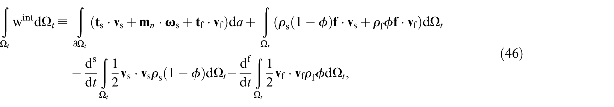
The internal power expenditure is defined as the external power expenditure, represented by the first two terms on the right-hand side of equation (46), minus the rate at which the kinetic energies are increasing. By the divergence theorem and balance equations (23), (33), and (35), the local form of equation (46) can be obtained in the form:

$${\mathrm{w}}^{\mathrm{int}}=\mathbf{\tau }:{\mathbf{d}}_{\mathrm{s}}+\varphi {\mathbf{\sigma }}_{\mathrm{f}}:({\mathbf{v}}_{\mathrm{f}}-{\mathbf{v}}_{\mathrm{s}})\otimes \nabla +{\mathbf{\mu }}^{\mathrm{D}}:({\mathbf{\omega }}_{\mathrm{s}}\otimes \nabla )-{\mathbf{f}}_{\mathrm{f}}^{\mathrm{int}}·({\mathbf{v}}_{\mathrm{f}}-{\mathbf{v}}_{\mathrm{s}}),$$

(48)

where ${\mathbf{d}}_{\mathrm{s}}$ denotes the symmetric part of solid velocity gradient. Solving equation (35) for ${\mathbf{f}}_{\mathrm{f}}^{\mathrm{int}}$ and substituting the result into equation (48) yields:

$${\mathrm{w}}^{\mathrm{int}}=\mathbf{\tau }:{\mathbf{d}}_{\mathrm{s}}+{\mathbf{\mu }}^{\mathrm{D}}:({\mathbf{\omega }}_{\mathrm{s}}\otimes \nabla )+\left(\frac{1}{{\rho }_{\mathrm{f}}}{\mathbf{\sigma }}_{\mathrm{f}}\mathbf{w}\right)·\nabla +(\mathbf{f}-{\mathbf{a}}_{\mathrm{f}})·\mathbf{w},$$

(49)

where use has been made of the relation:

$$[\left(\varphi {\mathbf{\sigma }}_{\mathrm{f}}\right)·\nabla ]·\left(\frac{\mathbf{w}}{\varphi {\rho }_{\mathrm{f}}}\right)=\left(\frac{1}{{\rho }_{\mathrm{f}}}{\mathbf{\sigma }}_{\mathrm{f}}\mathbf{w}\right)·\nabla -\varphi {\mathbf{\sigma }}_{\mathrm{f}}:({\mathbf{v}}_{\mathrm{f}}-{\mathbf{v}}_{\mathrm{s}})\otimes \nabla .$$

(50)

Equivalently, we may express equation (49) as:

$${\mathrm{w}}_{\mathrm{R}}^{\mathrm{int}}=J[\mathbf{\tau }:{\mathbf{d}}_{\mathrm{s}}+{\mathbf{\mu }}^{\mathrm{D}}:({\mathbf{\omega }}_{\mathrm{s}}\otimes \nabla )+\left(\frac{1}{{\rho }_{\mathrm{f}}}{\mathbf{\sigma }}_{\mathrm{f}}{\mathbf{w}}_{\mathrm{f}}\right)·\nabla +(\mathbf{f}-{\mathbf{a}}_{\mathrm{f}})·\mathbf{w}],$$

(51)

through defining the referential internal power expenditure (density) ${\mathrm{w}}_{\mathrm{int}}^{\mathrm{R}}$ by:

$$\underset{{\mathrm{\Omega }}_0}{\int }{\mathrm{w}}_{\mathrm{int}}^{\mathrm{R}}\mathrm{d}{\mathrm{\Omega }}_0=\underset{{\mathrm{\Omega }}_t}{\int }{\mathrm{w}}_{\mathrm{int}}\mathrm{d}{\mathrm{\Omega }}_t.$$

(52)

Furthermore, define the referential solid and fluid free-energy densities, measured per unit reference volume, by:

$$\underset{{\mathrm{\Omega }}_0}{\int }{\psi }_{\mathrm{s}}^{\mathrm{R}}\mathrm{d}{\mathrm{\Omega }}_0=\underset{{\mathrm{\Omega }}_t}{\int }{\psi }_{\mathrm{s}}{\rho }_{\mathrm{s}}(1-\varphi )\mathrm{d}{\mathrm{\Omega }}_t,$$

(53)

$$\underset{{\mathrm{\Omega }}_0}{\int }{\psi }_{\mathrm{f}}^{\mathrm{R}}\mathrm{d}{\mathrm{\Omega }}_0=\underset{{\mathrm{\Omega }}_t}{\int }{\psi }_{\mathrm{f}}{\rho }_{\mathrm{f}}\varphi \mathrm{d}{\mathrm{\Omega }}_t,$$

(54)

where ${\psi }_{\mathrm{s}}$ and ${\psi }_{\mathrm{f}}$ denote the specific free energies of the solid and the fluid, measured per unit mass, and ${\psi }_{\mathrm{s}}^{\mathrm{R}}$ and ${\psi }_{\mathrm{f}}^{\mathrm{R}}$ denote the referential counterparts.

Then, the free-energy imbalance requires:

$$\frac{{\mathrm{d}}^{\mathrm{s}}{\psi }_{\mathrm{s}}^{\mathrm{R}}}{\mathrm{d}t}+\frac{{\mathrm{d}}^{\mathrm{f}}{\psi }_{\mathrm{f}}^{\mathrm{R}}}{\mathrm{d}t}-{\mathrm{w}}_{\mathrm{int}}^{\mathrm{R}}\le 0,$$

(55)

Noting that:

$$J\left(\frac{1}{{\rho }_{\mathrm{f}}}{\mathbf{\sigma }}_{\mathrm{f}}\mathbf{w}\right)·\nabla =p\frac{{\mathrm{d}}^{\mathrm{s}}{\varphi }_{\mathrm{R}}}{\mathrm{d}t}+p{\varphi }_{\mathrm{R}}\frac{1}{{\rho }_{\mathrm{f}}}\frac{{\mathrm{d}}^{\mathrm{f}}{\rho }_{\mathrm{f}}}{\mathrm{d}t}-J\nabla p·\frac{\mathbf{w}}{{\rho }_{\mathrm{f}}},$$

(56)

which can be obtained using the divergence theorem and equations (12) and (13), and that:

$$p\frac{1}{{\rho }_{\mathrm{f}}}\frac{{\mathrm{d}}^{\mathrm{f}}{\rho }_{\mathrm{f}}}{\mathrm{d}t}={\rho }_{\mathrm{f}}\frac{{\mathrm{d}}^{\mathrm{f}}{\psi }_{\mathrm{f}}}{\mathrm{d}t},$$

(57)

$$\frac{{\mathrm{d}}^{\mathrm{f}}{\psi }_{\mathrm{f}}^{\mathrm{R}}}{\mathrm{d}t}={\rho }_{\mathrm{f}}{\varphi }_{\mathrm{R}}\frac{{\mathrm{d}}^{\mathrm{f}}{\psi }_{\mathrm{f}}}{\mathrm{d}t},$$

(58)

the free-energy imbalance (55) reduces to:

$$\frac{{\mathrm{d}}^{\mathrm{s}}{\psi }_{\mathrm{s}}^{\mathrm{R}}}{\mathrm{d}t}-J(\mathbf{\tau }:{\mathbf{d}}_{\mathrm{s}}+{\mathbf{\mu }}^{\mathrm{D}}:({\mathbf{\omega }}_{\mathrm{s}}\otimes \nabla ))-p\frac{{\mathrm{d}}^{\mathrm{s}}{\phi }_{\mathrm{R}}}{\mathrm{d}t}-J[-\nabla p+{\rho }_{\mathrm{f}}(\mathbf{f}-{\mathbf{a}}_{\mathrm{f}})]·\frac{\mathbf{w}}{{\rho }_{\mathrm{f}}}\le 0.$$

(59)

with the Lagrangian porosity change ${\phi }_{\mathrm{R}}$ defined by ${\phi }_{\mathrm{R}}={\varphi }_{\mathrm{R}}-{\varphi }_0$ .

We now define (Toupin [15]):

$$\mathbf{E}\equiv \frac{1}{2}(\mathbf{C}-\mathbf{I}),\mathrm{with}\mathbf{C}\equiv {\mathbf{F}}^{\mathrm{T}}\mathbf{F},$$

(60)

$$\mathbf{K}\equiv {\nabla }_{\mathrm{X}}\times \mathbf{E}.$$

(61)

Thus, by equations (60) and (61), it can be shown that (refer to Mindlin and Tiersten [17] for more details):

$$J\mathbf{\tau }:{\mathbf{d}}_{\mathrm{s}}={\mathbf{\tau }}_{\mathrm{RR}}:\frac{{\mathrm{d}}^{\mathrm{s}}\mathbf{E}}{\mathrm{d}t},$$

(62)

$$J{\mathbf{\mu }}^{\mathrm{D}}:({\mathbf{\omega }}_{\mathrm{s}}\otimes \nabla )={\mathbf{\mu }}_{\mathrm{RR}}^{\mathrm{D}}:\frac{{\mathrm{d}}^{\mathrm{s}}\mathbf{K}}{\mathrm{dt}}-\mathrm{sym}\left[{\mathbf{\mu }}_{\mathrm{RR}}^{\mathrm{D}}\stackrel{\times }{·}({\nabla }_{\mathrm{X}}\otimes {\mathbf{F}}^{\mathrm{T}}){\mathbf{F}}^{-\mathrm{T}}\right]:\frac{{\mathrm{d}}^{\mathrm{s}}\mathbf{E}}{\mathrm{d}t},$$

(63)

where the second Piola stress ${\mathbf{\tau }}_{\mathrm{RR}}$ is related to the Cauchy stress $\mathbf{\tau }$ by:

$${\mathbf{\tau }}_{\mathrm{RR}}=J{\mathbf{F}}^{-1}\mathbf{\tau }{\mathbf{F}}^{-\mathrm{T}},$$

(64)

and the Lagrangian couple-stress ${\mathbf{\mu }}_{\mathrm{RR}}^{\mathrm{D}}$ is defined by:

$${\mathbf{\mu }}_{\mathrm{RR}}^{\mathrm{D}}\equiv {\mathbf{F}}^{\mathrm{T}}{\mathbf{\mu }}^{\mathrm{D}}{\mathbf{F}}^{-\mathrm{T}}.$$

(65)

In addition, $\mathrm{sym}(•)$ denotes the symmetric part of (•).

In view of equations (59), (62), and (63), we consider the solid free energy of the form:

$${\psi }_{\mathrm{s}}^{\mathrm{R}}={\stackrel{⌢}{\psi }}_{\mathrm{s}}^{\mathrm{R}}(\mathbf{E},\mathbf{K},{\phi }_{\mathrm{R}}).$$

(66)

By equation (66), we have:

$$\frac{{\mathrm{d}}^{\mathrm{s}}{\psi }_{\mathrm{s}}^{\mathrm{R}}}{\mathrm{d}t}=\frac{\partial {\stackrel{⌢}{\psi }}_{\mathrm{s}}^{\mathrm{R}}(\mathbf{E},\mathbf{K},{\phi }_{\mathrm{R}})}{\partial \mathbf{E}}:\frac{{\mathrm{d}}^{\mathrm{s}}\mathbf{E}}{\mathrm{d}t}+\frac{\partial {\stackrel{⌢}{\psi }}_{\mathrm{s}}^{\mathrm{R}}(\mathbf{E},\mathbf{K},{\phi }_{\mathrm{R}})}{\partial \mathbf{K}}:\frac{{\mathrm{d}}^{\mathrm{s}}\mathbf{K}}{\mathrm{d}t}+\frac{\partial {\stackrel{⌢}{\psi }}_{\mathrm{s}}^{\mathrm{R}}(\mathbf{E},\mathbf{K},{\phi }_{\mathrm{R}})}{\partial \phi }\frac{{\mathrm{d}}^{\mathrm{s}}{\phi }_{\mathrm{R}}}{\mathrm{d}t}.$$

(67)

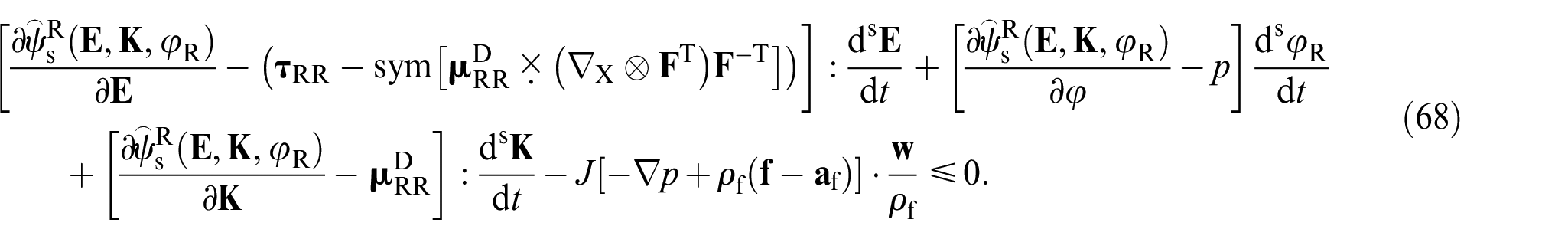
With the use of equations (62), (63), and (67), the inequality (59) becomes:

$$\begin{array}{c}[\frac{\partial {\stackrel{⌢}{\psi }}_{\mathrm{s}}^{\mathrm{R}}(\mathbf{E},\mathbf{K},{\phi }_{\mathrm{R}})}{\partial \mathbf{E}}-({\mathbf{\tau }}_{\mathrm{RR}}-\mathrm{sym}\left[{\mathbf{\mu }}_{\mathrm{RR}}^{\mathrm{D}}\stackrel{\times }{·}({\nabla }_{\mathrm{X}}\otimes {\mathbf{F}}^{\mathrm{T}}){\mathbf{F}}^{-\mathrm{T}}\right])]:\frac{{\mathrm{d}}^{\mathrm{s}}\mathbf{E}}{\mathrm{d}t}+[\frac{\partial {\stackrel{⌢}{\psi }}_{\mathrm{s}}^{\mathrm{R}}(\mathbf{E},\mathbf{K},{\phi }_{\mathrm{R}})}{\partial \phi }-p]\frac{{\mathrm{d}}^{\mathrm{s}}{\phi }_{\mathrm{R}}}{\mathrm{d}t}\hfill \\ +[\frac{\partial {\stackrel{⌢}{\psi }}_{\mathrm{s}}^{\mathrm{R}}(\mathbf{E},\mathbf{K},{\phi }_{\mathrm{R}})}{\partial \mathbf{K}}-{\mathbf{\mu }}_{\mathrm{RR}}^{\mathrm{D}}]:\frac{{\mathrm{d}}^{\mathrm{s}}\mathbf{K}}{\mathrm{d}t}-J[-\nabla p+{\rho }_{\mathrm{f}}(\mathbf{f}-{\mathbf{a}}_{\mathrm{f}})]·\frac{\mathbf{w}}{{\rho }_{\mathrm{f}}}\le 0.\hfill \end{array}$$

(68)

Since inequality (68) is hold for all motions, we obtain the constitutive equations of the form:

$${\mathbf{\tau }}_{\mathrm{RR}}=\frac{\partial {\stackrel{⌢}{\psi }}_{\mathrm{s}}^{\mathrm{R}}(\mathbf{E},\mathbf{K},{\phi }_{\mathrm{R}})}{\partial \mathbf{E}}+\mathrm{sym}\left[{\mathbf{\mu }}_{\mathrm{RR}}^{\mathrm{D}}\stackrel{\times }{·}({\nabla }_{\mathrm{X}}\otimes {\mathbf{F}}^{\mathrm{T}}){\mathbf{F}}^{-\mathrm{T}}\right],$$

(69)

$${\mathbf{\mu }}_{\mathrm{RR}}^{\mathrm{D}}=\frac{\partial {\stackrel{⌢}{\psi }}_{\mathrm{s}}^{\mathrm{R}}(\mathbf{E},\mathbf{K},{\phi }_{\mathrm{R}})}{\partial \mathbf{K}},$$

(70)

$$p=\frac{\partial {\stackrel{⌢}{\psi }}_{\mathrm{s}}^{\mathrm{R}}(\mathbf{E},\mathbf{K},{\phi }_{\mathrm{R}})}{\partial {\phi }_{\mathrm{R}}},$$

(71)

and the dissipation inequality:

$$\mathcal{D}\equiv [-\nabla p+{\rho }_{\mathrm{f}}(\mathbf{f}-{\mathbf{a}}_{\mathrm{f}})]·\frac{\mathbf{w}}{{\rho }_{\mathrm{f}}}\ge 0,$$

(72)

where $\mathcal{D}$ represents the dissipation, per unit current volume, which is non-negative and associated with the viscous flow of the fluid through the porous skeleton.

5.3. Darcy’s law

Dissipation $\mathcal{D}$ is the scalar product of two power-conjugate vectors: the filtration vector $\mathbf{q}\equiv \mathbf{w}/{\rho }_{\mathrm{f}}$ and the corresponding driving force, i.e., the expression within brackets in equation (72). The simplest relation between them is Darcy’s law and, within the context of isotropic case, Darcy’s law takes the form:

$$\mathbf{q}=\frac{\kappa }{\eta }[-\nabla p+{\rho }_{\mathrm{f}}(\mathbf{f}-{\mathbf{a}}_{\mathrm{f}})],$$

(73)

where $\eta$ denotes the fluid viscosity and $\kappa$ denotes the permeability of the fluid. $\kappa$ is generally porosity dependent and can be determined by (e.g., Coussy [20]):

$$\kappa \left(\varphi \right)={\ell }^2\frac{{\varphi }^3}{1-{\varphi }^2},$$

(74)

with $\ell$ being the characteristic length associated with the geometry of the porous network.

6. Isotropic linear theory

We now restrict our attention to linear couple-stress theory of poroelasticity. In the linear theory, the deformation is small such that:

$$|{\mathbf{u}}_{\mathrm{s}}\otimes {\nabla }_{\mathrm{X}}|<<1,$$

(75)

$$\left|\frac{{\varphi }_{\mathrm{R}}-{\varphi }_0}{{\varphi }_0}\right|<<1,$$

(76)

$$\left|\frac{{\rho }_{\mathrm{s}}-{\rho }_{\mathrm{s}}^0}{{\rho }_{\mathrm{s}}^0}\right|<<1,$$

(77)

$$\left|\frac{{\rho }_{\mathrm{f}}-{\rho }_{\mathrm{f}}^0}{{\rho }_{\mathrm{f}}^0}\right|<<1,$$

(78)

where ${\mathbf{u}}_{\mathrm{s}}(\mathbf{X},t)\equiv \mathbf{\chi }(\mathbf{X},t)-\mathbf{X}$ denotes the solid displacement; ${\rho }_{\mathrm{s}}^0$ and ${\rho }_{\mathrm{f}}^0$ denote the initial densities of the solid and the fluid.

As a consequence of equation (75),

$$\mathbf{F}=\mathbf{I}+{\mathbf{u}}_{\mathrm{s}}\otimes {\nabla }_{\mathrm{X}}\approx \mathbf{I}.$$

(79)

Then

$$\nabla \approx {\nabla }_{\mathrm{X}},\mathbf{E}\approx \mathbf{\epsilon },\mathbf{K}\approx \mathbf{\chi },$$

(80)

where $\mathbf{\epsilon }$ and $\mathbf{\chi }$ denote the infinitesimal strain and the curvature tensor. They are defined by:

$$\mathbf{\epsilon }\equiv \frac{1}{2}(\nabla \otimes {\mathbf{u}}_{\mathrm{s}}+{\mathbf{u}}_{\mathrm{s}}\otimes \nabla ),$$

(81)

$$\mathbf{\chi }\equiv \nabla \times \mathbf{\epsilon }=\frac{1}{2}(\nabla \times {\mathbf{u}}_{\mathrm{s}})\otimes \nabla .$$

(82)

Thus, by equations (79)–(82), constitutive equations (69)–(71) become:

$$\mathbf{\tau }=\frac{\partial {\hat{W}}_{\mathrm{s}}(\mathbf{\epsilon },\mathbf{\chi },{\phi }_{\mathrm{R}})}{\partial \mathbf{\epsilon }}+\mathrm{sym}\left[{\mathbf{\mu }}^{\mathrm{D}}\stackrel{\times }{·}(\nabla \otimes \nabla \otimes \mathbf{u})\right],$$

(83)

$${\mathbf{\mu }}^{\mathrm{D}}=\frac{\partial {\hat{W}}_{\mathrm{s}}(\mathbf{\epsilon },\mathbf{\chi },{\phi }_{\mathrm{R}})}{\partial \mathbf{\chi }},$$

(84)

$$p=\frac{\partial {\hat{W}}_{\mathrm{s}}(\mathbf{\epsilon },\mathbf{\chi },{\phi }_{\mathrm{R}})}{\partial {\phi }_{\mathrm{R}}},$$

(85)

with $W_{\mathrm{s}}={\hat{W}}_{\mathrm{s}}(\mathbf{\epsilon },\mathbf{\chi },{\phi }_{\mathrm{R}})$ denoting the free energy of the solid skeleton. Furthermore, it follows from equation (75) that:

$$\left|\frac{\partial {\hat{W}}_{\mathrm{s}}(\mathbf{\epsilon },\mathbf{\chi },{\phi }_{\mathrm{R}})}{\partial \mathbf{\chi }}\stackrel{\times }{·}(\nabla \otimes \nabla \otimes \mathbf{u})\right|<<\left|\frac{\partial {\hat{W}}_{\mathrm{s}}(\mathbf{\epsilon },\mathbf{\chi },{\phi }_{\mathrm{R}})}{\partial \mathbf{\epsilon }}\right|,$$

(86)

and hence equation (83) simplifies to:

$$\mathbf{\tau }=\frac{\partial {\hat{W}}_{\mathrm{s}}(\mathbf{\epsilon },\mathbf{\chi },{\phi }_{\mathrm{R}})}{\partial \mathbf{\epsilon }}.$$

(87)

Equations (84), (85), and (87) are the constitutive equations for the theory of poroelasticity with couple-stress at infinitesimal strains.

For an isotopic linear solid skeleton, $W_{\mathrm{s}}$ has the specific form:

$$W_{\mathrm{s}}=\frac{1}{2}\lambda {\left(\mathrm{tr}\mathbf{\epsilon }\right)}^2+\frac{1}{2}N{({\phi }_{\mathrm{R}}-b\mathrm{tr}\mathbf{\epsilon })}^2+\mu \mathbf{\epsilon }:\mathbf{\epsilon }+2\eta \mathbf{\chi }:\mathbf{\chi }+2\eta \prime \mathbf{\chi }:{\mathbf{\chi }}^{\mathrm{T}},$$

(88)

where $\lambda$ , $\mu$ , $b$ , and $N$ are the poroelastic moduli as in the linear poroelasticity, and $\eta$ and $\eta \prime$ are the two extra constitutive moduli introduced in the couple-stress theory (In fact, $\eta \prime$ does not appear in the equations of motion (104).). Specifically, $\lambda$ and $\mu$ are the Lamé moduli, and they are determined by:

$$\lambda =K-\frac{2}{3}G,\mu =G,$$

(89)

with $K$ and $G$ being the drained bulk modulus and the shear modulus; the Biot coefficient $b$ and the constant $N$ are given by:

$$b=1-\frac{K}{K_{\mathrm{s}}},\frac{1}{N}=\frac{b-{\varphi }_0}{K_{\mathrm{s}}},$$

(90)

with $K_{\mathrm{s}}$ being the bulk modulus of the solid phase/grains. Furthermore, the positive definite of $W_{\mathrm{s}}$ requires:

$$\mu >0,\lambda +\frac{2}{3}\mu >0,N>0,\eta >0,-1<\eta \prime /\eta <1.$$

(91)

Finally, from equations (84), (85), and (87), we obtain:

$$\mathbf{\tau }=(\lambda \mathrm{tr}\mathbf{\epsilon }-\mathrm{bp})\mathbf{I}+2\mu \mathbf{\epsilon },$$

(92)

$$p=N({\phi }_{\mathrm{R}}-b\mathrm{tr}\mathbf{\epsilon }),$$

(93)

$${\mathbf{\mu }}^{\mathrm{D}}=4(\eta \mathbf{\chi }+\eta \prime {\mathbf{\chi }}^{\mathrm{T}}).$$

(94)

In addition, if the couple-stress $\mathbf{\mu }$ is assumed symmetric, $W_{\mathrm{s}}$ should have the form:

$$W_{\mathrm{s}}=\frac{1}{2}\lambda {\left(\mathrm{tr}\mathbf{\epsilon }\right)}^2+\frac{1}{2}N{({\phi }_{\mathrm{R}}-b\mathrm{tr}\mathbf{\epsilon })}^2+\mu \mathbf{\epsilon }:\mathbf{\epsilon }+2\stackrel{⌢}{\eta }\stackrel{⌢}{\mathbf{\chi }}:\stackrel{⌢}{\mathbf{\chi }},$$

(95)

with the symmetric curvature tensor $\stackrel{⌢}{\mathbf{\chi }}$ defined by:

$$\stackrel{⌢}{\mathbf{\chi }}\equiv \frac{1}{2}(\mathbf{\chi }+{\mathbf{\chi }}^{\mathrm{T}})=\frac{1}{2}(\nabla \times \mathbf{\epsilon }-\mathbf{\epsilon }\times \nabla ),$$

(96)

and equation (94) should be replaced by:

$${\mathbf{\mu }}^{\mathrm{D}}=4\stackrel{⌢}{\eta }\stackrel{⌢}{\mathbf{\chi }}.$$

(97)

This is the so-called modified couple-stress theory, originally proposed by Yang et al. [19] (see also Hadjesfandiari and Dargush [24], Neff et al. [25], and Münch et al. [26]). The crucial advantage of the model is that only one extra constitutive modulus, namely, $\stackrel{⌢}{\eta }$ $(\stackrel{⌢}{\eta }>0)$ , needs to be introduced. However, because of the difficulties involved in seeking the Lagrangian couple-stress (symmetric) work-conjugate to:

$$\stackrel{⌢}{\mathbf{K}}\equiv \frac{1}{2}(\mathbf{K}+{\mathbf{K}}^{\mathrm{T}})=\frac{1}{2}({\nabla }_{\mathrm{X}}\times \mathbf{E}-\mathbf{E}\times {\nabla }_{\mathrm{X}}),$$

(98)

we, for consistency, disregard the foregoing assumption.

Furthermore, the linear behavior of saturating fluid requires the tangent bulk modulus $K_{\mathrm{f}}$ in equation (45) be a constant.

7. Boundary conditions

The field equations (26) and (73) need to be supplemented by appropriate boundary conditions. These conditions include the mechanical boundary conditions and the hydraulic boundary conditions.

The mechanical conditions involve either the force-stress vector, the tangent components of the couple-stress vector or the displacement, the tangent components of the rotation vector ${\mathbf{\theta }}_{\mathrm{s}}$ ( ${\mathbf{\theta }}_{\mathrm{s}}\equiv 1/2\nabla \times {\mathbf{u}}_{\mathrm{s}}$ ); they are:

$$\mathit{\tau }\mathbf{n}+\frac{1}{2}\mathbf{n}\times [{\mathbf{\mu }}^{\mathrm{D}}·\nabla -\nabla {\mu }_{\mathrm{nn}}^{\mathrm{D}}]={\overline{\mathbf{t}}}_n,\mathrm{or}{\mathbf{u}}_{\mathrm{s}}={\overline{\mathbf{u}}}_{\mathrm{s}},$$

(99)

$$(\mathbf{I}-\mathbf{n}\otimes \mathbf{n})\left(\mathbf{\mu }\mathbf{n}\right)={\overline{\mathbf{m}}}_n^t,\mathrm{or}(\mathbf{I}-\mathbf{n}\otimes \mathbf{n}){\mathbf{\theta }}_{\mathrm{s}}={\overline{\mathbf{\theta }}}_{\mathrm{s}}^t,$$

(100)

where

$${\mu }_{\mathrm{nn}}^{\mathrm{D}}=\mathbf{n}·\left({\mathbf{\mu }}^{\mathrm{D}}\mathbf{n}\right),$$

(101)

and ${\overline{\mathbf{t}}}_n$ , ${\overline{\mathbf{m}}}_n^t$ , ${\overline{\mathbf{u}}}_{\mathrm{s}}$ , and ${\overline{\mathbf{\theta }}}_{\mathrm{s}}^t$ are the prescribed surface force-stress traction, tangent components of surface couple-stress traction, surface displacement, and tangent components of surface rotation. Note that only five independent mechanical conditions need to be prescribed on the boundary as concluded by Mindlin and Tiersten [17] and Koiter [18].

Furthermore, if the boundary surface is piecewise smooth and has an edge $C$ , formed by the intersection of two bounding surface, the edge condition:

$$\mathrm{\Delta }\left({\mu }_{\mathrm{nn}}^{\mathrm{D}}\right)={\overline{t}}_c,\mathrm{or}{\mathbf{u}}_{\mathrm{s}}·\mathbf{k}={\overline{u}}_{\mathrm{s}}^k,$$

(102)

on $C$ must be added to the conditions (99) and (100). Here, $\mathrm{\Delta }({\mu }_{\mathrm{nn}}^{\mathrm{D}})$ denotes the jump in value $\mathrm{\Delta }$ of $({\mu }_{\mathrm{nn}}^{\mathrm{D}})$ on each side of $C$ ; ${\overline{t}}_c$ denotes the prescribed line force (per unit length), tangent to the edge; ${\overline{u}}_{\mathrm{s}}^k$ denotes the prescribed displacement, tangent to the edge; $\mathbf{k}$ is the unit vector tangent to the edge $C$ .

The hydraulic conditions involve either the fluid pressure or the fluid flux; they are:

$$p=\overline{p},\mathrm{or}\mathbf{q}·\mathbf{n}={\overline{q}}_n,$$

(103)

where $\overline{p}$ and ${\overline{q}}_n$ are the prescribed surface fluid pressure and normal component of surface fluid flux.

8. Examples

As an example, we consider application of the couple-stress–based strain-gradient theory to the wave propagation in fluid-saturated porous solids. In the absence of the body force, the equation of motion (26) and Darcy’s law (73) can be reformulated with displacements as:

$$\mu {\nabla }^2{\mathbf{u}}_{\mathrm{s}}+(\lambda +\mu )\nabla \nabla ·{\mathbf{u}}_{\mathrm{s}}+\mu l^2{\nabla }^2\nabla \times \nabla \times {\mathbf{u}}_{\mathrm{s}}-b\nabla p={\rho }_0^{\mathrm{s}}(1-{\varphi }_0)\frac{{\partial }^2{\mathbf{u}}_{\mathrm{s}}}{\partial t^2}+{\rho }_0^{\mathrm{f}}{\varphi }_0\frac{{\partial }^2{\mathbf{u}}_{\mathrm{f}}}{\partial t^2},$$

(104)

$$\nabla p+\frac{\eta }{\kappa }{\varphi }_0(\frac{\partial {\mathbf{u}}_{\mathrm{f}}}{\partial t}-\frac{\partial {\mathbf{u}}_{\mathrm{s}}}{\partial t})=-{\rho }_0^{\mathrm{f}}\frac{{\partial }^2{\mathbf{u}}_{\mathrm{f}}}{\partial t^2},$$

(105)

where use has been made of equations (81), (82), (92), and (94), and ${\mathbf{u}}_{\mathrm{s}}$ and ${\mathbf{u}}_{\mathrm{f}}$ denote, respectively, the solid and fluid displacements. Here, the material length $l$ is defined by:

$$l=\sqrt{\frac{\eta }{\mu }},$$

(106)

which is microstructure dependent. Its effect on the responses of the material should be important at small-length scales. For $l=0$ , equation (104) reduces to the conventional equation of motion as in the theory of poroelasticity. Note that the constant $\eta \prime$ does not appear in equation (104).

Next, differentiating equation (93) and using equation (44) yields:

$$\frac{\mathrm{d}{m}_{\mathrm{f}}}{{\rho }_{\mathrm{f}}}=b\mathrm{d}\left(\mathrm{tr}\mathbf{\epsilon }\right)+\frac{1}{M}\mathrm{d}p,$$

(107)

with the modulus $M$ defined as:

$$\frac{1}{M}=\frac{1}{N}+\frac{{\varphi }_0}{K_{\mathrm{f}}}.$$

(108)

Integrating equation (107) under condition (78) gives:

$$\frac{m_{\mathrm{f}}-m_{\mathrm{f}}^0}{{\rho }_{\mathrm{f}}^0}=b\mathrm{tr}\mathbf{\epsilon }+\frac{1}{M}p,$$

(109)

with $m_{\mathrm{f}}^0$ being the initial fluid mass content. Differentiating equation (109) with respect to time, one has:

$$\frac{1}{{\rho }_{\mathrm{f}}^0}\frac{\partial m_{\mathrm{f}}}{\partial t}=b\frac{\partial }{\partial t}\left(\mathrm{tr}\mathbf{\epsilon }\right)+\frac{1}{M}\frac{\partial p}{\partial t}.$$

(110)

Then, combining equation (110) with mass conservation equation of pore fluid at small deformations, i.e.,

$$\frac{\partial m_{\mathrm{f}}}{\partial t}+\nabla ·\mathbf{w}=0,$$

(111)

we have:

$$\frac{\partial p}{\partial t}=-M\frac{\partial }{\partial t}[(b-{\varphi }_0)\nabla ·{\mathbf{u}}_{\mathrm{s}}+{\varphi }_0\nabla ·{\mathbf{u}}_{\mathrm{f}}].$$

(112)

Equation (112) severs the purpose of reformulating equations (104) and (105) in terms of displacements in the frequency domain.

For harmonic wave motions, we consider:

$${\mathbf{u}}_{\mathrm{s}}(\mathbf{x},t)={\tilde{\mathbf{u}}}_{\mathrm{s}}\left(\mathbf{x}\right)\exp (-i\omega t),$$

(113)

$${\mathbf{u}}_{\mathrm{f}}(\mathbf{x},t)={\tilde{\mathbf{u}}}_{\mathrm{f}}\left(\mathbf{x}\right)\exp (-i\omega t),$$

(114)

$$p(\mathbf{x},t)=\tilde{p}\left(\mathbf{x}\right)\exp (-i\omega t),$$

(115)

where ${\tilde{\mathbf{u}}}_{\mathrm{s}}$ , ${\tilde{\mathbf{u}}}_{\mathrm{f}}$ , and $\tilde{p}$ , with a superposed hat, are the amplitudes, and $\omega$ is the circular frequency. For the simplicity of notation, the superposed hat will be omitted in the subsequent analysis.

Substituting equations (113)–(115) into equations (104) and (105) with use of equation (112), we obtain:

$$\mu {\nabla }^2{\mathbf{u}}_{\mathrm{s}}+(\lambda +\mu -\mathrm{bM}({\varphi }_0-b))\nabla \nabla ·{\mathbf{u}}_{\mathrm{s}}+{\varphi }_0\mathrm{bM}\nabla \nabla ·{\mathbf{u}}_{\mathrm{f}}+\mu l^2{\nabla }^2\nabla \times \nabla \times {\mathbf{u}}_{\mathrm{s}}=-{\omega }^2({\rho }_0^{\mathrm{s}}(1-{\varphi }_0){\mathbf{u}}_{\mathrm{s}}+{\rho }_0^{\mathrm{f}}{\varphi }_0{\mathbf{u}}_{\mathrm{f}}).$$

(116)

$$M[(b-{\varphi }_0)\nabla \nabla ·{\mathbf{u}}_{\mathrm{s}}+{\varphi }_0\nabla \nabla ·{\mathbf{u}}_{\mathrm{f}}]-i\omega \frac{\eta }{\kappa }{\varphi }_0{\mathbf{u}}_{\mathrm{s}}=-{\omega }^2({\rho }_0^{\mathrm{f}}+\frac{i}{\omega }\frac{\eta }{\kappa }{\varphi }_0){\mathbf{u}}_{\mathrm{f}}.$$

(117)

We now consider the Helmholtz resolutions:

$${\mathbf{u}}_{\mathrm{s}}=\nabla {\phi }_{\mathrm{s}}+\nabla \times {\mathbf{H}}_{\mathrm{s}},\nabla ·{\mathbf{H}}_{\mathrm{s}}=0,$$

(118)

$${\mathbf{u}}_{\mathrm{f}}=\nabla {\phi }_{\mathrm{f}}+\nabla \times {\mathbf{H}}_{\mathrm{f}},\nabla ·{\mathbf{H}}_{\mathrm{f}}=0,$$

(119)

where ${\phi }_{\mathrm{s}}$ and ${\phi }_{\mathrm{f}}$ are the scalar potentials and ${\mathbf{H}}_{\mathrm{s}}$ and ${\mathbf{H}}_{\mathrm{f}}$ are the zero-divergence vector potentials. The motions associated with ${\phi }_{\mathrm{s}}$ and ${\phi }_{\mathrm{f}}$ are dilatational and those with ${\mathbf{H}}_{\mathrm{s}}$ and ${\mathbf{H}}_{\mathrm{f}}$ are rotational.

Introducing equations (118) and (119) into equations (116) and (117) yields:

$$[\lambda +2\mu -\mathrm{bM}({\varphi }_0-b)]{\nabla }^2{\phi }_{\mathrm{s}}+{\varphi }_0\mathrm{bM}{\nabla }^2{\phi }_{\mathrm{f}}+{\omega }^2{\rho }_0^{\mathrm{s}}(1-{\varphi }_0){\phi }_{\mathrm{s}}+{\omega }^2{\rho }_0^{\mathrm{f}}{\varphi }_0{\phi }_{\mathrm{f}}=0,$$

(120)

$$M(b-{\varphi }_0){\nabla }^2{\phi }_{\mathrm{s}}+{\varphi }_{0}M{\nabla }^2{\phi }_{\mathrm{f}}-i\omega \frac{\eta }{\kappa }{\varphi }_0{\phi }_{\mathrm{s}}+{\omega }^2({\rho }_0^{\mathrm{f}}+\frac{i}{\omega }\frac{\eta }{\kappa }{\varphi }_0){\phi }_{\mathrm{f}}=0,$$

(121)

$$\mu (1-l^2{\nabla }^2){\nabla }^2{\mathbf{H}}_{\mathrm{s}}+{\omega }^2{\rho }_0^{\mathrm{s}}(1-{\varphi }_0){\mathbf{H}}_{\mathrm{s}}+{\omega }^2{\rho }_0^{\mathrm{f}}{\varphi }_0{\mathbf{H}}_{\mathrm{f}}=0,$$

(122)

$$-i\omega \frac{\eta }{\kappa }{\varphi }_0{\mathbf{H}}_{\mathrm{s}}+{\omega }^2({\rho }_0^{\mathrm{f}}+\frac{i}{\omega }\frac{\eta }{\kappa }{\varphi }_0){\mathbf{H}}_{\mathrm{f}}=0,$$

(123)

The first two equations (120) and (121) are same as those obtained in the conventional poroelasticity and, from equations (120) and (121), we obtain the dispersion relation (refer to Zheng and Ding [27] for more details):

$$k_{P1,2}\left(\omega \right)=\omega \sqrt{x_{1,2}},$$

(124)

where

$$x_{1,2}=\frac{-b\mp \sqrt{b^2-4\mathrm{ac}}}{2a},$$

(125)

with:

$$a=(\lambda +2\mu ){\varphi }_{0}M,b=-(\lambda +2\mu +b^{2}M)({\rho }_0^{\mathrm{f}}+\frac{i}{\omega }\frac{\eta }{\kappa }{\varphi }_0)+{\varphi }_{0}M(2b{\rho }_0^{\mathrm{f}}-{\rho }_0),$$

(126)

$$c={\rho }_0^{\mathrm{f}}[(1-{\varphi }_0){\rho }_0^{\mathrm{s}}+\frac{i}{\omega }\frac{\eta }{\kappa }{\varphi }_0],{\rho }_0={\rho }_0^{\mathrm{s}}(1-{\varphi }_0)+{\rho }_0^{\mathrm{f}}{\varphi }_0,$$

(127)

here, $k_{P1,2}$ are the complex wavenumbers of the fast (P1) and slow (P2) compressional waves. Note that, for the time dependence of the form $\exp (-i\omega t)$ , the choice of square root of $x_{1,2}$ should meet the requirement that the resulting wavenumber has both positive real and imaginary parts (which lead to a positive phase velocity and a decrease in wave amplitudes) and that, this principle is also applied to the determination of the wavenumber of rotational waves.

Furthermore, the phase velocities $v_{P1,2}$ are determined by:

$$v_{P1,2}=\frac{\omega }{\mathrm{Re}\left(k_{P1,2}\right)}.$$

(128)

For rotational waves, combining equation (122) with equation (123) gives:

$$(l^2{\nabla }^2-1){\nabla }^2{\mathbf{H}}_{\mathrm{s}}-{\omega }^2\frac{\hat{\rho }}{\mu }{\mathbf{H}}_{\mathrm{s}}=0,$$

(129)

with $\hat{\rho }$ defined by:

$$\hat{\rho }\equiv (1-{\varphi }_0){\rho }_0^{\mathrm{s}}+\frac{1}{1-i\omega \frac{\kappa }{\eta }\frac{{\rho }_0^{\mathrm{f}}}{{\varphi }_0}}{\rho }_0^{\mathrm{f}}{\varphi }_0.$$

(130)

From equation (129), we derive the dispersion relation:

$$k_S\left(\omega \right)=\sqrt{y},$$

(131)

with:

$$y=\frac{1}{2l^2}(-1+\sqrt{1+4{\omega }^2{l}^2\frac{\hat{\rho }}{\mu }}).$$

(132)

Note that $y=(-1-\sqrt{1+4{\omega }^2{l}^2\hat{\rho }/\mu })/2l^2$ has been neglected since its two square roots violate the requirement that both real and imaginary parts of wavenumbers should be positive as mentioned before.

The phase velocities $v_S$ of rotational waves are given by:

$$v_S=\frac{\omega }{\mathrm{Re}\left(k_S\right)}.$$

(133)

For $l=0$ , equation (131) reduces to:

$$k_S\left(\omega \right)=\omega \sqrt{\frac{\hat{\rho }}{\mu }},$$

(134)

which is the complex wave numbers of rotational waves predicted by the conventional poroelasticity.

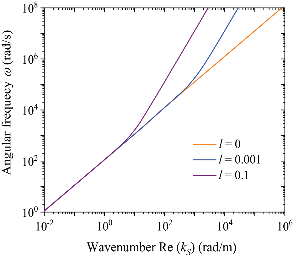
Plots of $\omega$ as functions of $\mathrm{Re}(k_S)$ for $l=0$ , $l=0.001$ , $l=0.1$ are provided in Figure 1. Note that $l=0$ corresponds to the case in which the gradient effects are absent. It is observed that $\omega$ increases with $\mathrm{Re}(k_S)$ and this trend is enhanced by increasing $l$ , which indicates the stiffness enhancement is present as the curl of the strain is taken into account. Furthermore, this enhancement is only observable at higher frequencies. Similar observations have been made in strain-gradient elastic materials (e.g., Lim et al. [28]).

Figure 1.

Dispersion curves of rotational waves. The material parameters used for the calculation are $\mu =24.9\mathrm{MPa}$ , ${\varphi }_0=0.408$ , ${\rho }_0^{\mathrm{s}}=2650\mathrm{kg}/{\mathrm{m}}^3$ , ${\rho }_0^{\mathrm{f}}=1000\mathrm{kg}/{\mathrm{m}}^3$ , $\kappa =1.0\times {10}^{-10}{\mathrm{m}}^2$ , and $\eta =1.0\times {10}^{-3}\mathrm{Pa}\mathrm{s}$ .

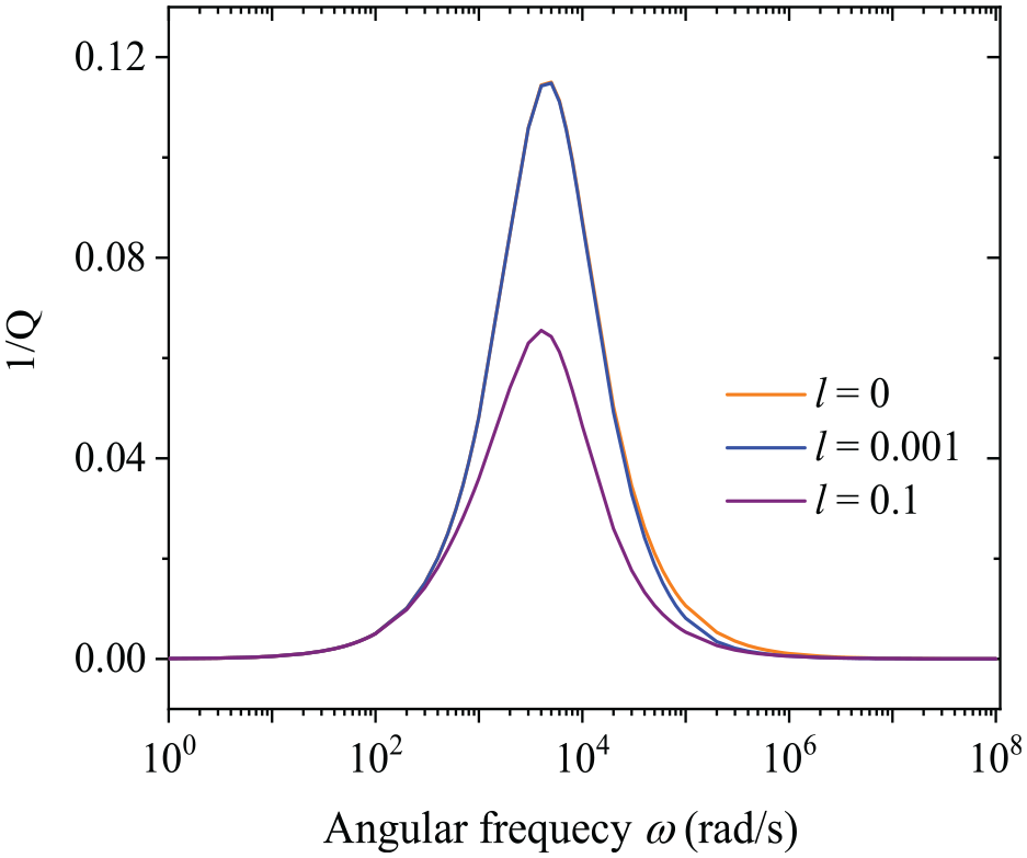
Both wave dispersion and attenuation occur in fluid-saturated materials. To measure the attenuation loss, a dimensionless quantity $Q$ (the quality factor), expressed by Mavko et al. [29]:

$$\frac{1}{Q}\approx 2\frac{\mathrm{Im}(k_S)}{\mathrm{Re}(k_S)},$$

(135)

is introduced. Note that $1/Q$ measures the fraction of energy dissipated in each wave period and the lower $Q$ , the larger the dissipation is. From Figure 2, it is noticed that the energy dissipation decreases with increasing $l$ and the curl of the strain has no effect on the critical frequency at which $1/Q$ attains a peak value (the maximum attenuation occurs).

Figure 2.

Attenuation curves of rotational waves.

Because the dispersion relation (124) for P1- and P2-waves is same as that in classical poroelasticity, the curl of the strain has no effect on the dispersion and attenuation of compressional waves. Hence, examples are no longer provided for illustration.

9. Concluding remarks

In this paper, we proposed a couple-stress–based gradient theory for fluid-saturated porous solids by including the solid vorticity gradient. We developed the theory within the finite deformation framework and, subsequently, derived a linearized theory for an isotropic porous solid in which two microstructure-dependent constitutive moduli (or equivalently, two material length-scale parameters) were introduced. Note that only one of them appears in the equation of motion and, nevertheless, the other may enter the displacement of solid through certain of the mechanical boundary conditions. By assuming the couple-stress being symmetric, the theory will be simplified in the sense that only one material length-scale parameter needs to be involved.

In the proposed theory, the solid vorticity gradient ${\mathbf{\omega }}_{\mathrm{s}}\otimes \nabla$ is included to account for the microstructure effects, whereas high-order gradient terms of the saturating fluid are excluded. Consequently, the resulting force-stress in fluid is spherical and Darcy’s law takes the same form as that in the conventional theory, which is a key feature of the model. Nevertheless, if the fluid free energy is allowed to be dependent on density gradient, their respective forms, which are constitutive dependent, need to be modified. The other consequence of presence of fluid density gradient is that the solid free energy ${\stackrel{⌢}{\psi }}_{\mathrm{s}}^{\mathrm{R}}$ is dependent on the gradient of Lagrangian porosity change ${\nabla }_{\mathrm{X}}{\phi }_{\mathrm{R}}$ (refer to equation (56)) due to the presence of solid–fluid coupling in the material.