We first show that the minimization problem associated with the nonlinear shell model of W.T. Koiter becomes coercive over its natural space of admissible deformations when the third fundamental form is added to its functional. Then, under the assumption that the middle surface of the shell is a minimal surface, we approach this minimization problem by a new minimization problem that is well-posed over the same space of admissible deformations.
The nonlinear shell model of W.T. Koiter, so named after Koiter [1], is a system of nonlinear partial differential equations whose solution predicts the deformation of a nonlinearly elastic shell in response to applied forces and boundary conditions. In its classical formulation (see Koiter [1] or Ciarlet [2, section 11.1]), Koiter’s model applies to shells made of an elastic material that is homogeneous and isotropic, so that its behavior is modeled by two elastic coefficients, denoted and , via the two-dimensional elasticity tensor:
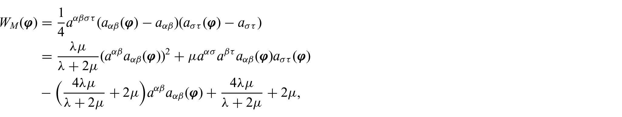
the membrane energy:
and the flexural energy:
associated with an admissible deformation of the middle surface of the shell. Note that the membrane energy is a measure of the change of metric tensor field associated with , while the flexural energy is a measure of the change of curvature tensor field associated with (cf. equation (10)).
Then, the system of partial differential equations constituting the nonlinear shell model of W.T. Koiter is the strong formulation of the Euler–Lagrange equation associated with the functional:
defined over the set of all admissible deformations of the middle surface of the shell, where:
and is a given function representing the potential of the applied forces.
By admissible deformation, we mean a smooth enough immersion satisfying the boundary conditions imposed on the shell. We assume that these boundary conditions are:
where is a non-empty relatively open subset of the boundary of . Note that this boundary condition is a consequence of Kirchhoff–Love assumption on the admissible deformations (see relation (13) in section 3), combined with the assumption that the shell is kept fixed at the points of its boundary for all and .
The functional (4) is neither coercive nor polyconvex (in the sense of Ball et al. [3] or Ciarlet et al. [4]). This is why existence theorems have been established in the literature not for the nonlinear shell model of W.T. Koiter itself, but for ad hoc approximations of Koiter’s model whereby the integrand in Koiter’s functional (4) is replaced by:
where the additional term is defined in such a way that is coercive, polyconvex, and negligible compared with .
Finding the best additional term remains an open question, however. Up to now, it has been done only in particular cases, or under additional assumptions on the shell, as follows: by Bunoiu et al. [5] for spherical shells, by Ciarlet and Mardare [6] for almost spherical shells, and by Anicic [7, 8] for deformations with principal radii of curvatures bounded below by . A different approach whereby is defined by averages across the thickness of specific three-dimensional densities was proposed by Ciarlet and Mardare [9] and Mardare [10].
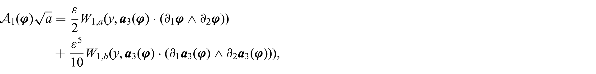
The objective of this paper is twofold: first, we show that should contain a term of the form:
where:
is a measure of change of the third fundamental form when the middle surface of the shell undergoes a deformation ; this will ensure that is coercive (section 3).
Second, we show how to define the remaining part of to ensure that the functional (4) with replaced by is also sequentially weaker lower semi-continuous and then establish existence theorems for the corresponding minimization problems. These existence theorems are established for shells whose middle surface is either a planar surface (section 5) or a non-planar minimal surface (section 6), two cases that were not covered by the literature cited above.
Note that the two types of shells studied in this paper are important not only from a theoretical viewpoint but also for practical applications. This is because a flexible shell stretched over a given frame will take the form of a minimal surface, so in particular they are useful in architectural designs.
2. Notation and definitions
Throughout this paper, the Greek indices and exponents range in the set , and Latin indices and exponents range in the set (unless when they are used for indexing sequences). The summation convention with respect to repeated indexes and exponents is used.
Strong and weak convergences in any normed vector space are respectively denoted
Vector and matrix fields are denoted by boldface letters. The Euclidean norm, the inner product, and the vector product of two vectors and in are, respectively, denoted , , and . Given any integers and , the inner product and the Frobenius norm in are, respectively, denoted and defined by and , where denote the trace operator of square matrices. The subspace of formed by all symmetric matrices is denoted . Notation such as , , or designates a matrix whose component at its -row and -column is , , or , respectively.
The notation denotes a generic point in and denotes the weak partial derivative operator with respect to .
Given any open subset of and any real number , the notation denotes the space of matrix fields with components in the Lebesgue space . It is equipped with the norm:
The notation denotes the space of vector fields with components in the Sobolev space . It is equipped with the norm:
where is the matrix field with at its row and column .
Throughout this paper, a surface in is given once and for all, where is a bounded Lipschitz domain and is an immersion of class such that the vector field , defined by:
is also of class . Note that is a unit vector normal to the surface at the point . The area element on the surface is , where:
The assumption that is a bounded Lipschitz domain means that is open, bounded, and connected, with a Lipschitz-continuous boundary in the sense of Adams and Fournier [11], so that lies locally on only one side of its boundary. Note that the assumption that the boundary of is Lipschitz-continuous boundary in the sense of Adams & Fournier means that each point on the boundary of should have a neighborhood whose intersection with the boundary of should be the graph of a Lipschitz-continuous function (cf. Adams and Fournier [11]).
The assumption that is an immersion of class means that and the two vector fields are linearly independent at every , so that the denominator in equation (7) does not vanish.
The covariant components of the first fundamental form of the surface are the functions:
and the contravariant components of the same form are the components of the inverse matrix:
Note that both matrices and are symmetric and positive definite at every .
The covariant components of the second and third fundamental forms of the surface are, respectively, the functions:
and
Note that the matrices are symmetric and non-negative-definite for all and that:
The mean curvature and the total curvature of the surface are the functions denoted and defined by:
and
where and are the principal curvatures of the surface at the point , defined as the eigenvalues of the matrix .
The operations of raising and lowering indices of tensor fields on are defined with respect to the metric (i.e., the first fundamental form) induced by the immersion , even when other immersions are defined over the same set . In particular:
are the mixed components of, respectively, the second and third fundamental forms of the surface , and:
are the contravariant components of respectively the second and third fundamental forms of the same surface.
The above definitions are generalized to surfaces with little regularity as follows. By surface with little regularity, we mean a subset defined as the image of a bounded Lipschitz domain by a function such that:
Such a function is also called immersion, even though the above relation holds only almost everywhere.
With every immersion , we associate the vector field:
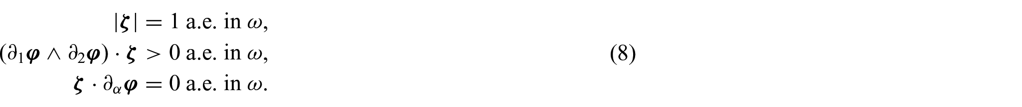
Note that is the unique unit vector field on that is positively oriented and normal to the surface at almost all points of . This means that is the unique vector field satisfying the following properties:
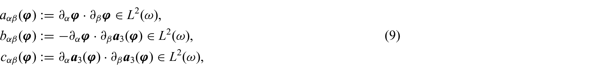
With every immersion such that , we associate the functions:
the functions:
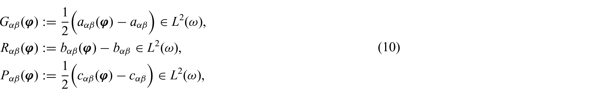
and the functions:
Note that is the area element on the surface with little regularity , that the functions defined by equation (9) are the covariant components of the fundamental forms (defined in a weaker sense) for the surface , and that the functions defined by equation (10) measure the difference between the fundamental forms of the “fixed” surface and the “generic” surface . These functions are the basis of the definition of both Koiter’s nonlinear shell model (section 1) and of its approximations defined in this paper (sections 3, 5, and 6).
In all that follows, by shell we mean a three-dimensional body whose natural state (i.e., a stress-free configuration of the body) is a “surface with positive thickness” in the three-dimensional Euclidean space. This means that a shell is a subset of of the form:
where:
and
for some given bounded Lipschitz domain , real number , and immersion of class with a unit normal vector field also of class .
The real number represents the half-thickness of the shell and represents the middle surface of the shell. The upper bound of is chosen sufficiently small compared with the diameter of , so that is itself an immersion of class from into (the existence of such small is proved in Ciarlet [12]).
3. A coercive approximation of Koiter’s nonlinear shell model for general shells
The nonlinear shell model of W.T. Koiter, so named after Koiter [1], is a system of nonlinear partial differential equations defined over , derived by a formal asymptotic analysis when from the equations of nonlinear elasticity defined over . This derivation is made under specific a priori assumptions on the shell and its admissible deformations, as follows.
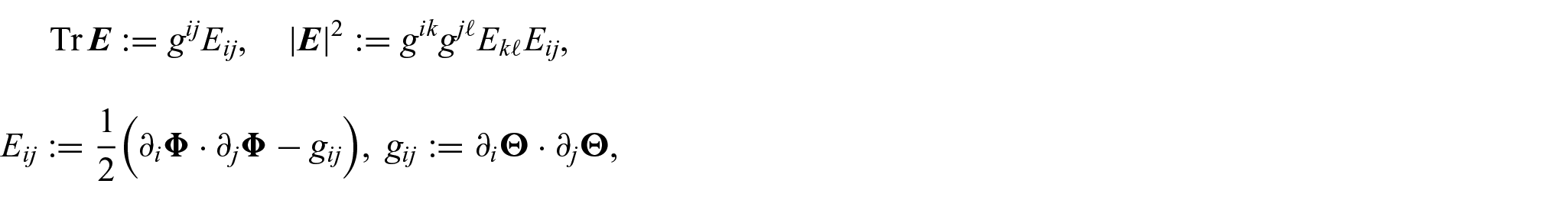
The first assumption is that the shell is made of a homogeneous and isotropic elastic material modeled by the constitutive law of Saint Venant–Kirchhoff. This means that the second Piola–Kirchhoff stress tensor field and the Green–St Venant strain tensor field associated with an admissible deformation of the shell are related to one another by the relation:
where and are the Lamé constants of the elastic material constituting the shell, denotes the trace operator, and denotes the identity tensor of order three.
Consequently, the equations of nonlinear elasticity modeling the shell are the strong formulation of the Euler–Lagrange equation associated with the functional:
representing the total energy of the shell, where is the potential of the applied forces:
are the components of the matrix field , and denote the partial differential operators in both classical and distributional sense, is the matrix field whose columns are the vector fields and , and:
denotes the volume element in the reference configuration of the shell. Note that are the covariant components of the tensor field with respect to the curvilinear coordinates defined by the global chart defining the reference configuration of the shell.
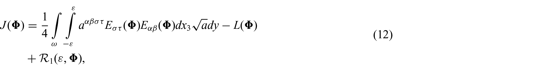
The second assumption is that the tensor field is planar and parallel to the middle surface of the shell. As proven in Mardare [13], this implies that the functional (11) can be written as:
where is negligible when compared with the double integral in equation (12).
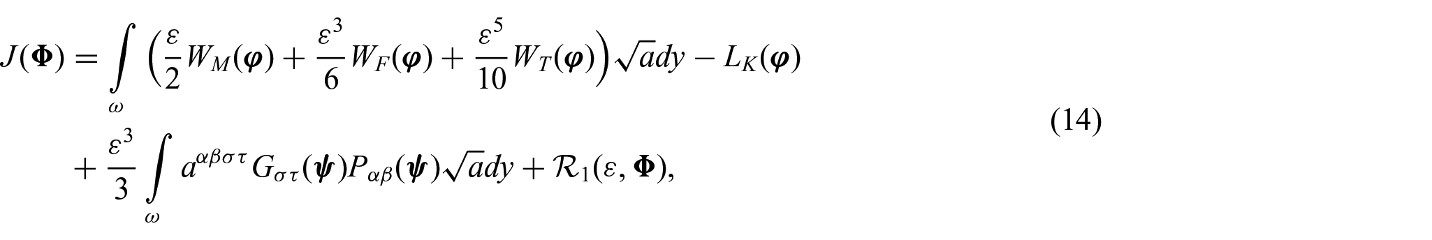
The third assumption is that the function appearing in functional (12) is of Kirchhoff–Love type, which means that:
for all and , where is a smooth enough immersion representing the deformation of the middle surface of the shell. Consequently, for each :
Note that Koiter’s functional (4) is obtained from the functional (14) simply by dropping from its first integral, its second integral altogether, and . This is justified for the strong formulation of Koiter’s model as a system of partial differential equations (see Koiter [1]), but not for the weak formulation of Koiter’s model as a minimization problem. The reason is that dropping from equation (14) leads to a loss of regularity of , which in turn implies that Koiter’s functional is not coercive in any meaningful way. To see this, note that Koiter’s functional is well-defined and finite if is an immersion of class such that , since then:
but equation (15) does not imply that . Indeed, consider, for instance, the immersion , defined by for all . Then, straightforward calculations show that and both belong to , while does not belong to .
By contrast, its approximation:
is well defined and finite if is an immersion of class such that , since then:
and, conversely, equation (17) implies that and . Indeed, the relations imply, in particular, that and , so that since is bounded. The same argument shows that the relations imply that .
Note that the functional is indeed an approximation of Koiter’s functional (defined by equation (4)) since the two functionals coincide at the first order for all sufficiently smooth immersions (cf. Lemma 1 in the next section). Note also that approaches the functional better than (cf. equation (14)).
Finally, the fourth assumption is that the deformations of the shell must preserve orientation and satisfy boundary conditions of clamping on the subset of its boundary, where:
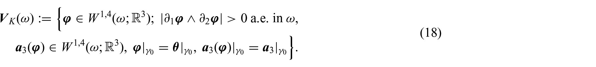
and is any non-empty relatively open subset of the boundary of . This implies that the admissible deformations of the shell are the elements of the set:
so that, in view of equation (13), the admissible deformations of the middle surface of the shell are the elements of the set:
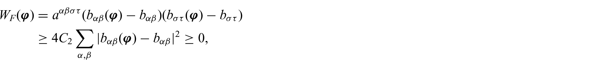
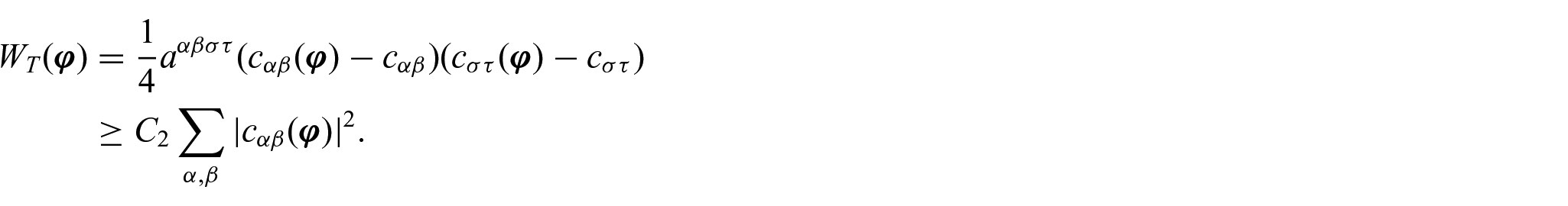
Note that the functionals and are both well-defined over , but only is coercive over this space. That is not coercive over is an immediate consequence of the observation made in the paragraph following formula (15). That is coercive over is an immediate consequence of the observation made in the paragraph following formula (17). Indeed, this latter observation implies that, for every in the dual of the space , one can find two constants and such that:
for all . This justifies keeping the third fundamental form, via , in the definition of the approximation of Koiter’s functional .
However, this is not enough to ensure the existence of a minimizer of over , since we do not know whether is sequentially weakly lower semi-continuous over or not.
We will overcome this difficulty in sections 5 and 6, using an argument similar to one used by Ciarlet and Geymonat [14] to overcome a similar difficulty in three-dimensional elasticity. The idea is to include in the definition of another negligible term that will make the new functional sequentially weakly lower semi-continuous, in addition to being coercive over the same space of admissible deformations as .
4. Preliminary lemmas
This section gathers all the preliminary results needed to define the sequentially weakly lower semi-continuous approximations of Koiter’s functional in sections 5 and 6, and then to prove that they possess minimizers in the set .
The first lemma shows that the functional is indeed an approximation of Koiter’s functional (defined by equation (4)).
Lemma 1.Given any immersion with that is sufficiently close in the -norm to the immersion , the following relations hold in :
Proof. We follow the proof of Lemma 2 in Bunoiu et al. [5].
Using Taylor’s expansion in power series of a matrix of type , where denotes the identity matrix of order two and is square matrix of order two such that , together with the definition of the functions , viz.,
we deduce that:
Besides, the definition of the functions implies that:
Then, the first estimate of the lemma is obtained using the two estimates above in the following expression of the functions :
The second relation of the lemma follows immediately from the first one and from the definition of the function , viz.,
The next four lemmas will be needed to establish existence theorems for the nonlinear shell models defined in both sections 5 and 6 (see the proofs of Theorems 2 and 4).
Lemma 2.Given any constants and , let:
for all functions such that:
Given any immersion that is sufficiently close in the -norm to the immersion , the following relation holds in :
Proof. We follow the proof of Lemma 1 in Bunoiu et al. [5].
The definition of the functions implies that:
Consequently,
on one hand.
On the other hand, Cayley–Hamilton theorem applied to the matrix field with components shows that:
where denotes the Kronecker symbol, so that (by applying the trace operator to it):
Then, we infer from the above relations that:
which in turn implies that:
The conclusion of the lemma follows using these relations in the definition of the function . □
Lemma 3.Given any constants and and any positive functions and , define the function by:
for all , and by:
Then:
whenever in when .
Proof. Since the functions and are positive and since for all , we have:
for all . Then, the function , defined by:
for all , satisfies:
Besides, is continuous and convex with respect to . Then, a classical theorem in the calculus of variations (see, for example, Dacorogna [15, Theorem 3.23]) shows that:
whenever in when .
In addition,
since in and (remember that is a bounded set by assumption).
Then, the conclusion follows by combining the last two relations. □
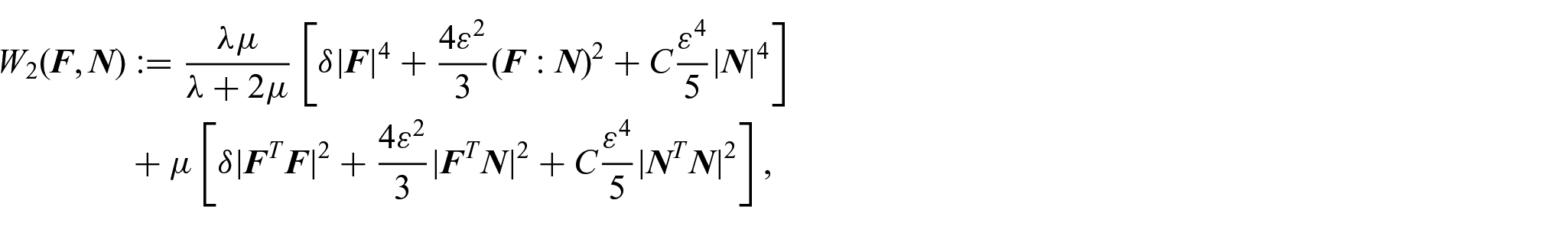
Lemma 4.Given any constants , , , and , let:
for all .
Assume that . Then:
whenever in when .
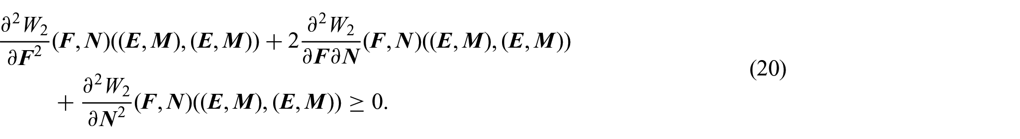
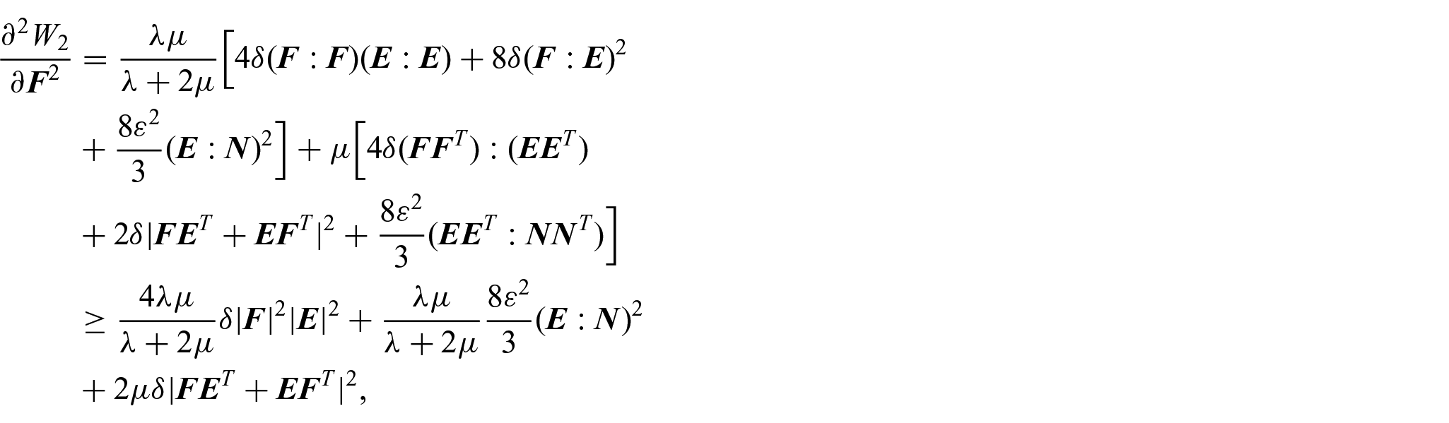
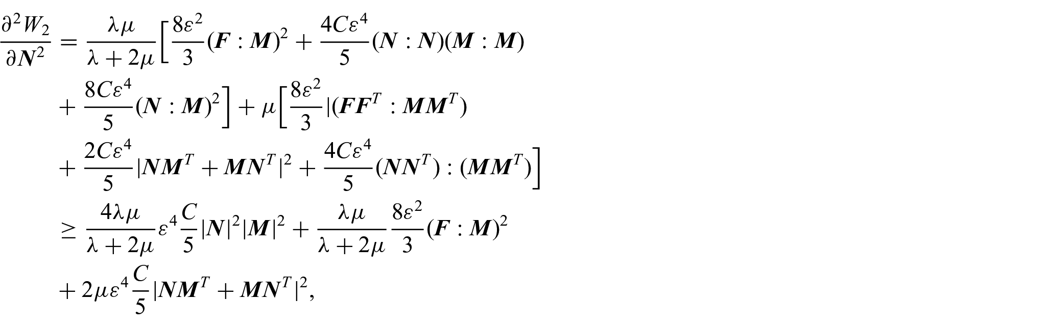
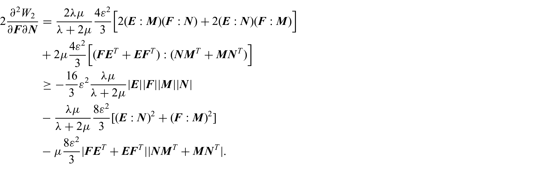
Proof. It suffices to prove that the function is convex. To this end, we will show that, for all :
To avoid cumbersome formulas, henceforth we will omit the arguments of , , and . Since:
for all , we first have:
Then, after a series of straightforward calculations, we deduce that:
that
and that
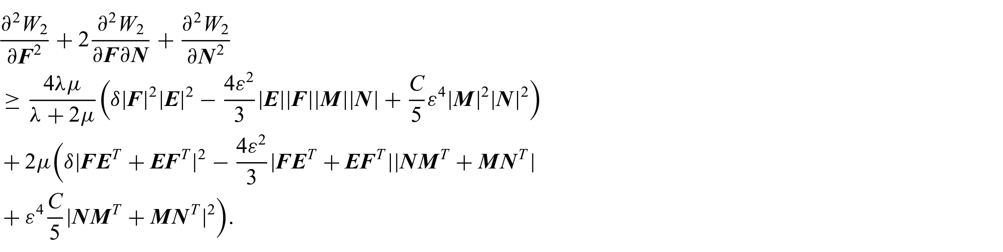
Combining the above three inequalities, we deduce that:
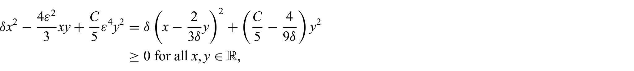
Then, inequality (20) is deduced by noting that the right-hand side of the above inequality is a non-negative scalar. Indeed,
if and only if and satisfy , which is precisely the assumption of the theorem on these constants. This completes the proof. □
Lemma 5.Let denote the diagonal matrix with and on its diagonal. Given any constants , , and and any positive function , let:
for all .
Assume that . Then:
whenever in when .
Proof. Given any matrix fields , define and a.e. . Then:
Let in when . Then:
Since the function is convex (the assumption that is used here), we have:
The conclusion follows by replacing by is this inequality.
5. A well-posed approximation of Koiter’s nonlinear shell model for planar shells
In this section, the middle surface of the shell satisfies:
where and , respectively, denote the mean and total curvatures along the surface (see section 2). This means that is a portion of a plane, so the immersion can be defined without losing in generality by:
Consequently,
where denotes the Kronecker symbol.
The purpose of this section is to define a nonlinear shell model that is well-posed and approaches the three-dimensional model of elasticity modeled by equation (11) with the same accuracy as Koiter’s nonlinear shell model. To this end, we will show that the coercive functional (16) can be approached by a new functional that is simultaneously coercive, sequentially weakly lower semi-continuous, and it approaches the three-dimensional energy functional (11) as well as Koiter’s functional (4).
To begin with, we define a new stored energy function, destined to replace the one appearing in the functional (16).
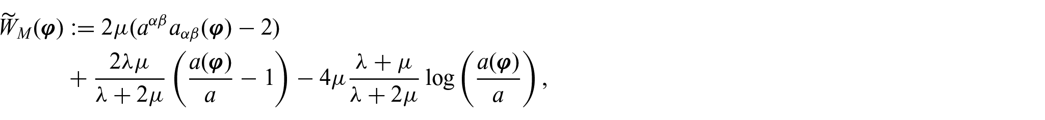
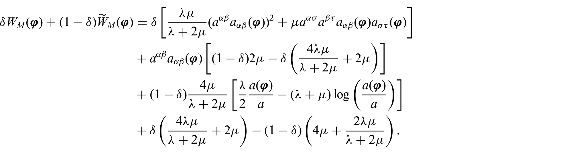
Definition 1. (stored energy function for planar shells). Let , , and be the functions defined in section 1, and let be the function defined in Lemma 2. Then, given any constants and , define the function by:
for all immersions such that .
The next theorem shows that coincides at the first order with Koiter’s stored energy function, viz.,
in terms of the change of metric and change of curvature tensor fields. Consequently, and approach the stored energy function of three-dimensional nonlinear elasticity with the same accuracy.
Theorem 1.For all immersions with that is sufficiently close in the -norm to the immersion , the following estimate hold:
Proof. First, Lemma 2 implies that:
Second, the assumption that the immersion is given by equation (21) implies that in , so that by Lemma 1 we have:
Using this estimate in the definition of then yields the estimate:
The conclusion follows using the above estimates for and in the definition of . □
The next theorem shows that the nonlinear shell model associated with the stored energy function defined in Definition 1 is well-posed as a minimization problem. Note that the theorem holds with the particular choices and irrespectively of the values of the elastic coefficients and .
Theorem 2. (existence of minimizers). Define the functional by:
where be the set defined by equation (18), be the function defined in Definition 1, and is any linear and continuous function.
Assume that that the constants and appearing in the definition of satisfy:
and that the set appearing in the definition of is non-empty. Then, has a minimizer in the set .
Proof. The proof is divided into five parts, denoted (1) to (5), for clarity.
(1) We first prove that is coercive.
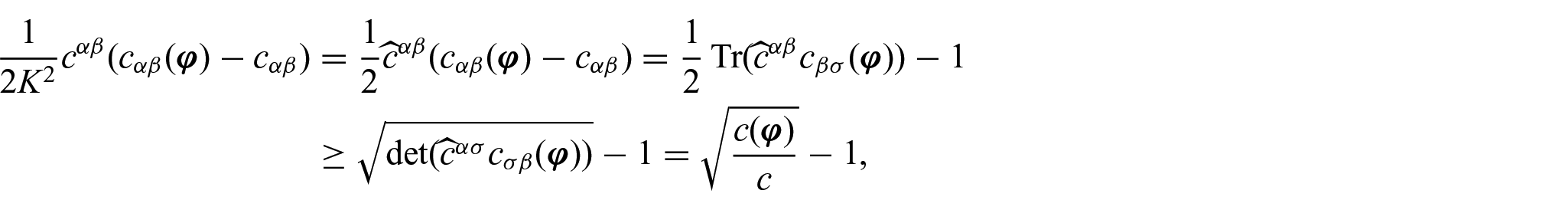
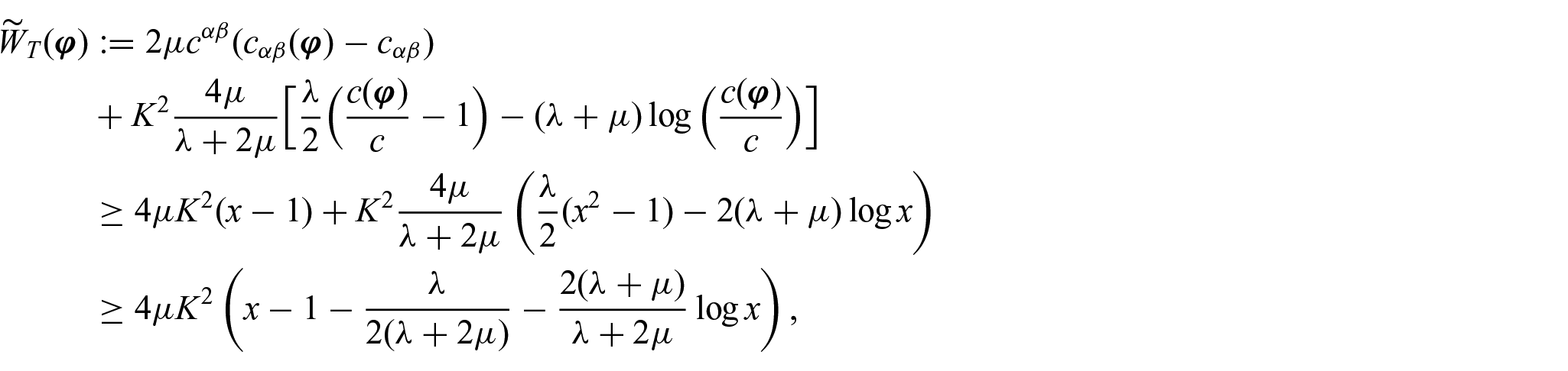
Let . Using the following generalized mean inequality:
in the definition of the function (cf. Lemma 2) shows that:
where . Then, an elementary computation of the infimum of the function in the right-hand side shows that:
where is a constant depending only on and . Note that the above inequality holds in particular for , but this particular value is not used in what follows.
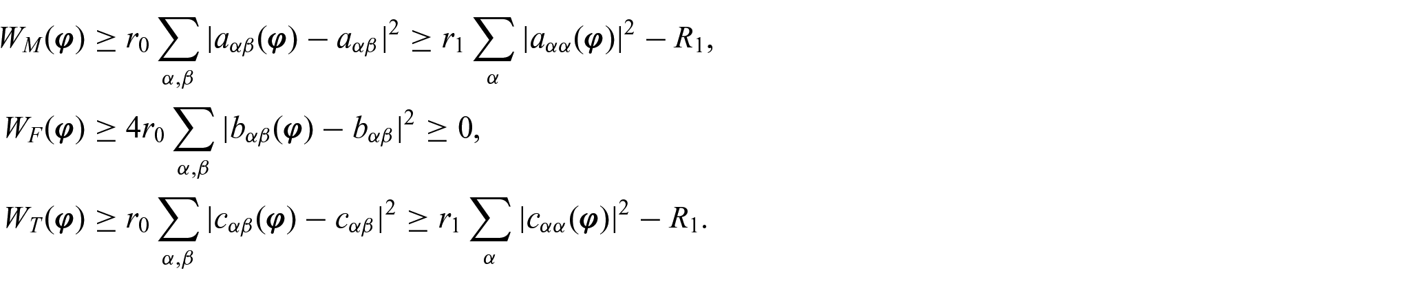
Besides, the uniform positive-definiteness of the two-dimensional elasticity tensor (1) (which is proven, for instance, in Ciarlet [2]) implies that there exist positive constants , , and such that, for all ,
and
Combining the above inequalities with Poincaré’s inequality in (which is bounded Lipschitz domain by assumption; cf. section 2) and using that and both belong to , one deduces that is well-defined as an extended real number in for all , that the functional defined in this fashion is bounded below, and that is coercive in the following sense: if a sequence satisfies:
then the sequences and , , are both bounded in .
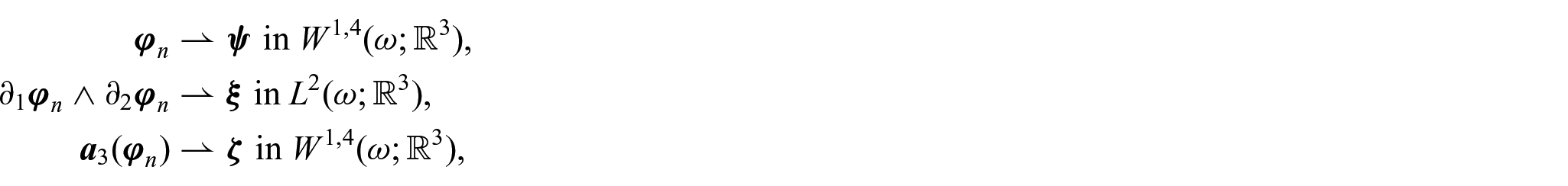
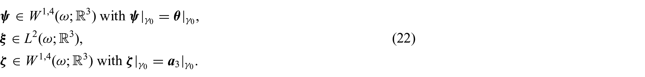
(2) Let denote an infimizing sequence of the functional over the set . Since contains at least one element, namely , we have . Then, the coerciveness of implies that the sequences and , , are both bounded in . This space being reflexive, there exists a subsequence, still denoted for conciseness, such that:
where:
Moreover, since:
we have:
(3) Next, we decompose into a sum of three particular functions, as follows. Since:
we have:
Note that the coefficient of is non-negative thanks to the assumption that .
Consequently,
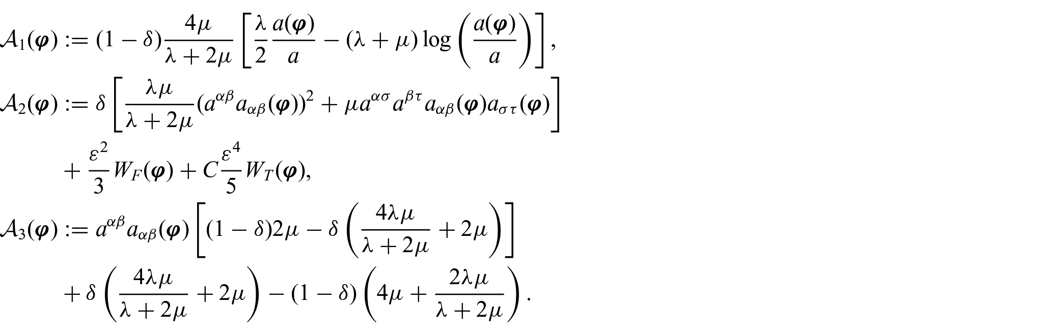
where:
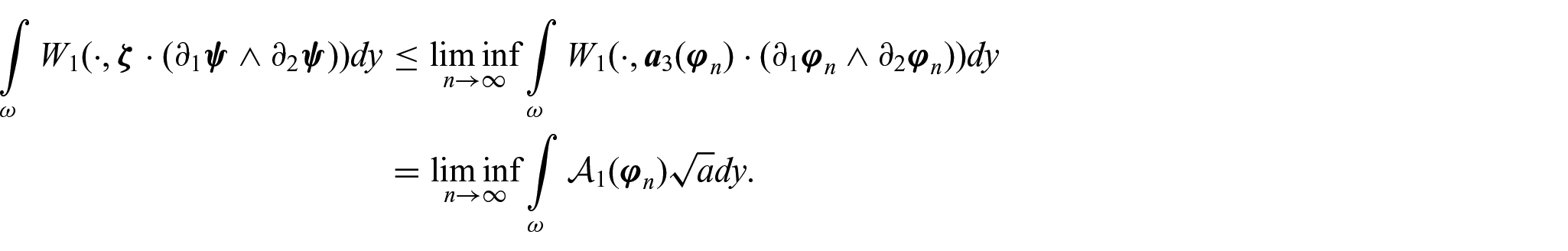
(4) We now prove that the integral of each function , , is sequentially weakly lower semi-continuous.
First, since:
the function can be recast in terms of the function defined in Lemma 3 with and as:
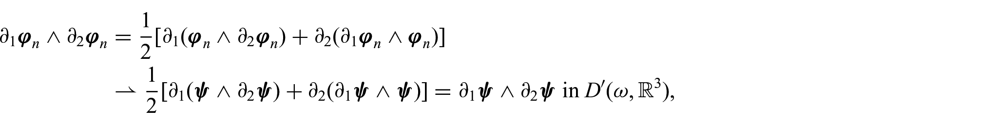
for all . The convergences established in (2) above and Sobolev’s embedding theorem showing that is compactly embedded in (see, for example, Adams [11] and remember that is a bounded Lipschitz domain in ), together imply that the sequence converges weakly in to the function . Then, Lemma 3 shows that:
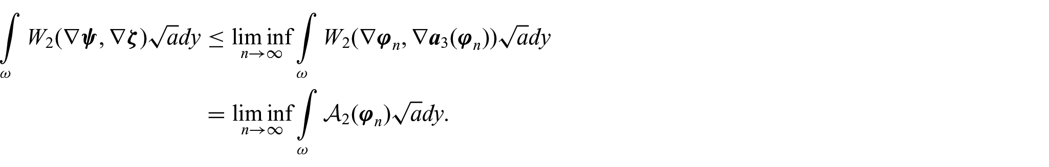
Second, using that and in , we deduce that:
for all immersions such that . Besides, denoting and , we also have:
Then, the above expression of can be recast as:
where the function is that defined in Lemma 4. Then, we infer from Lemma 4 that:
Third, using again that in , we have:
Since (we use here the upper bound of given in the statement of the theorem):
we infer from the definition of that:
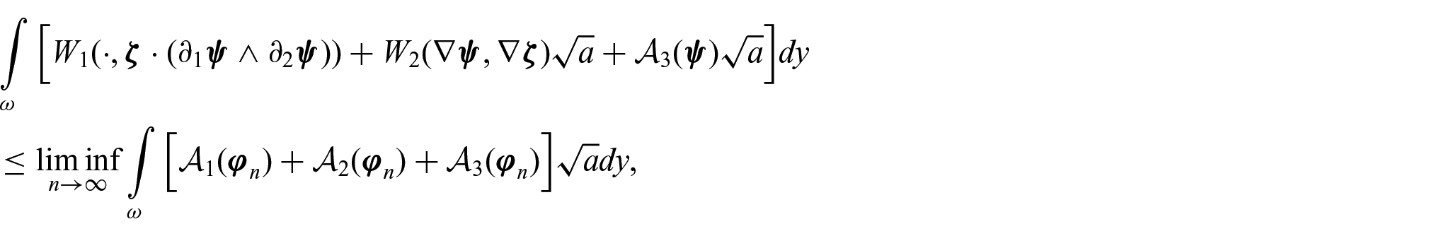
(5) The three inequalities established in part (4) of the proof together imply that:
then that, in view of relation (23),
Since , we deduce in particular that:
so that, by Lemma 3,
Furthermore, since and a.e. in , the convergences established in part (2) of the proof imply that:
The above relations show that is a positively oriented unit normal vector field to the surface , so that, in view of the comments preceding relations (8), we have:
Consequently, in view of the definition of the functions , , , and , we have:
and
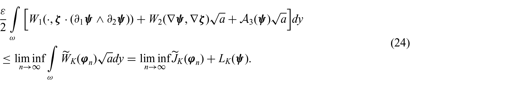
Then, inequality (24) can be recast as:
or equivalently, as:
Since relations (22) and (26) together imply that:
we have proved that the function minimizes the functional over .
The proof is complete.
6. A well-posed approximation of Koiter’s nonlinear shell model for non-planar minimal surfaces
The objective of this section is to establish an existence theorem, similar to the one in the previous section, to non-planar shells whose middle surface is a minimal surface: thus, throughout this section, the immersion defining the middle surface of the shell satisfies:
where and , respectively, denote the mean and total curvatures along the surface (see section 2). This assumption implies that the principal curvatures and of the surface (see section 2) satisfy:
for some positive function for all . Consequently, the total curvature of the surface satisfies:
By applying Cayley–Hamilton formula to the matrix field , one deduces that:
where denotes Kronecker’s symbol. Since in (see above) and in (see section 2), the above relation is equivalent to:
One then deduces that the covariant, resp. contravariant, components of the third fundamental form of satisfy (the operations of raising and lowering indices of tensor fields have been defined in section 2):
resp. (remember that denotes the inverse of the matrix field ; cf. section 2):
Since the matrix is symmetric and positive definite at every , so is the matrix ; hence, the inverse matrix:
is well-defined at each and it satisfies:
Note that the functions and are different functions, related to each other by the relation:
In what follows, we define a sequentially weakly lower semi-continuous approximation of Koiter’s energy for this type of shells (Definition 2), then we prove that the nonlinear shell model associated with this new energy is well-posed by proving that it possesses a global minimizer in the set of admissible deformations for Koiter’s model (Theorem 4).
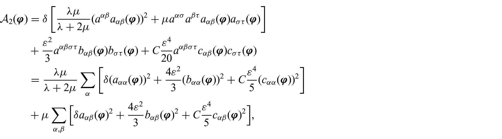
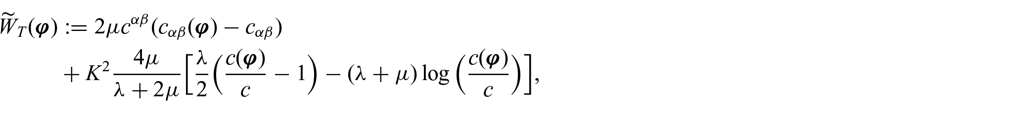
Definition 2. (stored energy function for non-planar shells). Let , , and be the functions defined in section 1, let be the function defined in Lemma 2, and, for each immersion such that , let be the function defined by:
at the points of where , and by at the other points.
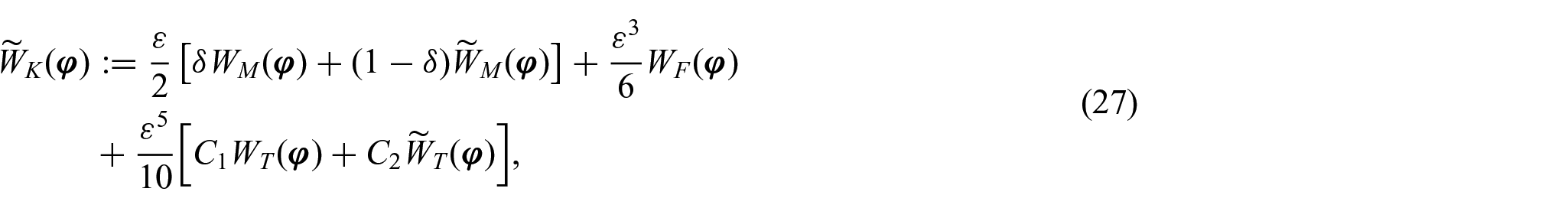
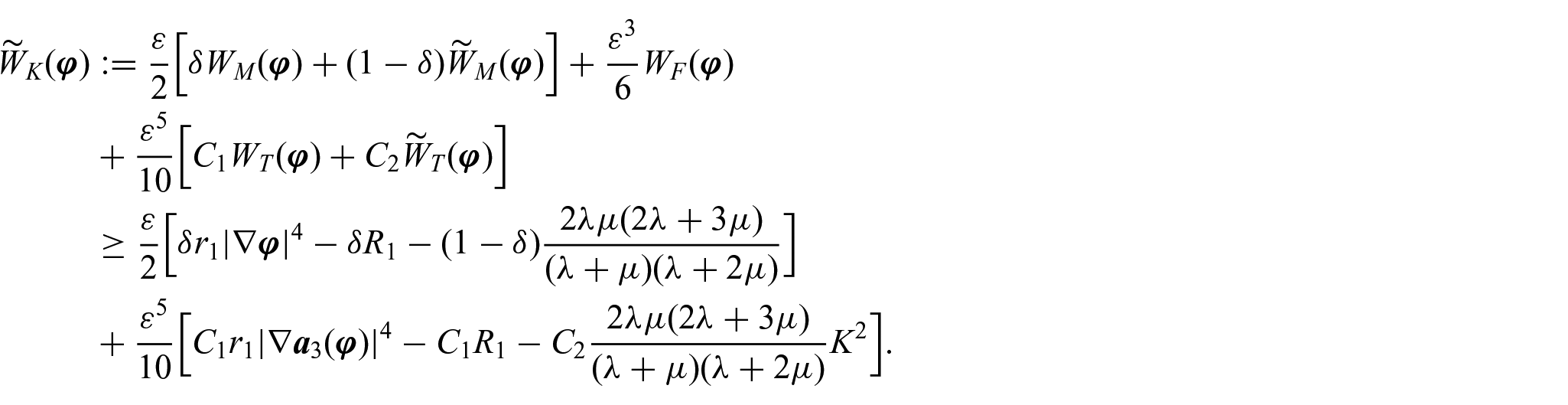
Then, given any constants , , , and , define the function by:
for each immersion such that .
The next theorem shows that the function defined by equation (27) coincides with Koiter’s stored energy function:
at the first order in terms of the change of metric and change of curvature tensor fields when the thickness is small enough. Consequently, approaches the stored energy function of three-dimensional nonlinear elasticity with the same accuracy as Koiter’s stored energy function .
Theorem 3.For any immersion that is sufficiently close in the -norm to the immersion with a unit normal field that is sufficiently close in the -norm to , the following estimate holds:
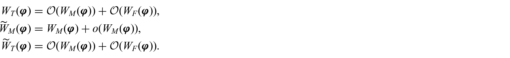
Proof. This estimate is a consequence of the following three estimates:
The first two estimates were established, respectively, in Lemmas 1 and 2. The last estimate is established below.
The definition of the functions (see section 2) implies that:
Consequently,
on one hand.
On the other hand, Cayley–Hamilton theorem applied to the matrix field , where , shows that:
where denotes Kronecker’s symbol, which next implies that (by applying the trace operator to the above matrix equation):
Using this formula in the previous expression of the function shows that:
which in turn implies that:
Using the above estimates in the definition of the function (see Definition 2) next shows that:
Then, the desired estimate for the function is obtained using the relations and (which are proved at the beginning of this section) in this formula.
The next theorem shows that the nonlinear shell model associated with the stored energy function is well-posed. Note that the theorem holds with the particular choices , , and irrespectively of the values of the elastic coefficients and .
Theorem 4. (existence of minimizers). Define the functional by:
where is the set defined by equation (18), is the function defined by equation (27), and is any linear and continuous function.
Assume that the constants appearing in the definition of satisfy , , and
Then, the functional has a minimizer in .
Proof. The proof is divided into four parts, denoted (1) to (4), for clarity.
(1) We have shown in step (1) of the proof of Theorem 2 that, a.e. in ,
for all . The proof did not use the particular assumption made in section 5 on the immersion , so the above estimate holds for any given immersion in , hence in particular under the assumption on made in this section.
Next, using the following generalized mean inequality:
we deduce that, a.e. in ,
which in turn implies that, again a.e. in ,
where . Then, the same elementary computation of the infimum of the function in the right-hand side as the one in part (1) of the proof of Theorem 2 shows that, a.e. in ,
Finally, it is clear the uniform positive-definiteness of the two-dimensional elasticity tensor defined by equation (1) that there exist positive constants , and , all of them depending only on , and , such that, a.e. in ,
Using the above inequalities in Definition (27) of , shows that, a.e. in ,
This inequality and Poincaré’s inequality in (remember that is a bounded Lipschitz domain by assumption; cf. section 2) together show that the functional is well-defined as an extended real number in for all , and that there exist two constants and such that:
for all . Since in addition for all , the infimum of the functional over the set is a real number.
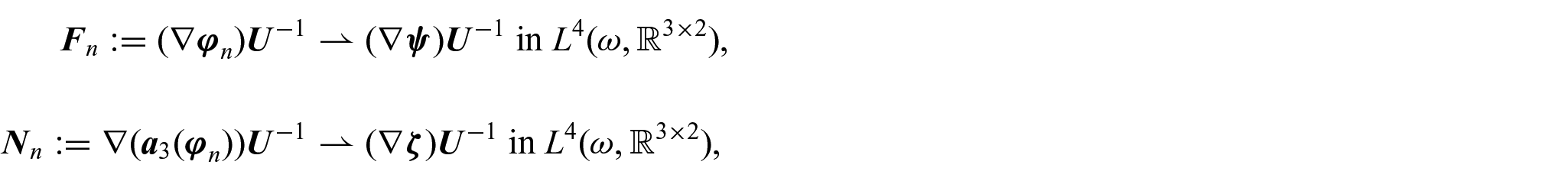
Let denote an infimizing sequence of the functional over the set . Then, the above inequalities and Poincaré’s inequality in (remember that is a bounded Lipschitz domain by assumption) together imply that both sequences and , , are bounded in . This space being reflexive, there exists a subsequence, still denoted for conciseness and functions:
such that:
Then, a compactness by compensation argument (the same as the one used in step (1) of the proof of Theorem 2) shows that:
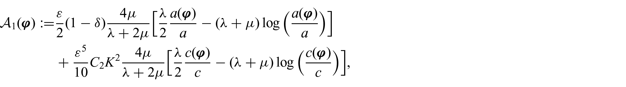
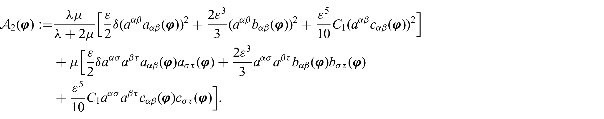
(2) Let be any element in . The assumption that the mean curvature satisfies in allows to decompose the function into the following sum:
where the functions in the right-hand side are defined as follows.
The function is defined by:
at the points of where , and by at the points of where .
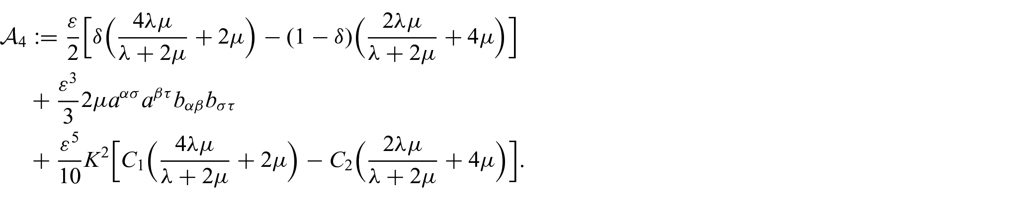
The function is defined by:
The function is defined by:
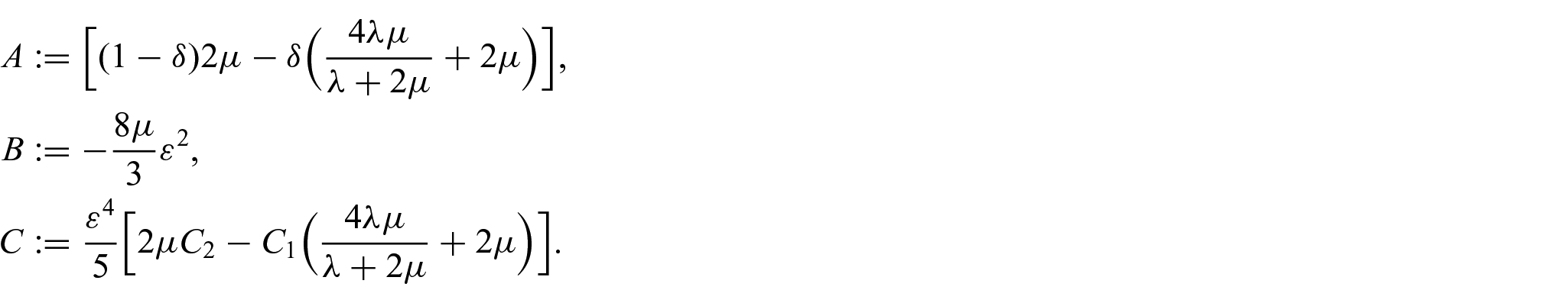
where:
Finally, the function is a function independent of defined by:
(3) We now prove that the integral of each function , , is sequentially weakly lower semi-continuous. First, since:
and
the function satisfies:
where , resp. , denotes the function defined in Lemma 3 with and , resp. with and . Since the sequences and both converge weakly in , respectively, to the functions and thanks to the convergences established in (1) above combined with the compact embedding of into (remember that is a bounded Lipschitz domain in ), Lemma 3 implies that:
Second, since the matrix is symmetric and positive definite at each , there exists a unique symmetric and positive definite matrix such that:
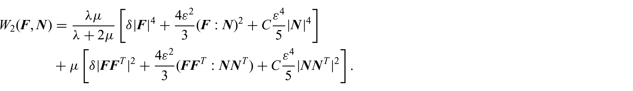
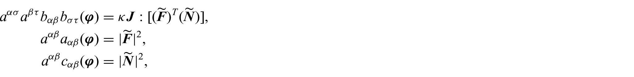
Let and . Then, a series of straightforward calculations show that, for all immersion such that , the following relations hold a.e. in :
where the notation : denotes the inner product between two matrices of the same type.
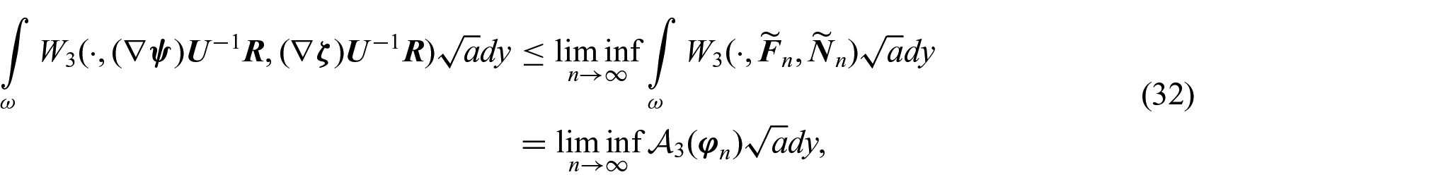
Using these relations in the definition of implies that:
where the function is that defined in the statement of Lemma 4 with constant replaced by the constant appearing in the definition of the function . Therefore, since the convergences (29) imply that:
we infer from Lemma 4 that:
Third, since the matrix field satisfies in , the assumption that the mean curvature of the surface satisfies in implies that:
and the assumption that the total curvature of satisfies in implies that:
The matrix field being symmetric, the two previous relations together imply that there exists a field of orthogonal matrices such that:
where denotes the diagonal matrix with and on its diagonal. Then, a series of straightforward calculations show that the following relations hold a.e. in :
where and. Then, we infer from the definition of the function that:
where is the function defined in Lemma 5.
That the constants , and satisfy the assumptions of the theorem amount to the condition that the coefficients of the function satisfy:
which means that the function satisfies all the assumptions of Lemma 5. Therefore:
since the convergences (29) imply that, when ,
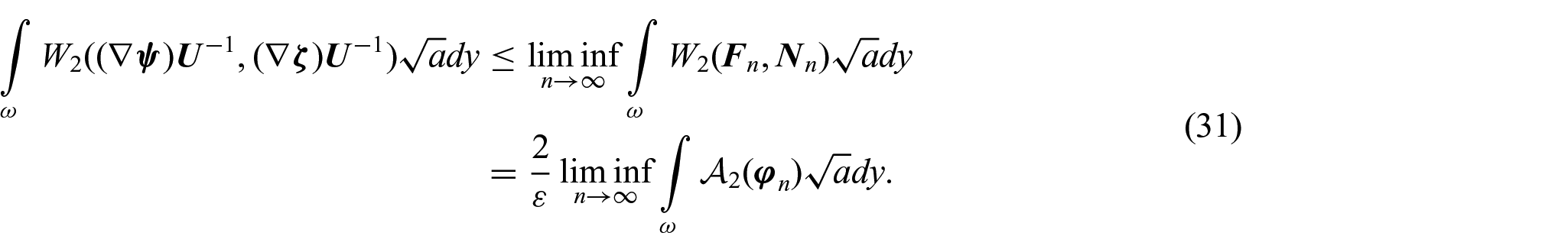
(4) Adding the three inequalities (30), (31), and (32) established above shows that:
Then, since , we deduce in particular that:
so that, by Lemma 3,
Besides, since and a.e. in , the convergences established in part (1) of the proof imply that:
The last two relations together show that is a unit normal vector field to the surface that is positively oriented, so that, in view of the observation preceding relations (8) in section 2, we have:
Consequently, in view of the definition of the functions and in terms of the functions , , and , we have:
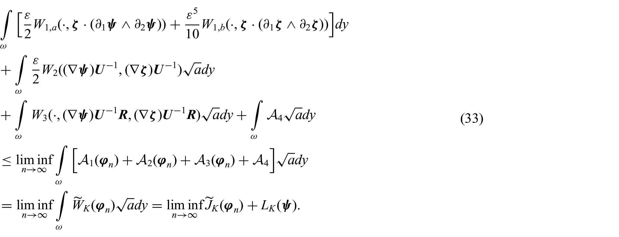
Then, inequality (33) can be recast as:
or equivalently, as:
Since relations (28) and (34) together imply that:
we have proved that the function minimizes the functional over .
The proof is complete.
Footnotes
Funding
The author(s) disclosed receipt of the following financial support for the research, authorship, and/or publication of this article: The work described in this paper was substantially supported by a grant from City University of Hong Kong (Project no. 7005608).
ORCID iDs
Trung Hieu Giang
Cristinel Mardare
References
1.
KoiterWT.On the nonlinear theory of thin elastic shells. Proc Kon Ned Akad Wetensch1966; B69: 1–54.
2.
CiarletPG.Mathematical elasticity, vol. III: theory of shells. Amsterdam: North-Holland, 2000.
3.
BallJMCurrieJCOlverPJ.Null Lagrangians, weak continuity, and variational problems of arbitrary order. J Funct Anal1981; 41(2): 135–174.
4.
CiarletPGGoguRMardareC.Orientation-preserving condition and polyconvexity on a surface: application to nonlinear shell theory. J Math Pures Appl2013; 99: 704–725.
5.
BunoiuBCiarletPGMardareC.Existence theorem for a nonlinear elliptic shell model. J Elliptic Parabolic Eqns2015; 1: 31–48.
6.
CiarletPGMardareC.A mathematical model of Koiter’s type for a nonlinearly elastic “almost spherical” shell. CR Acad Sci Paris Ser I2016; 354: 1241–1247.
7.
AnicicS.Existence theorem for a first-order Koiter nonlinear shell model. Discrete Contin Dyn Syst - S2019; 12: 1535–1545.
8.
AnicicS.Polyconvexity and existence theorem for nonlinearly elastic shells. J Elast2018; 132: 161–173.
9.
CiarletPGMardareC.An existence theorem for a two-dimensional nonlinear shell model of Koiter’s type. Math Models Meth Appl Sci2018; 28: 2833–2861.
10.
MardareC.Nonlinear shell models of Kirchhoff-Love type: existence theorem and comparison with Koiter’s model. Acta Math Appl Sin Engl Ser2019; 35: 3–27.