Tensor decomposition for modified quasi-linear viscoelastic models: Towards a fully non-linear theory

Abstract

We discuss the decomposition of the tensorial relaxation function for isotropic and transversely isotropic (TI) modified quasi-linear viscoelastic (MQLV) models. We show how to formulate the constitutive equation using a convenient decomposition of the relaxation tensor into scalar components and tensorial bases. We show that the bases must be symmetrically additive, i.e., they must sum up to the symmetric fourth-order identity tensor. This is a fundamental property both for isotropic and anisotropic bases that ensures the constitutive equation is consistent with the elastic limit. We provide two robust methods to obtain such bases. Furthermore, we show that, in the TI case, the bases are naturally deformation-dependent for deformation modes that induce rotation or stretching of the fibres. Therefore, the MQLV framework allows to capture the non-linear phenomenon of strain-dependent relaxation, which has always been a criticised limitation of the original quasi-linear viscoelastic theory. We illustrate this intrinsic non-linear feature, unique to the MQLV model, with two examples (uni-axial extension and perpendicular shear).

1. Introduction: linear, quasi-linear, and modified quasi-linear viscoelasticity

According to the classical linear theory, the constitutive equation for a viscoelastic material in the integral form can be written down under the following assumptions: the material remembers the past deformation history through a fading memory, so that contributions to recent strain increments are more important than past contributions, the total stress at the current time $t$ is given by the sum of all past stress contributions (the Boltzmann superposition principle), and the material is subjected to small deformations [1]. Moreover, by taking the deformation history to start at $t=0$ , the stress can be written as follows:

$$\mathbf{\sigma }(t)={\int }_0^t\mathbb{G}(t-\tau ):\frac{\mathrm{d}{\mathbf{\sigma }}^{\mathrm{e}}(\tau )}{\mathrm{d}\tau }\mathrm{d}\tau ,$$

(1)

where ${\mathbf{\sigma }}^{\mathrm{e}}$ is the elastic stress tensor, and $\mathbb{G}$ is the reduced relaxation tensor. $\mathbb{G}$ is the fourth-order tensor whose components are the time-dependent material functions that dictate the relaxation behaviour of the material. As is the case for any fourth-order tensor, $\mathbb{G}$ can be decomposed into its components:

$$\mathbb{G}(t)=\sum _{n=1}^N{G}_n(t){\mathbb{K}}_n(t),$$

(2)

upon choosing a set of fourth-order bases ${\mathbb{K}}_n$ , for $n=1,\dots ,N$ ( $N$ being the total number of independent components). The components of the reduced relaxation function satisfy the condition $G_n(0)=1$ for $n=1,\dots ,N$ . The functional form of the components of $\mathbb{G}$ is generally chosen with the help of experiments. A stress relaxation test can be performed where the material is suddenly deformed and then held in position for a certain time. The shape of the resulting stress curve over time will dictate the form of the relaxation function, for instance, soft tissues typically display an exponentially decaying relaxation behaviour [2, 3].

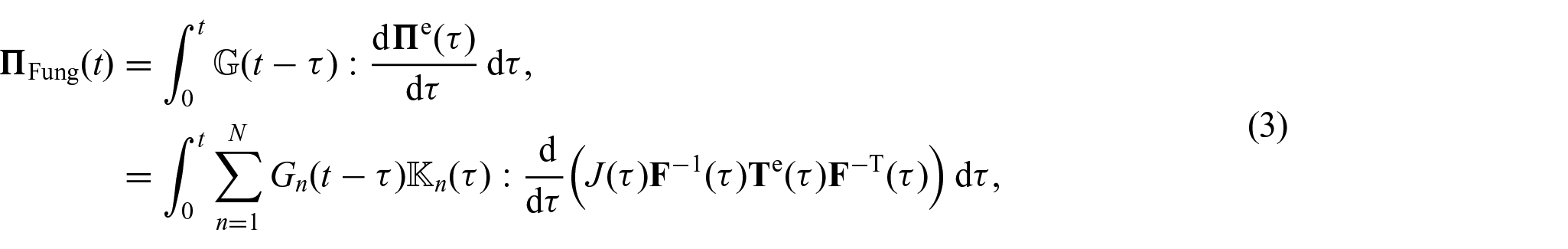
Equation (1) is valid in the small deformation regime; therefore, it has little application in soft tissue mechanics, where the tissues may be stretched up to twice their initial length [4, 5]. To overcome this limitation, Fung proposed what is now called the quasi-linear viscoelastic (QLV) constitutive framework [6]. The basis of Fung’s idea is to extend equation (1) to finite deformations. In the large deformation setting, the deformation of a continuum body is modelled as a linear function $\mathit{\chi }$ (in three-dimensional (3D) Euclidean space) that transforms points from an initial undeformed state to a final deformed state. We use the notation $\mathbf{X}$ and $\mathbf{x}(t)$ to denote position vectors in the undeformed and deformed states, respectively, so that $\mathbf{x}(t)=\mathit{\chi }(t,\mathbf{X})$ . The gradient of the deformation is the tensor $\mathbf{F}(t)=\frac{\partial \mathbf{x}(t)}{\partial \mathbf{X}}$ . Mathematically, the constitutive equation in the QLV framework is written with respect to the second Piola–Kirchhoff stress tensor in the following form:

$$\begin{array}{c}{\mathbf{\Pi }}_{\mathrm{Fung}}(t)={\int }_0^t\mathbb{G}(t-\tau ):\frac{\mathrm{d}{\mathbf{\Pi }}^{\mathrm{e}}(\tau )}{\mathrm{d}\tau }\mathrm{d}\tau ,\hfill \\ \multicolumn{1}{c}{={\int }_0^t\sum _{n=1}^N{G}_n(t-\tau ){\mathbb{K}}_n(\tau ):\frac{\mathrm{d}}{\mathrm{d}\tau }(J(\tau ){\mathbf{F}}^{-1}(\tau ){\mathbf{T}}^{\mathrm{e}}(\tau ){\mathbf{F}}^{-\mathrm{T}}(\tau ))\mathrm{d}\tau ,}\end{array}$$

(3)

where $J$ is the determinant of the deformation gradient $\mathbf{F}$ , ${\mathbf{\Pi }}^{\mathrm{e}}$ is the elastic second Piola–Kirchhoff stress tensor, and ${\mathbf{T}}^{\mathrm{e}}$ is the elastic Cauchy stress tensor. The second Piola–Kirchhoff and the Cauchy stress tensors are linked via the Piola transformation $\mathbf{\Pi }=J{\mathbf{F}}^{-1}\mathbf{T}{\mathbf{F}}^{-\mathrm{T}}$ . The QLV framework has three main advantages: (1) the constitutive equation (3) can account for the non-linear elastic behaviour of a material, through the tensor ${\mathbf{\Pi }}^{\mathrm{e}}$ ; (2) the tensor $\mathbb{G}$ can be fully determined from experiments performed in the small deformation regime, and this follows from the fact that the reduced relaxation tensor is inherited by the QLV model directly from the linear theory (see equation (1)); and (3) when it comes to modelling experimental data, a constitutive equation should be written with respect to physically measurable parameters that can be determined straightforwardly via experiment. In principle, this can be achieved for equation (3) upon choosing an appropriate set of bases to split the reduced relaxation tensor $\mathbb{G}$ into components that are associated with specific deformation modes.

With this aim, the QLV theory has recently been revisited for isotropic and transversely isotropic materials (TI) in De Pascalis et al. [7] and Balbi et al. [8], respectively. In these two works, the authors proposed a modified version of the quasi-linear viscoelastic theory (MQLV) where the split acts on the Cauchy stress tensor directly:

$$\begin{array}{c}\mathbf{\Pi }(t)=J(t){\mathbf{F}}^{-1}(t)(\mathbb{G}(0):{\mathbf{T}}^{\mathrm{e}}(t)){\mathbf{F}}^{-\mathrm{T}}(t)\hfill \\ \multicolumn{1}{c}{+{\int }_0^{t}J(\tau ){\mathbf{F}}^{-1}(\tau )({\mathbb{G}}^{\prime }(t-\tau ):{\mathbf{T}}^{\mathrm{e}}(\tau )){\mathbf{F}}^{-\mathrm{T}}(\tau )\mathrm{d}\tau .}\end{array}$$

(4)

here, ’ indicates the differentiation with respect to the argument. This choice is motivated by the fact that the Cauchy stress has a physical meaning, representing the actual stress distribution in the material, as opposed to the second Piola–Kirchhoff stress. The problem now amounts to finding a set of bases ${\mathbb{K}}_n(t)$ such that the associated components $G_n(t)$ also have a physical meaning and can then be experimentally measured by common testing protocols (tensile, compression, bi-axial, shear, or torsion tests). The question of splitting isotropic and anisotropic tensors has been investigated in previous works in the context of elasticity [9, 10]. However, as we show in this paper, these results are not applicable to the QLV framework because the splits discussed in the literature [9, 10] would yield a constitutive equation that does not recover the elastic limit.

In this paper, we show for the first time that the tensorial bases must be symmetrically additive, i.e., they must sum up to the fourth-order symmetric identity tensor $\mathbb{S}$ . Additive symmetry is a fundamental property that ensures the constitutive equation recovers the elastic limit. For the first time, we propose two different methods to derive symmetrically additive set of bases for isotropic and TI tensors, respectively. Finally, we show that for anisotropic materials, the tensorial bases depend on the deformation through a vector that defines the axis of anisotropy. This feature allows us to capture the non-linear phenomenon of strain-dependent relaxation for TI materials and opens the way to develop fully non-linear viscoelastic models within the QLV framework. Non-linear phenomena are displayed by soft matter such as polymers, hydrogels, and biomaterials, which are used to mimic soft tissue mechanics and in bio-robotics applications [11, 12]. Therefore, developing viscoelastic models that can capture non-linearities is crucial in order to improve the design of such materials.

For completeness, we recall that, alongside integral formulations, other approaches, such as differential type models (also called internal variables models), have been proposed in the literature to model viscoelasticity [13–15]. These models assume that the total energy can be decomposed into the sum of an elastic and a viscous part. The elastic part depends on the deformation only, whereas the viscous part depends both on the deformation and on some internal variables. Accordingly, the deformation gradient is split, via a multiplicative decomposition, into an elastic part and a viscous part. The evolution laws for the internal variables are usually dictated by thermodynamics principles. Differential type models are particularly convenient for numerical implementation in finite element codes. However, it is not always clear how the internal variables are linked to physically measurable parameters.

We organise this paper as follows. We first introduce the additive symmetry property, starting by considering the isotropic case. We then move on to the TI case. Finally, we apply the results of the previous sections to the MQLV theory. We show that the MQLV framework naturally incorporates strain-dependent relaxation, a non-linear feature that has always been a strong limitation of the original QLV theory.

2. Fourth-order bases for isotropic materials

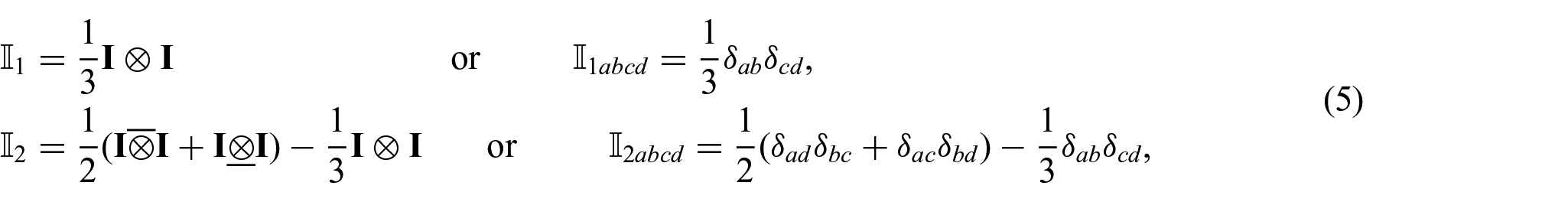
We start by considering the isotropic case. From the theory of elasticity, we know that the elasticity tensor for an isotropic material has two independent components. The material properties of a linearly elastic material are uniquely identified by any of the following pairs of parameters: the first Lamé constant $\lambda$ and the shear modulus $\mu$ , the bulk modulus $\kappa$ and $\mu$ , and Young’s modulus $E$ and Poisson’s ratio $\nu$ . Each pair is associated with a different set of bases. For instance, the set of bases:

$$\begin{array}{c}{\mathbb{I}}_1=\frac{1}{3}\mathbf{I}\otimes \mathbf{I}\mathrm{or}{\mathbb{I}}_{1\mathrm{abcd}}=\frac{1}{3}{\delta }_{\mathrm{ab}}{\delta }_{\mathrm{cd}},\hfill \\ \multicolumn{1}{c}{{\mathbb{I}}_2=\frac{1}{2}(\mathbf{I}\overline{\otimes }\mathbf{I}+\mathbf{I}\underset{¯}{\otimes }\mathbf{I})-\frac{1}{3}\mathbf{I}\otimes \mathbf{I}\mathrm{or}{\mathbb{I}}_{2\mathrm{abcd}}=\frac{1}{2}({\delta }_{\mathrm{ad}}{\delta }_{\mathrm{bc}}+{\delta }_{\mathrm{ac}}{\delta }_{\mathrm{bd}})-\frac{1}{3}{\delta }_{\mathrm{ab}}{\delta }_{\mathrm{cd}},}\end{array}$$

(5)

yields the following constitutive equation for a linearly elastic isotropic material:

$${\mathbf{\sigma }}^e=\mathbb{C}:\mathit{\epsilon }=\sum _{n=1}^2{C}_n{\mathbb{I}}_n:\mathit{\epsilon }=\kappa \mathrm{tr}[\mathit{\epsilon }]\mathbf{I}+2\mu \mathrm{dev}[\mathit{\epsilon }],$$

(6)

where $C_1=3\kappa$ and $C_2=2\mu$ and $\mathrm{dev}[\mathit{\epsilon }]=\mathit{\epsilon }-\frac{1}{3}\mathrm{tr}[\mathit{\epsilon }]\mathbf{I}$ .

The bases $\{{\mathbb{I}}_1,{\mathbb{I}}_2\}$ have the following important properties: idempotence, orthogonality, and additive symmetry.

Property 1 Idempotence under double contraction:

$${\mathbb{I}}_1:{\mathbb{I}}_1={\mathbb{I}}_1,{\mathbb{I}}_2:{\mathbb{I}}_2={\mathbb{I}}_2.$$

(7)

Property 2 Orthogonality:

$${\mathbb{I}}_1:{\mathbb{I}}_2=\mathbb{O},{\mathbb{I}}_2:{\mathbb{I}}_1=\mathbb{O},$$

(8)

where $\mathbb{O}$ is the fourth-order null tensor, with components ${\mathbb{O}}_{\mathrm{abcd}}=0$ , $\forall a,b,c,d$ .

Property 3 Additive symmetry:

$${\mathbb{I}}_1+{\mathbb{I}}_2=\mathbb{S},$$

(9)

where $\mathbb{S}$ is the symmetric fourth-order identity tensor in equation (75).

Please see Appendix 1 for proofs of these properties.

For symmetric tensors $\mathbf{U}={\mathbf{U}}^{\mathrm{T}}$ , as shown in equation (79) (see Appendix 1), the tensor $\mathbb{S}$ acts as the fourth-order identity tensor $\underset{¯}{\mathbb{I}}$ . Therefore:

$$\underset{¯}{\mathbb{I}}:\mathbf{U}=\mathbb{S}:\mathbf{U}=({\mathbb{I}}_1+{\mathbb{I}}_2):\mathbf{U}=\frac{1}{3}\mathrm{tr}[\mathbf{U}]\mathbf{I}+(\mathbf{U}-\frac{1}{3}\mathrm{tr}[\mathbf{U}]\mathbf{I})=\mathbf{U}.$$

(10)

Equation (10) shows that the set of symmetrically additive bases $\{{\mathbb{I}}_1,{\mathbb{I}}_2\}$ can be used to split a symmetric second-order tensor into the sum of two terms. Although this is a well-known result, it plays a crucial role in the viscoelastic setting, as we show later in this paper.

Let us now consider the set of bases:

$${\hat{\mathbb{I}}}_1=\mathbf{I}\otimes \mathbf{I}=3{\mathbb{I}}_1\mathrm{and}{\hat{\mathbb{I}}}_2=\frac{1}{2}(\mathbf{I}\overline{\otimes }\mathbf{I}+\mathbf{I}\underset{¯}{\otimes }\mathbf{I})={\mathbb{I}}_1+{\mathbb{I}}_2.$$

(11)

They are linked to the bases in equation (5) by the following connections: ${\hat{\mathbb{I}}}_1=3{\mathbb{I}}_1$ and ${\hat{\mathbb{I}}}_2={\mathbb{I}}_2+{\mathbb{I}}_1$ . The set of bases in equation (11) allows us to write the constitutive equation for a linear elastic material as follows:

$${\mathbf{\sigma }}^{\mathrm{e}}=\mathbb{C}:\mathit{\epsilon }=\sum _{n=1}^N{\hat{C}}_n{\hat{\mathbb{I}}}_n:\mathit{\epsilon }=\lambda \mathrm{tr}[\mathit{\epsilon }]\mathbf{I}+2\mu \mathit{\epsilon },$$

(12)

where ${\hat{C}}_1=\lambda$ and ${\hat{C}}_2=2\mu$ . By comparing equations (6) and (12) we obtain the following links between the components $C_n$ $(n=1,2)$ associated with the set of bases in equation (5) and the components ${\hat{C}}_n$ associated with the bases in equation (11), i.e.:

$${\hat{C}}_1=\frac{C_1-C_2}{3}\mathrm{and}{\hat{C}}_2=C_2.$$

(13)

From equation (13), we can recover the well-known relation between the first Lamé constant and the bulk modulus, $\lambda =\kappa -23\mu$ . We can easily verify that, although the two constitutive equations in equations (6) and (12) are equivalent, the bases in equations (5) and (11) do not share the same properties. Indeed, the set in equation (11) has none of the three properties. In particular, the bases $\{{\hat{\mathbb{I}}}_1,{\hat{\mathbb{I}}}_2\}$ do not have the additive symmetry property:

$$({\hat{\mathbb{I}}}_1+{\hat{\mathbb{I}}}_2):\mathbf{U}=\mathrm{tr}[\mathbf{U}]\mathbf{I}+\mathbf{U}\ne \mathbf{U}.$$

(14)

2.1. Linear viscoelasticity

Let us now consider the viscoelastic setting. In the same fashion as for the elastic setting, we want to find some set of bases for the tensor $\mathbb{G}$ that allows us to rewrite the constitutive equation in equation (1) with respect to different relaxation functions. In particular, we would like the relaxation functions to be associated with deformation modes that can be performed experimentally. The constitutive form (1) is written with respect to the elastic stress and the reduced relaxation tensor and is a convenient form to later make the link with the MQLV theory.

Integration by parts of equation (1) gives:

$$\sigma (t)=\underset{\mathrm{elastic}\mathrm{stress}}{\underbrace{\mathbb{G}(0):{\mathbf{\sigma }}^{\mathrm{e}}(t)}}+{\int }_0^t{\mathbb{G}}^{\prime }(t-\tau ):{\mathbf{\sigma }}^{\mathrm{e}}(\tau )\mathrm{d}\tau .$$

(15)

Since $\mathbb{G}$ is the reduced relaxation tensor, its components satisfy the condition $G_n(0)=1,\forall n$ . Now, let $\{{\mathbb{K}}_1,{\mathbb{K}}_2\}$ be the set of bases associated with the components $\{G_1,G_2\}$ , and then the term outside the integral must give the elastic stress ${\mathbf{\sigma }}^{\mathrm{e}}(t)$ :

$$\sum _{n=0}^2{G}_n(0){\mathbb{K}}_n:{\mathbf{\sigma }}^{\mathrm{e}}(t)=\sum _{n=0}^2{\mathbb{K}}_n:{\mathbf{\sigma }}^{\mathrm{e}}(t)\equiv {\mathbf{\sigma }}^{\mathrm{e}}(t).$$

(16)

Therefore, the bases ${\mathbb{K}}_n$ must possess the property of additive symmetry. This property is crucial in order for the constitutive equation to recover the elastic limit.

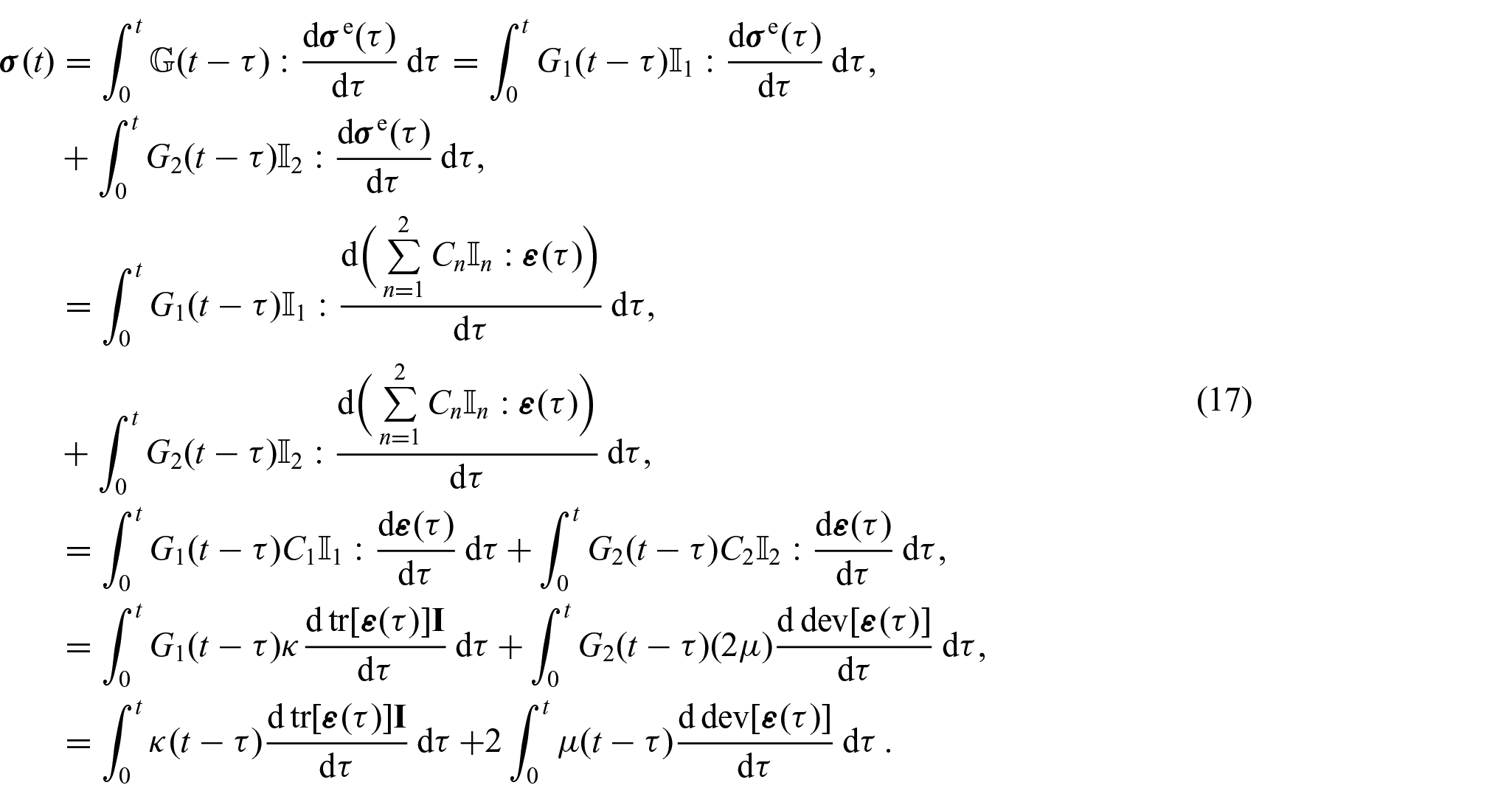
We can now show how to write the constitutive equation for a linear viscoelastic material in different forms, each with different relaxation functions. Since the bases $\{{\mathbb{I}}_1,{\mathbb{I}}_2\}$ in equation (5) are symmetrically additive, we can use them to split the tensor $\mathbb{G}$ , as follows:

$$\begin{array}{c}\mathbf{\sigma }(t)={\int }_0^t\mathbb{G}(t-\tau ):\frac{\mathrm{d}{\mathbf{\sigma }}^{\mathrm{e}}(\tau )}{\mathrm{d}\tau }\mathrm{d}\tau ={\int }_0^t{G}_1(t-\tau ){\mathbb{I}}_1:\frac{\mathrm{d}{\mathbf{\sigma }}^{\mathrm{e}}(\tau )}{\mathrm{d}\tau }\mathrm{d}\tau ,\hfill \\ \multicolumn{1}{c}{+{\int }_0^t{G}_2(t-\tau ){\mathbb{I}}_2:\frac{\mathrm{d}{\mathbf{\sigma }}^{\mathrm{e}}(\tau )}{\mathrm{d}\tau }\mathrm{d}\tau ,}\\ \multicolumn{1}{c}{={\int }_0^t{G}_1(t-\tau ){\mathbb{I}}_1:\frac{\mathrm{d}(\sum _{n=1}^2{C}_n{\mathbb{I}}_n:\mathit{\epsilon }(\tau ))}{\mathrm{d}\tau }\mathrm{d}\tau ,}\\ \multicolumn{1}{c}{+{\int }_0^t{G}_2(t-\tau ){\mathbb{I}}_2:\frac{\mathrm{d}(\sum _{n=1}^2{C}_n{\mathbb{I}}_n:\mathit{\epsilon }(\tau ))}{\mathrm{d}\tau }\mathrm{d}\tau ,}\\ \multicolumn{1}{c}{={\int }_0^t{G}_1(t-\tau )C_1{\mathbb{I}}_1:\frac{\mathrm{d}\mathit{\epsilon }(\tau )}{\mathrm{d}\tau }\mathrm{d}\tau +{\int }_0^t{G}_2(t-\tau )C_2{\mathbb{I}}_2:\frac{\mathrm{d}\mathit{\epsilon }(\tau )}{\mathrm{d}\tau }\mathrm{d}\tau ,}\\ \multicolumn{1}{c}{={\int }_0^t{G}_1(t-\tau )\kappa \frac{\mathrm{d}\mathrm{tr}[\mathit{\epsilon }(\tau )]\mathbf{I}}{\mathrm{d}\tau }\mathrm{d}\tau +{\int }_0^t{G}_2(t-\tau )(2\mu )\frac{\mathrm{d}\mathrm{dev}[\mathit{\epsilon }(\tau )]}{\mathrm{d}\tau }\mathrm{d}\tau ,}\\ \multicolumn{1}{c}{={\int }_0^t\kappa (t-\tau )\frac{\mathrm{d}\mathrm{tr}[\mathit{\epsilon }(\tau )]\mathbf{I}}{\mathrm{d}\tau }\mathrm{d}\tau +2{\int }_0^t\mu (t-\tau )\frac{\mathrm{d}\mathrm{dev}[\mathit{\epsilon }(\tau )]}{\mathrm{d}\tau }\mathrm{d}\tau .}\end{array}$$

(17)

In equation (17), we used equation (6) to write the elastic stress ${\mathbf{\sigma }}^{\mathrm{e}}$ in terms of the bulk and shear moduli, and the idempotent and the orthogonal properties of the bases $\{{\mathbb{I}}_1,{\mathbb{I}}_2\}$ , which are given in equations (81) and (82), respectively. Moreover, we have now a link between the components of the reduced relaxation tensor, i.e., the non-dimensional relaxation functions $G_1(t)$ and $G_2(t)$ , and the relaxation functions associated with the bulk and the shear modulus, $\kappa (t)$ and $\mu (t)$ , respectively:

$$G_1(t)=\frac{\kappa (t)}{\kappa }\mathrm{and}{G}_2(t)=\frac{\mu (t)}{\mu }.$$

(18)

The advantage of equation (17) is that the constitutive equation is written with respect to two relaxation functions that have a direct physical interpretation and can be determined experimentally by performing two well-established mechanical tests: a simple shear (or torsion) test to determine $\mu (t)$ and a hydrostatic compression to determine $\kappa (t)$ .

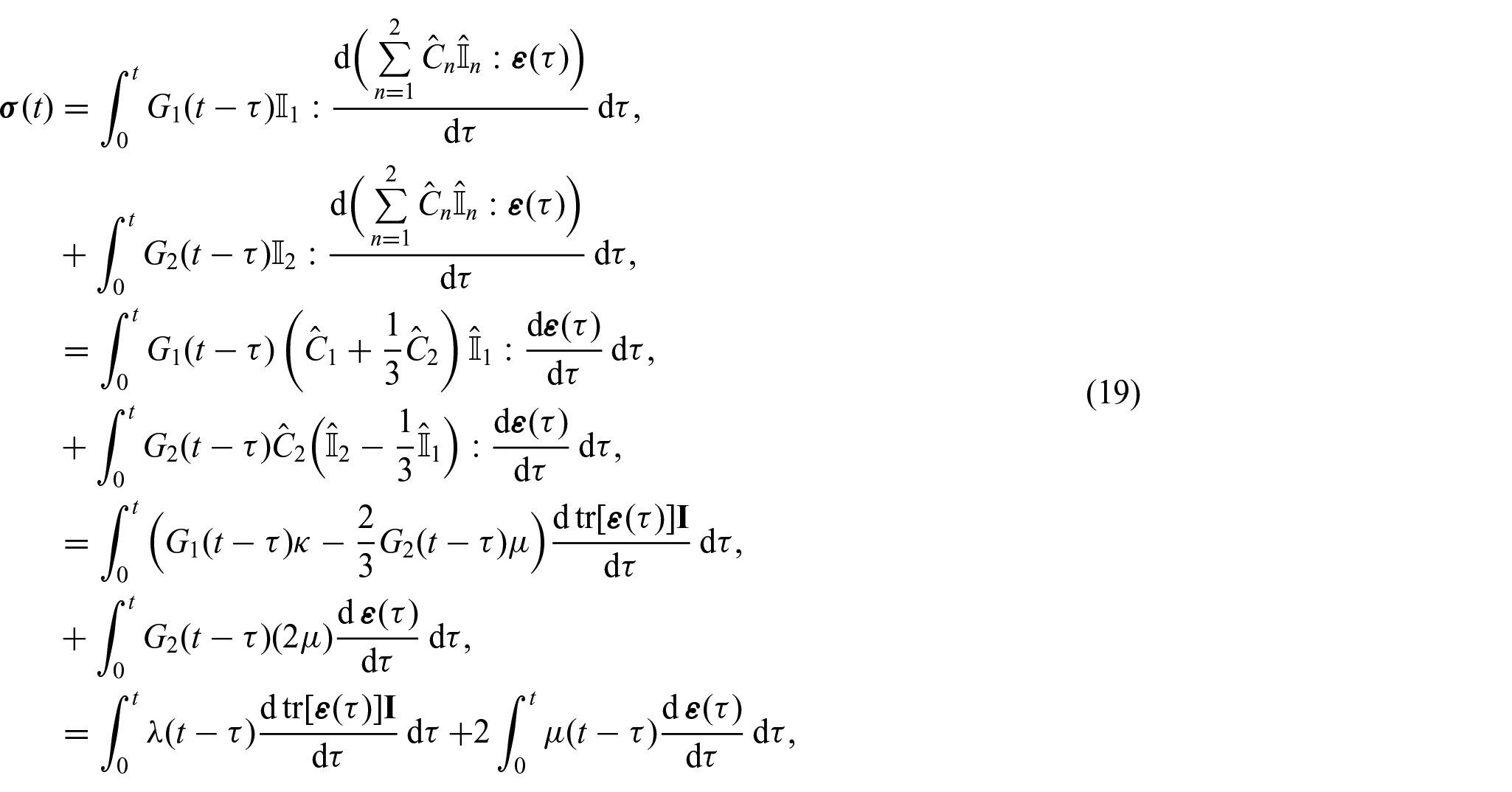
Similarly, we can obtain an equivalent form for $\mathbf{\sigma }$ using the set of bases in equation (5) to split the tensor $\mathbb{G}$ and the set of bases in equation (11) to write ${\mathbf{\sigma }}^{\mathrm{e}}$ , as follows:

$$\begin{array}{c}\mathbf{\sigma }(t)={\int }_0^t{G}_1(t-\tau ){\mathbb{I}}_1:\frac{\mathrm{d}(\sum _{n=1}^2{\hat{C}}_n{\hat{\mathbb{I}}}_n:\mathit{\epsilon }(\tau ))}{\mathrm{d}\tau }\mathrm{d}\tau ,\hfill \\ \multicolumn{1}{c}{+{\int }_0^t{G}_2(t-\tau ){\mathbb{I}}_2:\frac{\mathrm{d}(\sum _{n=1}^2{\hat{C}}_n{\hat{\mathbb{I}}}_n:\mathit{\epsilon }(\tau ))}{\mathrm{d}\tau }\mathrm{d}\tau ,}\\ \multicolumn{1}{c}{={\int }_0^t{G}_1(t-\tau )({\hat{C}}_1+\frac{1}{3}{\hat{C}}_2){\hat{\mathbb{I}}}_1:\frac{\mathrm{d}\mathit{\epsilon }(\tau )}{\mathrm{d}\tau }\mathrm{d}\tau ,}\\ \multicolumn{1}{c}{+{\int }_0^t{G}_2(t-\tau ){\hat{C}}_2({\hat{\mathbb{I}}}_2-\frac{1}{3}{\hat{\mathbb{I}}}_1):\frac{\mathrm{d}\mathit{\epsilon }(\tau )}{\mathrm{d}\tau }\mathrm{d}\tau ,}\\ \multicolumn{1}{c}{={\int }_0^t(G_1(t-\tau )\kappa -\frac{2}{3}{G}_2(t-\tau )\mu )\frac{\mathrm{d}\mathrm{tr}[\mathit{\epsilon }(\tau )]\mathbf{I}}{\mathrm{d}\tau }\mathrm{d}\tau ,}\\ \multicolumn{1}{c}{+{\int }_0^t{G}_2(t-\tau )(2\mu )\frac{\mathrm{d}\mathit{\epsilon }(\tau )}{\mathrm{d}\tau }\mathrm{d}\tau ,}\\ \multicolumn{1}{c}{={\int }_0^t\lambda (t-\tau )\frac{\mathrm{d}\mathrm{tr}[\mathit{\epsilon }(\tau )]\mathbf{I}}{\mathrm{d}\tau }\mathrm{d}\tau +2{\int }_0^t\mu (t-\tau )\frac{\mathrm{d}\mathit{\epsilon }(\tau )}{\mathrm{d}\tau }\mathrm{d}\tau ,}\end{array}$$

(19)

where we used the links between ${\hat{C}}_n$ and $C_n$ , $n=\{1,2\}$ in equations (13) and (18) and the results:

$${\mathbb{I}}_1:{\hat{\mathbb{I}}}_1={\hat{\mathbb{I}}}_1:{\mathbb{I}}_1={\hat{\mathbb{I}}}_1,{\mathbb{I}}_1:{\hat{\mathbb{I}}}_2={\hat{\mathbb{I}}}_2:{\mathbb{I}}_1=1/3{\hat{\mathbb{I}}}_1,$$

(20)

$${\mathbb{I}}_2:{\hat{\mathbb{I}}}_1={\hat{\mathbb{I}}}_1:{\mathbb{I}}_2=\mathbb{O},{\mathbb{I}}_2:{\hat{\mathbb{I}}}_2={\hat{\mathbb{I}}}_2:{\mathbb{I}}_2={\hat{\mathbb{I}}}_2-1/3{\hat{\mathbb{I}}}_1.$$

(21)

By comparing equation (17) with equation (19), we obtain the link between the relaxation function $\kappa (t)$ associated with the bulk modulus and the relaxation function $\lambda (t)$ associated with the first Lamé parameter: $\lambda (t)=\kappa (t)-\frac{2}{3}\mu (t),\forall t$ .

Finally, we note that, since the bases in equation (11) are not symmetrically additive, we cannot use them to split the tensor $\mathbb{G}$ . Indeed, they cannot be used to derive either of the two constitutive equations in equations (17) and (19).

2.2. How to obtain a symmetrically additive set of bases from a non-symmetrically additive set

Now, the question of whether it is possible to derive a set of symmetrically additive bases from a set of non-symmetrically additive bases arises naturally from the analysis carried out in the previous sections. We show here a simple method that works for the isotropic case, and in the next section, we will extend it to give a more general method that can be applied to anisotropic fourth-order tensors.

The problem can be stated as follows. Given a set of non-symmetrically additive isotropic bases $\{{\hat{\mathbb{K}}}_1,{\hat{\mathbb{K}}}_2\}$ , the requirement is to find a set of symmetrically additive isotropic bases $\{{\mathbb{K}}_1,{\mathbb{K}}_2\}$ , such that ${\mathbb{K}}_1+{\mathbb{K}}_2=\mathbb{S}$ .

Method 1. We first write the symmetrically additive bases as a linear combination of the non-symmetrically additive bases $\{{\hat{\mathbb{K}}}_1,{\hat{\mathbb{K}}}_2\}$ as follows:

$$\{\begin{array}{c}{\mathbb{K}}_1=a_{11}{\hat{\mathbb{K}}}_1+a_{12}{\hat{\mathbb{K}}}_2,\hfill \\ \multicolumn{1}{c}{{\mathbb{K}}_2=a_{21}{\hat{\mathbb{K}}}_1+a_{22}{\hat{\mathbb{K}}}_2.}\end{array}$$

(22)

Then, we impose the additive symmetry property by requiring that:

$$\underset{{\mathbb{K}}_1}{\underbrace{(a_{11}+a_{21}){\hat{\mathbb{K}}}_1}}+\underset{{\mathbb{K}}_2}{\underbrace{(a_{12}+a_{22}){\hat{\mathbb{K}}}_2}}-\mathbb{S}=\mathbb{O},$$

(23)

and we solve equation (23) to obtain the coefficients $a_{\mathrm{ij}}$ .

To illustrate Method 1, we derive a symmetrically additive set of bases from the bases $\{{\hat{\mathbb{I}}}_1,{\hat{\mathbb{I}}}_2\}$ in equation (11). The tensors ${\hat{\mathbb{I}}}_1,{\hat{\mathbb{I}}}_2$ , and $\mathbb{S}$ all share the symmetries in equation (76); therefore, equation (23) reduces to the following two equations:

$$\{\begin{array}{c}{a}_{11}+a_{21}=0,\hfill \\ \multicolumn{1}{c}{a_{12}+a_{22}=1.}\end{array}$$

(24)

Since the number of unknowns is greater than the number of equations, there are infinite solutions to the system in equation (24), namely, $a_{21}=-a_{11}$ and $a_{22}=1-a_{12}$ . However, we can use Properties (81) and (82) to restrict further the number of solutions and require that:

$${\mathbb{K}}_1:{\mathbb{K}}_1={\mathbb{K}}_1\iff a_{11}^2{\hat{\mathbb{I}}}_1:{\hat{\mathbb{I}}}_1+2a_{11}{a}_{12}{\hat{\mathbb{I}}}_1:{\hat{\mathbb{I}}}_2+a_{12}^2{\hat{\mathbb{I}}}_2:{\hat{\mathbb{I}}}_2=a_{11}{\hat{\mathbb{I}}}_1+a_{12}{\hat{\mathbb{I}}}_2,$$

(25)

$${\mathbb{K}}_2:{\mathbb{K}}_2={\mathbb{K}}_2\iff a_{21}^2{\hat{\mathbb{I}}}_1:{\hat{\mathbb{I}}}_1+2a_{21}{a}_{22}{\hat{\mathbb{I}}}_1:{\hat{\mathbb{I}}}_2+a_{22}^2{\hat{\mathbb{I}}}_2:{\hat{\mathbb{I}}}_2=a_{21}{\hat{\mathbb{I}}}_1+a_{22}{\hat{\mathbb{I}}}_2,$$

(26)

and

$${\mathbb{K}}_1:{\mathbb{K}}_2=\mathbb{O}\iff a_{11}{a}_{21}{\hat{\mathbb{I}}}_1:{\hat{\mathbb{I}}}_1+(a_{11}{a}_{22}+a_{12}{a}_{21}){\hat{\mathbb{I}}}_1:{\hat{\mathbb{I}}}_2+a_{12}{a}_{22}{\hat{\mathbb{I}}}_2:{\hat{\mathbb{I}}}_2=\mathbb{O},$$

(27)

respectively. Each of equations (25) and (26) reduce to a non-linear system of two equations in the following form:

$$\{\begin{array}{c}{a}_{11}(3a_{11}+2a_{12}-1)=0,\hfill \\ \multicolumn{1}{c}{a_{12}(a_{12}-1)=0,}\end{array}\mathrm{and}\{\begin{array}{c}{a}_{21}(3a_{21}+2a_{22}-1)=0,\hfill \\ \multicolumn{1}{c}{a_{22}(a_{22}-1)=0,}\end{array}$$

(28)

respectively. Equation (27) reduces to the following non-linear system:

$$\{\begin{array}{c}{a}_{12}{a}_{21}+a_{11}(3a_{21}+a_{22})=0\hfill \\ \multicolumn{1}{c}{a_{12}{a}_{22}=0.}\end{array}$$

(29)

By combining equation (24) with the first system of equation (28), we obtain the second system of equation (28), and vice-versa by combining equation (24) with the second system of equation (28), we obtain the first system in equation (28). Therefore, under the additive symmetry property, if one of the bases is idempotent, then the other is as well. Moreover, by combining equation (24) with equation (29), we obtain the second system in equation (28). Therefore, if the bases are orthogonal, then they are also idempotent and vice-versa. The systems in equations (24), (28), and (29) have the following four sets of solutions:

$$\mathbf{Sol}\mathbf{-}1\mathbf{:}{a}_{11}=a_{12}=a_{21}=0,a_{22}=1,$$

(30)

$$\mathbf{Sol}\mathbf{-}2\mathbf{:}{a}_{11}=a_{21}=a_{22}=0,a_{12}=1,$$

(31)

$$\mathbf{Sol}\mathbf{-}3\mathbf{:}{a}_{11}=-\frac{1}{3},a_{12}=1,a_{21}=\frac{1}{3},a_{22}=0,$$

(32)

$$\mathbf{Sol}\mathbf{-}4\mathbf{:}{a}_{11}=\frac{1}{3},a_{12}=0,a_{21}=-\frac{1}{3},a_{22}=1.$$

(33)

Sol-1 and Sol-2 can be discarded as they result in one of the two bases being zero. Sol-3 and Sol-4 are equivalent and give the symmetrically additive set in equation (5) which is also idempotent and orthogonal.

In conclusion, in this section, we have proposed a simple method for deriving a set of symmetrically additive bases from a non-symmetrically additive set for isotropic tensors. The method requires us to express the unknown symmetrically additive set as a linear combination of the known non-symmetrically additive bases and calculate the linear coefficients by imposing Property (3). As expected, there are infinite combinations of bases that satisfy the symmetrically additive property; however, there is only one set (given by Sol-3 and Sol-4 in equations (32) and (33)) that is both idempotent (Property (1)) and orthogonal (Property (2)).

We now investigate how this procedure can be extended to the anisotropic case. In particular, we show that Method 1 is not sufficient in this case, and an alternative route is required to construct a set of basis that is symmetrically additive.

3. Fourth-order bases for TI materials

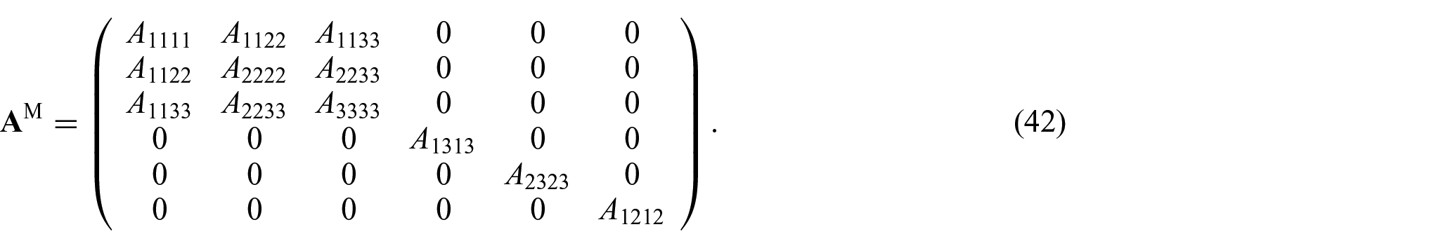
Let us now focus on TI materials. Such anisotropic materials typically either contain a family of fibres or a layered structure that produces mechanical behaviour along a single axis that is distinct from that in the transverse directions. We identify this preferred direction with the unit vector $\mathbf{m}$ , which, for brevity, we call the fibre vector. The elasticity tensor ${\mathbb{C}}^{\mathrm{TI}}$ for a TI material has six components, of which five are independent due to its symmetries.

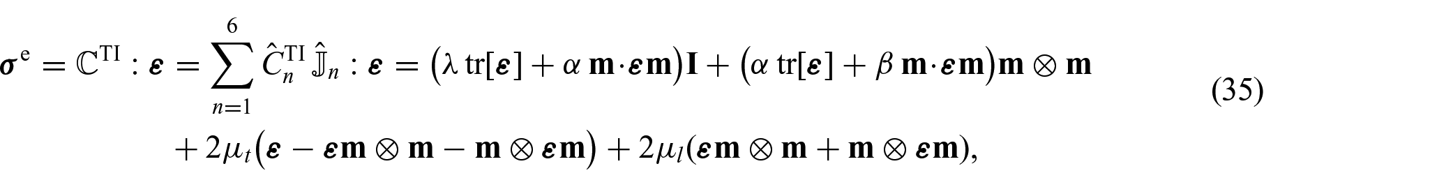
As in the previous section, we start by writing the constitutive equation for a linear elastic material, but now in the case of transverse isotropy. The following set of bases was originally proposed by Spencer [10]:

$$\begin{array}{c}{\hat{\mathbb{J}}}_1=\mathbf{I}\otimes \mathbf{I},{\hat{\mathbb{J}}}_2=\mathbf{I}\otimes (\mathbf{m}\otimes \mathbf{m}),{\hat{\mathbb{J}}}_3=(\mathbf{m}\otimes \mathbf{m})\otimes \mathbf{I},{\hat{\mathbb{J}}}_4=(\mathbf{m}\otimes \mathbf{m})\otimes (\mathbf{m}\otimes \mathbf{m}),\hfill \\ \multicolumn{1}{c}{{\hat{\mathbb{J}}}_5=\frac{1}{2}(\overline{\mathbb{I}}+\underset{¯}{\mathbb{I}})-\frac{1}{2}(\mathbf{I}\overline{\otimes }(\mathbf{m}\otimes \mathbf{m})+\mathbf{I}\underset{¯}{\otimes }(\mathbf{m}\otimes \mathbf{m})+(\mathbf{m}\otimes \mathbf{m})\overline{\otimes }\mathbf{I}+(\mathbf{m}\otimes \mathbf{m})\underset{¯}{\otimes }\mathbf{I}),}\\ \multicolumn{1}{c}{{\hat{\mathbb{J}}}_6=\frac{1}{2}(\overline{\mathbb{I}}+\underset{¯}{\mathbb{I}})-{\hat{\mathbb{J}}}_5,}\end{array}$$

(34)

and yields to the well-known form:

$$\begin{array}{c}{\mathbf{\sigma }}^{\mathrm{e}}={\mathbb{C}}^{\mathrm{TI}}:\mathit{\epsilon }=\sum _{n=1}^6{\hat{C}}_n^{\mathrm{TI}}{\hat{\mathbb{J}}}_n:\mathit{\epsilon }=(\lambda \mathrm{tr}[\mathit{\epsilon }]+\alpha \mathbf{m}·\mathit{\epsilon }\mathbf{m})\mathbf{I}+(\alpha \mathrm{tr}[\mathit{\epsilon }]+\beta \mathbf{m}·\mathit{\epsilon }\mathbf{m})\mathbf{m}\otimes \mathbf{m}\hfill \\ \multicolumn{1}{c}{+2{\mu }_t(\mathit{\epsilon }-\mathit{\epsilon }\mathbf{m}\otimes \mathbf{m}-\mathbf{m}\otimes \mathit{\epsilon }\mathbf{m})+2{\mu }_l(\mathit{\epsilon }\mathbf{m}\otimes \mathbf{m}+\mathbf{m}\otimes \mathit{\epsilon }\mathbf{m}),}\end{array}$$

(35)

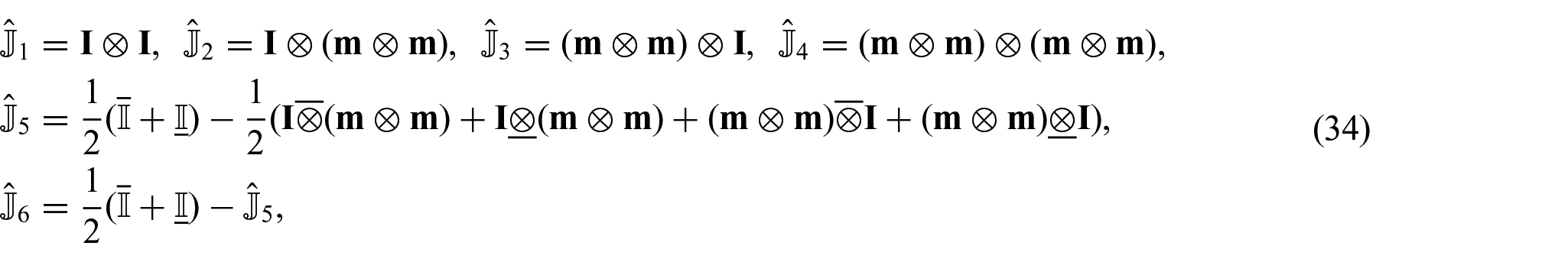
where ${\mu }_t$ and ${\mu }_l$ are the shear moduli associated with shear in the plane of isotropy and the planes containing the axis of anisotropy, respectively, and $\alpha$ and $\beta$ are the two parameters related to Young’s moduli of the isotropic matrix and the fibres, respectively. Another set of TI bases that is commonly used in the continuum mechanics community is given by the Hill bases [16, 17]:

$$\begin{array}{c}{\hat{\mathbb{H}}}_1=\frac{1}{2}\mathbf{\Theta }\otimes \mathbf{\Theta },{\hat{\mathbb{H}}}_2=\mathbf{\Theta }\otimes (\mathbf{m}\otimes \mathbf{m}),{\hat{\mathbb{H}}}_3=(\mathbf{m}\otimes \mathbf{m})\otimes \mathbf{\Theta },\hfill \\ \multicolumn{1}{c}{{\hat{\mathbb{H}}}_4=\mathbf{m}\otimes \mathbf{m}\otimes \mathbf{m}\otimes \mathbf{m}{\hat{\mathbb{H}}}_5=\frac{1}{2}(\mathbf{\Theta }\overline{\otimes }\mathbf{\Theta }+\mathbf{\Theta }\underset{¯}{\otimes }\mathbf{\Theta }-\mathbf{\Theta }\otimes \mathbf{\Theta }),}\\ \multicolumn{1}{c}{{\hat{\mathbb{H}}}_6=\frac{1}{2}(\mathbf{\Theta }\overline{\otimes }(\mathbf{m}\otimes \mathbf{m})+\mathbf{\Theta }\underset{¯}{\otimes }(\mathbf{m}\otimes \mathbf{m})+(\mathbf{m}\otimes \mathbf{m})\overline{\otimes }\mathbf{\Theta }+(\mathbf{m}\otimes \mathbf{m})\underset{¯}{\otimes }\mathbf{\Theta }),}\end{array}$$

(36)

where $\mathbf{\Theta }=\mathbf{I}-\mathbf{m}\otimes \mathbf{m}$ . We can easily verify that both the bases in equations (34) and (36) are not symmetrically additive. As opposed to the isotropic case, a symmetrically additive set of bases for TI tensors has not yet been proposed in the literature. Our aim here is to construct such a set together with a general method for deriving a symmetrically additive set of bases for TI tensors. Method 1 is easy to implement in the isotropic case, where the number of unknowns, i.e., the four coefficients in equation (22), is small. However, in the TI case, Method 1 would lead us to state the problem as follows. Given a set of non-symmetrically additive TI bases $\{{\hat{\mathbb{K}}}_1,\dots ,{\hat{\mathbb{K}}}_6\}$ , we require to find a set of symmetrically additive TI bases $\{{\mathbb{K}}_1,\dots ,{\mathbb{K}}_6\}$ as a linear combination of $\{{\hat{\mathbb{K}}}_1,\dots ,{\hat{\mathbb{K}}}_6\}$ :

$${\mathbb{K}}_i=\sum _{n=1}^6{a}_{\mathrm{in}}{\hat{\mathbb{K}}}_n\mathrm{for}i=\{1,\dots ,6\},$$

(37)

such that:

$$\sum _{n=1}^6{\mathbb{K}}_n=\sum _{n=1}^6\sum _{i=1}^6{a}_{\mathrm{in}}{\hat{\mathbb{K}}}_n=\mathbb{S}.$$

(38)

From equation (37), we know that now the problem has 36 unknowns, i.e., the coefficients $a_{\mathrm{in}}$ (with $i,n=\{1,\dots ,6\}$ ), and from equation (38), we obtain only 7 equations. The number of equations follows from the symmetries of the TI tensors. Indeed, the TI bases ${\hat{\mathbb{K}}}_n$ have only the minor symmetries (see equation (76) in section 2). Therefore, the seven equations can be obtained from the components $\{1111\},\{1122\},\{1133\},\{3311\},\{3333\},\{1212\}$ , and $\{1313\}$ of equation (38). To obtain the remaining equations, we cannot impose idempotence and orthogonality since for TI tensors, these two properties are incompatible, meaning that a set of TI bases cannot be simultaneously idempotent and orthogonal. The main conclusion here is: Method 1 only tells us that for TI tensors there are infinitely many symmetrically additive sets of bases that are a linear combination of a non-symmetrically additive set; however, Method 1 does not yield any explicit expression. We therefore construct the following alternative method.

Method 2. We first write the symmetrically additive bases as follows:

$${\mathbb{K}}_n=\mathbb{A}:{\hat{\mathbb{K}}}_n,$$

(39)

where $\mathbb{A}$ is a fourth-order tensor whose entries are unknown coefficients to be determined. We then impose the additive symmetry property on the bases ${\mathbb{K}}_n$ by requiring that:

$$\sum _{n=1}^6{\mathbb{K}}_n=\mathbb{A}:\left(\sum _{n=1}^6{\hat{\mathbb{K}}}_n\right)=\mathbb{S}.$$

(40)

Since $\mathbb{S}$ is the fourth-order symmetric identity tensor, it follows from equation (40) that:

$$\mathbb{A}={\left(\sum _{n=1}^6{\hat{\mathbb{K}}}_n\right)}^{-1}.$$

(41)

Therefore, $\mathbb{A}$ is the inverse of the tensor $\sum _{n=1}^6{\hat{\mathbb{K}}}_n$ .

Now, if all the six bases ${\hat{\mathbb{K}}}_n$ have the minor symmetries of the tensor $\mathbb{S}$ , the tensor given by the sum of the bases also has these symmetries, and therefore, it is possible to convert it into a $6\times 6$ symmetric matrix ${\mathbf{A}}^{\mathrm{M}}$ , which, according to the Mandel–Voigt notation [18], has the following components:

$${\mathbf{A}}^{\mathrm{M}}=\left(\begin{array}{cccccc}{A}_{1111}\hfill & A_{1122}\hfill & A_{1133}\hfill & 0\hfill & 0\hfill & 0\hfill \\ \multicolumn{1}{c}{A_{1122}}& A_{2222}\hfill & A_{2233}\hfill & 0\hfill & 0\hfill & 0\hfill \\ \multicolumn{1}{c}{A_{1133}}& A_{2233}\hfill & A_{3333}\hfill & 0\hfill & 0\hfill & 0\hfill \\ \multicolumn{1}{c}{0}& 0\hfill & 0\hfill & A_{1313}\hfill & 0\hfill & 0\hfill \\ \multicolumn{1}{c}{0}& 0\hfill & 0\hfill & 0\hfill & A_{2323}\hfill & 0\hfill \\ \multicolumn{1}{c}{0}& 0\hfill & 0\hfill & 0\hfill & 0\hfill & A_{1212}\hfill \end{array}\right).$$

(42)

We note that, in order to be invertible, a symmetric matrix needs to be positive definite. We omit the proof here; however, it is possible to show that this is true for all TI tensors ${\hat{\mathbb{K}}}_n$ . Moreover, the matrix ${\mathbf{A}}^{\mathrm{M}}$ is unique. This does not mean that there is only one set of symmetrically additive bases that can be derived from a given set of non-symmetrically additive bases; indeed, as discussed above, there is an infinite number. However, we are not interested in finding a specific set, as long as it satisfies the property of additive symmetry.

3.1. Example 1: Hill bases

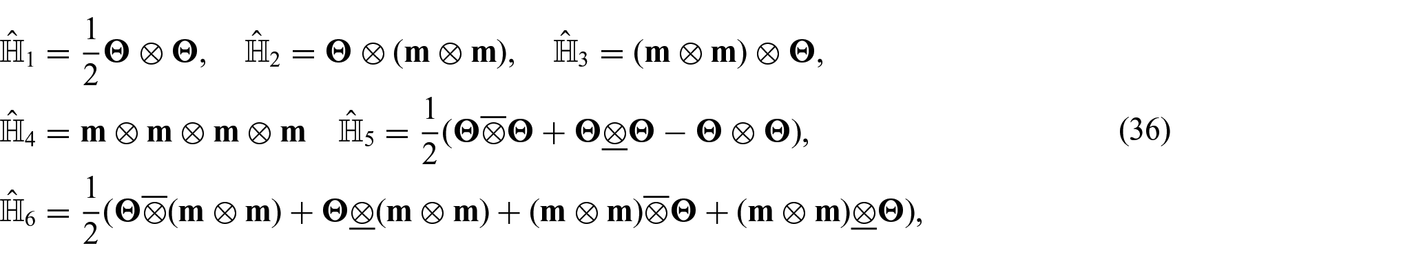
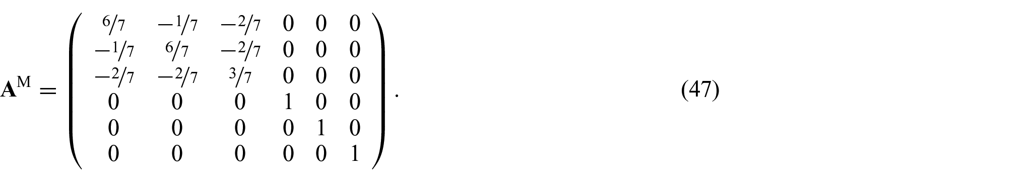
We now apply Method 2 to obtain a symmetrically additive set of TI bases from the Hill bases in equation (36). To simplify the calculations, we consider the fibres to be aligned with the vector $\mathbf{m}=(0,0,1{)}^{\mathrm{T}}$ . We take the fibre vector to be one of the reference axes in 3D Euclidean space. The fibre vector $\mathbf{m}$ is a unit vector. Moreover, in the small deformation setting, the vector $\mathbf{m}$ is independent of the deformation. We first obtain the tensor $\mathbb{A}$ which is given by:

$$\mathbb{A}={\left(\sum _{n=1}^6{\hat{\mathbb{H}}}_n\right)}^{-1}={(\mathbb{S}+\mathbf{\Theta }\otimes \mathbf{m}\otimes \mathbf{m}+\mathbf{m}\otimes \mathbf{m}\otimes \mathbf{\Theta })}^{-1}.$$

(43)

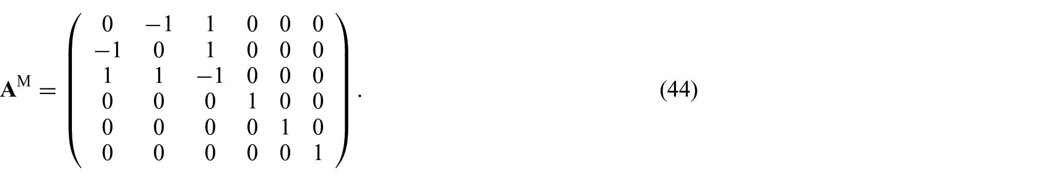
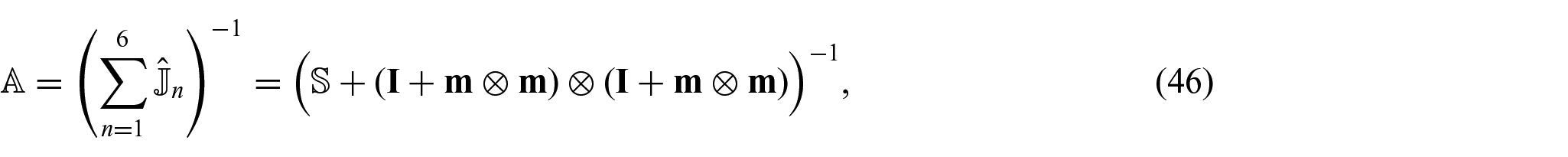
To calculate the inverse, we convert the tensor on the right of equation (43) into its Mandel–Voigt form. Then, we invert the $6\times 6$ symmetric matrix. The result is:

$${\mathbf{A}}^{\mathrm{M}}=\left(\begin{array}{cccccc}0\hfill & -1\hfill & 1\hfill & 0\hfill & 0\hfill & 0\hfill \\ \multicolumn{1}{c}{-1}& 0\hfill & 1\hfill & 0\hfill & 0\hfill & 0\hfill \\ \multicolumn{1}{c}{1}& 1\hfill & -1\hfill & 0\hfill & 0\hfill & 0\hfill \\ \multicolumn{1}{c}{0}& 0\hfill & 0\hfill & 1\hfill & 0\hfill & 0\hfill \\ \multicolumn{1}{c}{0}& 0\hfill & 0\hfill & 0\hfill & 1\hfill & 0\hfill \\ \multicolumn{1}{c}{0}& 0\hfill & 0\hfill & 0\hfill & 0\hfill & 1\hfill \end{array}\right).$$

(44)

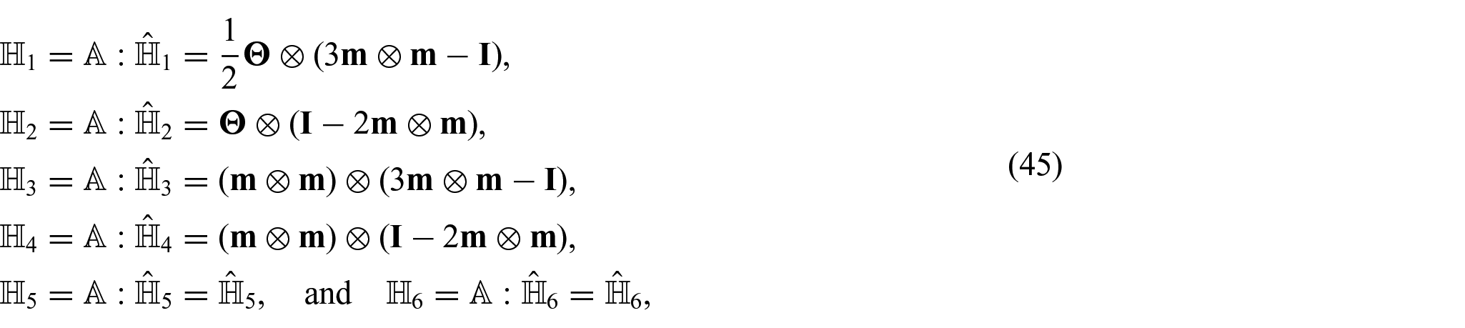
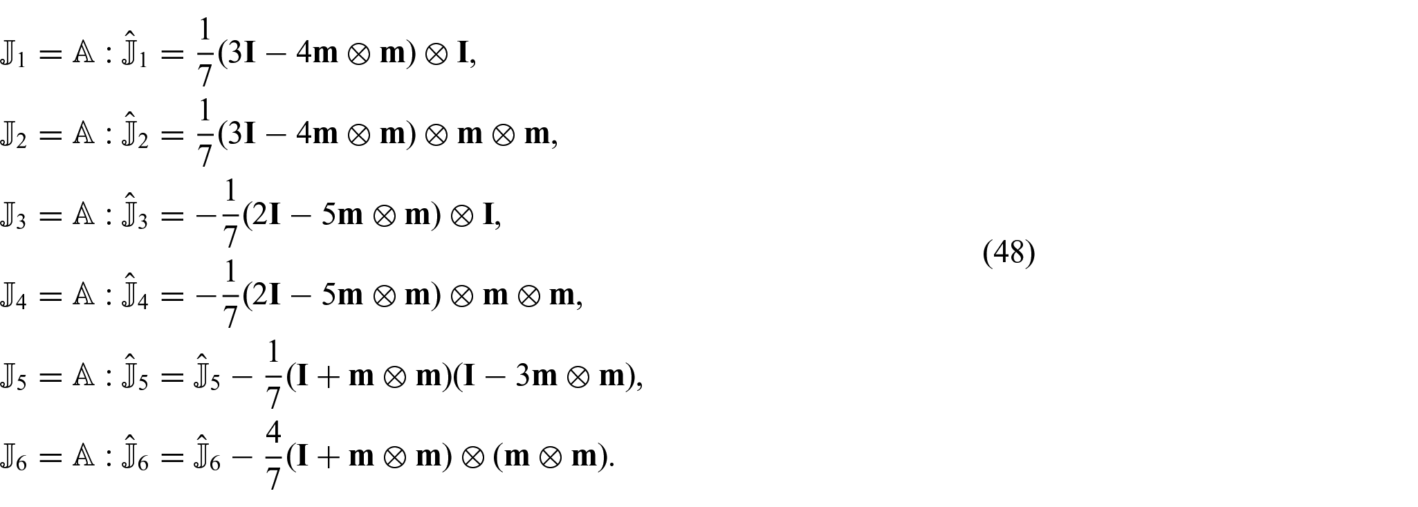
We can now revert the matrix ${\mathbf{A}}^{\mathrm{M}}$ into a fourth-order tensor and calculate the symmetrically additive bases using equation (39):

$$\begin{array}{c}{\mathbb{H}}_1=\mathbb{A}:{\hat{\mathbb{H}}}_1=\frac{1}{2}\mathbf{\Theta }\otimes (3\mathbf{m}\otimes \mathbf{m}-\mathbf{I}),\hfill \\ \multicolumn{1}{c}{{\mathbb{H}}_2=\mathbb{A}:{\hat{\mathbb{H}}}_2=\mathbf{\Theta }\otimes (\mathbf{I}-2\mathbf{m}\otimes \mathbf{m}),}\\ \multicolumn{1}{c}{{\mathbb{H}}_3=\mathbb{A}:{\hat{\mathbb{H}}}_3=(\mathbf{m}\otimes \mathbf{m})\otimes (3\mathbf{m}\otimes \mathbf{m}-\mathbf{I}),}\\ \multicolumn{1}{c}{{\mathbb{H}}_4=\mathbb{A}:{\hat{\mathbb{H}}}_4=(\mathbf{m}\otimes \mathbf{m})\otimes (\mathbf{I}-2\mathbf{m}\otimes \mathbf{m}),}\\ \multicolumn{1}{c}{{\mathbb{H}}_5=\mathbb{A}:{\hat{\mathbb{H}}}_5={\hat{\mathbb{H}}}_5,\mathrm{and}{\mathbb{H}}_6=\mathbb{A}:{\hat{\mathbb{H}}}_6={\hat{\mathbb{H}}}_6,}\end{array}$$

(45)

where now $\sum _{n=1}^6{\mathbb{H}}_n=\mathbb{S}$ . The split in equation (45) is valid for any unit vector $\mathbf{m}$ . We only used the specific case $\mathbf{m}={\mathbf{e}}_3$ to simplify the algebraic calculations.

3.2. Example 2: Spencer bases

We now consider the set of bases proposed by Spencer. This set leads to a formulation of the constitutive equation which is frequently used in the literature and makes use of constitutive parameters which are easily measurable experimentally. The tensor $\mathbb{A}$ for the Spencer set is given by:

$$\mathbb{A}={\left(\sum _{n=1}^6{\hat{\mathbb{J}}}_n\right)}^{-1}=(\mathbb{S}+(\mathbf{I}+\mathbf{m}\otimes \mathbf{m})\otimes (\mathbf{I}+\mathbf{m}\otimes \mathbf{m}){)}^{-1},$$

(46)

which can be written in the following Mandel–Voigt form:

$${\mathbf{A}}^{\mathrm{M}}=\left(\begin{array}{cccccc}6/7\hfill & -1/7\hfill & -2/7\hfill & 0\hfill & 0\hfill & 0\hfill \\ \multicolumn{1}{c}{-1/7}& 6/7\hfill & -2/7\hfill & 0\hfill & 0\hfill & 0\hfill \\ \multicolumn{1}{c}{-2/7}& -2/7\hfill & 3/7\hfill & 0\hfill & 0\hfill & 0\hfill \\ \multicolumn{1}{c}{0}& 0\hfill & 0\hfill & 1\hfill & 0\hfill & 0\hfill \\ \multicolumn{1}{c}{0}& 0\hfill & 0\hfill & 0\hfill & 1\hfill & 0\hfill \\ \multicolumn{1}{c}{0}& 0\hfill & 0\hfill & 0\hfill & 0\hfill & 1\hfill \end{array}\right).$$

(47)

The symmetrically additive set is then given by:

$$\begin{array}{c}{\mathbb{J}}_1=\mathbb{A}:{\hat{\mathbb{J}}}_1=\frac{1}{7}(3\mathbf{I}-4\mathbf{m}\otimes \mathbf{m})\otimes \mathbf{I},\hfill \\ \multicolumn{1}{c}{{\mathbb{J}}_2=\mathbb{A}:{\hat{\mathbb{J}}}_2=\frac{1}{7}(3\mathbf{I}-4\mathbf{m}\otimes \mathbf{m})\otimes \mathbf{m}\otimes \mathbf{m},}\\ \multicolumn{1}{c}{{\mathbb{J}}_3=\mathbb{A}:{\hat{\mathbb{J}}}_3=-\frac{1}{7}(2\mathbf{I}-5\mathbf{m}\otimes \mathbf{m})\otimes \mathbf{I},}\\ \multicolumn{1}{c}{{\mathbb{J}}_4=\mathbb{A}:{\hat{\mathbb{J}}}_4=-\frac{1}{7}(2\mathbf{I}-5\mathbf{m}\otimes \mathbf{m})\otimes \mathbf{m}\otimes \mathbf{m},}\\ \multicolumn{1}{c}{{\mathbb{J}}_5=\mathbb{A}:{\hat{\mathbb{J}}}_5={\hat{\mathbb{J}}}_5-\frac{1}{7}(\mathbf{I}+\mathbf{m}\otimes \mathbf{m})(\mathbf{I}-3\mathbf{m}\otimes \mathbf{m}),}\\ \multicolumn{1}{c}{{\mathbb{J}}_6=\mathbb{A}:{\hat{\mathbb{J}}}_6={\hat{\mathbb{J}}}_6-\frac{4}{7}(\mathbf{I}+\mathbf{m}\otimes \mathbf{m})\otimes (\mathbf{m}\otimes \mathbf{m}).}\end{array}$$

(48)

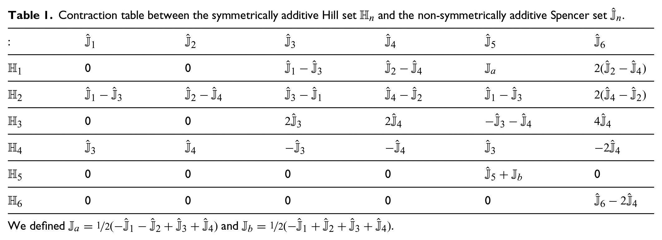
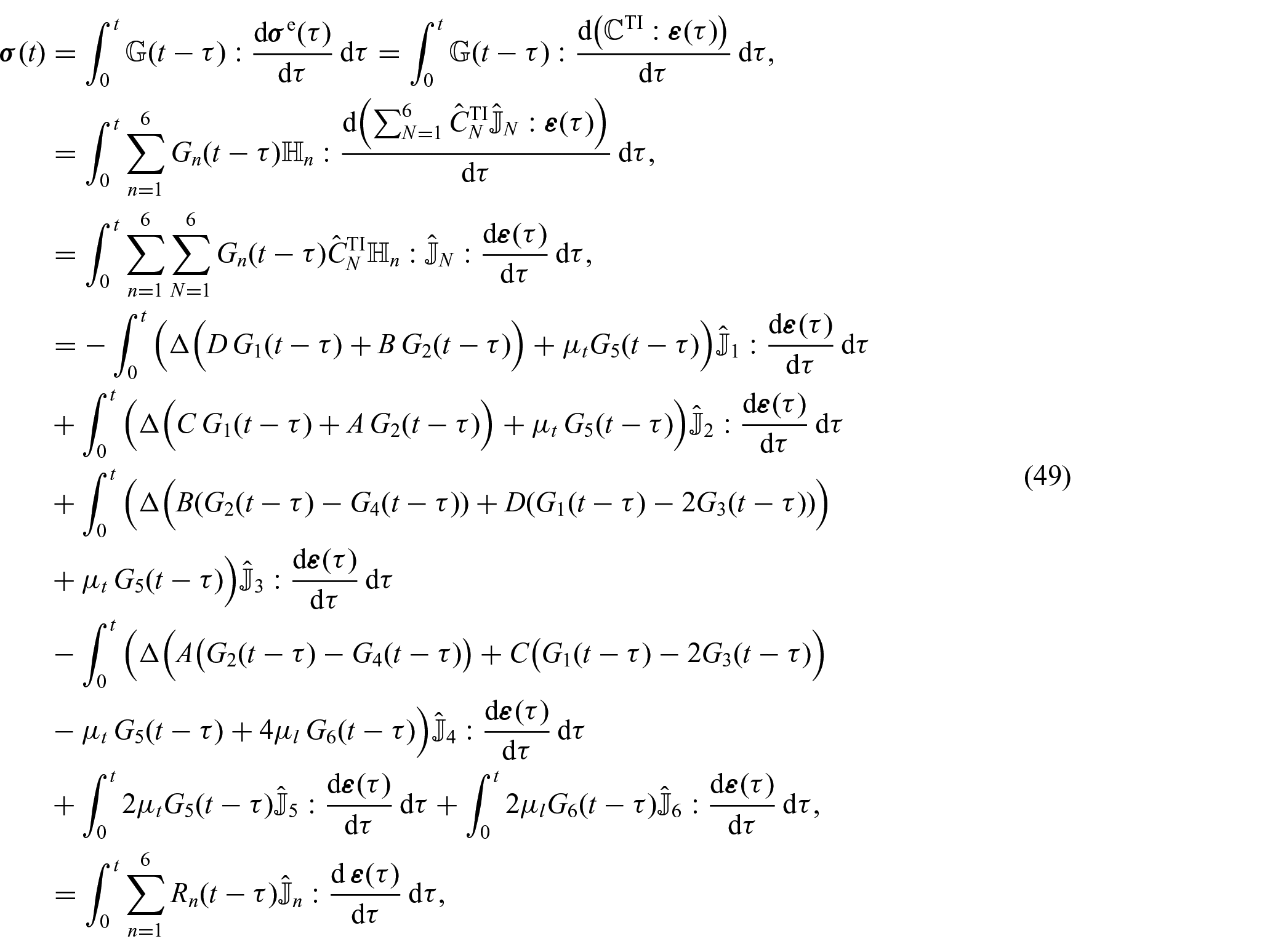
Let us now write down the constitutive equation for a TI linear viscoelastic material. We use the symmetrically additive set in equation (45) to split the relaxation tensor $\mathbb{G}$ and the Spencer set in equation (34) to write the elastic stress. This choice will allow us to simplify the calculations; however, we could alternatively use the symmetrically additive set in equation (48) to split $\mathbb{G}$ and to obtain the same constitutive equation. We leave this as exercise for the interested reader. By making use of the contraction products in Table 1,

Table 1.

Contraction table between the symmetrically additive Hill set ${\mathbb{H}}_n$ and the non-symmetrically additive Spencer set ${\hat{\mathbb{J}}}_n$ .

:	${\hat{\mathbb{J}}}_1$	${\hat{\mathbb{J}}}_2$	${\hat{\mathbb{J}}}_3$	${\hat{\mathbb{J}}}_4$	${\hat{\mathbb{J}}}_5$	${\hat{\mathbb{J}}}_6$
${\mathbb{H}}_1$	0	0	${\hat{\mathbb{J}}}_1-{\hat{\mathbb{J}}}_3$	${\hat{\mathbb{J}}}_2-{\hat{\mathbb{J}}}_4$	${\mathbb{J}}_a$	$2({\hat{\mathbb{J}}}_2-{\hat{\mathbb{J}}}_4)$
${\mathbb{H}}_2$	${\hat{\mathbb{J}}}_1-{\hat{\mathbb{J}}}_3$	${\hat{\mathbb{J}}}_2-{\hat{\mathbb{J}}}_4$	${\hat{\mathbb{J}}}_3-{\hat{\mathbb{J}}}_1$	${\hat{\mathbb{J}}}_4-{\hat{\mathbb{J}}}_2$	${\hat{\mathbb{J}}}_1-{\hat{\mathbb{J}}}_3$	$2({\hat{\mathbb{J}}}_4-{\hat{\mathbb{J}}}_2)$
${\mathbb{H}}_3$	0	0	$2{\hat{\mathbb{J}}}_3$	$2{\hat{\mathbb{J}}}_4$	$-{\hat{\mathbb{J}}}_3-{\hat{\mathbb{J}}}_4$	$4{\hat{\mathbb{J}}}_4$
${\mathbb{H}}_4$	${\hat{\mathbb{J}}}_3$	${\hat{\mathbb{J}}}_4$	$-{\hat{\mathbb{J}}}_3$	$-{\hat{\mathbb{J}}}_4$	${\hat{\mathbb{J}}}_3$	$-2{\hat{\mathbb{J}}}_4$
${\mathbb{H}}_5$	0	0	0	0	${\hat{\mathbb{J}}}_5+{\mathbb{J}}_b$	0
${\mathbb{H}}_6$	0	0	0	0	0	${\hat{\mathbb{J}}}_6-2{\hat{\mathbb{J}}}_4$

We defined ${\mathbb{J}}_a=1/2(-{\hat{\mathbb{J}}}_1-{\hat{\mathbb{J}}}_2+{\hat{\mathbb{J}}}_3+{\hat{\mathbb{J}}}_4)$ and ${\mathbb{J}}_b=1/2(-{\hat{\mathbb{J}}}_1+{\hat{\mathbb{J}}}_2+{\hat{\mathbb{J}}}_3+{\hat{\mathbb{J}}}_4)$ .

we obtain:

$$\begin{array}{c}\mathbf{\sigma }(t)={\int }_0^t\mathbb{G}(t-\tau ):\frac{\mathrm{d}{\mathbf{\sigma }}^{\mathrm{e}}(\tau )}{\mathrm{d}\tau }\mathrm{d}\tau ={\int }_0^t\mathbb{G}(t-\tau ):\frac{\mathrm{d}({\mathbb{C}}^{\mathrm{TI}}:\mathit{\epsilon }(\tau ))}{\mathrm{d}\tau }\mathrm{d}\tau ,\hfill \\ \multicolumn{1}{c}{={\int }_0^t\sum _{n=1}^6{G}_n(t-\tau ){\mathbb{H}}_n:\frac{\mathrm{d}(\sum _{N=1}^6{\hat{C}}_N^{\mathrm{TI}}{\hat{\mathbb{J}}}_N:\mathit{\epsilon }(\tau ))}{\mathrm{d}\tau }\mathrm{d}\tau ,}\\ \multicolumn{1}{c}{={\int }_0^t\sum _{n=1}^6\sum _{N=1}^6{G}_n(t-\tau ){\hat{C}}_N^{\mathrm{TI}}{\mathbb{H}}_n:{\hat{\mathbb{J}}}_N:\frac{\mathrm{d}\mathit{\epsilon }(\tau )}{\mathrm{d}\tau }\mathrm{d}\tau ,}\\ \multicolumn{1}{c}{=-{\int }_0^t(\mathrm{\Delta }(D{G}_1(t-\tau )+B{G}_2(t-\tau ))+{\mu }_t{G}_5(t-\tau )){\hat{\mathbb{J}}}_1:\frac{\mathrm{d}\mathit{\epsilon }(\tau )}{\mathrm{d}\tau }\mathrm{d}\tau }\\ \multicolumn{1}{c}{+{\int }_0^t(\mathrm{\Delta }(C{G}_1(t-\tau )+A{G}_2(t-\tau ))+{\mu }_t{G}_5(t-\tau )){\hat{\mathbb{J}}}_2:\frac{\mathrm{d}\mathit{\epsilon }(\tau )}{\mathrm{d}\tau }\mathrm{d}\tau }\\ \multicolumn{1}{c}{+{\int }_0^t(\mathrm{\Delta }(B(G_2(t-\tau )-G_4(t-\tau ))+D(G_1(t-\tau )-2G_3(t-\tau )))}\\ \multicolumn{1}{c}{+{\mu }_t{G}_5(t-\tau )){\hat{\mathbb{J}}}_3:\frac{\mathrm{d}\mathit{\epsilon }(\tau )}{\mathrm{d}\tau }\mathrm{d}\tau }\\ \multicolumn{1}{c}{-{\int }_0^t(\mathrm{\Delta }(A(G_2(t-\tau )-G_4(t-\tau ))+C(G_1(t-\tau )-2G_3(t-\tau ))}\\ \multicolumn{1}{c}{-{\mu }_t{G}_5(t-\tau )+4{\mu }_l{G}_6(t-\tau )){\hat{\mathbb{J}}}_4:\frac{\mathrm{d}\mathit{\epsilon }(\tau )}{\mathrm{d}\tau }\mathrm{d}\tau }\\ \multicolumn{1}{c}{+{\int }_0^{t}2{\mu }_t{G}_5(t-\tau ){\hat{\mathbb{J}}}_5:\frac{\mathrm{d}\mathit{\epsilon }(\tau )}{\mathrm{d}\tau }\mathrm{d}\tau +{\int }_0^{t}2{\mu }_l{G}_6(t-\tau ){\hat{\mathbb{J}}}_6:\frac{\mathrm{d}\mathit{\epsilon }(\tau )}{\mathrm{d}\tau }\mathrm{d}\tau ,}\\ \multicolumn{1}{c}{={\int }_0^t\sum _{n=1}^6{R}_n(t-\tau ){\hat{\mathbb{J}}}_n:\frac{\mathrm{d}\mathit{\epsilon }(\tau )}{\mathrm{d}\tau }\mathrm{d}\tau ,}\end{array}$$

(49)

where:

$$\begin{array}{c}A=\frac{1}{\mathrm{\Delta }}(\alpha -\beta -4{\mu }_L),B=\frac{1}{\mathrm{\Delta }}(\alpha -\lambda -2{\mu }_T),\hfill \\ \multicolumn{1}{c}{C=\frac{1}{\mathrm{\Delta }}(\beta +4{\mu }_L-{\mu }_T),D=\frac{1}{\mathrm{\Delta }}({\mu }_T-\alpha ),}\\ \multicolumn{1}{c}{\mathrm{\Delta }=(\alpha -\lambda -2{\mu }_T)(\beta +4{\mu }_L-{\mu }_T)-(\alpha -\beta -4{\mu }_L)({\mu }_T-\alpha ),}\end{array}$$

(50)

and

$$\begin{array}{c}{R}_1(t)=\lambda (t),R_2(t)=R_3(t)=\alpha (t),\hfill \\ \multicolumn{1}{c}{R_4(t)=\beta (t),R_5(t)=2{\mu }_t(t),R_6(t)=2{\mu }_l(t).}\end{array}$$

(51)

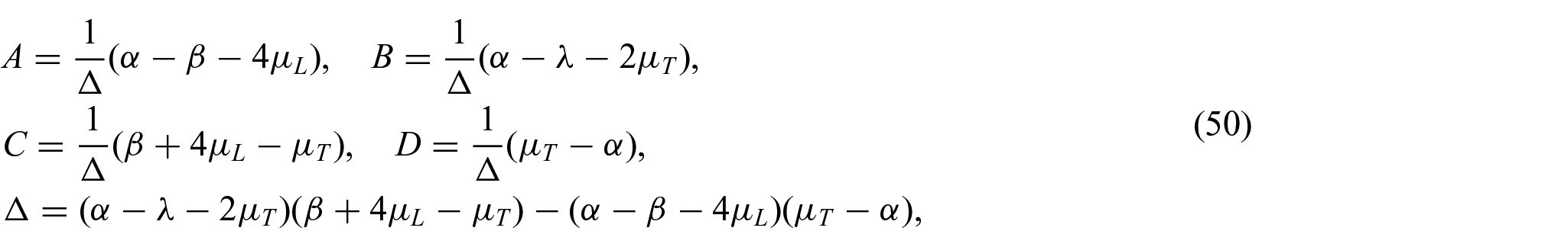
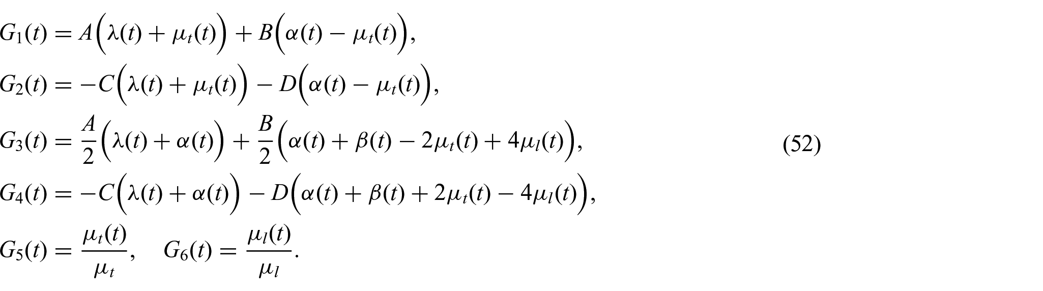
By comparing the last two equations in equation (49), we find the links between the reduced relaxation functions $G_n(t)$ and the time-dependent moduli $\lambda (t),\alpha (t),\beta (t),{\mu }_t(t)$ , and ${\mu }_l(t)$ , which are given by:

$$\begin{array}{c}{G}_1(t)=A(\lambda (t)+{\mu }_t(t))+B(\alpha (t)-{\mu }_t(t)),\hfill \\ \multicolumn{1}{c}{G_2(t)=-C(\lambda (t)+{\mu }_t(t))-D(\alpha (t)-{\mu }_t(t)),}\\ \multicolumn{1}{c}{G_3(t)=\frac{A}{2}(\lambda (t)+\alpha (t))+\frac{B}{2}(\alpha (t)+\beta (t)-2{\mu }_t(t)+4{\mu }_l(t)),}\\ \multicolumn{1}{c}{G_4(t)=-C(\lambda (t)+\alpha (t))-D(\alpha (t)+\beta (t)+2{\mu }_t(t)-4{\mu }_l(t)),}\\ \multicolumn{1}{c}{G_5(t)=\frac{{\mu }_t(t)}{{\mu }_t},G_6(t)=\frac{{\mu }_l(t)}{{\mu }_l}.}\end{array}$$

(52)

We note that to go from the third to the fourth equation in equation (49), we have used the fact that the bases are time-independent (they only depend on the fibres vector $\mathbf{m}$ , which in the small deformation regime is a unit vector and does not depend on the time nor the deformation).

The links in equation (52) allow us to find a connection between the functions $G_n(t)$ (associated with the symmetrically additive set of Hill bases $\mathbb{H}$ ) and the moduli $\lambda (t),\alpha (t),\beta (t),{\mu }_t(t),{\mu }_l(t)$ , which are associated with five physical modes of deformation, and therefore can be experimentally measured by performing a hydrostatic compression, a simple shear in the plane of isotropy, two simple shears in the planes perpendicular to the preferred direction, both parallel and perpendicular to the preferred direction, and a uni-axial tension.

To summarise the results of this section, we have now constructed a set of symmetrically additive bases to split the relaxation tensor $\mathbb{G}(t)$ for TI viscoelastic materials. In the next section, we will apply the symmetrically additive splits for isotropic and TI tensors to the context of MQLV. We will show that, in the large deformation regime, the bases depend on the deformation, and therefore, the relaxation tensor $\mathbb{G}$ is naturally deformation-dependent. We will illustrate this property with simple examples, by considering different deformation modes that are typically used in mechanical testing.

4. Modified quasi-linear viscoelasticity

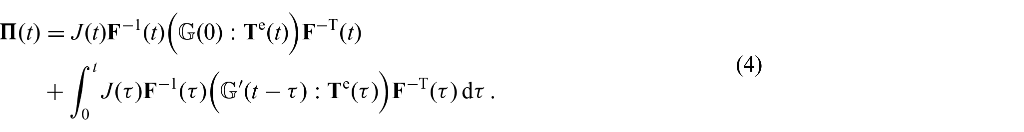
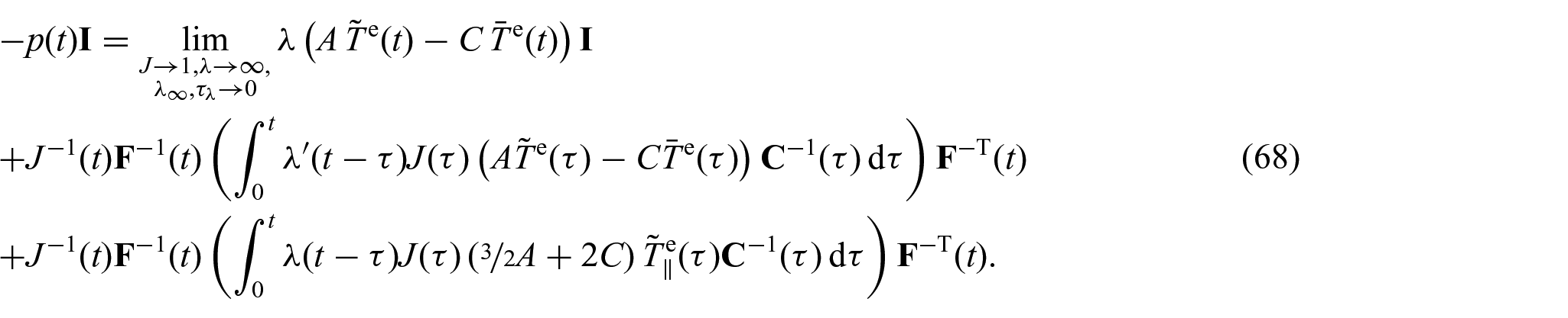
The QLV theory essentially extends the linear viscoelastic theory to the large deformation regime and allows one to account for the non-linear elastic stress–strain response of a material by writing the constitutive equation with respect to the elastic stress instead of the strain tensor. In order to satisfy objectivity, the general form of the constitutive equation is written with respect to the second Piola–Kirchhoff stress $\mathbf{\Pi }(t)$ . To obtain the MQLV model in equation (4), we start from equation (3) and we integrate by parts:

$$\begin{array}{c}\mathbf{\Pi }(t)=\sum _{n=1}^N{G}_n(0){\mathbb{K}}_n(t):(J(t){\mathbf{F}}^{-1}(t){\mathbf{T}}^{\mathrm{e}}(t){\mathbf{F}}^{-\mathrm{T}}(t))\hfill \\ \multicolumn{1}{c}{+{\int }_0^t\sum _{n=1}^N{G}_n^{\prime }(t-\tau ){\mathbb{K}}_n(\tau ):(J(\tau ){\mathbf{F}}^{-1}(\tau ){\mathbf{T}}^{\mathrm{e}}(\tau ){\mathbf{F}}^{-\mathrm{T}}(\tau ))\mathrm{d}\tau }\\ \multicolumn{1}{c}{-{\int }_0^t\sum _{n=1}^N{G}_n(t-\tau ){\mathbb{K}}_n^{\prime }(\tau ):(J(\tau ){\mathbf{F}}^{-1}(\tau ){\mathbf{T}}^{\mathrm{e}}(\tau ){\mathbf{F}}^{-\mathrm{T}}(\tau ))\mathrm{d}\tau .}\end{array}$$

(53)

The MQLV theory applies the bases ${\mathbb{K}}_n(t)$ directly to the elastic Cauchy stress ${\mathbf{T}}^{\mathrm{e}}$ , as follows:

$$\begin{array}{c}\mathbf{\Pi }(t)=\sum _{n=1}^N{G}_n(0){\mathbf{\Pi }}_n^{\mathrm{e}}(t)+{\int }_0^t\sum _{n=1}^N{G}_n^{\prime }(t-\tau ){\mathbf{\Pi }}_n^{\mathrm{e}}(\tau )\mathrm{d}\tau -{\int }_0^t\sum _{n=1}^N{G}_n(t-\tau ){\mathbf{\Omega }}_n^{\mathrm{e}}(t)\mathrm{d}\tau ,\hfill \end{array}$$

(54)

where we have defined the following terms:

$$\begin{array}{c}{\mathbf{\Pi }}_n^{\mathrm{e}}=J{\mathbf{F}}^{-1}{\mathbf{T}}_n^{\mathrm{e}}{\mathbf{F}}^{-\mathrm{T}}=J{\mathbf{F}}^{-1}({\mathbb{K}}_n:{\mathbf{T}}^{\mathrm{e}}){\mathbf{F}}^{-\mathrm{T}},\hfill \\ \multicolumn{1}{c}{{\mathbf{\Omega }}_n^{\mathrm{e}}=J{\mathbf{F}}^{-1}{\mathbf{\omega }}_n^{\mathrm{e}}{\mathbf{F}}^{-\mathrm{T}}=J{\mathbf{F}}^{-1}({\mathbb{K}}_n^{\prime }:{\mathbf{T}}^{\mathrm{e}}){\mathbf{F}}^{-\mathrm{T}}.}\end{array}$$

(55)

The term outside of the integrals gives the elastic second Piola–Kirchhoff stress, provided that the set of bases ${\mathbb{K}}_n$ is symmetrically additive and the components of $\mathbb{G}$ satisfy the condition $G_n(0)=1,\forall n\in \{1,\dots ,N\}$ . We remark that the symmetrically additive property is crucial in order for the constitutive equation to be consistent with the elastic limit. Moreover, we note that the two integrals in equation (54) arise from the fact that, in the general formulation, the bases ${\mathbb{K}}_n(t)$ depend on time $t$ .

Finally, we recall that the MQLV model is not derived mathematically from the original QLV form proposed by Fung. Indeed, although the MQLV model formally resembles the QLV model, they are two different constitutive equations. The main difference is in the bases that split the tensorial relaxation function: in the QLV model, the bases must be written with respect to the undeformed fibre vector $\mathbf{M}$ , whereas in the MQLV model, the bases must be written with respect to the deformed fibre vector ( $\mathbf{m}$ or else its normalised counterpart $\hat{\mathbf{m}}$ ) in order for the constitutive equation to be objective.

In the following sections, we will show that in the isotropic setting, the bases are time-independent (see equation (5)); therefore, the second integral in equation (54) is identically zero. However, in the TI setting, the bases do depend on time and the deformation in general. We will illustrate this property by considering specific deformations.

4.1. Isotropy

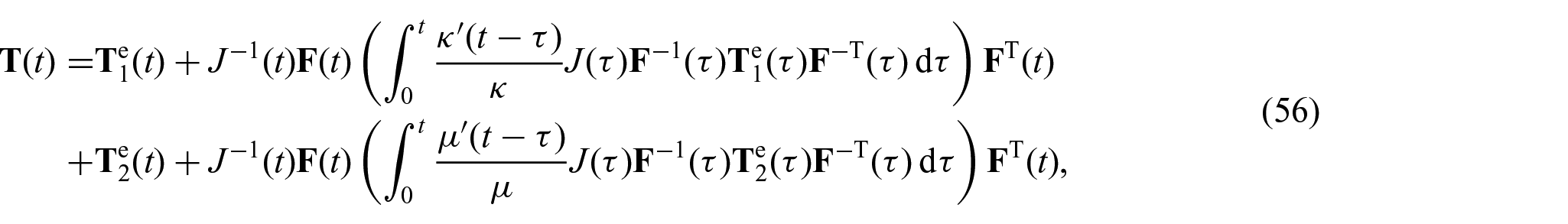
The isotropic case was extensively studied in De Pascalis et al. [7]. For completeness, we recall here the compressible and incompressible forms. Using the Piola transformation [19], the Cauchy stress for a compressible material can be written as:

$$\begin{array}{c}\mathbf{T}(t)={\mathbf{T}}_1^{\mathrm{e}}(t)+J^{-1}(t)\mathbf{F}(t)({\int }_0^t\frac{{\kappa }^{\prime }(t-\tau )}{\kappa }J(\tau ){\mathbf{F}}^{-1}(\tau ){\mathbf{T}}_1^{\mathrm{e}}(\tau ){\mathbf{F}}^{-\mathrm{T}}(\tau )\mathrm{d}\tau ){\mathbf{F}}^{\mathrm{T}}(t)\hfill \\ \multicolumn{1}{c}{+{\mathbf{T}}_2^{\mathrm{e}}(t)+J^{-1}(t)\mathbf{F}(t)({\int }_0^t\frac{{\mu }^{\prime }(t-\tau )}{\mu }J(\tau ){\mathbf{F}}^{-1}(\tau ){\mathbf{T}}_2^{\mathrm{e}}(\tau ){\mathbf{F}}^{-\mathrm{T}}(\tau )\mathrm{d}\tau ){\mathbf{F}}^{\mathrm{T}}(t),}\end{array}$$

(56)

where:

$${\mathbf{T}}_1^{\mathrm{e}}=\frac{1}{3}\mathrm{tr}[{\mathbf{T}}^{\mathrm{e}}]\mathbf{I}\mathrm{and}{\mathbf{T}}_2^{\mathrm{e}}={\mathbf{T}}^{\mathrm{e}}-\frac{1}{3}\mathrm{tr}[{\mathbf{T}}^{\mathrm{e}}]\mathbf{I}=\mathrm{dev}[{\mathbf{T}}^{\mathrm{e}}],$$

(57)

and we have replaced ${\mathbb{K}}_n$ with the symmetrically additive bases in equation (34) and the components $G_1$ and $G_2$ with the connections in equation (18).

We assume a Prony series form for the relaxation functions $\kappa (t)$ and $\mu (t)$ such that:

$$\kappa (t)={\kappa }_{\infty }+(\kappa -{\kappa }_{\infty })e^{-\mathrm{t}/{\tau }_{\kappa }}\mathrm{and}\mu (t)={\mu }_{\infty }+(\mu -{\mu }_{\infty })e^{-\mathrm{t}/{\tau }_{\mu }}.$$

(58)

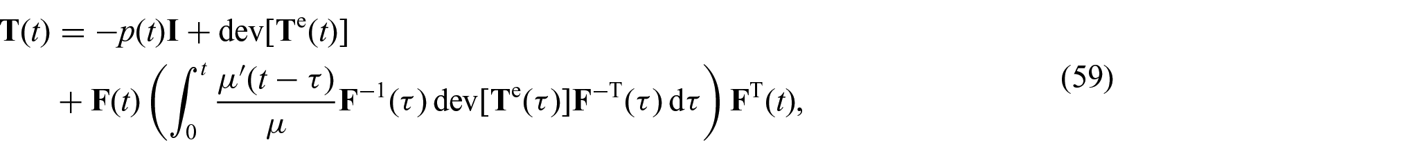
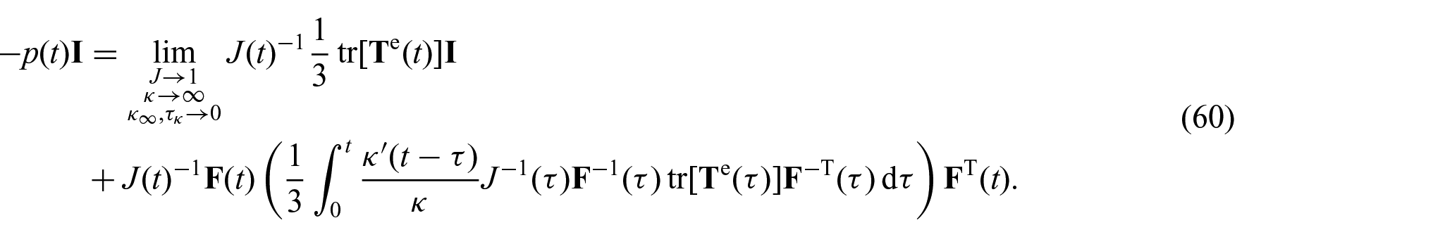
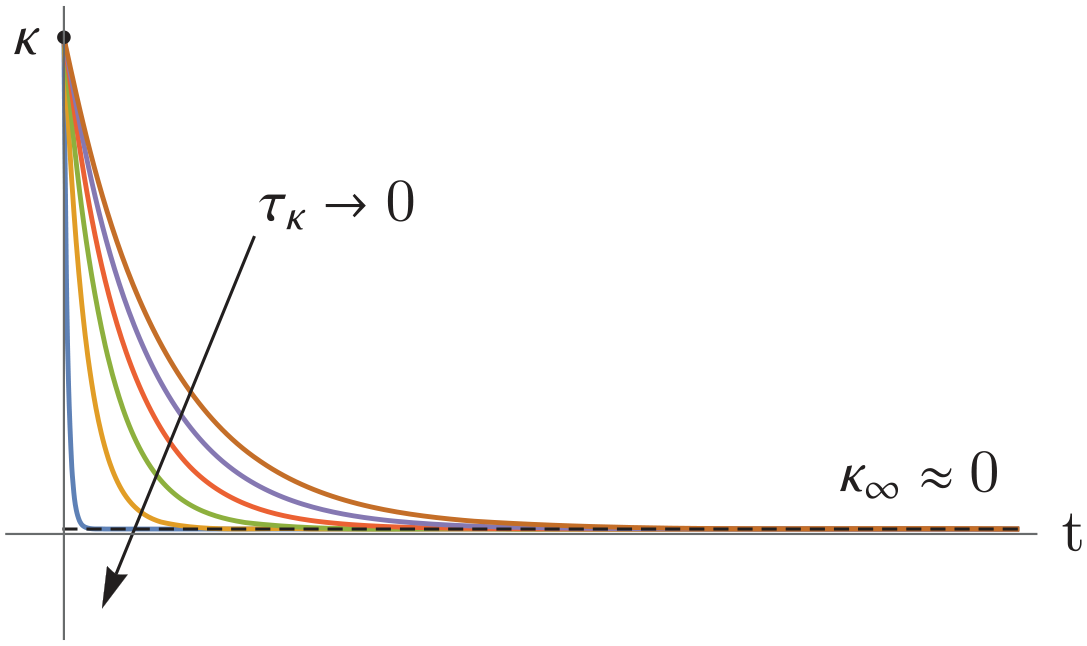
In the incompressible limit, we assume that the elastic bulk modulus is much greater than the elastic shear modulus so that $\kappa \to \infty$ . Moreover, we take the characteristic time ${\tau }_{\kappa }$ and the long-term bulk modulus ${\kappa }_{\infty }$ to be close to zero in the incompressible limit. These assumptions correspond to the incompressible contributions being instantaneous (elastic) only. In Figure 1, we show the behaviour of the relaxation function associated with the bulk modulus in the incompressible limit. Finally, for isochoric deformations, we have $J(t)=1,\forall t$ . Under this assumptions, we can rewrite equation (56) as follows:

$$\begin{array}{c}\mathbf{T}(t)=-p(t)\mathbf{I}+\mathrm{dev}[{\mathbf{T}}^{\mathrm{e}}(t)]\hfill \\ \multicolumn{1}{c}{+\mathbf{F}(t)({\int }_0^t\frac{{\mu }^{\prime }(t-\tau )}{\mu }{\mathbf{F}}^{-1}(\tau )\mathrm{dev}[{\mathbf{T}}^{\mathrm{e}}(\tau )]{\mathbf{F}}^{-\mathrm{T}}(\tau )\mathrm{d}\tau ){\mathbf{F}}^{\mathrm{T}}(t),}\end{array}$$

(59)

where the Lagrange multiplier $p(t)$ is given by:

$$\begin{array}{c}-p(t)\mathbf{I}=\underset{\genfrac{}{}{0ex}{}{J\to 1}{\genfrac{}{}{0ex}{}{\kappa \to \infty }{{\kappa }_{\infty },{\tau }_{\kappa }\to 0}}}{lim}J{(t)}^{-1}\frac{1}{3}\mathrm{tr}[{\mathbf{T}}^{\mathrm{e}}(t)]\mathbf{I}\hfill \\ \multicolumn{1}{c}{+J{(t)}^{-1}\mathbf{F}(t)(\frac{1}{3}{\int }_0^t\frac{{\kappa }^{\prime }(t-\tau )}{\kappa }{J}^{-1}(\tau ){\mathbf{F}}^{-1}(\tau )\mathrm{tr}[T^{\mathrm{e}}(\tau )]{\mathbf{F}}^{-\mathrm{T}}(\tau )\mathrm{d}\tau ){\mathbf{F}}^{\mathrm{T}}(t).}\end{array}$$

(60)

Figure 1.

Behaviour of the relaxation function $\kappa (t)$ as the characteristic time ${\tau }_{\kappa }\to 0$ . The long-term equilibrium bulk modulus is set to ${\kappa }_{\infty }=0.01$ and the curves are plotted for ${\tau }_{\kappa }=\{0.52,0.42,0.32,0.22,0.12,0.02\}$ .

4.2. Transverse isotropy

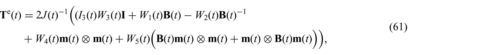
We call $\mathbf{M}$ the unit vector that identifies the preferred direction of the TI material in the initial undeformed configuration and $\mathbf{m}(t)=F(t)\mathbf{M}$ the equivalent deformed fibre vector. For a compressible TI material, the constitutive equation for the elastic Cauchy stress is given by:

$$\begin{array}{c}{\mathbf{T}}^{\mathrm{e}}(t)=2J{(t)}^{-1}((I_3(t)W_3(t)\mathbf{I}+W_1(t)\mathbf{B}(t)-W_2(t)\mathbf{B}{(t)}^{-1}\hfill \\ \multicolumn{1}{c}{+W_4(t)\mathbf{m}(t)\otimes \mathbf{m}(t)+W_5(t)(\mathbf{B}(t)\mathbf{m}(t)\otimes \mathbf{m}(t)+\mathbf{m}(t)\otimes \mathbf{B}(t)\mathbf{m}(t))),}\end{array}$$

(61)

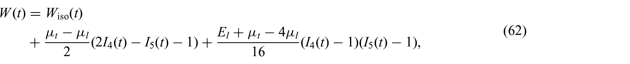
where $J(t)=\det \mathbf{F}(t)$ , $W_i(t)=\partial W(t)/\partial I_i(t)$ $(i=\{1,\dots ,5\})$ , and $I_i$ are the invariants of $\mathbf{B}(t)$ (see Ogden [19] for the full details). For the strain energy function $W(t)$ , we choose the following form:

$$\begin{array}{c}W(t)=W_{\mathrm{iso}}(t)\hfill \\ \multicolumn{1}{c}{+\frac{{\mu }_t-{\mu }_l}{2}(2I_4(t)-I_5(t)-1)+\frac{E_l+{\mu }_t-4{\mu }_l}{16}(I_4(t)-1)(I_5(t)-1),}\end{array}$$

(62)

where

$$W_{\mathrm{iso}}(t)=\frac{{\mu }_t}{2}({\alpha }_{\mathrm{MR}}(I_1(t)-3)+(1-{\alpha }_{\mathrm{MR}})(I_2(t)-3)),\mathrm{with}{\alpha }_{\mathrm{MR}}\in [0,1],$$

(63)

which is consistent with the linear theory in the small strain limit [20].

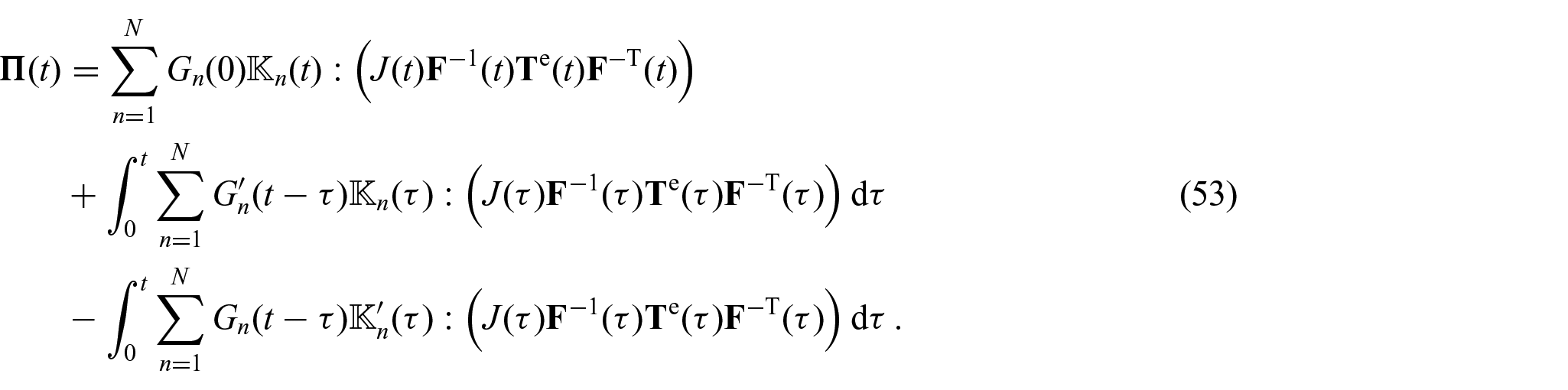
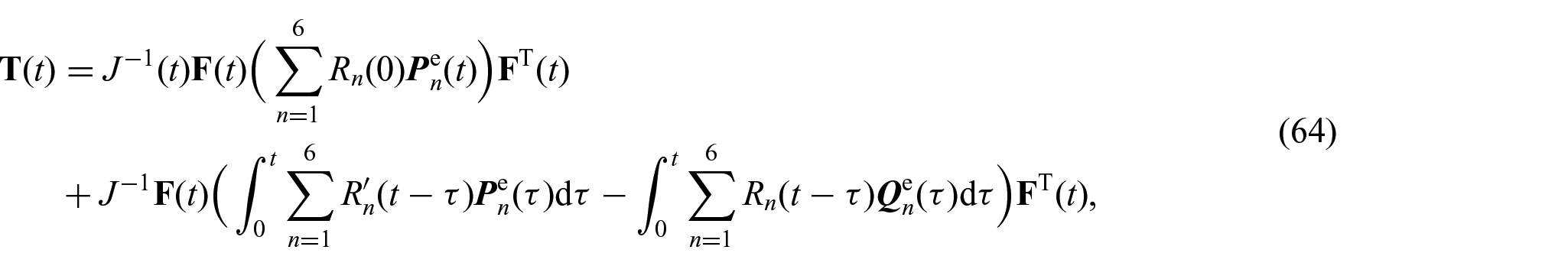
Now, to write the MQLV model, we choose the symmetrically additive Hill bases; therefore, the constitutive equation (54) for compressible TI materials can be written as follows:

$$\begin{array}{c}\mathbf{T}(t)=J^{-1}(t)\mathbf{F}(t)(\sum _{n=1}^6{R}_n(0){\mathit{P}}_n^{\mathrm{e}}(t)){\mathbf{F}}^{\mathrm{T}}(t)\hfill \\ \multicolumn{1}{c}{+J^{-1}\mathbf{F}(t)({\int }_0^t\sum _{n=1}^6{R}_n^{\prime }(t-\tau ){\mathit{P}}_n^{\mathrm{e}}(\tau )\mathrm{d}\tau -{\int }_0^t\sum _{n=1}^6{R}_n(t-\tau ){\mathit{Q}}_n^{\mathrm{e}}(\tau )\mathrm{d}\tau ){\mathbf{F}}^{\mathrm{T}}(t),}\end{array}$$

(64)

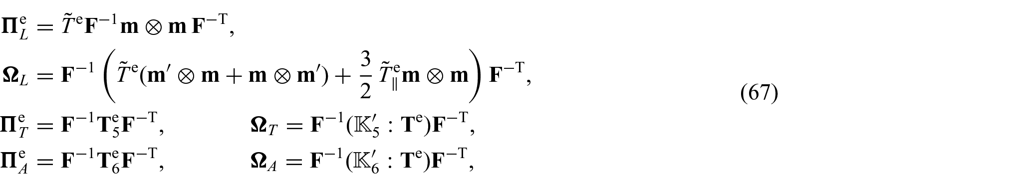
where we have used the connection in equation (52) to replace the components $G_n$ , with the relaxation functions $R_n$ , $n=\{1,\dots ,6\}$ . The terms ${\mathit{P}}_n^{\mathrm{e}}$ and ${\mathit{Q}}_n^{\mathrm{e}}$ are given in Appendix 1.

In the incompressible limit, we assume that the relaxation function $\lambda (t)$ behaves as the function $\kappa (t)$ in Figure 1, with $\lambda \to \infty$ and ${\tau }_{\lambda },{\lambda }_{\infty }\to 0$ . Therefore:

$$\underset{\lambda \to \infty }{lim}A=\underset{\lambda \to \infty }{lim}C=\underset{\lambda \to \infty }{lim}D=0\mathrm{and}\underset{\lambda \to \infty }{lim}B=\frac{1}{\beta +4{\mu }_l-{\mu }_t}=\frac{1}{E_l},$$

(65)

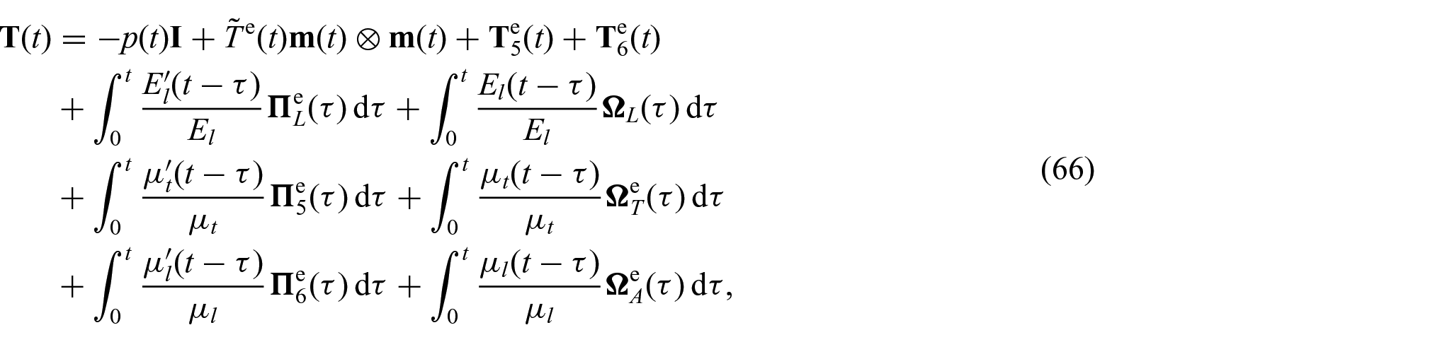
where $E_l$ is the elastic longitudinal Young modulus. Moreover, in the incompressible limit, $\alpha \to {\mu }_t$ ; therefore, we take $\alpha (t)\to {\mu }_t(t),\forall t$ . Under these assumptions, the constitutive equation (64) can be rewritten as follows:

$$\begin{array}{c}\mathbf{T}(t)=-p(t)\mathbf{I}+{\tilde{T}}^{\mathrm{e}}(t)\mathbf{m}(t)\otimes \mathbf{m}(t)+{\mathbf{T}}_5^{\mathrm{e}}(t)+{\mathbf{T}}_6^{\mathrm{e}}(t)\hfill \\ \multicolumn{1}{c}{+{\int }_0^t\frac{E_l^{\prime }(t-\tau )}{E_l}{\mathbf{\Pi }}_L^{\mathrm{e}}(\tau )\mathrm{d}\tau +{\int }_0^t\frac{E_l(t-\tau )}{E_l}{\mathbf{\Omega }}_L(\tau )\mathrm{d}\tau }\\ \multicolumn{1}{c}{+{\int }_0^t\frac{{\mu }_t^{\prime }(t-\tau )}{{\mu }_t}{\mathbf{\Pi }}_5^{\mathrm{e}}(\tau )\mathrm{d}\tau +{\int }_0^t\frac{{\mu }_t(t-\tau )}{{\mu }_t}{\mathbf{\Omega }}_T^{\mathrm{e}}(\tau )\mathrm{d}\tau }\\ \multicolumn{1}{c}{+{\int }_0^t\frac{{\mu }_l^{\prime }(t-\tau )}{{\mu }_l}{\mathbf{\Pi }}_6^{\mathrm{e}}(\tau )\mathrm{d}\tau +{\int }_0^t\frac{{\mu }_l(t-\tau )}{{\mu }_l}{\mathbf{\Omega }}_A^{\mathrm{e}}(\tau )\mathrm{d}\tau ,}\end{array}$$

(66)

where:

$$\begin{array}{c}{\mathbf{\Pi }}_L^{\mathrm{e}}={\tilde{T}}^{\mathrm{e}}{\mathbf{F}}^{-1}\mathbf{m}\otimes \mathbf{m}{\mathbf{F}}^{-\mathrm{T}},\hfill \\ \multicolumn{1}{c}{{\mathbf{\Omega }}_L={\mathbf{F}}^{-1}({\tilde{T}}^{\mathrm{e}}({\mathbf{m}}^{\prime }\otimes \mathbf{m}+\mathbf{m}\otimes {\mathbf{m}}^{\prime })+\frac{3}{2}{\tilde{T}}_{\parallel }^{\mathrm{e}}\mathbf{m}\otimes \mathbf{m}){\mathbf{F}}^{-\mathrm{T}},}\\ \multicolumn{1}{c}{{\mathbf{\Pi }}_T^{\mathrm{e}}={\mathbf{F}}^{-1}{\mathbf{T}}_5^{\mathrm{e}}{\mathbf{F}}^{-\mathrm{T}},{\mathbf{\Omega }}_T={\mathbf{F}}^{-1}({\mathbb{K}}_5^{\prime }:{\mathbf{T}}^{\mathrm{e}}){\mathbf{F}}^{-\mathrm{T}},}\\ \multicolumn{1}{c}{{\mathbf{\Pi }}_A^{\mathrm{e}}={\mathbf{F}}^{-1}{\mathbf{T}}_6^{\mathrm{e}}{\mathbf{F}}^{-\mathrm{T}},{\mathbf{\Omega }}_A={\mathbf{F}}^{-1}({\mathbb{K}}_6^{\prime }:{\mathbf{T}}^{\mathrm{e}}){\mathbf{F}}^{-\mathrm{T}},}\end{array}$$

(67)

and $E_l(t)=\beta (t)-{\mu }_t(t)+4{\mu }_l(t)$ . The Lagrange multiplier $p(t)$ is given by:

$$\begin{array}{c}-p(t)\mathbf{I}=\underset{\genfrac{}{}{0ex}{}{J\to 1,\lambda \to \infty ,}{{\lambda }_{\infty },{\tau }_{\lambda }\to 0}}{lim}\lambda (A{\tilde{T}}^{\mathrm{e}}(t)-C{\overline{T}}^{\mathrm{e}}(t))\mathbf{I}\hfill \\ \multicolumn{1}{c}{+J^{-1}(t){\mathbf{F}}^{-1}(t)({\int }_0^t{\lambda }^{\prime }(t-\tau )J(\tau )(A{\tilde{T}}^{\mathrm{e}}(\tau )-C{\overline{T}}^{\mathrm{e}}(\tau )){\mathbf{C}}^{-1}(\tau )\mathrm{d}\tau ){\mathbf{F}}^{-\mathrm{T}}(t)}\\ \multicolumn{1}{c}{+J^{-1}(t){\mathbf{F}}^{-1}(t)({\int }_0^t\lambda (t-\tau )J(\tau )(32A+2C){\tilde{T}}_{\parallel }^{\mathrm{e}}(\tau ){\mathbf{C}}^{-1}(\tau )\mathrm{d}\tau ){\mathbf{F}}^{-\mathrm{T}}(t).}\end{array}$$

(68)

In the next section, we illustrate the key features of the MQLV model for TI materials.

5. Strain-dependent relaxation

A key feature of the MQLV model for TI materials is that the constitutive equation is able to capture strain-dependent relaxation. This non-linear property is a direct consequence of the bases being dependent on the deformed fibre vector $\mathbf{m}(t)$ . The vector $\mathbf{m}(t)$ depends on the deformation through the deformation gradient $\mathbf{F}(t)$ . This naturally introduces a dependence on the deformation in the relaxation tensor $\mathbb{G}(t)$ . Therefore, the model naturally captures the non-linear phenomenon of strain-dependent relaxation, which is commonly observed in soft materials such as soft tissues and gels, whereby the relaxation curve is affected by the level of strain reached during a step-strain test [3, 21–23].

We note that the bases used in the constitutive equation (66) are written with respect to the vector $\mathbf{m}(t)$ . However, an alternative formulation (which was proposed in Balbi et al. [8]) allows us to write the bases with respect to the unit deformed vector:

$$\hat{\mathbf{m}}(t)=\frac{\mathbf{m}(t)}{\parallel \mathbf{m}(t)\parallel }=\frac{\mathbf{F}(t)\mathbf{M}}{\sqrt{\mathbf{F}(t)\mathbf{M}·\mathbf{F}(t)\mathbf{M}}}.$$

(69)

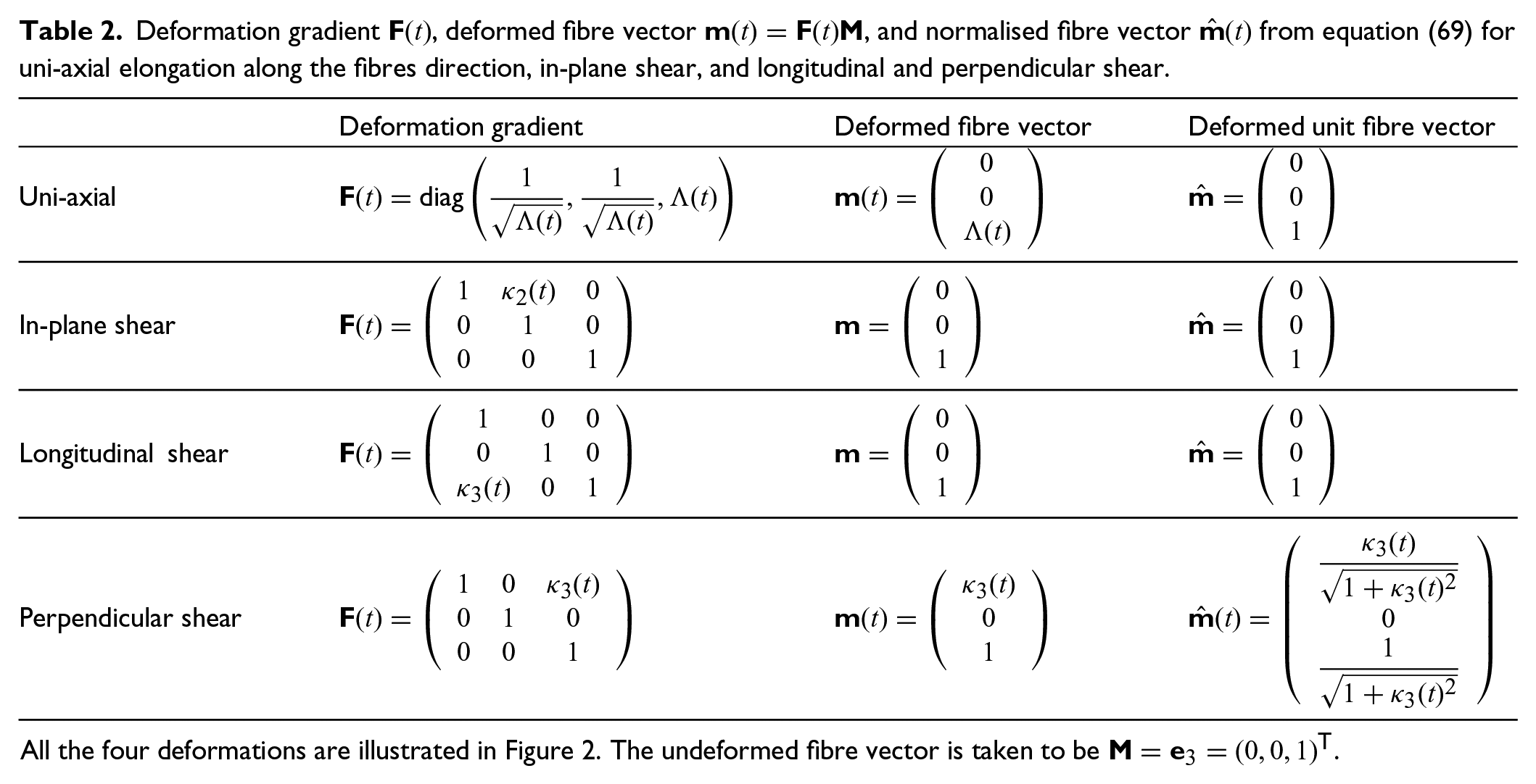
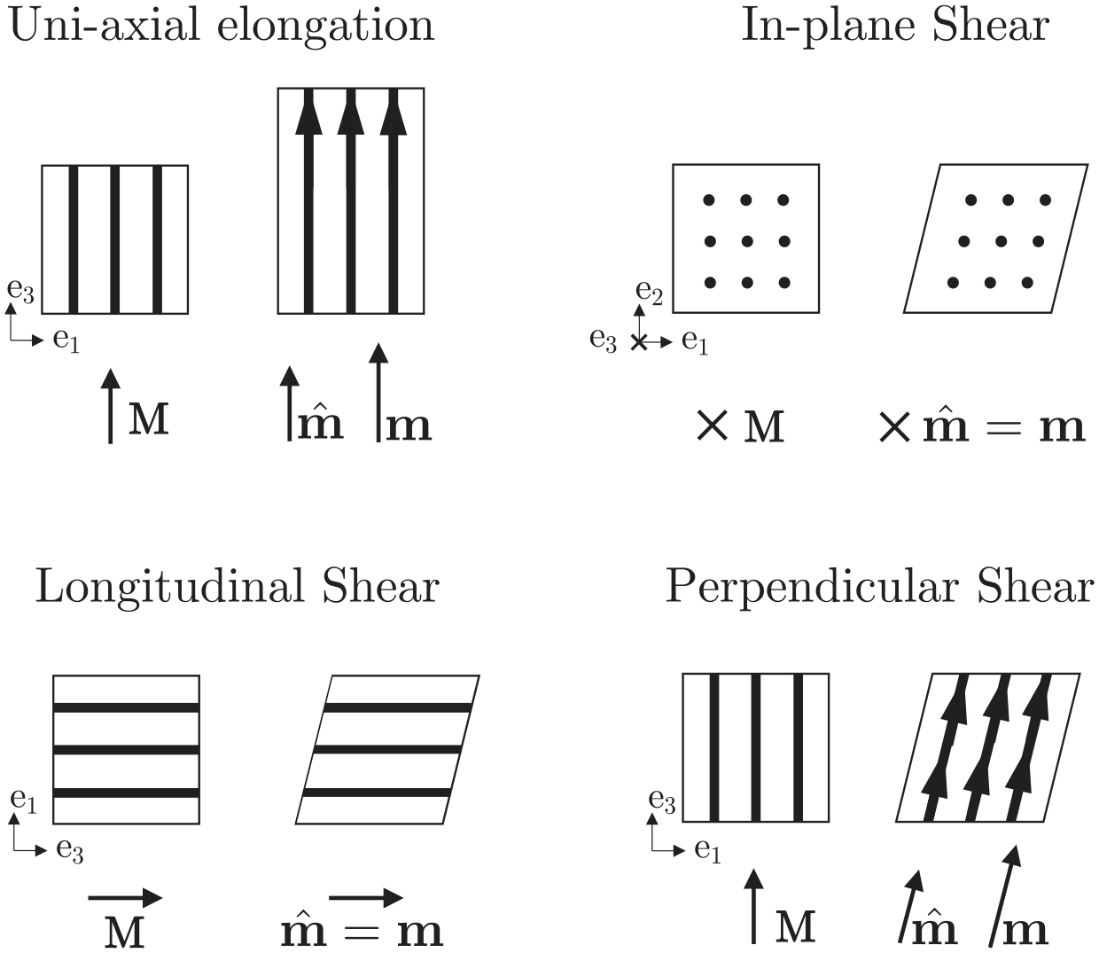
In Table 2, we consider the case of a fibre-reinforced TI material and we compare the vectors $\hat{\mathbf{m}}$ and $\mathbf{m}$ for the most common deformation modes used in mechanical testing. These are uni-axial extension, in-plane shear (i.e., shear in the isotropic plane), longitudinal and perpendicular shear (i.e., shear along the fibre and perpendicular to the fibre direction, respectively). The fibres in the undeformed material are assumed to be aligned along the vector $\mathbf{M}=(0,0,1{)}^{\mathrm{T}}$ . The two versions of the MQLV theory are equivalent for deformation modes where $\hat{\mathbf{m}}=\mathbf{m}$ , i.e., in-plane and longitudinal shear. For these deformation modes, the fibres do not deform; therefore, $\hat{\mathbf{m}}=\mathbf{m}=\mathbf{M}$ , as shown in Figure 2. However, they differ under uni-axial extension and perpendicular shear, which we consider below.

Table 2.

Deformation gradient $\mathbf{F}(t)$ , deformed fibre vector $\mathbf{m}(t)=\mathbf{F}(t)\mathbf{M}$ , and normalised fibre vector $\hat{\mathbf{m}}(t)$ from equation (69) for uni-axial elongation along the fibres direction, in-plane shear, and longitudinal and perpendicular shear.

	Deformation gradient	Deformed fibre vector	Deformed unit fibre vector
Uni-axial	$\mathbf{F}(t)=\mathrm{diag}(\frac{1}{\sqrt{\mathrm{\Lambda }(t)}},\frac{1}{\sqrt{\mathrm{\Lambda }(t)}},\mathrm{\Lambda }(t))$	$\mathbf{m}(t)=\left(\begin{array}{c}0\hfill \\ \multicolumn{1}{c}{0}\\ \multicolumn{1}{c}{\mathrm{\Lambda }(t)}\end{array}\right)$	$\hat{\mathbf{m}}=\left(\begin{array}{c}0\hfill \\ \multicolumn{1}{c}{0}\\ \multicolumn{1}{c}{1}\end{array}\right)$
In-plane shear	$\mathbf{F}(t)=\left(\begin{array}{ccc}1\hfill & {\kappa }_2(t)\hfill & 0\hfill \\ \multicolumn{1}{c}{0}& 1\hfill & 0\hfill \\ \multicolumn{1}{c}{0}& 0\hfill & 1\hfill \end{array}\right)$	$\mathbf{m}=\left(\begin{array}{c}0\hfill \\ \multicolumn{1}{c}{0}\\ \multicolumn{1}{c}{1}\end{array}\right)$	$\hat{\mathbf{m}}=\left(\begin{array}{c}0\hfill \\ \multicolumn{1}{c}{0}\\ \multicolumn{1}{c}{1}\end{array}\right)$
Longitudinal shear	$\mathbf{F}(t)=\left(\begin{array}{ccc}1\hfill & 0\hfill & 0\hfill \\ \multicolumn{1}{c}{0}& 1\hfill & 0\hfill \\ \multicolumn{1}{c}{{\kappa }_3(t)}& 0\hfill & 1\hfill \end{array}\right)$	$\mathbf{m}=\left(\begin{array}{c}0\hfill \\ \multicolumn{1}{c}{0}\\ \multicolumn{1}{c}{1}\end{array}\right)$	$\hat{\mathbf{m}}=\left(\begin{array}{c}0\hfill \\ \multicolumn{1}{c}{0}\\ \multicolumn{1}{c}{1}\end{array}\right)$
Perpendicular shear	$\mathbf{F}(t)=\left(\begin{array}{ccc}1\hfill & 0\hfill & {\kappa }_3(t)\hfill \\ \multicolumn{1}{c}{0}& 1\hfill & 0\hfill \\ \multicolumn{1}{c}{0}& 0\hfill & 1\hfill \end{array}\right)$	$\mathbf{m}(t)=\left(\begin{array}{c}{\kappa }_3(t)\hfill \\ \multicolumn{1}{c}{0}\\ \multicolumn{1}{c}{1}\end{array}\right)$	$\hat{\mathbf{m}}(t)=\left(\begin{array}{c}\frac{{\kappa }_3(t)}{\sqrt{1+{\kappa }_3{(t)}^2}}\hfill \\ \multicolumn{1}{c}{0}\\ \multicolumn{1}{c}{\frac{1}{\sqrt{1+{\kappa }_3{(t)}^2}}}\end{array}\right)$

All the four deformations are illustrated in Figure 2. The undeformed fibre vector is taken to be $\mathbf{M}={\mathbf{e}}_3=(0,0,1{)}^{\top }$ .

Figure 2.

Deformation modes for a fibre-reinforced TI material: in uni-axial elongation, the fibres stretch ( $\hat{\mathbf{m}}=\mathbf{M}$ and $\mathbf{m}(t)=(0,0,\mathrm{\Lambda }(t){)}^{\top }$ ); under in-plane and longitudinal shear, the fibres do not deform $(\hat{\mathbf{m}}=\mathbf{m}=\mathbf{M})$ ; in perpendicular shear, the fibres stretch and rotate $(\hat{\mathbf{m}}(t)\ne \mathbf{m}(t)\ne \mathbf{M})$ .

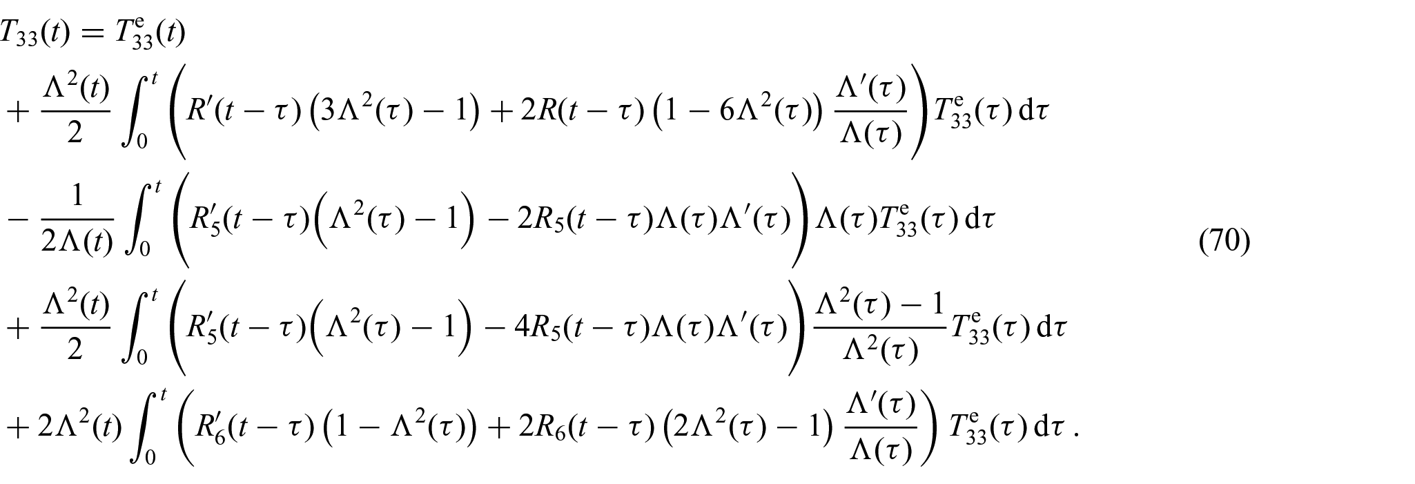
Let us compare the predictions of the two models under uni-axial elongation. In this case, the fibres are stretched while the material is deformed; therefore, $\hat{\mathbf{m}}\ne \mathbf{m}$ (see Table 2). By assuming the lateral surfaces to be free of traction, the only non-zero component of the Cauchy stress is $T_{33}(t)$ , which can be calculated from equation (66) using the corresponding deformation gradient in Table 2 (see Appendix 1 for the detailed derivation):

$$\begin{array}{c}{T}_{33}(t)=T_{33}^{\mathrm{e}}(t)\hfill \\ \multicolumn{1}{c}{+\frac{{\mathrm{\Lambda }}^2(t)}{2}{\int }_0^t(R^{\prime }(t-\tau )(3{\mathrm{\Lambda }}^2(\tau )-1)+2R(t-\tau )(1-6{\mathrm{\Lambda }}^2(\tau ))\frac{{\mathrm{\Lambda }}^{\prime }(\tau )}{\mathrm{\Lambda }(\tau )})T_{33}^{\mathrm{e}}(\tau )\mathrm{d}\tau }\\ \multicolumn{1}{c}{-\frac{1}{2\mathrm{\Lambda }(t)}{\int }_0^t(R_5^{\prime }(t-\tau )({\mathrm{\Lambda }}^2(\tau )-1)-2R_5(t-\tau )\mathrm{\Lambda }(\tau ){\mathrm{\Lambda }}^{\prime }(\tau ))\mathrm{\Lambda }(\tau )T_{33}^{\mathrm{e}}(\tau )\mathrm{d}\tau }\\ \multicolumn{1}{c}{+\frac{{\mathrm{\Lambda }}^2(t)}{2}{\int }_0^t(R_5^{\prime }(t-\tau )({\mathrm{\Lambda }}^2(\tau )-1)-4R_5(t-\tau )\mathrm{\Lambda }(\tau ){\mathrm{\Lambda }}^{\prime }(\tau ))\frac{{\mathrm{\Lambda }}^2(\tau )-1}{{\mathrm{\Lambda }}^2(\tau )}{T}_{33}^{\mathrm{e}}(\tau )\mathrm{d}\tau }\\ \multicolumn{1}{c}{+2{\mathrm{\Lambda }}^2(t){\int }_0^t(R_6^{\prime }(t-\tau )(1-{\mathrm{\Lambda }}^2(\tau ))+2R_6(t-\tau )(2{\mathrm{\Lambda }}^2(\tau )-1)\frac{{\mathrm{\Lambda }}^{\prime }(\tau )}{\mathrm{\Lambda }(\tau )})T_{33}^{\mathrm{e}}(\tau )\mathrm{d}\tau .}\end{array}$$

(70)

We recall below the expression for the stress $T_{33}$ derived in Balbi et al. [8] for the MQLV model under uni-axial extension, where the bases are written with respect to the normalised vector $\hat{\mathbf{m}}$ :

$$T_{33}(t)=T_{33}^{\mathrm{e}}(t)+\mathrm{\Lambda }(t{)}^2{\int }_0^t\frac{{\mathcal{R}}^{\prime }(t-\tau )}{E_l}\frac{T_{33}(\tau )}{\mathrm{\Lambda }(\tau )}\mathrm{d}\tau .$$

(71)

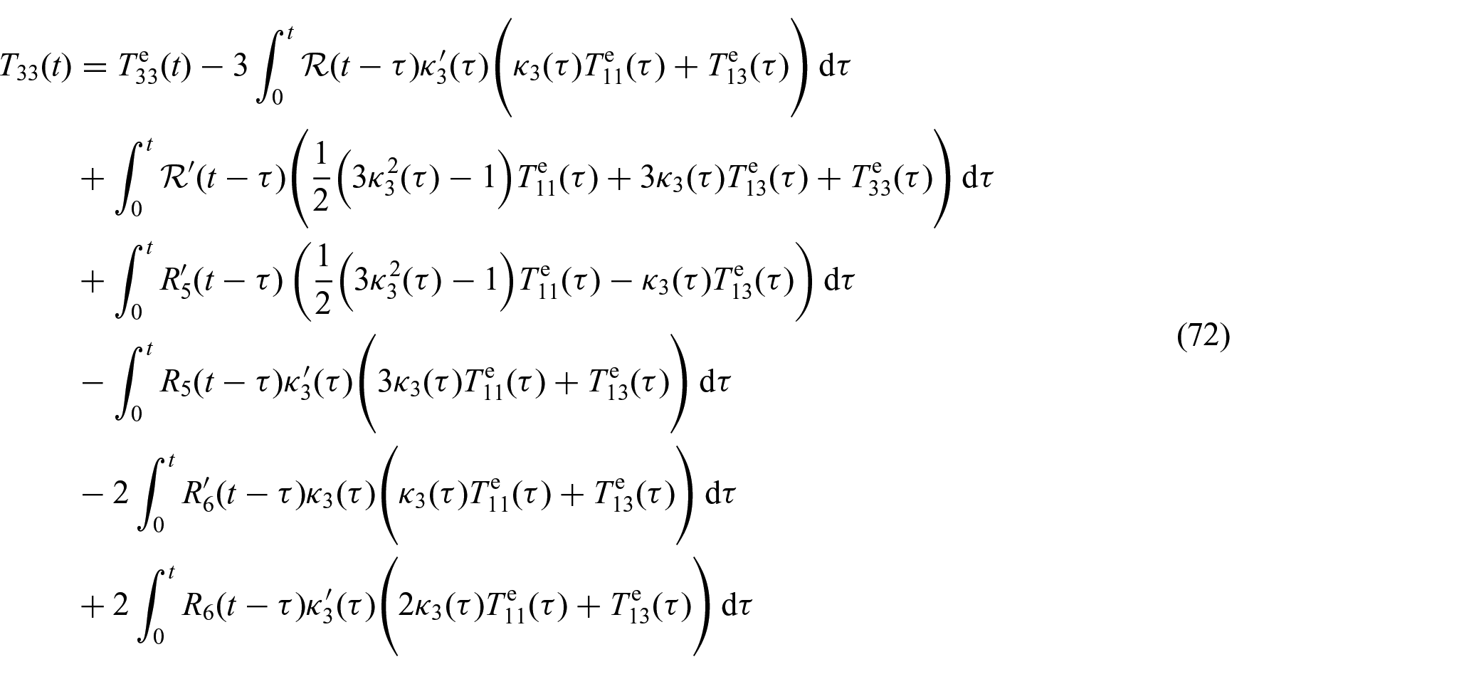
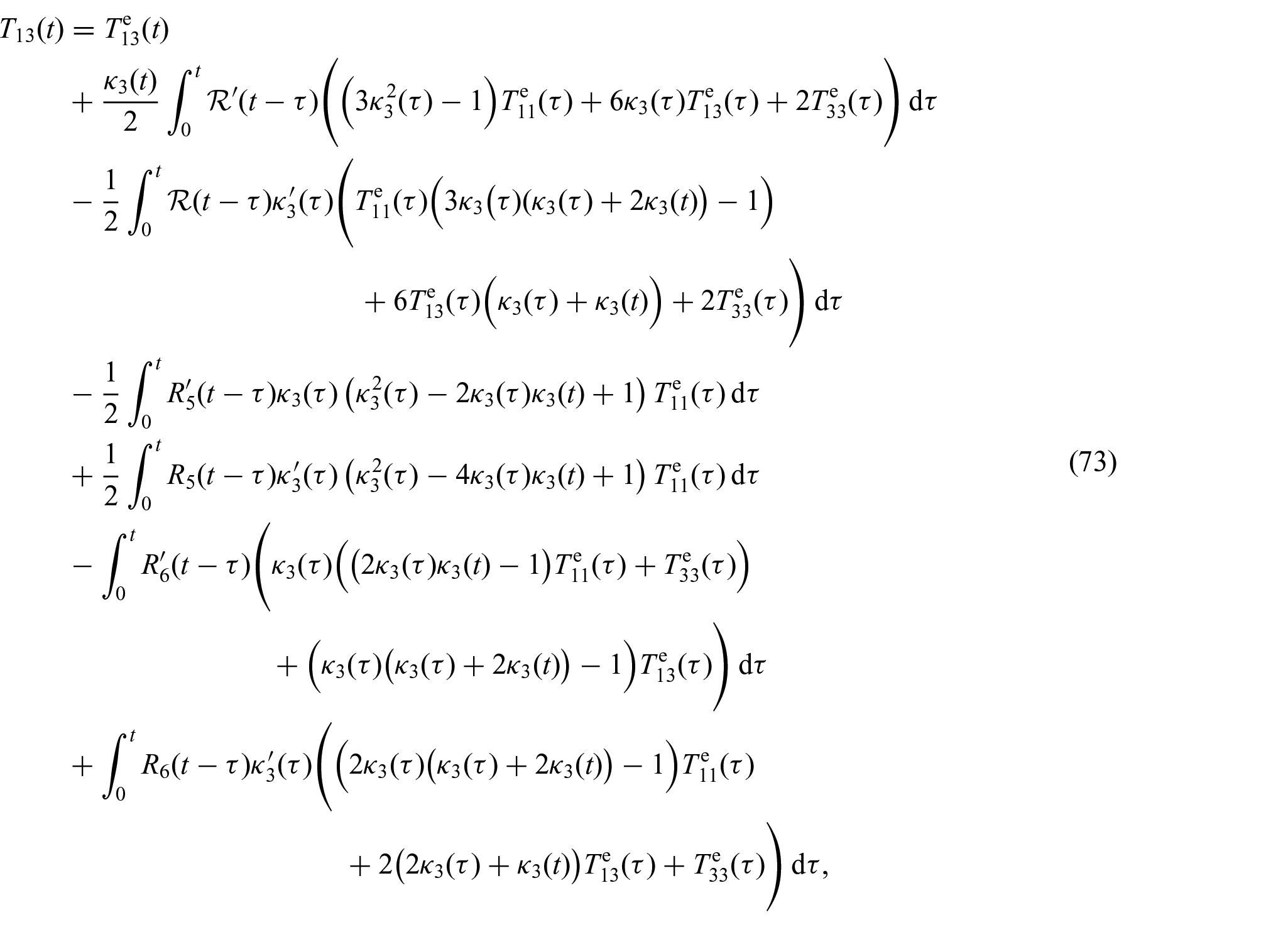
In Figure 3, we plot the relaxation curves for uni-axial extension at different levels of stretch calculated using the MQLV model via equations (70) (left) and (71) (right), where the bases are written with respect to the vectors $\mathbf{m}(t)$ and $\hat{\mathbf{m}}(t)$ , respectively. Figure 3 shows that only the model written with respect to the deformed vector $\mathbf{m}(t)$ predicts strain-dependent relaxation. This phenomenon follows from the fact that the fibre vector $\mathbf{m}(t)$ accounts for the stretching of the fibres during the deformation. The more the fibres are stretched, the more the material relaxes after the initial deformation. However, the vector $\hat{\mathbf{m}}$ only accounts for changes in the fibres’ orientation (not for changes in the magnitude of the stretching). In the small deformation limit (see the curves for $\mathrm{\Lambda }=0.05$ in Figure 3), the two versions of the MQLV model predict the same results, as expected. Indeed, $\widehat{\mathbf{m}}\approx \mathbf{m}\approx \mathbf{M}$ . The other deformation that can accommodate non-linear features is perpendicular shear. Under this deformation, by assuming the lateral sides of the rectangular block are free of traction, the only non-zero stress components are the two normal stresses, i.e., $T_{11}(t)$ and $T_{33}(t)$ , and the shear stress $T_{13}(t)$ . In particular, we look at the expressions for the normal stress $T_{33}(t)$ and the shear stress $T_{13}(t)$ . These are given by:

$$\begin{array}{c}{T}_{33}(t)=T_{33}^{\mathrm{e}}(t)-3{\int }_0^t\mathcal{R}(t-\tau ){\kappa }_3^{\prime }(\tau )({\kappa }_3(\tau )T_{11}^{\mathrm{e}}(\tau )+T_{13}^{\mathrm{e}}(\tau ))\mathrm{d}\tau \hfill \\ \multicolumn{1}{c}{+{\int }_0^t{\mathcal{R}}^{\prime }(t-\tau )(\frac{1}{2}(3{\kappa }_3^2(\tau )-1)T_{11}^{\mathrm{e}}(\tau )+3{\kappa }_3(\tau )T_{13}^{\mathrm{e}}(\tau )+T_{33}^{\mathrm{e}}(\tau ))\mathrm{d}\tau }\\ \multicolumn{1}{c}{+{\int }_0^t{R}_5^{\prime }(t-\tau )(\frac{1}{2}(3{\kappa }_3^2(\tau )-1)T_{11}^{\mathrm{e}}(\tau )-{\kappa }_3(\tau )T_{13}^{\mathrm{e}}(\tau ))\mathrm{d}\tau }\\ \multicolumn{1}{c}{-{\int }_0^t{R}_5^{\prime }(t-\tau ){\kappa }_3^{\prime }(\tau )(3{\kappa }_3(\tau )T_{11}^{\mathrm{e}}(\tau )+T_{13}^{\mathrm{e}}(\tau ))\mathrm{d}\tau }\\ \multicolumn{1}{c}{-2{\int }_0^t{R}_6^{\prime }(t-\tau ){\kappa }_3(\tau )({\kappa }_3(\tau )T_{11}^{\mathrm{e}}(\tau )+T_{13}^{\mathrm{e}}(\tau ))\mathrm{d}\tau }\\ \multicolumn{1}{c}{+2{\int }_0^t{R}_6(t-\tau ){\kappa }_3^{\prime }(\tau )(2{\kappa }_3(\tau )T_{11}^{\mathrm{e}}(\tau )+T_{13}^{\mathrm{e}}(\tau ))\mathrm{d}\tau }\end{array}$$

(72)

and

$$\begin{array}{c}{T}_{13}(t)=T_{13}^{\mathrm{e}}(t)\hfill \\ \multicolumn{1}{c}{+\frac{{\kappa }_3(t)}{2}{\int }_0^t{\mathcal{R}}^{\prime }(t-\tau )((3{\kappa }_3^2(\tau )-1)T_{11}^{\mathrm{e}}(\tau )+6{\kappa }_3(\tau )T_{13}^{\mathrm{e}}(\tau )+2T_{33}^{\mathrm{e}}(\tau ))\mathrm{d}\tau }\\ \multicolumn{1}{c}{-\frac{1}{2}{\int }_0^t\mathcal{R}(t-\tau ){\kappa }_3^{\prime }(\tau )(T_{11}^{\mathrm{e}}(\tau )(3{\kappa }_3(\tau )({\kappa }_3(\tau )+2{\kappa }_3(t))-1)}\\ \multicolumn{1}{c}{+6T_{13}^{\mathrm{e}}(\tau )({\kappa }_3(\tau )+{\kappa }_3(t))+2T_{33}^{\mathrm{e}}(\tau ))\mathrm{d}\tau }\\ \multicolumn{1}{c}{-\frac{1}{2}{\int }_0^t{R}_5^{\prime }(t-\tau ){\kappa }_3(\tau )({\kappa }_3^2(\tau )-2{\kappa }_3(\tau ){\kappa }_3(t)+1)T_{11}^{\mathrm{e}}(\tau )\mathrm{d}\tau }\\ \multicolumn{1}{c}{+\frac{1}{2}{\int }_0^t{R}_5(t-\tau ){\kappa }_3^{\prime }(\tau )({\kappa }_3^2(\tau )-4{\kappa }_3(\tau ){\kappa }_3(t)+1)T_{11}^{\mathrm{e}}(\tau )\mathrm{d}\tau }\\ \multicolumn{1}{c}{-{\int }_0^t{R}_6^{\prime }(t-\tau )({\kappa }_3(\tau )((2{\kappa }_3(\tau ){\kappa }_3(t)-1)T_{11}^{\mathrm{e}}(\tau )+T_{33}^{\mathrm{e}}(\tau ))}\\ \multicolumn{1}{c}{+({\kappa }_3(\tau )({\kappa }_3(\tau )+2{\kappa }_3(t))-1)T_{13}^{\mathrm{e}}(\tau ))\mathrm{d}\tau }\\ \multicolumn{1}{c}{+{\int }_0^t{R}_6(t-\tau ){\kappa }_3^{\prime }(\tau )((2{\kappa }_3(\tau )({\kappa }_3(\tau )+2{\kappa }_3(t))-1)T_{11}^{\mathrm{e}}(\tau )}\\ \multicolumn{1}{c}{+2(2{\kappa }_3(\tau )+{\kappa }_3(t))T_{13}^{\mathrm{e}}(\tau )+T_{33}^{\mathrm{e}}(\tau ))\mathrm{d}\tau ,}\end{array}$$

(73)

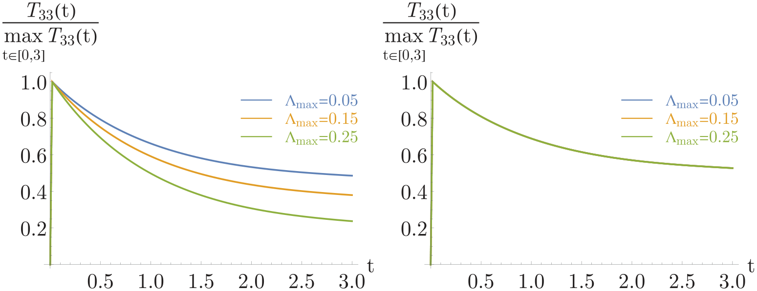
respectively. We skip here the mathematical details associated with deriving equations (72) and (73), which can be found in Appendix 1. The normal stress $T_{33}(t)$ is the stress component perpendicular to the direction of shear and is therefore associated with the Poynting effect. We recall that the Poynting effect is a non-linear phenomenon, whereby the sheared material tends to either expand or contract in the direction perpendicular to the direction of shear. If the material tends to expand, the normal stress $T_{33}(t)$ is negative and a compressive force is required in order to maintain the deformation. Vice-versa, if the material tends to compress vertically, then $T_{33}(t)$ is positive and a tensile force is required to shear the material. In perpendicular shear, the fibres are stretched and rotate. Since the fibres are much stiffer than the isotropic matrix, they generate a vertical compression, which in turn results in a negative Poynting effect [24]. In Figure 4, we plot the relaxation curves for the normal (left) and shear (right) stresses for the MQLV model written with respect to $\mathbf{m}$ (solid lines) and $\hat{\mathbf{m}}$ (dashed lines). First, we note that in perpendicular shear, both versions of the MQLV model predict strain-dependent relaxation. The higher the level of shear, the more significant the relaxation. Moreover, the MQLV model written with respect to the vector $\mathbf{m}$ predicts a more significant relaxation than the MQLV model written with respect to $\hat{\mathbf{m}}$ . This is a direct consequence of the fact that in perpendicular shear, the fibres stretch and rotate in the ${\mathbf{e}}_1-{\mathbf{e}}_3$ plane. However, the vector $\mathbf{m}$ accounts for both the stretching and rotation of the fibres, whereas the vector $\hat{\mathbf{m}}$ only accounts for the rotation of the fibres and is unaffected by the stretching.

Figure 3.

Uni-axial elongation. Normalised stress relaxation curves for the stress $T_{33}(t)$ using the MQLV formulation written with respect to $\mathbf{m}$ (left) and $\hat{\mathbf{m}}$ (right) at different level of strain ${\mathrm{\Lambda }}_{\max }=\{0.05,0.15,0.25\}$ . The curves are plotted using equations (70) and (71), respectively. The stretch $\mathrm{\Lambda }(t)$ is in the form of a ramp function. The following parameters are fixed: the ramp time $t_1=0.02\mathrm{s}$ , the Mooney–Rivlin parameter ${\alpha }_{\mathrm{MR}}=1$ , the elastic moduli $E_l=75$ , ${\mu }_l=5$ , and ${\mu }_t=1$ , the long-term moduli $E_{l\infty }=0.5$ , ${\mu }_{l\infty }=0.8$ , and ${\mu }_{t\infty }=0.9$ , and the characteristic times ${\tau }_{\mathcal{R}}=1$ , ${\tau }_6=1$ , and ${\tau }_5=1$ .

Figure 4.

Perpendicular shear. Normalised stress relaxation curves for the normal (left) and shear (right) stresses $T_{33}(t)$ and $T_{13}(t)$ , respectively, at different level of shear ${\kappa }_{\max }=\{0.1,0.4,0.6\}$ . The solid curves are plotted using equations (72) and (73), which are obtained from the version of the MQLV model where the bases are written with respect to the vector $\mathbf{m}$ . The dashed curves are plotted using equations (93) and (94) with the bases written with respect to the vector $\hat{\mathbf{m}}$ . The amount of shear ${\kappa }_3(t)$ is in the form of a ramp function.The following parameters are fixed: the ramp time $t_1=0.02\mathrm{s}$ , the Mooney–Rivlin parameter ${\alpha }_{\mathrm{MR}}=1$ , the elastic moduli $E_l=75$ , ${\mu }_l=5$ , and ${\mu }_t=1$ , the long-term moduli $E_{l\infty }=0.5$ , ${\mu }_{l\infty }=0.8$ , and ${\mu }_{t\infty }=0.9$ , and the characteristic times ${\tau }_{\mathcal{R}}=1$ , ${\tau }_6=1$ , and ${\tau }_5=1$ .

6. Conclusion

The theory of quasi-linear viscoelasticity has been criticised in the past for its limitations, in particular for failing to capture the non-linearities associated with strain-dependent relaxation and stress-dependent creep. In this paper, we have investigated a modified formulation of the QLV theory for TI materials that accounts for strain-dependent relaxation. The key feature of our model is the linear decomposition of the tensorial relaxation function $\mathbb{G}$ into the sum of scalar components associated with a set of fourth-order tensorial bases. The scalar components are the relaxation functions inherited from the linear viscoelastic theory. We have shown that the set of bases must satisfy the property of additive symmetry in order for the constitutive equation to recover the elastic limit. We have proposed a robust method to identify such a set of bases both for isotropic and TI materials. For fibre-reinforced TI materials, the bases naturally depend on the deformation through the fibre vector. We have discussed two alternative formulations. The first uses the bases with respect to the normalised deformed fibre vector $m(t)$ . In the second version, we write the bases with respect to the deformed vector $\hat{\mathbf{m}}(t)$ . Finally, we have shown that the two models are able to capture strain-dependent relaxation, opening the way towards a fully non-linear viscoelastic theory.