Derivation of an elastic shell model of order h n as n tends to infinity

Abstract

Starting from three-dimensional linear elasticity and performing the dimensional reduction by integration over the thickness, we derive a general form of the areal strain energy density for elastic shells. To obtain the new constitutive model, we do not approximate the deformation fields as polynomials in the thickness coordinate, but rather we keep all terms in the thickness-wise series expansions. As a result, we deduce the explicit form of the shell strain energy density in which the constitutive coefficients are expressed as integrals depending on the thickness h and on the initial curvature. Then, to obtain the shell model of order $O(h^n)$ , we expand the integral coefficients in the strain energy function as power series of h and truncate them to the power $h^n$ . In the case $n=3$ , we recover the classical strain energy density for combined bending and stretching of linear shells, which leads to the Koiter model. Finally, we prove that the proposed shell strain energy function is coercive for any $n\ge 3$ , as well as for the general case $n\to \infty$ .

1. Introduction

The theory of shells is a special chapter of continuum mechanics which investigates the deformation of thin (shell-like) solids. One of the main tasks of shell theory is to establish an appropriate two-dimensional model for such problems, in which the field equations depend on two spatial variables (usually the curvilinear coordinates on the midsurface). These equations should be simple enough to be amenable for practical applications, but also should capture the important features of shell deformation, such as transverse shearing and drilling rotations. Accordingly, there exist several linear and nonlinear models for elastic shells in the literature, having various complexity degrees; some of them are classical and keep only the leading order terms, whereas others are more refined and generalized.

As mentioned in the work by Ball [1], the problem of deriving approximate two-dimensional models from the three-dimensional elasticity to describe the behavior of shells is one of the open problems of elasticity theory. In the past decades, this problem was approached using asymptotic analysis and sharp convergence tools (such as Gamma convergence) by many authors [2, 3, 4, 5]. However, these methods were able to justify the already known pure membrane equations and the inextensional bending equations separately, but they have not given results for a coupled membrane-bending model in general. On the other hand, starting from the three-dimensional elasticity and using a derivation procedure based on integration over the thickness, Steigmann [6] obtained an elastic shell model combining both membrane and bending effects. This general derivation procedure was presented systematically for various shell models by Steigmann [6, 7, 8]; it relies on a thickness-wise expansion of the strain energy and of the deformation field truncated at third order, see an extensive account in the work by Steigmann et al. [9].

One of the research directions for improving the shell model is to consider higher-order models, i.e., models of order $O(h^n)$ with $n>3$ . The higher-order shell models are expected to be more accurate for shells with moderate thickness $h$ . In this case, the terms of order $h^5$ , $h^7,\dots$ can play a significant role (they are no longer negligible) and should be taken into account. In our paper, we follow this line of thought; we employ the derivation procedure presented previously by Steigmann [6, 7, 8] to obtain a general linear shell model of order $O(h^n)$ with $n\to \infty$ . We focus our attention to deduce the respective form of the areal strain energy density for elastic shells, since all other field equations (geometrical relations, balance equations, etc.) have the same form as in the classical linear shell theory. To obtain such a constitutive model, we do not express the displacement vector or the three-dimensional strain energy density as polynomial functions of the thickness coordinate, i.e., we do not truncate the thickness-wise Taylor expansions of these fields. Instead, we retain all the terms in these series expansions with respect to the thickness coordinate. As a result, we obtain the explicit form of the areal strain energy density for shells, in which the coefficients are expressed as integrals depending on the thickness $h$ and on the initial curvature of the midsurface. Subsequently, we can write the strain energy density of order $O(h^n)$ , provided that we expand the integral coefficients as power series of $h$ and keep only the terms up to the power $h^n$ . Using some approximations and assumptions for shells (such as the assumption of zero normal stress), we simplify the expressions and reduce the new constitutive model to a relatively simple explicit form. To show that the proposed shell model is well posed, we prove that the energy function is coercive for all values of $n$ , as well as for $n\to \infty$ . The coercivity of the strain energy function is an important property, since it plays a central role in the proof of existence results for shell equations.

We mention that for $n=3$ we recover the corresponding strain energy density for classical linear elastic shells, which reduces under well-known assumptions to the linear Koiter model. Thus, our shell energy function can be seen as a refinement and generalization of the classical linear shell model. We remark that one can find in the literature some proposed shell energy functions of order $O(h^5)$ . For instance, in the case of plates, a potential energy of order $h^5$ is considered in the work by Pruchnicki [10]. For geometrically nonlinear Cosserat elastic shells (or six-parameter shells), the models of order $h^3$ and $h^5$ have been presented in the work by Bîrsan and colleagues [11, 12, 13] and have been analyzed in matrix notation in the work by Ghiba et al. [14, 15], where the existence of minimizers has been proved. Other approaches to higher-order shell models, including also numerical treatment, have been presented in the previous works [16, 17, 18], among others.

1.1. Outline of the paper

In Section 2, we present briefly the geometrical and kinematical relations for linear elastic shells, including the differential geometry of the reference midsurface and the strain measures. In Section 3, we derive the general expression of the two-dimensional strain energy density for shells made of isotropic and homogeneous materials. Thus, we start from a three-dimensional shell-like body and proceed by integration over the thickness. The dimensional reduction procedure involves some special approximations for thin shells, which lead to a simplified reduced form of the shell strain energy density. The coefficients of the strain energy function are expressed as integrals depending on the thickness $h$ , as well as on the mean curvature $H$ and the Gauss curvature $K$ of the initial configuration. If we develop these coefficients as power series of $h$ and keep only the terms up to the power $h^n$ , then we obtain a shell model of order $O(h^n)$ , for any odd integer $n\ge 3$ , see Section 4. In Section 5, we show that the strain energy function is coercive for the general linear shell model (as $n\to \infty$ ). Moreover, we prove that the coercivity property also holds for the shell model of order $O(h^n)$ , for all $n\ge 3$ .

1.2. Summary of notations

We present first some useful notations which will be used throughout this paper. The Latin indices $i,j,k,\dots$ range over the set $\{1,2,3\}$ , while the Greek indices $\alpha ,\beta ,\gamma ,\dots$ range over the set $\{1,2\}$ . The Einstein summation convention over repeated indices is used. A subscript comma preceding an index $\alpha$ designates partial differentiation with respect to the variable ${\theta }_{\alpha }$ , e.g., $f{,}_{\alpha }=\frac{\partial f}{\partial {\theta }_{\alpha }}$ . We denote by ${\delta }_i^j$ the Kronecker symbol, i.e., ${\delta }_i^j=1$ for $i=j$ , while ${\delta }_i^j=0$ for $i\ne j$ .

We employ the direct tensor notation. Thus, ⊗ designates the dyadic product and $\mathit{I}$ is the identity second-order tensor in the 3-space. Let $\mathrm{tr}(\mathit{X})$ denote the trace of any second-order tensor $\mathit{X}$ . The symmetric part and the deviatoric part of $\mathit{X}$ are defined by $\mathrm{sym}\mathit{X}=\frac{1}{2}(\mathit{X}+{\mathit{X}}^T)$ and $\mathrm{de}{\mathrm{v}}_3\mathit{X}=\mathit{X}-\frac{1}{3}(\mathrm{tr}\mathit{X})\mathit{I}$ , respectively. The scalar product between any second-order tensors $\mathit{X}$ and $\mathit{Y}$ is denoted by $\mathit{X}·\mathit{Y}=\mathrm{tr}({\mathit{X}}^T\mathit{Y})$ . For any vector $\mathit{v}$ and second-order tensor $\mathit{X}$ we denote for convenience $\mathit{vX}:={\mathit{X}}^T\mathit{v}$ .

2. Geometrical and kinematical relations for linear shells

Let us consider the reference configuration $\mathcal{K}$ of a shell-like body with curved midsurface $\mathrm{\Omega }$ and constant thickness $h$ . The convected curvilinear coordinates on $\mathrm{\Omega }$ are denoted by $({\theta }^1,{\theta }^2)$ , the unit normal vector to the surface $\mathrm{\Omega }$ is $\mathit{n}({\theta }^{\alpha })$ and the thickness coordinate along $\mathit{n}$ is designated by $\zeta$ . Thus, the position vector of a generic point of the shell-like body can be written as

$$\mathit{x}({\theta }^{\alpha },\zeta )=\mathit{r}({\theta }^{\alpha })+\zeta \mathit{n}({\theta }^{\alpha }),-\frac{h}{2}\le \zeta \le \frac{h}{2},$$

(1)

where $\mathit{r}({\theta }^{\alpha })$ stands for the position vector of points on the midsurface $\mathrm{\Omega }$ . Let ${\mathit{a}}_{\alpha }={\mathit{r}}_{,\alpha }$ be the covariant base vectors and ${\mathit{a}}^{\alpha }$ the contravariant base vectors such that ${\mathit{a}}^{\alpha }·{\mathit{a}}_{\beta }={\delta }_{\beta }^{\alpha }$ (the Kronecker symbol). We take ${\mathit{a}}_3={\mathit{a}}^3=\mathit{n}$ for convenience.

Let us recall briefly some known shell relations which will be useful in the sequel. The first fundamental tensor $\mathit{1}$ (metric tensor) and the second fundamental tensor $\mathit{k}$ (curvature tensor) of the midsuface $\mathrm{\Omega }$ are given by

$$\begin{array}{c}\mathbb{1}:=\nabla \mathit{r}={\mathit{a}}_{\alpha }\otimes {\mathit{a}}^{\alpha }=a_{\alpha \beta }{\mathit{a}}^{\alpha }\otimes {\mathit{a}}^{\beta }=a^{\alpha \beta }{\mathit{a}}_{\alpha }\otimes {\mathit{a}}_{\beta },\hfill \\ \multicolumn{1}{c}{\mathit{\kappa }:=-\nabla \mathit{n}=-{\mathit{n}}_{,\alpha }\otimes {\mathit{a}}^{\alpha }={\kappa }_{\alpha \beta }{\mathit{a}}^{\alpha }\otimes {\mathit{a}}^{\beta }={\kappa }_{\beta }^{\alpha }{\mathit{a}}_{\alpha }\otimes {\mathit{a}}^{\beta },}\end{array}$$

(2)

where $a_{\alpha \beta }={\mathit{a}}_{\alpha }·{\mathit{a}}_{\beta }$ and ${\kappa }_{\alpha \beta }=-{\mathit{a}}_{\alpha }·{\mathit{n}}_{,\beta }$ are symmetric. Here, ∇ denotes the surface gradient operator given by $\nabla \mathit{f}:=\mathit{f}{,}_{\alpha }\otimes {\mathit{a}}^{\alpha }$ for any field $\mathit{f}$ . Let $a:=\det (a_{\alpha \beta }{)}_{2\times 2}>0$ .

The identity tensor $\mathit{I}$ of the 3-space can be decomposed as

$$\mathit{I}=\mathbb{1}+\mathit{n}\otimes \mathit{n},$$

(3)

so $\mathbb{1}$ can also be regarded as the projection tensor on the tangent plane of $\mathrm{\Omega }$ . Denote by ${\mathcal{T}}_p$ the set of all tensors in the tangent plane, i.e., the set of all second-order tensors $\mathit{S}$ of the form $\mathit{S}=S_{\alpha \beta }{\mathit{a}}^{\alpha }\otimes {\mathit{a}}^{\beta }$ . We see that the tensors $\mathbb{1}$ and $\mathit{\kappa }$ are elements of the linear space ${\mathcal{T}}_p$ , and that $\mathbb{1}$ plays the role of the identity tensor in the space ${\mathcal{T}}_p$ . Indeed, for any tensor $\mathit{S}\in {\mathcal{T}}_p$ we have $\mathbb{1}\mathit{S}=\mathit{S}1=\mathit{S}$ .

Let $H=\frac{1}{2}\mathrm{tr}\mathit{\kappa }=\frac{1}{2}{\kappa }_{\alpha }^{\alpha }$ be the mean curvature and $K=\det \mathit{\kappa }=\det ({\kappa }_{\beta }^{\alpha }{)}_{2\times 2}$ the Gauss curvature of the midsurface $\mathrm{\Omega }$ . Then, we have the following relation of Cayley–Hamilton type:

$${\mathit{\kappa }}^2-2H\mathit{\kappa }+K\mathbb{1}=0.$$

(4)

Consider the cofactor tensor ${\mathit{\kappa }}^{*}$ in ${\mathcal{T}}_p$ given by

$${\mathit{\kappa }}^{*}:=2H\mathbb{1}-\mathit{\kappa },\mathrm{with}\mathit{\kappa }{\mathit{\kappa }}^{*}={\mathit{\kappa }}^{*}\mathit{\kappa }=K\mathbb{1}.$$

(5)

We introduce the tensors $\mathit{\mu }$ and ${\mathit{\mu }}^{-1}$ by

$$\mathit{\mu }:=\nabla \mathit{x}=\mathbb{1}-\zeta \mathit{\kappa }\mathrm{and}{\mathit{\mu }}^{-1}:=\frac{1}{b}(\mathbb{1}-\zeta {\mathit{\kappa }}^{*}),\mathrm{with}b:=1-2H\zeta +K{\zeta }^2,$$

(6)

such that

$$\mathit{\mu }{\mathit{\mu }}^{-1}={\mathit{\mu }}^{-1}\mathit{\mu }=\mathbb{1}.$$

(7)

The Christoffel symbols of the reference midsurface are characterized by

$${{\mathit{a}}^{\alpha }}_{,\beta }=-{\mathrm{\Gamma }}_{\gamma \beta }^{\alpha }{\mathit{a}}^{\gamma }+b_{\beta }^{\alpha }\mathit{n},\mathrm{i}.\mathrm{e}.,{\mathrm{\Gamma }}_{\gamma \beta }^{\alpha }={\mathit{a}}^{\alpha }·{\mathit{a}}_{\gamma ,\beta }.$$

(8)

Let $\mathit{u}({\theta }^{\alpha })$ designate the displacement vector of points on the midsurface,

$$\mathit{u}={\mathit{r}}^{\prime }-\mathit{r},$$

(9)

where ${\mathit{r}}^{\prime }$ is the position vector of the deformed midsurface. The following well-known tensors are measures of distorsion for the midsurface

$${\epsilon }_{\alpha \beta }=\frac{1}{2}(a_{\alpha \beta }^{\prime }-a_{\alpha \beta }),{\rho }_{\alpha \beta }={\kappa }_{\alpha \beta }^{\prime }-{\kappa }_{\alpha \beta },S_{\alpha \beta }^{\lambda }={\mathrm{\Gamma }}_{\alpha \beta }^{\lambda }-{\mathrm{\Gamma }}_{\alpha \beta }^{\lambda },$$

(10)

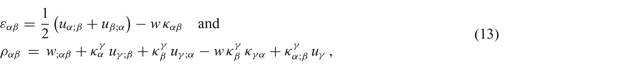
where $a_{\alpha \beta }^{\prime }$ designates the metric, ${\kappa }_{\alpha \beta }^{\prime }$ the curvature tensor, and ${\mathrm{\Gamma }}_{\alpha \beta }^{\lambda }$ the Christoffel symbols in the deformed configuration. Then, the change of metric tensor $\mathit{\epsilon }={\epsilon }_{\alpha \beta }{\mathit{a}}^{\alpha }\otimes {\mathit{a}}^{\beta }$ (also called the infinitesimal surface strain) and the change of curvature tensor $\mathit{\rho }={\rho }_{\alpha \beta }{\mathit{a}}^{\alpha }\otimes {\mathit{a}}^{\beta }$ (bending measure) are given by

$${\epsilon }_{\alpha \beta }=\frac{1}{2}({\mathit{u}}_{,\alpha }·{\mathit{a}}_{\beta }+{\mathit{u}}_{,\beta }·{\mathit{a}}_{\alpha })\mathrm{and}{\rho }_{\alpha \beta }=\mathit{n}·{\mathit{u}}_{;\alpha \beta },$$

(11)

where ${\mathit{u}}_{;\alpha \beta }={\mathit{u}}_{,\alpha \beta }-{\mathit{u}}_{,\lambda }{\mathrm{\Gamma }}_{\alpha \beta }^{\lambda }$ . If we denote the components of the displacement vector by

$$\mathit{u}=u_{\alpha }{\mathit{a}}^{\alpha }+w\mathit{n},$$

(12)

then it holds (see e.g., Steigmann et al. [9])

$$\begin{array}{c}{\epsilon }_{\alpha \beta }=\frac{1}{2}(u_{\alpha ;\beta }+u_{\beta ;\alpha })-w{\kappa }_{\alpha \beta }\mathrm{and}\hfill \\ \multicolumn{1}{c}{{\rho }_{\alpha \beta }=w_{;\alpha \beta }+{\kappa }_{\alpha }^{\gamma }{u}_{\gamma ;\beta }+{\kappa }_{\beta }^{\gamma }{u}_{\gamma ;\alpha }-w{\kappa }_{\beta }^{\gamma }{\kappa }_{\gamma \alpha }+{\kappa }_{\alpha ;\beta }^{\gamma }{u}_{\gamma },}\end{array}$$

(13)

where the covariant derivatives are

$$\begin{array}{c}{u}_{\gamma ;\alpha }=u_{\gamma ,\alpha }-u_{\lambda }{\mathrm{\Gamma }}_{\alpha \gamma }^{\lambda },w_{;\alpha \beta }=w_{,\alpha \beta }-w_{,\gamma }{\mathrm{\Gamma }}_{\alpha \beta }^{\gamma }\hfill \\ \multicolumn{1}{c}{\mathrm{and}{\kappa }_{\alpha ;\beta }^{\gamma }={\kappa }_{\alpha ,\beta }^{\gamma }+{\kappa }_{\alpha }^{\lambda }{\mathrm{\Gamma }}_{\lambda \beta }^{\gamma }-{\kappa }_{\lambda }^{\gamma }{\mathrm{\Gamma }}_{\alpha \beta }^{\lambda }.}\end{array}$$

(14)

Both tensors $\mathit{\epsilon }$ and $\mathit{\rho }$ are symmetric. From equation (12) it follows that

$$\nabla \mathit{u}=(u_{\alpha ;\beta }-w{\kappa }_{\alpha \beta }){\mathit{a}}^{\alpha }\otimes {\mathit{a}}^{\beta }+(w_{,\beta }+u_{\alpha }{\kappa }_{\beta }^{\alpha })\mathit{n}\otimes {\mathit{a}}^{\beta },$$

(15)

so we have

$$\mathit{\epsilon }=\mathrm{sym}(\mathbb{1}\nabla \mathit{u}).$$

(16)

Let us denote by $\mathit{\alpha }$ the vector

$$\mathit{\alpha }:=-\mathit{n}\nabla \mathit{u}=-(w_{,\beta }+u_{\alpha }{\kappa }_{\beta }^{\alpha }){\mathit{a}}^{\beta }=-(\nabla w+\mathit{\kappa }\mathit{u}).$$

(17)

Using the vector field $\mathit{\alpha }$ , we can express the tensor ${\rho }_{\alpha \beta }$ as follows

$${\rho }_{\gamma \beta }=-{\alpha }_{\gamma ;\beta }+{\kappa }_{\beta }^{\lambda }(u_{\lambda ;\gamma }-w{\kappa }_{\lambda \gamma }).$$

(18)

Moreover, the following relation holds (see Steigmann et al. [9]):

$${\mathit{u}}_{;\alpha \beta }=S_{\alpha \beta }^{\lambda }{\mathit{a}}_{\lambda }+{\kappa }_{\alpha \beta }\mathit{\alpha }+{\rho }_{\alpha \beta }\mathit{n},$$

(19)

so the change of Christoffel symbols is expressed by

$$S_{\alpha \beta }^{\gamma }={\mathit{a}}^{\gamma }·({\mathit{u}}_{;\alpha \beta }-{\kappa }_{\alpha \beta }\mathit{\alpha }).$$

(20)

In view of the above relations, one can show that

$$S_{\alpha \beta }^{\alpha }=(\mathrm{tr}\mathit{\epsilon }{)}_{,\beta },$$

(21)

so we have

$$\nabla [(\mathrm{tr}\mathit{\epsilon })\mathit{n}]=-(\mathrm{tr}\mathit{\epsilon })\mathit{\kappa }+S_{\alpha \beta }^{\alpha }\mathit{n}\otimes {\mathit{a}}^{\beta }.$$

(22)

Note that $S_{\alpha \beta }^{\gamma }$ can be expressed as a combination of the covariant derivatives of the strain tensor ${\epsilon }_{\alpha \beta }$ by the following relation:

$$S_{\alpha \beta }^{\lambda }=a^{\lambda \gamma }({\epsilon }_{\gamma \alpha ;\beta }+{\epsilon }_{\gamma \beta ;\alpha }-{\epsilon }_{\alpha \beta ;\gamma }),$$

(23)

where ${\epsilon }_{\alpha \beta ;\gamma }={\epsilon }_{\alpha \beta ,\gamma }-{\epsilon }_{\beta \lambda }{\mathrm{\Gamma }}_{\alpha \gamma }^{\lambda }-{\epsilon }_{\alpha \lambda }{\mathrm{\Gamma }}_{\beta \gamma }^{\lambda }$ .

Remark: In what follows, we consider isotropic and homogeneous elastic shells characterized by the Lamé constants $\lambda$ and $\mu$ . Let us denote by $W_s$ the bilinear form

$$W_s(\mathit{X},\mathit{Y}):=\mu \mathrm{sym}(\mathbb{1}\mathit{X})·\mathrm{sym}(\mathbb{1}\mathit{Y})+\frac{\lambda \mu }{\lambda +2\mu }(\mathrm{tr}\mathit{X})(\mathrm{tr}\mathit{Y}),$$

(24)

defined for any tensors of the form $\mathit{X}=X_{i\alpha }{\mathit{a}}^i\otimes {\mathit{a}}^{\alpha }$ , $\mathit{Y}=Y_{i\alpha }{\mathit{a}}^i\otimes {\mathit{a}}^{\alpha }$ . The associated quadratic form is

$$W_s(\mathit{X}):=W_s(\mathit{X},\mathit{X})=\mu \parallel \mathrm{sym}(\mathbb{1}\mathit{X}){\parallel }^2+\frac{\lambda \mu }{\lambda +2\mu }(\mathrm{tr}\mathit{X}{)}^2.$$

(25)

Then, in the classical linear theory of shells (Koiter), the areal strain energy density is expressed as a function of $\mathit{\epsilon }$ and $\mathit{\rho }$ in the form (see literature [6, 7, 8, 19, 20])

$$W_{\mathrm{Koit}}(\mathit{\epsilon },\mathit{\rho })=h{W}_s(\mathit{\epsilon })+\frac{h^3}{12}{W}_s(\mathit{\rho }).$$

(26)

3. Derivation of the two-dimensional shell energy density

Let $\tilde{\mathit{u}}(\mathit{X})$ be the three-dimensional displacement field of the shell-like body and $\tilde{\mathit{H}}(\mathit{X})$ be its gradient. We employ carets to denote the same fields written as functions of the coordinates $({\theta }^{\alpha },\zeta )$ , i.e.,

$$\hat{\mathit{u}}({\theta }^{\alpha },\zeta ):=\tilde{\mathit{u}}(\mathit{r}({\theta }^{\alpha })+\zeta \mathit{n}({\theta }^{\alpha })),\hat{\mathit{H}}({\theta }^{\alpha },\zeta ):=\tilde{\mathit{H}}(\mathit{r}({\theta }^{\alpha })+\zeta \mathit{n}({\theta }^{\alpha })).$$

(27)

For an isotropic and homogeneous elastic material with Lamé constants $\lambda$ and $\mu$ , the tensor of elastic moduli $\underset{¯}{\mathit{C}}$ is given by

$$\underset{¯}{\mathit{C}}[\mathit{T}]=2\mu \mathrm{sym}\mathit{T}+\lambda (\mathrm{tr}\mathit{T})\mathit{I}\mathrm{for}\mathrm{any}\mathit{T},$$

(28)

and the strain energy density is

$$U=\frac{1}{2}\hat{\mathit{H}}·\underset{¯}{\mathit{C}}[\hat{\mathit{H}}]=\mu \parallel \mathrm{sym}\hat{\mathit{H}}{\parallel }^2+\frac{\lambda }{2}(\mathrm{tr}\hat{\mathit{H}}{)}^2.$$

(29)

Let us denote by $W_{3\mathrm{d}}(\mathit{X},\mathit{Y})$ the bilinear form

$$W_{3\mathrm{d}}(\mathit{X},\mathit{Y}):=\mu (\mathrm{sym}\mathit{X})·(\mathrm{sym}\mathit{Y})+\frac{\lambda }{2}(\mathrm{tr}\mathit{X})(\mathrm{tr}\mathit{Y})\mathrm{for}\mathrm{any}\mathit{X},\mathit{Y},$$

(30)

and let $W_{3\mathrm{d}}(\mathit{X}):=W_{3\mathrm{d}}(\mathit{X},\mathit{X})$ be the associated quadratic form. Then, the strain energy density (29) can be written as

$$U=W_{3\mathrm{d}}(\hat{\mathit{H}}).$$

(31)

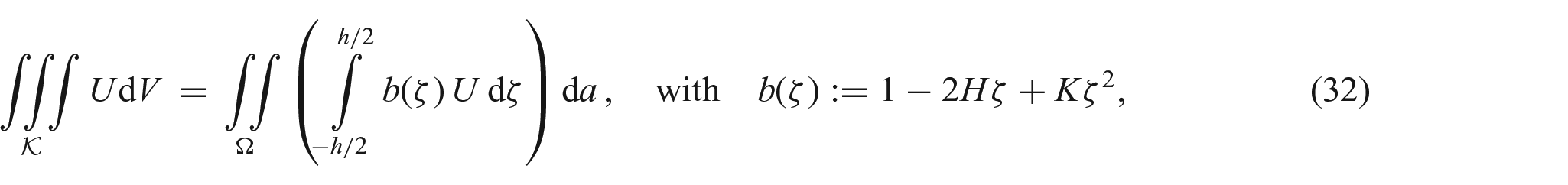
The elastically stored energy of the three-dimensional shell-like body is given by the volume integral

$$\underset{\mathcal{K}}{\int \int \int }U\mathrm{d}V=\int \underset{\mathrm{\Omega }}{\int }(\underset{-h/2}{\overset{h/2}{\int }}b(\zeta )U\mathrm{d}\zeta )\mathrm{d}a,\mathrm{with}b(\zeta ):=1-2H\zeta +K{\zeta }^2,$$

(32)

since the elemental volume $\mathrm{d}V$ and elemental area $\mathrm{d}a$ are expressed by (see Steigmann et al. [9])

$$\mathrm{d}a=\sqrt{a({\theta }^{\alpha })}\mathrm{d}{\theta }^1\mathrm{d}{\theta }^2\mathrm{and}\mathrm{d}V=b(\zeta )\sqrt{a({\theta }^{\alpha })}\mathrm{d}{\theta }^1\mathrm{d}{\theta }^2\mathrm{d}\zeta =b(\zeta )\mathrm{d}a\mathrm{d}\zeta .$$

(33)

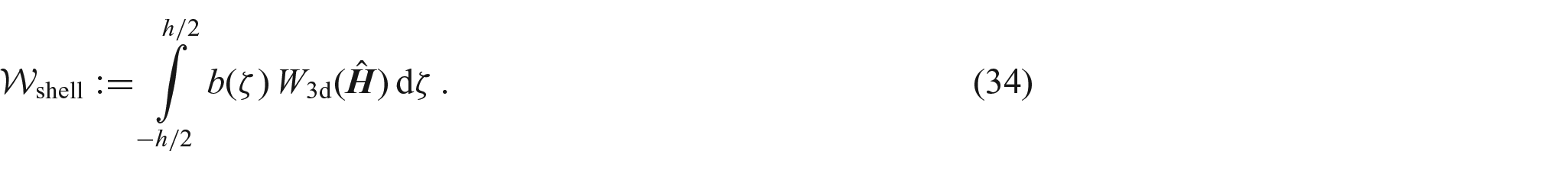
In view of equations (31) and (32), we see that the areal strain energy density of the shell is given by

$${\mathcal{W}}_{\mathrm{shell}}:=\underset{-h/2}{\overset{h/2}{\int }}b(\zeta )W_{3\mathrm{d}}(\hat{\mathit{H}})\mathrm{d}\zeta .$$

(34)

3.1. Gradients of the displacement field

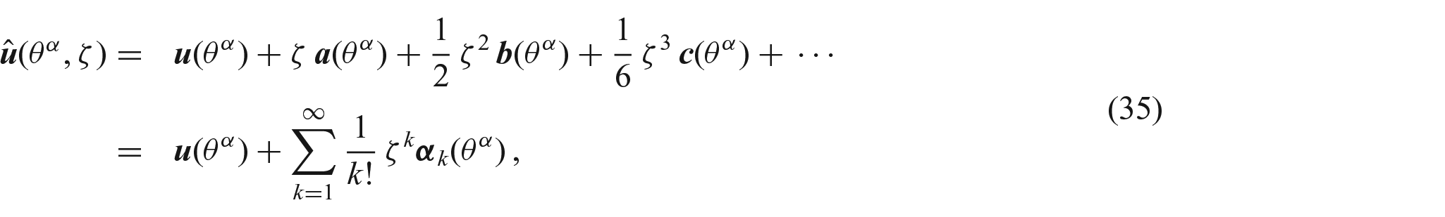
In order to perform the integration over the thickness in equation (34), we develop the displacement field $\hat{\mathit{u}}$ and its gradient $\hat{\mathit{H}}$ as power series of the thickness coordinate $\zeta$ . For any field $\mathit{f}$ , denote for brevity by ${\mathit{f}}_0$ the value of $\mathit{f}$ at $\zeta =0$ . Also, we designate its partial derivatives by ${\mathit{f}}_{,\alpha }:=\frac{\partial \mathit{f}}{\partial {\theta }^{\alpha }}$ and ${\mathit{f}}^{\prime }:=\frac{\partial \mathit{f}}{\partial \zeta }$ . Thus, we can write the expansion

$$\begin{array}{c}\hat{\mathit{u}}({\theta }^{\alpha },\zeta )=\mathit{u}({\theta }^{\alpha })+\zeta \mathit{a}({\theta }^{\alpha })+\frac{1}{2}{\zeta }^2\mathit{b}({\theta }^{\alpha })+\frac{1}{6}{\zeta }^3\mathit{c}({\theta }^{\alpha })+\cdots \hfill \\ \multicolumn{1}{c}{=\mathit{u}({\theta }^{\alpha })+\sum _{k=1}^{\infty }\frac{1}{k!}{\zeta }^k{\mathit{\alpha }}_k({\theta }^{\alpha }),}\end{array}$$

(35)

where $\mathit{u}={\hat{\mathit{u}}}_0$ is the displacement of the midsurface and

$$\mathit{a}={\mathit{\alpha }}_1={{\hat{\mathit{u}}}^{\prime }}_0,\mathit{b}={\mathit{\alpha }}_2={{\hat{\mathit{u}}}^{\prime \prime }}_0,\mathit{c}={\mathit{\alpha }}_3={{\hat{\mathit{u}}}^{\prime \prime \prime }}_0,\mathrm{and}{\mathit{\alpha }}_k={\hat{\mathit{u}}}_0^{(k)}\mathrm{for}k\ge 4.$$

(36)

Similarly, we can develop $\hat{\mathit{H}}$ about $\zeta =0$ in the form

$$\hat{\mathit{H}}({\theta }^{\alpha },\zeta )={\hat{\mathit{H}}}_0({\theta }^{\alpha })+\sum _{k=1}^{\infty }\frac{1}{k!}{\zeta }^k{\hat{\mathit{H}}}_0^{(k)}({\theta }^{\alpha }).$$

(37)

Let us determine the expression of the derivatives ${\hat{\mathit{H}}}_0^{(k)}$ for any $k\ge 0$ . For the three-dimensional displacement gradient $\hat{\mathit{H}}$ , we have the relation (see Steigmann et al. [9])

$$\hat{\mathit{H}}=(\nabla \hat{\mathit{u}}){\mathit{\mu }}^{-1}+{\hat{\mathit{u}}}^{\prime }\otimes \mathit{n}.$$

(38)

Next, we need a formula for the higher derivatives of ${\mathit{\mu }}^{-1}$ . By differentiating the relation $\mathit{\mu }{\mathit{\mu }}^{-1}=\mathbb{1}$ with respect to $\zeta$ , we get ${\mathit{\mu }}^{\prime }{\mathit{\mu }}^{-1}+\mathit{\mu }({\mathit{\mu }}^{-1}{)}^{\prime }=0$ , so we have (since ${\mathit{\mu }}^{\prime }=-\mathit{\kappa }$ )

$$({\mathit{\mu }}^{-1}{)}^{\prime }={\mathit{\mu }}^{-1}\mathit{\kappa }{\mathit{\mu }}^{-1}.$$

Furthermore, we differentiate the last equation and find

$$({\mathit{\mu }}^{-1}{)}^{\prime \prime }=({\mathit{\mu }}^{-1}{)}^{\prime }\mathit{\kappa }{\mathit{\mu }}^{-1}+{\mathit{\mu }}^{-1}\mathit{\kappa }({\mathit{\mu }}^{-1}{)}^{\prime }=2{\mathit{\mu }}^{-1}\mathit{\kappa }{\mathit{\mu }}^{-1}\mathit{\kappa }{\mathit{\mu }}^{-1}=2({\mathit{\mu }}^{-1}\mathit{\kappa }{)}^2{\mathit{\mu }}^{-1}.$$

We can continue this procedure and show by induction that the following formula holds:

$$({\mathit{\mu }}^{-1}{)}^{(n)}=n!({\mathit{\mu }}^{-1}\mathit{\kappa }{)}^n{\mathit{\mu }}^{-1}\mathrm{for}\mathrm{any}n\ge 1.$$

(39)

If we put here $\zeta =0$ and use $({\mathit{\mu }}^{-1}{)}_0=\mathbb{1}$ (cf. equation (6)), we get

$$({\mathit{\mu }}^{-1}{)}_0^{(n)}=n!{\mathit{\kappa }}^n\mathrm{for}\mathrm{any}n\ge 1.$$

(40)

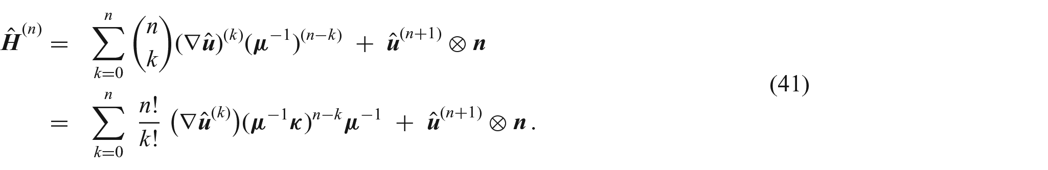
Now differentiating $n$ times relation (38) with respect to $\zeta$ and using equation (39) we find

$$\begin{array}{c}{\hat{\mathit{H}}}^{(n)}=\sum _{k=0}^n\left(\begin{array}{c}n\hfill \\ \multicolumn{1}{c}{k}\end{array}\right){(\nabla \hat{\mathit{u}})}^{(k)}{({\mathit{\mu }}^{-1})}^{(n-k)}+{\hat{\mathit{u}}}^{(n+1)}\otimes \mathit{n}\hfill \\ \multicolumn{1}{c}{=\sum _{k=0}^n\frac{n!}{k!}(\nabla {\hat{\mathit{u}}}^{(k)})({\mathit{\mu }}^{-1}\mathit{\kappa }{)}^{n-k}{\mathit{\mu }}^{-1}+{\hat{\mathit{u}}}^{(n+1)}\otimes \mathit{n}.}\end{array}$$

(41)

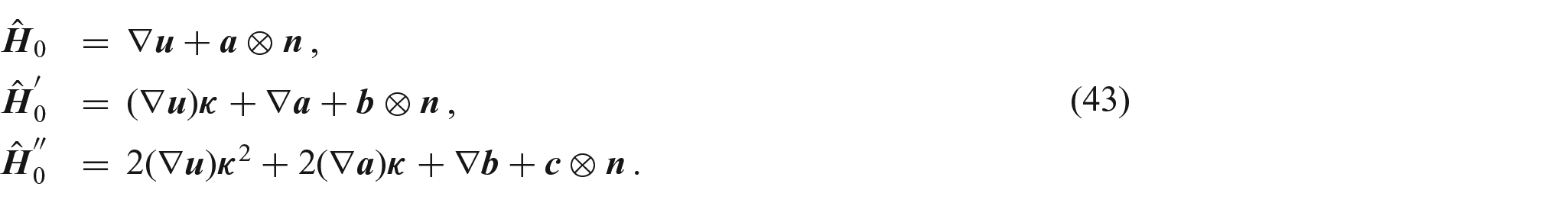
The last relation generalizes relation (38). We take here $\zeta =0$ and obtain

$${\hat{\mathit{H}}}_0^{(n)}=n!(\nabla \mathit{u}){\mathit{\kappa }}^n+(\sum _{k=1}^n\frac{n!}{k!}(\nabla {\mathit{\alpha }}_k){\mathit{\kappa }}^{n-k})+{\mathit{\alpha }}_{n+1}\otimes \mathit{n}.$$

(42)

For the orders $n=0,1,2$ , this general formula reads

$$\begin{array}{c}{\hat{\mathit{H}}}_0=\nabla \mathit{u}+\mathit{a}\otimes \mathit{n},\hfill \\ \multicolumn{1}{c}{{{\hat{\mathit{H}}}^{\prime }}_0=(\nabla \mathit{u})\mathit{\kappa }+\nabla \mathit{a}+\mathit{b}\otimes \mathit{n},}\\ \multicolumn{1}{c}{{{\hat{\mathit{H}}}^{\prime \prime }}_0=2(\nabla \mathit{u}){\mathit{\kappa }}^2+2(\nabla \mathit{a})\mathit{\kappa }+\nabla \mathit{b}+\mathit{c}\otimes \mathit{n}.}\end{array}$$

(43)

3.2. Simplifying assumptions and approximations

We will adopt now some assumptions (specific to shell theory), which allow to simplify relations (37) and (42) and finally to integrate over the thickness.

Let $\mathit{P}$ be the Piola stress tensor given by $\mathit{P}=\underset{¯}{\mathit{C}}[\hat{\mathit{H}}]$ , so we have

$${\mathit{P}}^{(k)}=\underset{¯}{\mathit{C}}[{\hat{\mathit{H}}}^{(k)}]\mathrm{and}{\mathit{P}}_0^{(k)}=\underset{¯}{\mathit{C}}[{\hat{\mathit{H}}}_0^{(k)}].$$

(44)

We assume that the transversal stress vector $\mathit{Pn}$ is very small, such that we can approximate

$${\mathit{P}}_0^{(k)}\mathit{n}\simeq 0\mathrm{for}\mathrm{all}k\ge 0.$$

(45)

These conditions provide equations for the determination of the coefficients $\mathit{a},\mathit{b},\mathit{c},\dots$ (all ${\mathit{\alpha }}_k$ ) in the development (35) in terms of $\mathit{u}$ and its gradients.

Let us prove first the following useful result:

Lemma 1. For any second-order tensor $\mathit{Z}=Z_{\mathrm{ij}}{\mathit{a}}^i\otimes {\mathit{a}}^j$ , we define the tensor $\mathit{P}(\mathit{Z})$ according to equation (28) by

$$\mathit{P}(\mathit{Z})=\underset{¯}{\mathit{C}}[\mathit{Z}]=2\mu \mathrm{sym}\mathit{Z}+\lambda (\mathrm{tr}\mathit{Z})\mathit{I}.$$

(46)

Then, the equation

$$\mathit{P}(\mathit{Z})\mathit{n}=\mathit{0}$$

(47)

is equivalent to

$$\mathit{Zn}=-\mathit{n}(\mathit{Z}\mathbb{1})-\frac{\lambda }{\lambda +2\mu }\mathrm{tr}(\mathit{Z}\mathbb{1})\mathit{n},$$

(48)

which means that

$$\mathit{Z}=L_n(\mathit{Z}\mathbb{1}),$$

(49)

where we have denoted by $L_n$ the linear operator given by

$$L_n(\mathit{X}):=\mathit{X}-[\mathit{nX}+\frac{\lambda }{\lambda +2\mu }(\mathrm{tr}\mathit{X})\mathit{n}]\otimes \mathit{n}\mathrm{for}\mathrm{any}\mathit{X}=X_{i\alpha }{\mathit{a}}^i\otimes {\mathit{a}}^{\alpha }.$$

(50)

Proof. If we decompose $\mathit{Z}=\mathit{Z}\mathbb{1}+(\mathit{Zn})\otimes \mathit{n}$ , then equation (47) can be written successively in the equivalent forms

$$\begin{array}{c}[\mu (\mathit{Zn}\otimes \mathit{n}+\mathit{n}\otimes \mathit{Zn})+\lambda (\mathit{n}·\mathit{Zn})\mathit{I}]\mathit{n}=-\mathit{P}(\mathit{Z}\mathbb{1})\mathit{n},\hfill \end{array}$$

or

$$\mu (\mathit{Zn})+(\lambda +\mu )(\mathit{n}·\mathit{Zn})\mathit{n}=-[\mu (\mathit{Z}\mathbb{1}+\mathbb{1}{\mathit{Z}}^T)+\lambda \mathrm{tr}(\mathit{Z}\mathbb{1})\mathit{I}]\mathit{n},$$

or

$$[\mu \mathbb{1}+(\lambda +2\mu )\mathit{n}\otimes \mathit{n}](\mathit{Zn})=-[\mu \mathbb{1}{\mathit{Z}}^T\mathit{n}+\lambda \mathrm{tr}(\mathit{Z}\mathbb{1})\mathit{n}],$$

or, since $\mu >0$ and $\lambda +2\mu >0$ ,

$$\mathit{Zn}=-[\frac{1}{\mu }\mathbb{1}+\frac{1}{\lambda +2\mu }\mathit{n}\otimes \mathit{n}][\mu \mathit{n}(\mathit{Z}\mathbb{1})+\lambda \mathrm{tr}(\mathit{Z}\mathbb{1})\mathit{n}],$$

so we derive relation (48). Substituting $\mathit{Zn}$ from equation (48) into the representation $\mathit{Z}=\mathit{Z}\mathbb{1}+(\mathit{Zn})\otimes \mathit{n}$ and using notation (50), we obtain the desired result (49). The proof is complete. ■

3.2.1. Determination of the vector fields $\mathit{a}$ , $\mathit{b}$ , and $\mathit{c}$

Equation (45) for $k=0$ can be written as

$${\mathit{P}}_0\mathit{n}=0,\mathrm{i}.\mathrm{e}.,\mathit{P}({\hat{\mathit{H}}}_0)\mathit{n}=0,$$

(51)

and using expression (43)₁ for ${\hat{\mathit{H}}}_0$ we get

$$\mathit{P}(\nabla \mathit{u}+\mathit{a}\otimes \mathit{n})\mathit{n}=0.$$

(52)

We can apply now Lemma 1 for equation (52), and since ${\hat{\mathit{H}}}_0\mathit{n}=\mathit{a}$ , ${\hat{\mathit{H}}}_0\mathbb{1}=\nabla \mathit{u}$ , we obtain

$$\mathit{a}=-\mathit{n}(\nabla \mathit{u})-\frac{\lambda }{\lambda +2\mu }\mathrm{tr}(\nabla \mathit{u})\mathit{n}.$$

(53)

In view of equations (16) and (17), we have $\mathit{n}(\nabla \mathit{u})=-\mathit{\alpha }$ and $\mathrm{tr}(\nabla \mathit{u})=\mathrm{tr}\mathit{\epsilon }$ , so it holds

$$\overline{\mathit{a}}=\mathit{\alpha }-\frac{\lambda }{\lambda +2\mu }(\mathrm{tr}\mathit{\epsilon })\mathit{n}\mathrm{and}{\overline{\mathit{H}}}_0=L_n(\nabla \mathit{u}).$$

(54)

Thus, we have determined the vector $\mathit{a}$ from equation (51) and we denote this solution with $\overline{\mathit{a}}$ , see equation (54). In the following developments, we replace $\mathit{a}$ with $\overline{\mathit{a}}$ and we mark any function expressed with help of $\overline{\mathit{a}}$ by a superposed bar, e.g.,

$${\overline{\mathit{H}}}_0=\nabla \mathit{u}+\overline{\mathit{a}}\otimes \mathit{n}\mathrm{etc}.$$

(55)

Next, to determine the vector $\mathit{b}$ we write equation (45) for $k=1$ in the form

$${\mathit{P}}_0^{\prime }\mathit{n}=0,\mathrm{i}.\mathrm{e}.,\mathit{P}({\overline{\mathit{H}}}_0^{\prime })\mathit{n}=0,\mathrm{with}{\mathit{H}}_0^{\prime }=(\nabla \mathit{u})\mathit{\kappa }+\nabla \overline{\mathit{a}}+\mathit{b}\otimes \mathit{n},$$

(56)

cf. equation (43). Let us introduce the tensor $\overline{\mathit{B}}$ given by

$$\overline{\mathit{B}}=(\nabla \mathit{u})\mathit{\kappa }+\nabla \overline{\mathit{a}},$$

(57)

such that we have ${\overline{\mathit{H}}}_0^{\prime }\mathbb{1}=\overline{\mathit{B}}$ and ${\overline{\mathit{H}}}_0^{\prime }\mathit{n}=\mathit{b}$ . Hence, applying Lemma 1 for equation (56), we determine the vector $\mathit{b}$ in the form

$$\overline{\mathit{b}}=-\mathit{n}\overline{\mathit{B}}-\frac{\lambda }{\lambda +2\mu }(\mathrm{tr}\overline{\mathit{B}})\mathit{n}\mathrm{and}{\overline{\mathit{H}}}_0^{\prime }=L_n(\overline{\mathit{B}}).$$

(58)

Notice that the tensor $\overline{\mathit{B}}$ defined by equation (57) can be expressed in terms of the bending measure $\mathit{\rho }$ and the strain tensor $\mathit{\epsilon }$ by the following equation:

$$\overline{\mathit{B}}=-\mathit{\rho }+2\mathit{\epsilon }\mathit{\kappa }-\frac{\lambda }{\lambda +2\mu }\nabla [(\mathrm{tr}\mathit{\epsilon })\mathit{n}].$$

(59)

To prove this relation, we use equation (54)₁ and write

$$\begin{array}{c}\overline{\mathit{B}}=\nabla \overline{\mathit{a}}+(\nabla \mathit{u})\mathit{\kappa }=\nabla [\mathit{\alpha }-\frac{\lambda }{\lambda +2\mu }(\mathrm{tr}\mathit{\epsilon })\mathit{n}]+({\mathit{u}}_{,\alpha }\otimes {\mathit{a}}^{\alpha })({\kappa }_{\beta }^{\gamma }{\mathit{a}}_{\gamma }\otimes {\mathit{a}}^{\beta })\hfill \\ ={\mathit{\alpha }}_{,\beta }\otimes {\mathit{a}}^{\beta }+{\kappa }_{\beta }^{\alpha }{\mathit{u}}_{,\alpha }\otimes {\mathit{a}}^{\beta }-\frac{\lambda }{\lambda +2\mu }\nabla [(\mathrm{tr}\mathit{\epsilon })\mathit{n}].\hfill \end{array}$$

(60)

Furthermore, from relations (17), (18), and (13)₁ we get

$$\begin{array}{c}{\mathit{\alpha }}_{,\beta }\otimes {\mathit{a}}^{\beta }+{\kappa }_{\beta }^{\alpha }{\mathit{u}}_{,\alpha }\otimes {\mathit{a}}^{\beta }=({\alpha }_{\alpha ;\beta }{\mathit{a}}^{\alpha }+{\kappa }_{\beta }^{\alpha }{\alpha }_{\alpha }\mathit{n})\otimes {\mathit{a}}^{\beta }+{\kappa }_{\beta }^{\alpha }[(u_{\gamma ;\alpha }-w{\kappa }_{\alpha \gamma }){\mathit{a}}^{\gamma }+(w_{,\alpha }+{\kappa }_{\alpha }^{\gamma }{u}_{\gamma })\mathit{n}]\otimes {\mathit{a}}^{\beta }\hfill \\ =[{\alpha }_{\alpha ;\beta }+{\kappa }_{\beta }^{\gamma }(u_{\alpha ;\gamma }-w{\kappa }_{\alpha \gamma })]{\mathit{a}}^{\alpha }\otimes {\mathit{a}}^{\beta }\hfill \\ =[{\alpha }_{\alpha ;\beta }-{\kappa }_{\beta }^{\gamma }(u_{\gamma ;\alpha }-w{\kappa }_{\alpha \gamma })]{\mathit{a}}^{\alpha }\otimes {\mathit{a}}^{\beta }+{\kappa }_{\beta }^{\gamma }(u_{\alpha ;\gamma }+u_{\gamma ;\alpha }-2w{\kappa }_{\alpha \gamma }){\mathit{a}}^{\alpha }\otimes {\mathit{a}}^{\beta }\hfill \\ =-\mathit{\rho }+2\mathit{\epsilon }\mathit{\kappa }.\hfill \end{array}$$

(61)

Substituting equation (61) into equation (60), we deduce that relation (59) holds true.

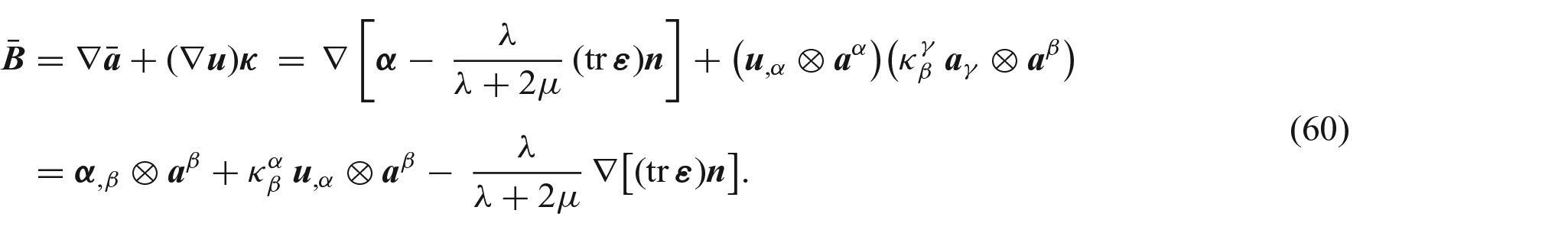
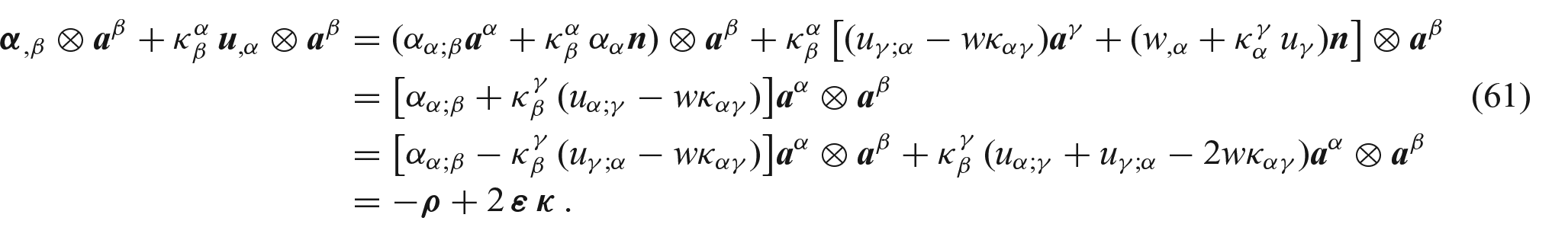
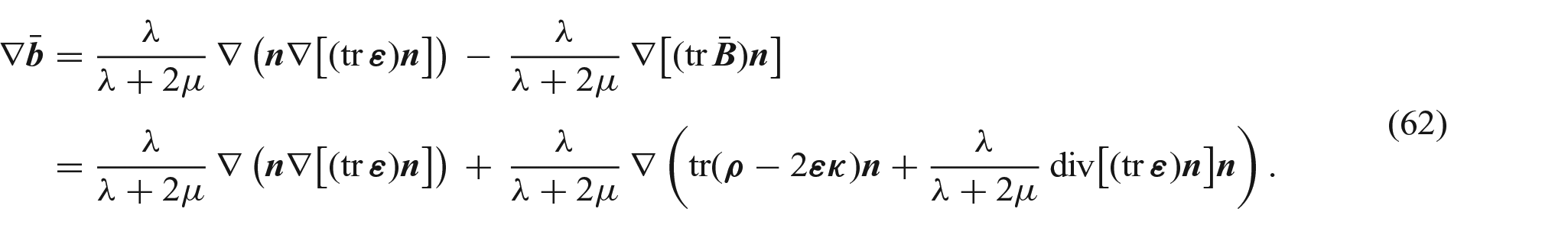
Let us approximate now the gradient of $\mathit{b}$ . From equations (58)₁ and (59) it follows

$$\begin{array}{c}\nabla \overline{\mathit{b}}=\frac{\lambda }{\lambda +2\mu }\nabla (\mathit{n}\nabla [(\mathrm{tr}\mathit{\epsilon })\mathit{n}])-\frac{\lambda }{\lambda +2\mu }\nabla [(\mathrm{tr}\overline{\mathit{B}})\mathit{n}]\hfill \\ =\frac{\lambda }{\lambda +2\mu }\nabla (\mathit{n}\nabla [(\mathrm{tr}\mathit{\epsilon })\mathit{n}])+\frac{\lambda }{\lambda +2\mu }\nabla (\mathrm{tr}(\mathit{\rho }-2\mathit{\epsilon }\mathit{\kappa })\mathit{n}+\frac{\lambda }{\lambda +2\mu }\mathrm{div}[(\mathrm{tr}\mathit{\epsilon })\mathit{n}]\mathit{n}).\hfill \end{array}$$

(62)

In this model, we do not take into account the gradients of the strain tensors $\mathit{\epsilon }$ and $\mathit{\rho }$ . Then, in view of the above relation, we can neglect the gradient of $\overline{\mathit{b}}$ , i.e., we approximate

$$\nabla \overline{\mathit{b}}\simeq 0.$$

(63)

We can proceed similarly for the determination of the vector field $\mathit{c}$ : using the approximation (63) in relation (43)₃ we get

$${{\overline{\mathit{H}}}^{\prime \prime }}_0=2(\nabla \mathit{u}){\mathit{\kappa }}^2+2(\nabla \overline{\mathit{a}})\mathit{\kappa }+\mathit{c}\otimes \mathit{n}=2\overline{\mathit{B}}\mathit{\kappa }+\mathit{c}\otimes \mathit{n}.$$

(64)

Equation (45) for $k=2$ reads

$${\mathit{P}}_0^{\prime \prime }\mathit{n}=0,\mathrm{i}.\mathrm{e}.,\mathit{P}(2\overline{\mathit{B}}\mathit{\kappa }+\mathit{c}\otimes \mathit{n})\mathit{n}=0.$$

(65)

Using Lemma 1, from the last equation we obtain

$$\overline{\mathit{c}}=-2\mathit{n}(\overline{\mathit{B}}\mathit{\kappa })-\frac{\lambda }{\lambda +2\mu }2\mathrm{tr}(\overline{\mathit{B}}\mathit{\kappa })\mathit{n}\mathrm{and}{{\overline{\mathit{H}}}^{\prime \prime }}_0=2L_n(\overline{\mathit{B}}\mathit{\kappa }).$$

(66)

Since we do not take into account the gradients of $\mathit{\epsilon }$ and $\mathit{\rho }$ in our model, then we can approximate

$$\nabla \overline{\mathit{c}}=\frac{2\lambda }{\lambda +2\mu }\nabla (\mathit{n}\nabla [(\mathrm{tr}\mathit{\epsilon })\mathit{n}]\mathit{\kappa })-\frac{2\lambda }{\lambda +2\mu }\nabla [\mathrm{tr}(\overline{\mathit{B}}\mathit{\kappa })\mathit{n}]\simeq 0,$$

(67)

i.e., we neglect the gradient of $\overline{\mathit{c}}$ .

3.2.2. Determination of all vector fields ${\mathit{\alpha }}_k$ (induction procedure)

Let us prove by mathematical induction that the following relations hold for any order $n\ge 1$ :

$$\begin{array}{c}{\mathit{\alpha }}_{n+1}=-n![\mathit{n}(\overline{\mathit{B}}{\mathit{\kappa }}^{n-1})+\frac{\lambda }{\lambda +2\mu }\mathrm{tr}(\overline{\mathit{B}}{\mathit{\kappa }}^{n-1})\mathit{n}]\hfill \\ {\overline{\mathit{H}}}_0^{(n)}=n!L_n(\overline{\mathit{B}}{\mathit{\kappa }}^{n-1})\mathrm{and}\nabla {\mathit{\alpha }}_{n+1}\simeq 0.\hfill \end{array}$$

(68)

Indeed, for the cases $n=1$ $({\mathit{\alpha }}_2=\mathit{b})$ and $n=2$ $({\mathit{\alpha }}_3=\mathit{c})$ , we have shown these relations in the previous subsection.

Now we assume that relations (68) hold for any order $n\in \{1,2,\dots ,m\}$ (induction hypothesis) and we prove that equation (68) then holds for the order $m+1$ too.

In view of equation (42) and $\nabla {\mathit{\alpha }}_k\simeq 0$ (for $k\in \{2,3,\dots ,n+1\}$ ), we get

$${\overline{\mathit{H}}}_0^{(m+1)}=(m+1)!(\nabla \mathit{u}){\mathit{\kappa }}^{m+1}+(m+1)!(\nabla {\mathit{\alpha }}_1){\mathit{\kappa }}^m+{\mathit{\alpha }}_{m+2}\otimes \mathit{n},$$

or equivalently, since ${\mathit{\alpha }}_1=\mathit{a}$ ,

$${\overline{\mathit{H}}}_0^{(m+1)}=(m+1)!\overline{\mathit{B}}{\mathit{\kappa }}^m+{\mathit{\alpha }}_{m+2}\otimes \mathit{n}.$$

(69)

Equation (45) for $k=m+1$ is

$$\mathit{P}({\overline{\mathit{H}}}_0^{(m+1)})\mathit{n}=0$$

(70)

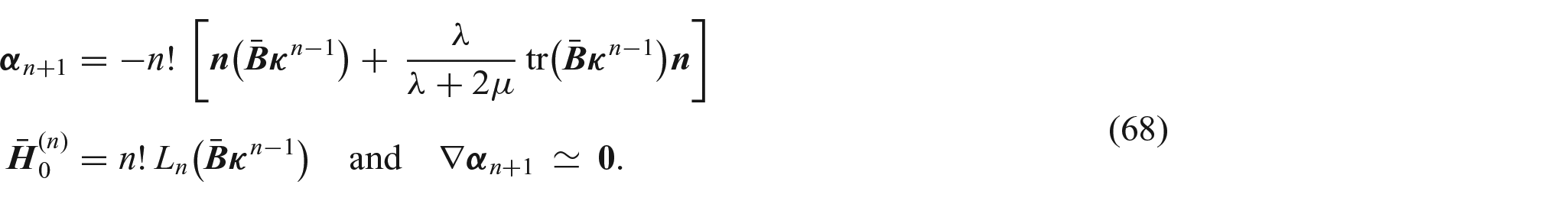
and by virtue of Lemma 1 and equation (69), we derive

$${\mathit{\alpha }}_{m+2}=-(m+1)![\mathit{n}(\overline{\mathit{B}}{\mathit{\kappa }}^m)+\frac{\lambda }{\lambda +2\mu }\mathrm{tr}(\overline{\mathit{B}}{\mathit{\kappa }}^m)\mathit{n}]\mathrm{and}{\overline{\mathit{H}}}_0^{(m+1)}=(m+1)!L_n(\overline{\mathit{B}}{\mathit{\kappa }}^m).$$

(71)

If we take the gradient of relation (71)₁ and then neglect the gradients of $\overline{\mathit{B}}$ as mentioned above, we deduce the approximation

$$\nabla {\mathit{\alpha }}_{m+2}\simeq 0.$$

(72)

Equations (71) and (72) show that relations (68) hold also for the order $n=m+1$ , so relations (68) are proved for any $n\ge 1$ by the induction procedure.

Taking into account definition (50), we see that relations (68) infer

$${\overline{\mathit{H}}}_0^{(n)}=n!\overline{\mathit{B}}{\mathit{\kappa }}^{n-1}+{\mathit{\alpha }}_{n+1}\otimes \mathit{n}\mathrm{for}\mathrm{any}n\ge 1,$$

(73)

where we consider ${\mathit{\kappa }}^0=\mathbb{1}$ for convenience.

3.2.3. Reconstruction of power series expansions

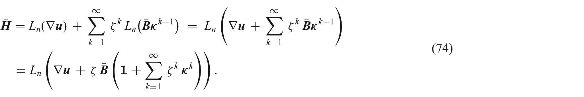
We can use now the power series expansion (37) to express the displacement gradient: from equations (54)₂, (58)₂, and (68)₂ we find

$$\begin{array}{c}\overline{\mathit{H}}=L_n(\nabla \mathit{u})+\sum _{k=1}^{\infty }{\zeta }^k{L}_n(\overline{\mathit{B}}{\mathit{\kappa }}^{k-1})=L_n(\nabla \mathit{u}+\sum _{k=1}^{\infty }{\zeta }^k\overline{\mathit{B}}{\mathit{\kappa }}^{k-1})\hfill \\ =L_n(\nabla \mathit{u}+\zeta \overline{\mathit{B}}(\mathbb{1}+\sum _{k=1}^{\infty }{\zeta }^k{\mathit{\kappa }}^k)).\hfill \end{array}$$

(74)

Furthermore, let us show the relation

$$\mathbb{1}+\sum _{k=1}^{\infty }{\zeta }^k{\mathit{\kappa }}^k={\mathit{\mu }}^{-1}.$$

(75)

Indeed, we have

$$\begin{array}{c}(1-2H\zeta +K{\zeta }^2)(\mathbb{1}+\sum _{k=1}^{\infty }{\zeta }^k{\mathit{\kappa }}^k)=(\mathbb{1}+\sum _{k=1}^{\infty }{\zeta }^k{\mathit{\kappa }}^k)-2H(\zeta \mathbb{1}+\sum _{k=1}^{\infty }{\zeta }^{k+1}{\mathit{\kappa }}^k)+K({\zeta }^2\mathbb{1}+\sum _{k=1}^{\infty }{\zeta }^{k+2}{\mathit{\kappa }}^k)\hfill \\ \multicolumn{1}{c}{=\mathbb{1}+\zeta \mathit{\kappa }-2H\zeta \mathbb{1}+\sum _{n=2}^{\infty }{\zeta }^n({\mathit{\kappa }}^n-2H{\mathit{\kappa }}^{n-1}+K{\mathit{\kappa }}^{n-2})}\\ \multicolumn{1}{c}{=\mathbb{1}+\zeta (\mathit{\kappa }-2H\mathbb{1}),}\end{array}$$

since ${\mathit{\kappa }}^n-2H{\mathit{\kappa }}^{n-1}+K{\mathit{\kappa }}^{n-2}=({\mathit{\kappa }}^2-2H\mathit{\kappa }+K\mathbb{1}){\mathit{\kappa }}^{n-2}=0$ , in view of equation (4). Then, we divide the above relation by $b(\zeta )$ and we deduce

$$\mathbb{1}+\sum _{k=1}^{\infty }{\zeta }^k{\mathit{\kappa }}^k=\frac{1}{b(\zeta )}(\mathbb{1}-\zeta {\mathit{\kappa }}^{*})={\mathit{\mu }}^{-1},$$

i.e., relation (75) holds. Substituting equation (75) into equation (74), we finally obtain the displacement gradient in the form

$$\overline{\mathit{H}}=L_n(\nabla \mathit{u}+\zeta \overline{\mathit{B}}{\mathit{\mu }}^{-1}).$$

(76)

Remark: We can alternatively justify the last relation in the following way: by virtue of the power series expansion of $\hat{\mathit{u}}$ given by relation (35), the displacement gradient can be represented as

$$\nabla \hat{\mathit{u}}=\nabla \mathit{u}+\zeta \nabla \mathit{a}+\sum _{k=2}^{\infty }\frac{1}{k!}{\zeta }^k\nabla {\mathit{\alpha }}_k.$$

Hence, the adoption of the approximations $\nabla {\mathit{\alpha }}_k\simeq 0$ (for $k\ge 2$ , cf. equation (68)) is tantamount to assume the approximation

$$\nabla \hat{\mathit{u}}\simeq \nabla \mathit{u}+\zeta \nabla \overline{\mathit{a}},$$

(77)

where $\overline{\mathit{a}}$ is given by equation (54) (i.e., $\overline{\mathit{a}}$ is obtained from the equation ${\mathit{P}}_0\mathit{n}=0$ ).

On the basis of equations (77) and (38), we can express the three-dimensional displacement gradient as follows

$$\overline{\mathit{H}}=(\nabla \mathit{u}+\zeta \nabla \overline{\mathit{a}}){\mathit{\mu }}^{-1}+{\hat{\mathit{u}}}^{\prime }\otimes \mathit{n}$$

and substituting here the relation

$$\nabla \mathit{u}=(\nabla \mathit{u})\mathbb{1}=(\nabla \mathit{u})(\mathit{\mu }+\zeta \mathit{\kappa })=(\nabla \mathit{u})\mathit{\mu }+\zeta (\nabla \mathit{u})\mathit{\kappa },$$

we find

$$\overline{\mathit{H}}=\nabla \mathit{u}+\zeta [(\nabla \mathit{u})\mathit{\kappa }+\nabla \overline{\mathit{a}}]{\mathit{\mu }}^{-1}+{\hat{\mathit{u}}}^{\prime }\otimes \mathit{n}=(\nabla \mathit{u}+\zeta \overline{\mathit{B}}{\mathit{\mu }}^{-1})+{\hat{\mathit{u}}}^{\prime }\otimes \mathit{n},$$

(78)

so we have

$$\overline{\mathit{H}}\mathbb{1}=\nabla \mathit{u}+\zeta \overline{\mathit{B}}{\mathit{\mu }}^{-1},$$

(79)

where $\overline{\mathit{B}}$ is given by equation (57) (or equation (59)).

On the other hand, in view of the power series expansion about $\zeta =0$

$$\mathit{Pn}={\mathit{P}}_0\mathit{n}+\sum _{k=1}^{\infty }\frac{1}{k!}{\zeta }^k{\mathit{P}}_0^{(k)}\mathit{n},$$

we see that the approximations ${\mathit{P}}_0^{(k)}\mathit{n}\simeq 0$ (for $k\ge 0$ , cf. equation (45)) are tantamount to assume the approximation (for small thickness $h$ )

$$\mathit{Pn}\simeq 0.$$

(80)

If we write the last relation in the form of the equation $\mathit{P}(\overline{\mathit{H}})\mathit{n}=0$ , then from Lemma 1 we deduce

$$\overline{\mathit{H}}=L_n(\overline{\mathit{H}}\mathbb{1}),$$

and using equation (79) we obtain

$$\overline{\mathit{H}}=L_n(\nabla \mathit{u}+\zeta \overline{\mathit{B}}{\mathit{\mu }}^{-1}),$$

which confirms the result (76) that was derived previously by means of power series expansions.

3.3. Integration over the thickness

We proceed to determine the expression of the areal strain energy density by computing the integral in equation (34). To this aim, we employ the displacement gradient $\overline{\mathit{H}}$ given by equation (76) and the following auxiliary result.

Lemma 2. Consider the bilinear forms $W_s(·,·)$ and $W_{3\mathrm{d}}(·,·)$ defined by equations (24), (30) and the linear operator $L_n$ defined by equation (50). Then, for any tensors $\mathit{X}=X_{i\alpha }{\mathit{a}}^i\otimes {\mathit{a}}^{\alpha }$ , $\mathit{Y}=Y_{i\alpha }{\mathit{a}}^i\otimes {\mathit{a}}^{\alpha }$ the following relations hold:

• $W_{3\mathrm{d}}(\mathit{X},\mathit{Y})=W_s(\mathit{X},\mathit{Y})+\frac{{\lambda }^2}{2(\lambda +2\mu )}(\mathrm{tr}\mathit{X})(\mathrm{tr}\mathit{Y})+\frac{\mu }{2}(\mathit{nX})(\mathit{nY}),$

• $W_{3\mathrm{d}}(L_n(\mathit{X}),\mathit{Y})=W_s(\mathit{X},\mathit{Y}),$

• $W_s(\mathit{X},\mathit{Y})=W_s(\mathbb{1}\mathit{X},\mathit{Y})=W_s(\mathrm{sym}(\mathbb{1}\mathit{X}),\mathit{Y}).$

Proof. (i) In view of the decomposition $\mathit{X}=\mathbb{1}\mathit{X}+\mathit{n}\otimes \mathit{nX}$ , it is clear that

$$\mathrm{sym}(\mathit{X})·\mathrm{sym}(\mathit{Y})=\mathrm{sym}(\mathbb{1}\mathit{X})·\mathrm{sym}(\mathbb{1}\mathit{Y})+\frac{1}{2}(\mathit{nX})·(\mathit{nY}).$$

Using this equation and the relation

$$\frac{\lambda }{2}=\frac{\lambda \mu }{\lambda +2\mu }+\frac{{\lambda }^2}{2(\lambda +2\mu )}$$

we obtain the desired result (i).

(ii) Let us denote for the moment by $\mathit{w}$ the vector $\mathit{w}:=\mathit{nX}+\frac{\lambda }{\lambda +2\mu }(\mathrm{tr}\mathit{X})\mathit{n}$ . Then, we have $L_n(\mathit{X})=\mathit{X}-\mathit{w}\otimes \mathit{n}$ , so it follows

$$W_{3\mathrm{d}}(L_n(\mathit{X}),\mathit{Y})=W_{3\mathrm{d}}(\mathit{X},\mathit{Y})-W_{3\mathrm{d}}(\mathit{w}\otimes \mathit{n},\mathit{Y}).$$

(81)

By a straightforward calculation based on the definition (30), we find that

$$W_{3\mathrm{d}}(\mathit{w}\otimes \mathit{n},\mathit{Y})=\frac{{\lambda }^2}{2(\lambda +2\mu )}(\mathrm{tr}\mathit{X})(\mathrm{tr}\mathit{Y})+\frac{\mu }{2}(\mathit{nX})(\mathit{nY}).$$

(82)

Inserting equation (82) into equation (81) and taking into account relation (i), we obtain

$$W_{3\mathrm{d}}(L_n(\mathit{X}),\mathit{Y})=W_{3\mathrm{d}}(\mathit{X},\mathit{Y})-\frac{{\lambda }^2}{2(\lambda +2\mu )}(\mathrm{tr}\mathit{X})(\mathrm{tr}\mathit{Y})-\frac{\mu }{2}(\mathit{nX})(\mathit{nY})=W_s(\mathit{X},\mathit{Y}),$$

i.e., relation (ii) is proved.

(iii) Since $\mathrm{tr}\mathit{X}=\mathrm{tr}(\mathbb{1}\mathit{X})=\mathrm{tr}\mathrm{sym}(\mathbb{1}\mathit{X})$ , we derive directly from definition (24) that relations (iii) hold true. ■

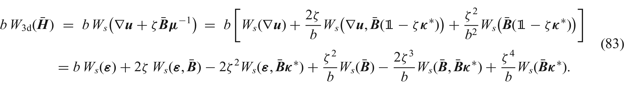
By virtue of Lemma 2 and relations (6) and (76), we can transform the integrand in equation (34) as follows:

$$\begin{array}{c}b{W}_{3\mathrm{d}}(\overline{\mathit{H}})=b{W}_s(\nabla \mathit{u}+\zeta \overline{\mathit{B}}{\mathit{\mu }}^{-1})=b[W_s(\nabla \mathit{u})+\frac{2\zeta }{b}{W}_s(\nabla \mathit{u},\overline{\mathit{B}}(\mathbb{1}-\zeta {\mathit{\kappa }}^{*}))+\frac{{\zeta }^2}{b^2}{W}_s(\overline{\mathit{B}}(\mathbb{1}-\zeta {\mathit{\kappa }}^{*}))]\hfill \\ \multicolumn{1}{c}{=b{W}_s(\mathit{\epsilon })+2\zeta W_s(\mathit{\epsilon },\overline{\mathit{B}})-2{\zeta }^2{W}_s(\mathit{\epsilon },\overline{\mathit{B}}{\mathit{\kappa }}^{*})+\frac{{\zeta }^2}{b}{W}_s(\overline{\mathit{B}})-\frac{2{\zeta }^3}{b}{W}_s(\overline{\mathit{B}},\overline{\mathit{B}}{\mathit{\kappa }}^{*})+\frac{{\zeta }^4}{b}{W}_s(\overline{\mathit{B}}{\mathit{\kappa }}^{*}).}\end{array}$$

(83)

We insert equation (83) into equation (34) and integrate over the thickness to find the following form of the areal strain energy density:

$${\overline{\mathcal{W}}}_{\mathrm{shell}}(\mathit{\epsilon },\mathit{\rho })=(h+K\frac{h^3}{12})W_s(\mathit{\epsilon })-2\frac{h^3}{12}{W}_s(\mathit{\epsilon },\overline{\mathit{B}}{\mathit{\kappa }}^{*})+J_2{W}_s(\overline{\mathit{B}})-2J_3{W}_s(\overline{\mathit{B}},\overline{\mathit{B}}{\mathit{\kappa }}^{*})+J_4{W}_s(\overline{\mathit{B}}{\mathit{\kappa }}^{*}),$$

(84)

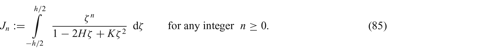
where $\overline{\mathit{B}}$ is given by equation (59) and we denote by $J_n$ the integrals

$$J_n:=\underset{-h/2}{\overset{h/2}{\int }}\frac{{\zeta }^n}{1-2H\zeta +K{\zeta }^2}\mathrm{d}\zeta \mathrm{for}\mathrm{any}\mathrm{integer}n\ge 0.$$

(85)

3.3.1. Explicit form of the coefficients in the strain energy density

Note that the coefficients appearing in the areal strain energy density (84) depend on the curvature of the reference midsurface and they involve the integrals $J_k$ of type (85) with $k\in \{2,3,4\}$ . Next, we want to determine the explicit form of the integrals $J_k$ .

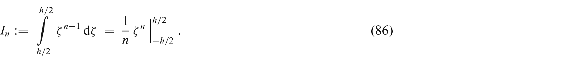
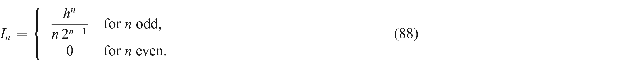
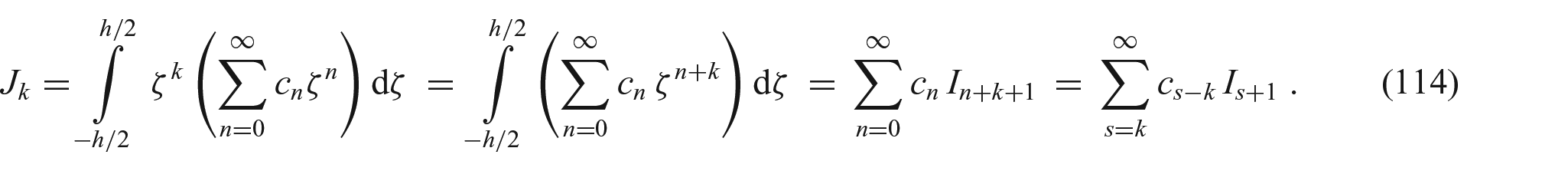
To this aim, let us denote by $(I_n{)}_{n\ge 1}$ the sequence of integrals

$$I_n:=\underset{-h/2}{\overset{h/2}{\int }}{\zeta }^{n-1}\mathrm{d}\zeta =\frac{1}{n}{\zeta }^n{|}_{-h/2}^{h/2}.$$

(86)

We see that

$$I_1=h,I_3=\frac{h^3}{12},I_5=\frac{h^5}{80},I_7=\frac{h^7}{448},\dots$$

(87)

and we have in general

$$I_n=\{\begin{array}{cc}\frac{h^n}{n{2}^{n-1}}\hfill & \mathrm{for}n\mathrm{odd},\hfill \\ \multicolumn{1}{c}{0}& \mathrm{for}n\mathrm{even}.\hfill \end{array}$$

(88)

Using this notation, we can write for the integrals $J_n$ the following recurrence relation

$$J_n=\frac{1}{K}(I_{n-1}+2H{J}_{n-1}-J_{n-2})\mathrm{for}\mathrm{any}n\ge 2,$$

(89)

which can be justified by a simple transformation of the integral in equation (85).

In what follows, we need to expand the function $\frac{1}{b(\zeta )}$ as a power series of $\zeta$ . In this respect, we prove the useful result:

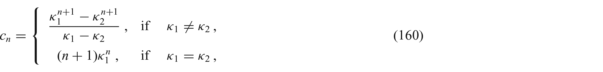
Lemma 3. Denote by $(c_n{)}_{n\ge 0}$ the sequence of coefficients in the power series expansion

$$\frac{1}{1-2H\zeta +K{\zeta }^2}=c_0+c_1\zeta +c_2{\zeta }^2+\cdots +c_n{\zeta }^n+\cdots =\sum _{n=0}^{\infty }{c}_n{\zeta }^n.$$

(90)

Then, the sequence $(c_n{)}_{n\ge 0}$ satisfies the recursive equation

$$c_0=1,c_1=2H\mathrm{and}{c}_{n+1}=2H{c}_n-K{c}_{n-1}\mathrm{for}\mathrm{any}n\ge 1.$$

(91)

Moreover, the coefficients $c_n$ can be written as polynomial functions of the mean curvature $H$ and the Gauss curvature $K$ in the following explicit form:

$$c_n=\sum _{i=0}^{[n/2]}(-1{)}^i\left(\begin{array}{c}n-i\hfill \\ \multicolumn{1}{c}{i}\end{array}\right)(2H{)}^{n-2i}{K}^i,$$

(92)

where $[n/2]$ designates the biggest integer number not exceeding $n/2$ .

Proof. Let ${\kappa }_1$ and ${\kappa }_2$ denote the principal curvatures of the reference midsurface $\mathrm{\Omega }$ and $R_{\alpha }=|{\kappa }_{\alpha }{|}^{-1}$ the radii of curvature. Then, we have

$${\kappa }_1+{\kappa }_2=2H,{\kappa }_1{\kappa }_2=K$$

(93)

and it follows

$$b(\zeta )=1-2H\zeta +K{\zeta }^2=(1-{\kappa }_1\zeta )(1-{\kappa }_2\zeta )>0,$$

(94)

since $\zeta \in (\frac{h}{2},-\frac{h}{2})$ and we assume for thin shells that

$$h<<R_1,h<<R_2.$$

Thus, we have $|{\kappa }_{\alpha }\zeta |<<1$ , so we can write the power series expansion

$$\frac{1}{1-{\kappa }_{\alpha }\zeta }=1+{\kappa }_{\alpha }\zeta +({\kappa }_{\alpha }\zeta {)}^2+\cdots +({\kappa }_{\alpha }\zeta {)}^n+\cdots =\sum _{n=0}^{\infty }({\kappa }_{\alpha }\zeta {)}^n\mathrm{for}\alpha =1,2.$$

(95)

Then, we consider the Cauchy product of the two power series in equation (95) and obtain

$$\frac{1}{(1-{\kappa }_1\zeta )(1-{\kappa }_2\zeta )}=\left(\sum _{n=0}^{\infty }{\kappa }_1^n{\zeta }^n\right)\left(\sum _{m=0}^{\infty }{\kappa }_2^m{\zeta }^m\right),$$

i.e.,

$$\frac{1}{1-2H\zeta +K{\zeta }^2}=\sum _{n=0}^{\infty }({\kappa }_1^n+{\kappa }_1^{n-1}{\kappa }_2+\cdots +{\kappa }_1{\kappa }_2^{n-1}+{\kappa }_2^n){\zeta }^n.$$

(96)

By comparing equations (90) and (96), we get

$$c_n={\kappa }_1^n+{\kappa }_1^{n-1}{\kappa }_2+\cdots +{\kappa }_1{\kappa }_2^{n-1}+{\kappa }_2^n=\sum _{i=0}^n{\kappa }_1^{n-i}{\kappa }_2^i.$$

(97)

On the basis of equation (97), we can show now the recursive relation (91). Indeed, we have $c_0=1$ , $c_1={\kappa }_1+{\kappa }_2=2H$ and

$$\begin{array}{c}2H{c}_n-K{c}_{n-1}=({\kappa }_1+{\kappa }_2)({\kappa }_1^n+{\kappa }_1^{n-1}{\kappa }_2+\cdots +{\kappa }_1{\kappa }_2^{n-1}+{\kappa }_2^n)\hfill \\ \multicolumn{1}{c}{-({\kappa }_1{\kappa }_2)({\kappa }_1^{n-1}+{\kappa }_1^{n-2}{\kappa }_2+\cdots +{\kappa }_1{\kappa }_2^{n-2}+{\kappa }_2^{n-1})}\\ \multicolumn{1}{c}{={\kappa }_1^{n+1}+{\kappa }_1^n{\kappa }_2+\cdots +{\kappa }_1{\kappa }_2^n+{\kappa }_2^{n+1}=c_{n+1}}\end{array}$$

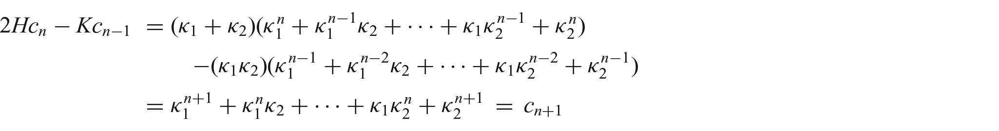
and relation (91) is proved. To verify the formula (92), we employ the general polynomial identity

$$x^n+x^{n-1}y+\cdots +x{y}^{n-1}+y^n=\sum _{k=0}^{[n/2]}(-1{)}^k\left(\begin{array}{c}n-k\hfill \\ \multicolumn{1}{c}{k}\end{array}\right)(x+y{)}^{n-2k}(\mathrm{xy}{)}^k,$$

(98)

which holds for any $x,y\in \mathbb{R}$ . This identity can be proved by mathematical induction with respect to $n$ (see a proof in Appendix). If we apply relation (98) for $x={\kappa }_1$ , $y={\kappa }_2$ and take into account (97), then we obtain

$$c_n=\sum _{k=0}^{[n/2]}(-1{)}^k\left(\begin{array}{c}n-k\hfill \\ \multicolumn{1}{c}{k}\end{array}\right)({\kappa }_1+{\kappa }_2{)}^{n-2k}({\kappa }_1{\kappa }_2{)}^k$$

and in view of equation (93), we see that relation (92) holds true. ■

From the recurrence relation (91), we can easily compute the first coefficients in the expansion (90) as follows:

$$c_0=1,c_1=2H,c_2=4H^2-K,c_3=8H^3-4\mathrm{HK},c_4=16H^4-12H^{2}K+K^2,\mathrm{etc}.$$

(99)

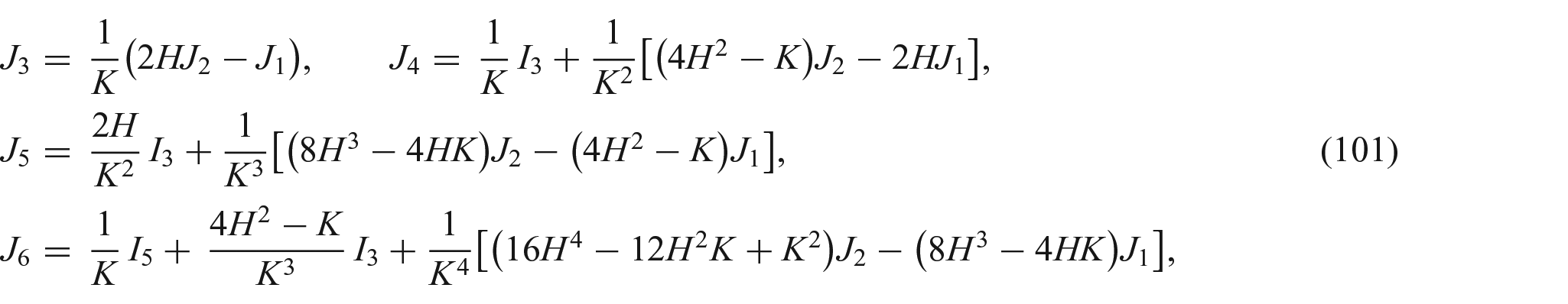
Using Lemma 3 and the recurrence relation (89), we can prove by induction that the following equation holds:

$$J_n=\left(\sum _{s=1}^{n-2}\frac{c_{s-1}}{K^s}{I}_{n-s}\right)+\frac{1}{K^{n-2}}(c_{n-2}{J}_2-c_{n-3}{J}_1)\mathrm{for}\mathrm{any}n\ge 3.$$

(100)

Hence, for $n\in \{3,4,5,6\}$ , we obtain the relations

$$\begin{array}{c}{J}_3=\frac{1}{K}(2H{J}_2-J_1),J_4=\frac{1}{K}{I}_3+\frac{1}{K^2}[(4H^2-K)J_2-2H{J}_1],\hfill \\ \multicolumn{1}{c}{J_5=\frac{2H}{K^2}{I}_3+\frac{1}{K^3}[(8H^3-4\mathrm{HK})J_2-(4H^2-K)J_1],}\\ \multicolumn{1}{c}{J_6=\frac{1}{K}{I}_5+\frac{4H^2-K}{K^3}{I}_3+\frac{1}{K^4}[(16H^4-12H^{2}K+K^2)J_2-(8H^3-4\mathrm{HK})J_1],}\end{array}$$

(101)

where we have used equation (99). Inserting $J_3$ and $J_4$ from equation (101) into equation (84), we find the following expressions of the strain energy density:

$$\begin{array}{c}{\overline{\mathcal{W}}}_{\mathrm{shell}}(\mathit{\epsilon },\mathit{\rho })=(h+K\frac{h^3}{12})W_s(\mathit{\epsilon })-2\frac{h^3}{12}{W}_s(\mathit{\epsilon },\overline{\mathit{B}}{\mathit{\kappa }}^{*})+J_2{W}_s(\overline{\mathit{B}})\hfill \\ \multicolumn{1}{c}{-\frac{2}{K}(2H{J}_2-J_1)W_s(\overline{\mathit{B}},\overline{\mathit{B}}{\mathit{\kappa }}^{*})+\frac{1}{K}[\frac{h^3}{12}+(\frac{4H^2}{K}-1)J_2-\frac{2H}{K}{J}_1]W_s(\overline{\mathit{B}}{\mathit{\kappa }}^{*}).}\end{array}$$

(102)

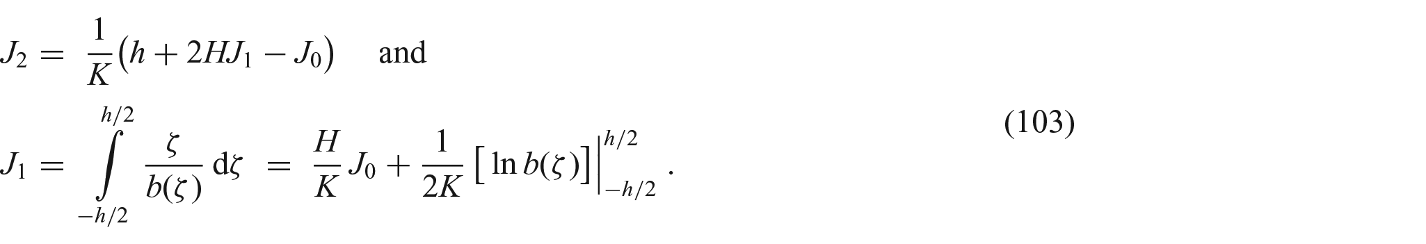
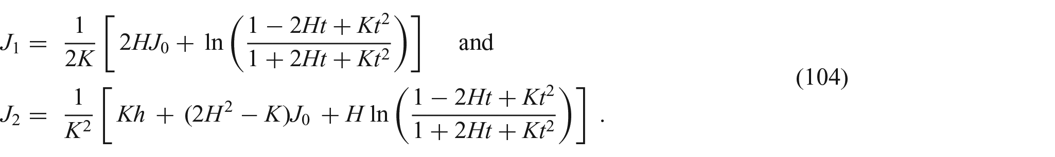
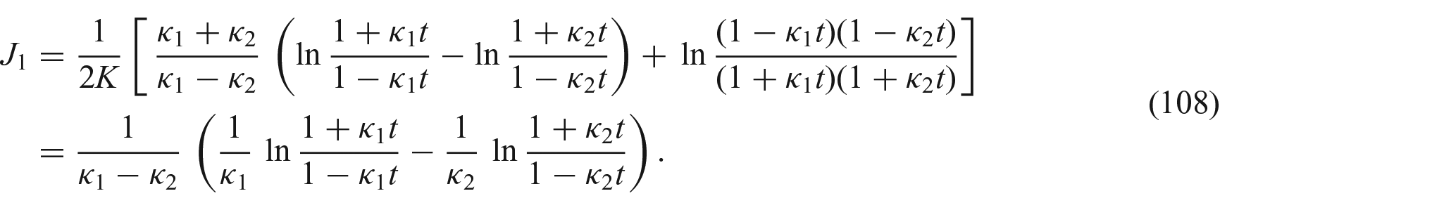
It remains to determine the integrals $J_1$ and $J_2$ which appear in the above coefficients of relation (102). We remark that $J_1$ and $J_2$ can be expressed in terms of $J_0$ . Indeed, in view of equations (85) and (89), we have

$$\begin{array}{c}{J}_2=\frac{1}{K}(h+2H{J}_1-J_0)\mathrm{and}\hfill \\ \multicolumn{1}{c}{J_1=\underset{-h/2}{\overset{h/2}{\int }}\frac{\zeta }{b(\zeta )}\mathrm{d}\zeta =\frac{H}{K}{J}_0+\frac{1}{2K}[\ln b(\zeta )]{|}_{-h/2}^{h/2}.}\end{array}$$

(103)

For convenience, let us denote for the moment the shell thickness with $2t$ , i.e., $t:=h/2$ . Thus, we obtain

$$\begin{array}{c}{J}_1=\frac{1}{2K}[2H{J}_0+\ln \left(\frac{1-2\mathrm{Ht}+K{t}^2}{1+2\mathrm{Ht}+K{t}^2}\right)]\mathrm{and}\hfill \\ \multicolumn{1}{c}{J_2=\frac{1}{K^2}[\mathrm{Kh}+(2H^2-K)J_0+H\ln \left(\frac{1-2\mathrm{Ht}+K{t}^2}{1+2\mathrm{Ht}+K{t}^2}\right)].}\end{array}$$

(104)

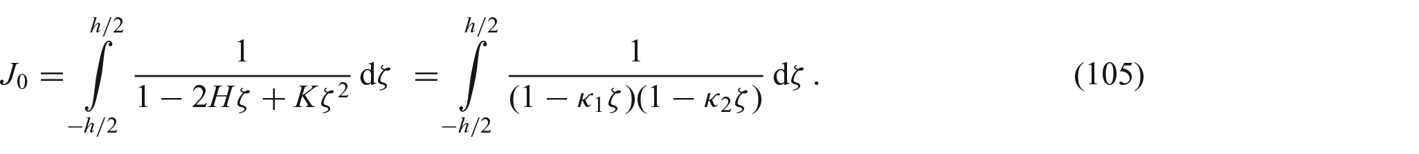
Now we only need to compute the integral $J_0$ , which can be written as

$$J_0=\underset{-h/2}{\overset{h/2}{\int }}\frac{1}{1-2H\zeta +K{\zeta }^2}\mathrm{d}\zeta =\underset{-h/2}{\overset{h/2}{\int }}\frac{1}{(1-{\kappa }_1\zeta )(1-{\kappa }_2\zeta )}\mathrm{d}\zeta .$$

(105)

In the case ${\kappa }_1\ne {\kappa }_2$ , we obtain

$$J_0=\frac{1}{{\kappa }_1-{\kappa }_2}\ln \left(\frac{1+({\kappa }_1-{\kappa }_2)t-K{t}^2}{1-({\kappa }_1-{\kappa }_2)t-K{t}^2}\right),$$

(106)

or equivalently,

$$J_0=\frac{1}{{\kappa }_1-{\kappa }_2}(\ln \frac{1+{\kappa }_{1}t}{1-{\kappa }_{1}t}-\ln \frac{1+{\kappa }_{2}t}{1-{\kappa }_{2}t}).$$

(107)

Then, from equations (104) and (107) we get

$$\begin{array}{c}{J}_1=\frac{1}{2K}[\frac{{\kappa }_1+{\kappa }_2}{{\kappa }_1-{\kappa }_2}(\ln \frac{1+{\kappa }_{1}t}{1-{\kappa }_{1}t}-\ln \frac{1+{\kappa }_{2}t}{1-{\kappa }_{2}t})+\ln \frac{(1-{\kappa }_{1}t)(1-{\kappa }_{2}t)}{(1+{\kappa }_{1}t)(1+{\kappa }_{2}t)}]\hfill \\ \multicolumn{1}{c}{=\frac{1}{{\kappa }_1-{\kappa }_2}(\frac{1}{{\kappa }_1}\ln \frac{1+{\kappa }_{1}t}{1-{\kappa }_{1}t}-\frac{1}{{\kappa }_2}\ln \frac{1+{\kappa }_{2}t}{1-{\kappa }_{2}t}).}\end{array}$$

(108)

For $n\ge 2$ we can show the general formula

$$J_n=\left(\sum _{s=1}^{n-1}\frac{c_{s-1}}{K^s}{I}_{n-s}\right)+\frac{1}{{\kappa }_1-{\kappa }_2}(\frac{1}{{\kappa }_1^n}\ln \frac{1+{\kappa }_{1}t}{1-{\kappa }_{1}t}-\frac{1}{{\kappa }_2^n}\ln \frac{1+{\kappa }_{2}t}{1-{\kappa }_{2}t}).$$

(109)

Indeed, to prove the last relation we start from the equality

$$c_{n-2}{J}_2-c_{n-3}{J}_1=\frac{1}{K}(c_{n-2}h+c_{n-1}{J}_1-c_{n-2}{J}_0),$$

(110)

which follows from the recurrence equation (91). Inserting the last relation in equation (100) we deduce

$$J_n=\left(\sum _{s=1}^{n-1}\frac{c_{s-1}}{K^s}{I}_{n-s}\right)+\frac{1}{K^{n-1}}(c_{n-1}{J}_1-c_{n-2}{J}_0)\mathrm{for}\mathrm{any}n\ge 2.$$

(111)

Furthermore, in view of equation (97) we have

$$c_{n-1}{J}_1-c_{n-2}{J}_0=\frac{{\kappa }_1^n-{\kappa }_2^n}{{\kappa }_1-{\kappa }_2}{J}_1-\frac{{\kappa }_1^{n-1}-{\kappa }_2^{n-1}}{{\kappa }_1-{\kappa }_2}{J}_0$$

and substituting here equations (107) and (108) we derive

$$c_{n-1}{J}_1-c_{n-2}{J}_0=\frac{{({\kappa }_1{\kappa }_2)}^{n-1}}{{\kappa }_1-{\kappa }_2}(\frac{1}{{\kappa }_1^n}\ln \frac{1+{\kappa }_{1}t}{1-{\kappa }_{1}t}-\frac{1}{{\kappa }_2^n}\ln \frac{1+{\kappa }_{2}t}{1-{\kappa }_{2}t}).$$

(112)

Finally, using equation (112) in equation (111), we see that the general relation (109) holds true.

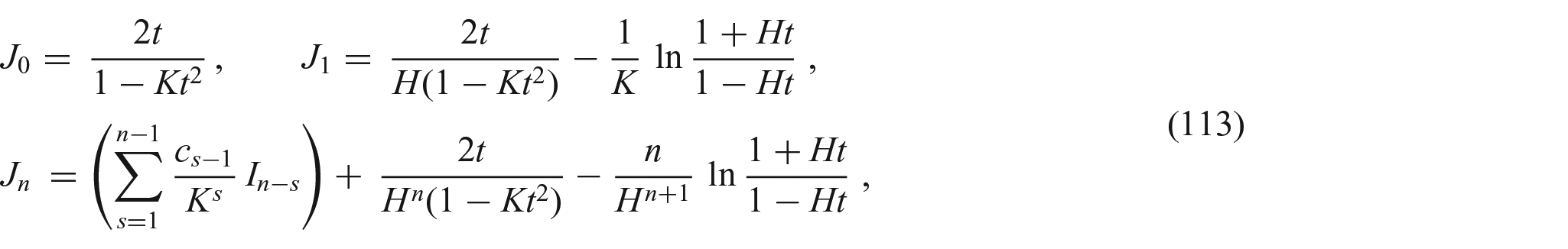
In the case ${\kappa }_1={\kappa }_2$ (umbilic point), we can extend relations (107), (108), and (109) by continuity and obtain

$$\begin{array}{c}{J}_0=\frac{2t}{1-K{t}^2},J_1=\frac{2t}{H(1-K{t}^2)}-\frac{1}{K}\ln \frac{1+\mathrm{Ht}}{1-\mathrm{Ht}},\hfill \\ \multicolumn{1}{c}{J_n=\left(\sum _{s=1}^{n-1}\frac{c_{s-1}}{K^s}{I}_{n-s}\right)+\frac{2t}{H^n(1-K{t}^2)}-\frac{n}{H^{n+1}}\ln \frac{1+\mathrm{Ht}}{1-\mathrm{Ht}},}\end{array}$$

(113)

with $H={\kappa }_1={\kappa }_2$ and $K={\kappa }_1{\kappa }_2=H^2$ .

In conclusion, relations (107)–(109) and (113) give the explicit expressions of integrals $J_n$ appearing in the constitutive coefficients, in terms of $H$ , $K$ and the principal curvatures ${\kappa }_1,{\kappa }_2$ of the reference midsurface. The obtained form of the areal strain energy density ${\overline{\mathcal{W}}}_{\mathrm{shell}}(\mathit{\epsilon },\mathit{\rho })$ is given by relation (84).

3.4. The shell model of order $O(h^n)$

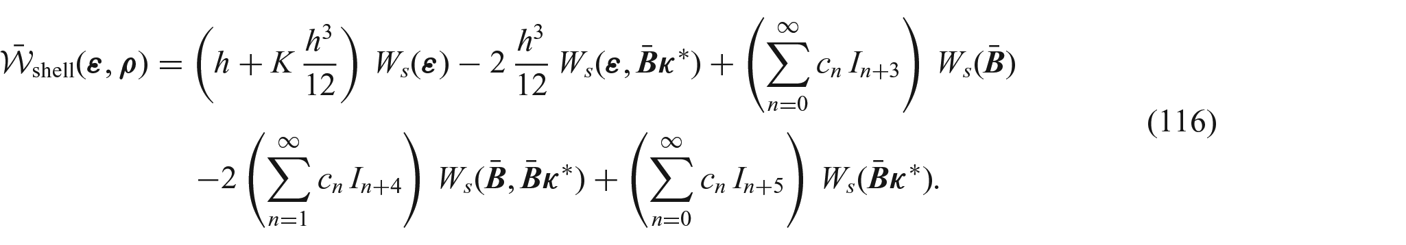
Let us represent the strain energy density (84) in an alternative form by expanding the coefficients $J_2,J_3$ , and $J_4$ as power series of $h$ .

In view of Lemma 3 and definition (85), we have

$$J_k=\underset{-h/2}{\overset{h/2}{\int }}{\zeta }^k\left(\sum _{n=0}^{\infty }{c}_n{\zeta }^n\right)\mathrm{d}\zeta =\underset{-h/2}{\overset{h/2}{\int }}\left(\sum _{n=0}^{\infty }{c}_n{\zeta }^{n+k}\right)\mathrm{d}\zeta =\sum _{n=0}^{\infty }{c}_n{I}_{n+k+1}=\sum _{s=k}^{\infty }{c}_{s-k}{I}_{s+1}.$$

(114)

Taking into account that $I_{2r}=0$ for any $r\ge 1$ , the last relation can also be written in the form

$$J_k=\sum _{r=[\frac{k+1}{2}]}^{\infty }{c}_{2r-k}{I}_{2r+1}.$$

(115)

Using relations of this type for $J_2,J_3,J_4$ in equation (84), we obtain the following alternative expression of the strain energy density

$$\begin{array}{c}{\overline{\mathcal{W}}}_{\mathrm{shell}}(\mathit{\epsilon },\mathit{\rho })=(h+K\frac{h^3}{12})W_s(\mathit{\epsilon })-2\frac{h^3}{12}{W}_s(\mathit{\epsilon },\overline{\mathit{B}}{\mathit{\kappa }}^{*})+\left(\sum _{n=0}^{\infty }{c}_n{I}_{n+3}\right)W_s(\overline{\mathit{B}})\hfill \\ \multicolumn{1}{c}{-2\left(\sum _{n=1}^{\infty }{c}_n{I}_{n+4}\right)W_s(\overline{\mathit{B}},\overline{\mathit{B}}{\mathit{\kappa }}^{*})+\left(\sum _{n=0}^{\infty }{c}_n{I}_{n+5}\right)W_s(\overline{\mathit{B}}{\mathit{\kappa }}^{*}).}\end{array}$$

(116)

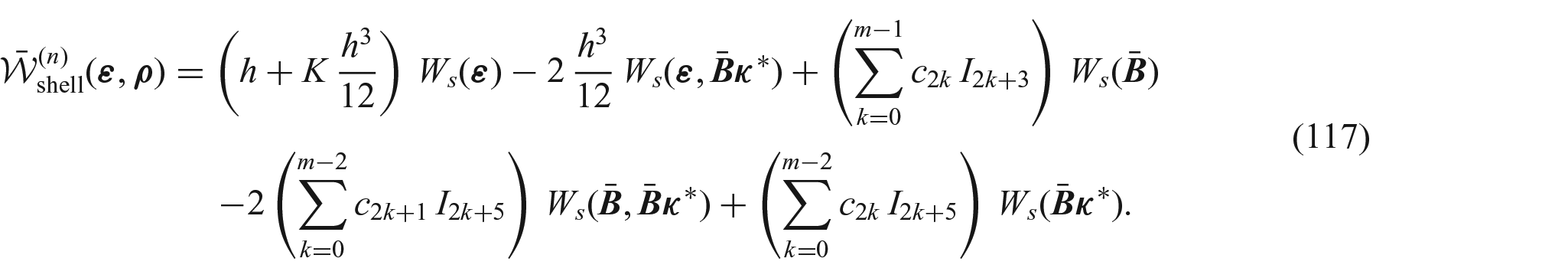
To derive now a shell model of order $O(h^n)$ with $n=2m+1$ , we truncate the power series appearing in the coefficients of equation (116) by retaining only the terms up to $h^n$ . Thus, we obtain the following strain energy density:

$$\begin{array}{c}{\overline{\mathcal{W}}}_{\mathrm{shell}}^{(n)}(\mathit{\epsilon },\mathit{\rho })=(h+K\frac{h^3}{12})W_s(\mathit{\epsilon })-2\frac{h^3}{12}{W}_s(\mathit{\epsilon },\overline{\mathit{B}}{\mathit{\kappa }}^{*})+\left(\sum _{k=0}^{m-1}{c}_{2k}{I}_{2k+3}\right)W_s(\overline{\mathit{B}})\hfill \\ \multicolumn{1}{c}{-2\left(\sum _{k=0}^{m-2}{c}_{2k+1}{I}_{2k+5}\right)W_s(\overline{\mathit{B}},\overline{\mathit{B}}{\mathit{\kappa }}^{*})+\left(\sum _{k=0}^{m-2}{c}_{2k}{I}_{2k+5}\right)W_s(\overline{\mathit{B}}{\mathit{\kappa }}^{*}).}\end{array}$$

(117)

Remark: We observe that the last two terms in equation (117) are defined only for $m\ge 2$ , i.e., $n\ge 5$ . In the special case $n=3$ , we obtain the following energy density for the model of order $O(h^3)$

$${\overline{\mathcal{W}}}_{\mathrm{shell}}^{(3)}(\mathit{\epsilon },\mathit{\rho })=(h+K\frac{h^3}{12})W_s(\mathit{\epsilon })-2\frac{h^3}{12}{W}_s(\mathit{\epsilon },\overline{\mathit{B}}{\mathit{\kappa }}^{*})+\frac{h^3}{12}{W}_s(\overline{\mathit{B}}),$$

(118)

which is in agreement with the corresponding representations in classical approaches of linear shell theory (see the work by Steigmann et al. [9]).

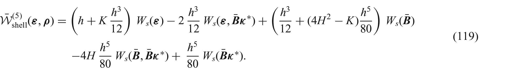
For $n=5$ , we obtain from equation (117) the strain energy density for the model of order $O(h^5)$ in the following form:

$$\begin{array}{c}{\overline{\mathcal{W}}}_{\mathrm{shell}}^{(5)}(\mathit{\epsilon },\mathit{\rho })=(h+K\frac{h^3}{12})W_s(\mathit{\epsilon })-2\frac{h^3}{12}{W}_s(\mathit{\epsilon },\overline{\mathit{B}}{\mathit{\kappa }}^{*})+(\frac{h^3}{12}+(4H^2-K)\frac{h^5}{80})W_s(\overline{\mathit{B}})\hfill \\ \multicolumn{1}{c}{-4H\frac{h^5}{80}{W}_s(\overline{\mathit{B}},\overline{\mathit{B}}{\mathit{\kappa }}^{*})+\frac{h^5}{80}{W}_s(\overline{\mathit{B}}{\mathit{\kappa }}^{*}).}\end{array}$$

(119)

Similarly, using the general expression (117), we can write down the strain energy densities for the shell models of order $O(h^7)$ , $O(h^9)$ , etc.

4. Simplification of the general shell model

We can obtain a simplified version of the general shell model provided we approximate the tensor $\overline{\mathit{B}}$ which appears in the expression of the strain energy density. Notice that the tensor $\overline{\mathit{B}}$ is given by relation (59).

During the derivation of the model in Section 3.2 we neglected the gradients of the strain measures $\mathit{\epsilon }$ , $\mathit{\rho }$ . Accordingly, it is consistent to neglect also the gradient $\nabla [(\mathrm{tr}\mathit{\epsilon })\mathit{n}]$ in relation (59), i.e., we approximate

$$\overline{\mathit{B}}\simeq -\mathit{\rho }+2\mathit{\epsilon }\mathit{\kappa }.$$

(120)

Thus, by replacing the tensor $\overline{\mathit{B}}$ with $(-\mathit{\rho }+2\mathit{\epsilon }\mathit{\kappa })$ in the expression of the strain energy density, we obtain a simplified version of the general shell model.

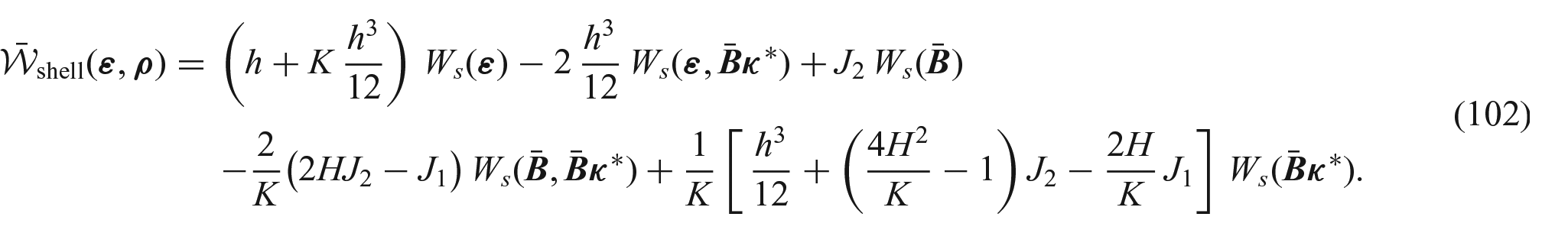
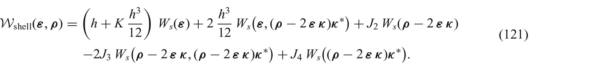
Let us write the new (simplified) forms of the strain energy density: substituting equation (120) in equation (84), we derive the compact form

$$\begin{array}{c}{\mathcal{W}}_{\mathrm{shell}}(\mathit{\epsilon },\mathit{\rho })=(h+K\frac{h^3}{12})W_s(\mathit{\epsilon })+2\frac{h^3}{12}{W}_s(\mathit{\epsilon },(\mathit{\rho }-2\mathit{\epsilon }\mathit{\kappa }){\mathit{\kappa }}^{*})+J_2{W}_s(\mathit{\rho }-2\mathit{\epsilon }\mathit{\kappa })\hfill \\ \multicolumn{1}{c}{-2J_3{W}_s(\mathit{\rho }-2\mathit{\epsilon }\mathit{\kappa },(\mathit{\rho }-2\mathit{\epsilon }\mathit{\kappa }){\mathit{\kappa }}^{*})+J_4{W}_s((\mathit{\rho }-2\mathit{\epsilon }\mathit{\kappa }){\mathit{\kappa }}^{*}).}\end{array}$$

(121)

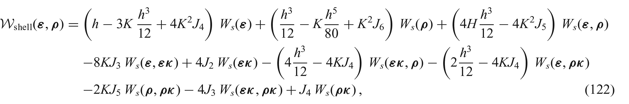
In the last relation, we can use the equation ${\mathit{\kappa }}^{*}=2H\mathbb{1}-\mathit{\kappa }$ , as well as $\mathit{\kappa }{\mathit{\kappa }}^{*}=K\mathbb{1}$ , to express the right-hand side in terms of the tensors $\mathit{\epsilon },\mathit{\rho },\mathit{\epsilon }\mathit{\kappa },$ and $\mathit{\rho }\mathit{\kappa }$ . Thus, by a straightforward calculation we can put equation (121) in the equivalent form

$$\begin{array}{c}{\mathcal{W}}_{\mathrm{shell}}(\mathit{\epsilon },\mathit{\rho })=(h-3K\frac{h^3}{12}+4K^2{J}_4)W_s(\mathit{\epsilon })+(\frac{h^3}{12}-K\frac{h^5}{80}+K^2{J}_6)W_s(\mathit{\rho })+(4H\frac{h^3}{12}-4K^2{J}_5)W_s(\mathit{\epsilon },\mathit{\rho })\hfill \\ -8K{J}_3{W}_s(\mathit{\epsilon },\mathit{\epsilon }\mathit{\kappa })+4J_2{W}_s(\mathit{\epsilon }\mathit{\kappa })-(4\frac{h^3}{12}-4K{J}_4)W_s(\mathit{\epsilon }\mathit{\kappa },\mathit{\rho })-(2\frac{h^3}{12}-4K{J}_4)W_s(\mathit{\epsilon },\mathit{\rho }\mathit{\kappa })\hfill \\ -2K{J}_5{W}_s(\mathit{\rho },\mathit{\rho }\mathit{\kappa })-4J_3{W}_s(\mathit{\epsilon }\mathit{\kappa },\mathit{\rho }\mathit{\kappa })+J_4{W}_s(\mathit{\rho }\mathit{\kappa }),\hfill \end{array}$$

(122)

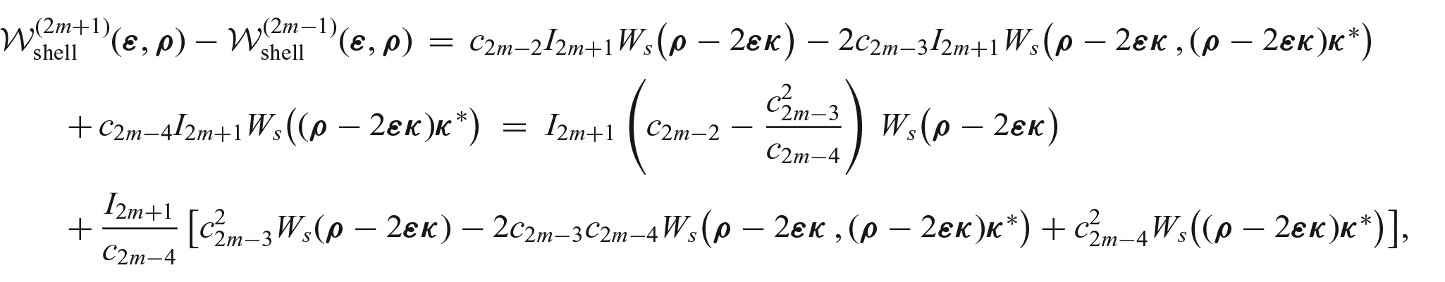
where we have also employed the recurrence relation (89) for $n\in \{4,5,6\}$ .

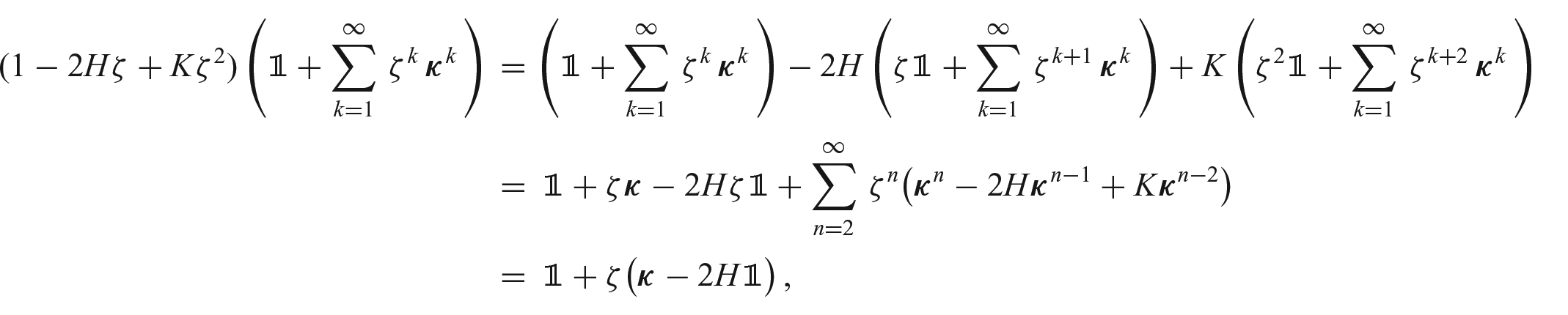
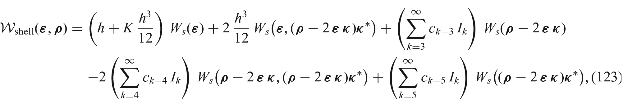
Notice that the coefficients in the above expressions (121), (122) can also be written with help of power series of $h$ . Thus, using expansions of the type (114), the strain energy density (121) can be written in the form

$$\begin{array}{c}{\mathcal{W}}_{\mathrm{shell}}(\mathit{\epsilon },\mathit{\rho })=(h+K\frac{h^3}{12})W_s(\mathit{\epsilon })+2\frac{h^3}{12}{W}_s(\mathit{\epsilon },(\mathit{\rho }-2\mathit{\epsilon }\mathit{\kappa }){\mathit{\kappa }}^{*})+\left(\sum _{k=3}^{\infty }{c}_{k-3}{I}_k\right)W_s(\mathit{\rho }-2\mathit{\epsilon }\mathit{\kappa })\hfill \\ -2\left(\sum _{k=4}^{\infty }{c}_{k-4}{I}_k\right)W_s(\mathit{\rho }-2\mathit{\epsilon }\mathit{\kappa },(\mathit{\rho }-2\mathit{\epsilon }\mathit{\kappa }){\mathit{\kappa }}^{*})+\left(\sum _{k=5}^{\infty }{c}_{k-5}{I}_k\right)W_s((\mathit{\rho }-2\mathit{\epsilon }\mathit{\kappa }){\mathit{\kappa }}^{*}),\hfill \end{array}$$

(123)

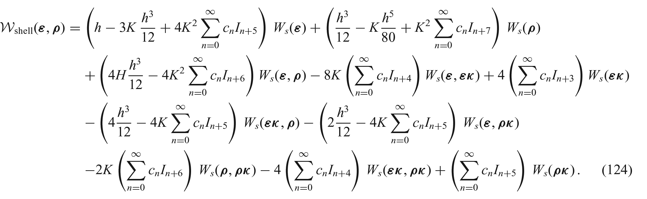
where all the $I_k$ with an even index are vanishing, i.e., $I_{2r}=0$ for all $r\ge 1$ . Similarly, the strain energy density (122) can be written alternatively by means of power series of $h$ as follows:

$$\begin{array}{c}{\mathcal{W}}_{\mathrm{shell}}(\mathit{\epsilon },\mathit{\rho })=(h-3K\frac{h^3}{12}+4K^2\sum _{n=0}^{\infty }{c}_n{I}_{n+5})W_s(\mathit{\epsilon })+(\frac{h^3}{12}-K\frac{h^5}{80}+K^2\sum _{n=0}^{\infty }{c}_n{I}_{n+7})W_s(\mathit{\rho })\hfill \\ +(4H\frac{h^3}{12}-4K^2\sum _{n=0}^{\infty }{c}_n{I}_{n+6})W_s(\mathit{\epsilon },\mathit{\rho })-8K\left(\sum _{n=0}^{\infty }{c}_n{I}_{n+4}\right)W_s(\mathit{\epsilon },\mathit{\epsilon }\mathit{\kappa })+4\left(\sum _{n=0}^{\infty }{c}_n{I}_{n+3}\right)W_s(\mathit{\epsilon }\mathit{\kappa })\hfill \\ -(4\frac{h^3}{12}-4K\sum _{n=0}^{\infty }{c}_n{I}_{n+5})W_s(\mathit{\epsilon }\mathit{\kappa },\mathit{\rho })-(2\frac{h^3}{12}-4K\sum _{n=0}^{\infty }{c}_n{I}_{n+5})W_s(\mathit{\epsilon },\mathit{\rho }\mathit{\kappa })\hfill \\ -2K\left(\sum _{n=0}^{\infty }{c}_n{I}_{n+6}\right)W_s(\mathit{\rho },\mathit{\rho }\mathit{\kappa })-4\left(\sum _{n=0}^{\infty }{c}_n{I}_{n+4}\right)W_s(\mathit{\epsilon }\mathit{\kappa },\mathit{\rho }\mathit{\kappa })+\left(\sum _{n=0}^{\infty }{c}_n{I}_{n+5}\right)W_s(\mathit{\rho }\mathit{\kappa }).\hfill \end{array}$$

(124)

We are now able to present the model of order $O(h^n)$ for this simplified version of the strain energy density. Thus, for the compact form (123), we truncate the series up to the power $h^n$ and derive

$$\begin{array}{c}{\mathcal{W}}_{\mathrm{shell}}^{(n)}(\mathit{\epsilon },\mathit{\rho })=(h+K\frac{h^3}{12})W_s(\mathit{\epsilon })+2\frac{h^3}{12}{W}_s(\mathit{\epsilon },(\mathit{\rho }-2\mathit{\epsilon }\mathit{\kappa }){\mathit{\kappa }}^{*})+\left(\sum _{k=3}^n{c}_{k-3}{I}_k\right)W_s(\mathit{\rho }-2\mathit{\epsilon }\mathit{\kappa })\hfill \\ -2\left(\sum _{k=4}^n{c}_{k-4}{I}_k\right)W_s(\mathit{\rho }-2\mathit{\epsilon }\mathit{\kappa },(\mathit{\rho }-2\mathit{\epsilon }\mathit{\kappa }){\mathit{\kappa }}^{*})+\left(\sum _{k=5}^n{c}_{k-5}{I}_k\right)W_s((\mathit{\rho }-2\mathit{\epsilon }\mathit{\kappa }){\mathit{\kappa }}^{*}),\hfill \end{array}$$

(125)

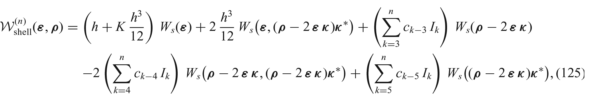
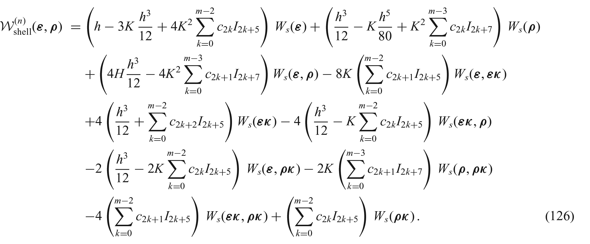
where $n$ is odd and $I_{2r}=0$ (for all $r\ge 1$ ). Similarly, for any odd integer $n=2m+1$ , we truncate the power series appearing in the coefficients of equation (124) and obtain the following equivalent (expanded) form of the strain energy density for the model of order $O(h^n)$

$$\begin{array}{c}{\mathcal{W}}_{\mathrm{shell}}^{(n)}(\mathit{\epsilon },\mathit{\rho })=(h-3K\frac{h^3}{12}+4K^2\sum _{k=0}^{m-2}{c}_{2k}{I}_{2k+5})W_s(\mathit{\epsilon })+(\frac{h^3}{12}-K\frac{h^5}{80}+K^2\sum _{k=0}^{m-3}{c}_{2k}{I}_{2k+7})W_s(\mathit{\rho })\hfill \\ +(4H\frac{h^3}{12}-4K^2\sum _{k=0}^{m-3}{c}_{2k+1}{I}_{2k+7})W_s(\mathit{\epsilon },\mathit{\rho })-8K\left(\sum _{k=0}^{m-2}{c}_{2k+1}{I}_{2k+5}\right)W_s(\mathit{\epsilon },\mathit{\epsilon }\mathit{\kappa })\hfill \\ +4(\frac{h^3}{12}+\sum _{k=0}^{m-2}{c}_{2k+2}{I}_{2k+5})W_s(\mathit{\epsilon }\mathit{\kappa })-4(\frac{h^3}{12}-K\sum _{k=0}^{m-2}{c}_{2k}{I}_{2k+5})W_s(\mathit{\epsilon }\mathit{\kappa },\mathit{\rho })\hfill \\ -2(\frac{h^3}{12}-2K\sum _{k=0}^{m-2}{c}_{2k}{I}_{2k+5})W_s(\mathit{\epsilon },\mathit{\rho }\mathit{\kappa })-2K\left(\sum _{k=0}^{m-3}{c}_{2k+1}{I}_{2k+7}\right)W_s(\mathit{\rho },\mathit{\rho }\mathit{\kappa })\hfill \\ -4\left(\sum _{k=0}^{m-2}{c}_{2k+1}{I}_{2k+5}\right)W_s(\mathit{\epsilon }\mathit{\kappa },\mathit{\rho }\mathit{\kappa })+\left(\sum _{k=0}^{m-2}{c}_{2k}{I}_{2k+5}\right)W_s(\mathit{\rho }\mathit{\kappa }).\hfill \end{array}$$

(126)

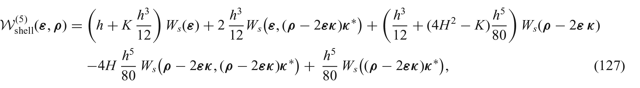
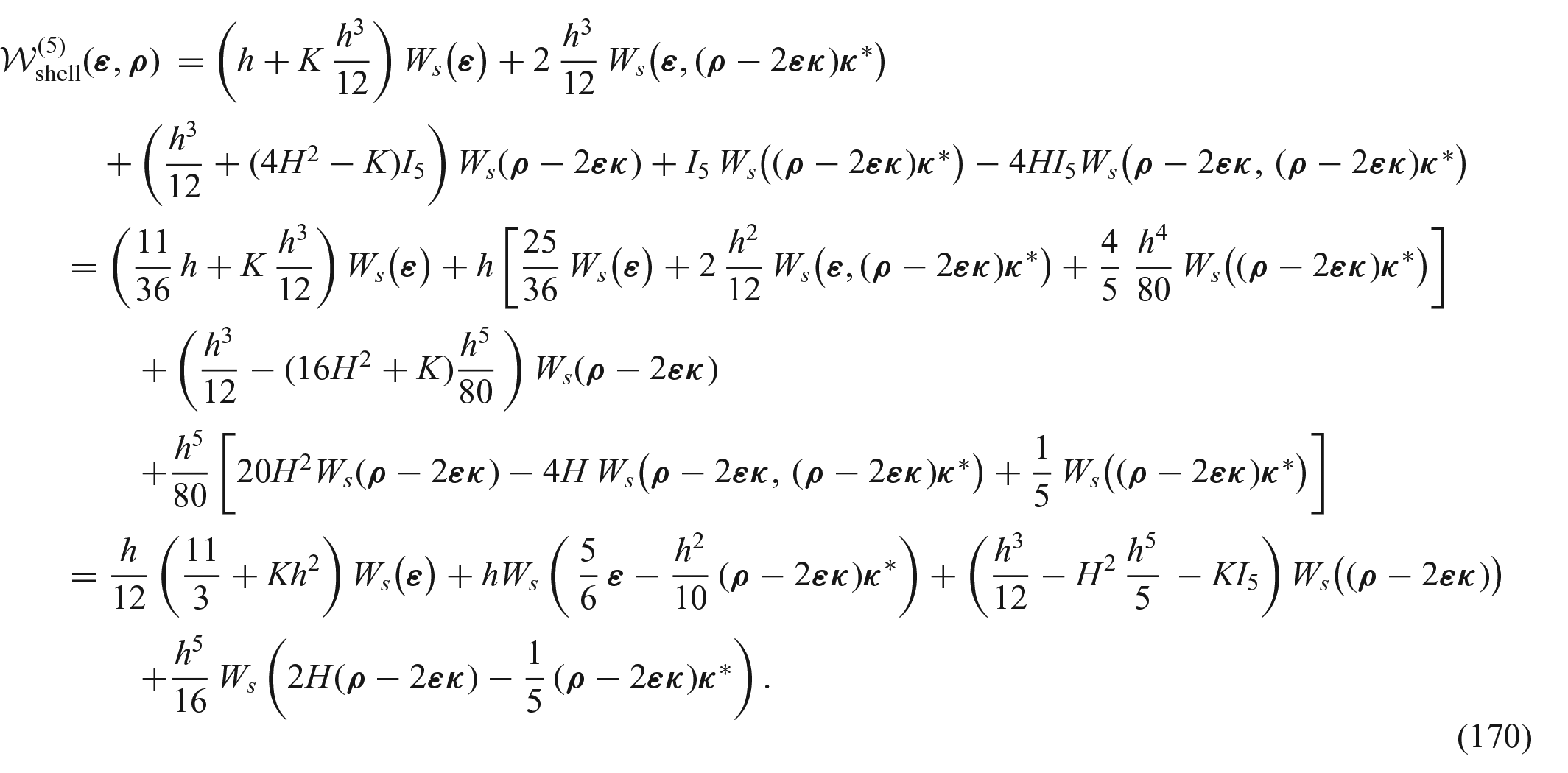
Remark: From the above relations we can readily deduce the expressions of the energies for the models of order $O(h^3)$ , $O(h^5)$ , $O(h^7)$ , etc. For instance, for $n=5$ , the condensed form (125) reduces to

$$\begin{array}{c}{\mathcal{W}}_{\mathrm{shell}}^{(5)}(\mathit{\epsilon },\mathit{\rho })=(h+K\frac{h^3}{12})W_s(\mathit{\epsilon })+2\frac{h^3}{12}{W}_s(\mathit{\epsilon },(\mathit{\rho }-2\mathit{\epsilon }\mathit{\kappa }){\mathit{\kappa }}^{*})+(\frac{h^3}{12}+(4H^2-K)\frac{h^5}{80})W_s(\mathit{\rho }-2\mathit{\epsilon }\mathit{\kappa })\hfill \\ -4H\frac{h^5}{80}{W}_s(\mathit{\rho }-2\mathit{\epsilon }\mathit{\kappa },(\mathit{\rho }-2\mathit{\epsilon }\mathit{\kappa }){\mathit{\kappa }}^{*})+\frac{h^5}{80}{W}_s((\mathit{\rho }-2\mathit{\epsilon }\mathit{\kappa }){\mathit{\kappa }}^{*}),\hfill \end{array}$$

(127)

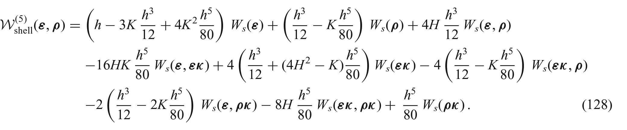
while the expanded form (126) becomes

$$\begin{array}{c}{\mathcal{W}}_{\mathrm{shell}}^{(5)}(\mathit{\epsilon }\mathit{\rho })=(h-3K\frac{h^3}{12}+4K^2\frac{h^5}{80})W_s(\mathit{\epsilon })+(\frac{h^3}{12}-K\frac{h^5}{80})W_s(\mathit{\rho })+4H\frac{h^3}{12}{W}_s(\mathit{\epsilon },\mathit{\rho })\hfill \\ -16\mathrm{HK}\frac{h^5}{80}{W}_s(\mathit{\epsilon },\mathit{\epsilon }\mathit{\kappa })+4(\frac{h^3}{12}+(4H^2-K)\frac{h^5}{80})W_s(\mathit{\epsilon }\mathit{\kappa })-4(\frac{h^3}{12}-K\frac{h^5}{80})W_s(\mathit{\epsilon }\mathit{\kappa },\mathit{\rho })\hfill \\ -2(\frac{h^3}{12}-2K\frac{h^5}{80})W_s(\mathit{\epsilon },\mathit{\rho }\mathit{\kappa })-8H\frac{h^5}{80}{W}_s(\mathit{\epsilon }\mathit{\kappa },\mathit{\rho }\mathit{\kappa })+\frac{h^5}{80}{W}_s(\mathit{\rho }\mathit{\kappa }).\hfill \end{array}$$

(128)

Note that relations (127) and (128) are equivalent.

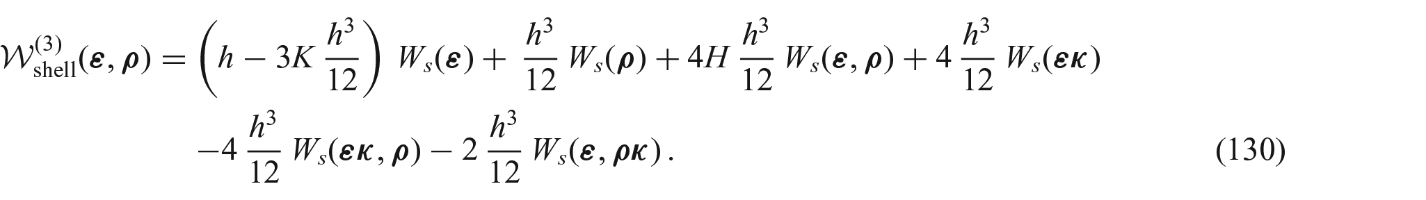
If we keep only the terms up to the power $h^3$ , then we get the following condensed expression for the model of order $O(h^3)$

$$\begin{array}{c}{\mathcal{W}}_{\mathrm{shell}}^{(3)}(\mathit{\epsilon },\mathit{\rho })=(h+K\frac{h^3}{12})W_s(\mathit{\epsilon })+\frac{h^3}{12}{W}_s(\mathit{\rho }-2\mathit{\epsilon }\mathit{\kappa })+2\frac{h^3}{12}{W}_s(\mathit{\epsilon },(\mathit{\rho }-2\mathit{\epsilon }\mathit{\kappa }){\mathit{\kappa }}^{*}),\hfill \end{array}$$

(129)

which can be written equivalently in the expanded form

$$\begin{array}{c}{\mathcal{W}}_{\mathrm{shell}}^{(3)}(\mathit{\epsilon },\mathit{\rho })=(h-3K\frac{h^3}{12})W_s(\mathit{\epsilon })+\frac{h^3}{12}{W}_s(\mathit{\rho })+4H\frac{h^3}{12}{W}_s(\mathit{\epsilon },\mathit{\rho })+4\frac{h^3}{12}{W}_s(\mathit{\epsilon }\mathit{\kappa })\hfill \\ -4\frac{h^3}{12}{W}_s(\mathit{\epsilon }\mathit{\kappa },\mathit{\rho })-2\frac{h^3}{12}{W}_s(\mathit{\epsilon },\mathit{\rho }\mathit{\kappa }).\hfill \end{array}$$

(130)

In the classical (Koiter) theory of linear elastic shells, the coupling part of the energy and all the terms of order $O(\epsilon \kappa )$ are neglected (where $\epsilon =\parallel \mathit{\epsilon }\parallel$ and $\kappa =\underset{\mathrm{\Omega }}{max}\{|{\kappa }_1|,|{\kappa }_2|\}$ ). Also, the term $K\frac{h^3}{12}$ is considered negligible in comparison to $h$ , since we have

$$|K{h}^2|=|{\kappa }_{1}h|·|{\kappa }_{2}h|\mathrm{and}|{\kappa }_{\alpha }h|<<1.$$

Under these approximations, the strain energy density (130) reduces to the linear Koiter model given by relation (26).

5. Coercivity of the strain energy function

In this Section, we show the coercivity of the energy density function, both for the shell model of order $O(h^n)$ and for the general shell model (when $n\to \infty$ ). Note that the coercivity property is crucial to establish the existence of solutions to the shell equations.

We assume throughout that the Lamé constants satisfy the usual conditions

$$\mu >0\mathrm{and}3\lambda +2\mu >0,$$

(131)

which assure the positive definiteness of the quadratic form $W_{3\mathrm{d}}(\mathit{X})$ defined by equation (30). We denote by $c_m$ and $c_M$ the positive constants

$$c_m=\underset{\mathrm{\Omega }}{min}\{\mu ,\frac{\mu (3\lambda +2\mu )}{\lambda +2\mu }\},c_M=\underset{\mathrm{\Omega }}{max}\{\mu ,\frac{\mu (3\lambda +2\mu )}{\lambda +2\mu }\}.$$

(132)

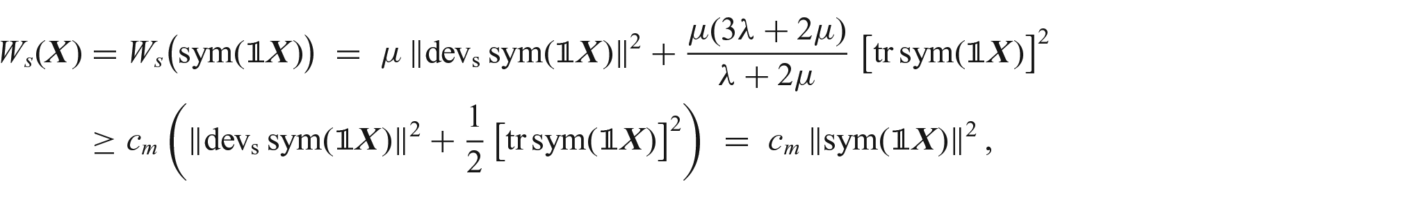
Let us show first that the quadratic form $W_s(\mathit{X})$ defined by equation (25) satisfies the relation

$$c_m\parallel \mathrm{sym}(\mathbb{1}\mathit{X}){\parallel }^2\le W_s(\mathit{X})\le c_M\parallel \mathrm{sym}(\mathbb{1}\mathit{X}){\parallel }^2,\mathrm{for}\mathrm{any}\mathit{X}=X_{i\alpha }{\mathit{a}}^i\otimes {\mathit{a}}^{\alpha }.$$

(133)

Indeed, if we consider the surface deviator operator ${\mathrm{dev}}_s$ defined in the work by Bîrsan and Neff [21] by

$$\mathrm{de}{\mathrm{v}}_{\mathrm{s}}\mathit{X}=\mathit{X}-\frac{1}{2}(\mathrm{tr}\mathit{X})\mathbb{1},$$

(134)

then we have (see f. (104) from the work by Bîrsan and Neff [21])

$$\parallel \mathrm{sym}\mathit{X}{\parallel }^2=\parallel \mathrm{de}{\mathrm{v}}_{\mathrm{s}}\mathrm{sym}\mathit{X}{\parallel }^2+\frac{1}{2}(\mathrm{tr}\mathit{X}{)}^2,\mathrm{for}\mathrm{any}\mathit{X}=X_{i\alpha }{\mathit{a}}^i\otimes {\mathit{a}}^{\alpha }.$$

(135)

Using this relation in the definition (25), we can estimate

$$\begin{array}{c}{W}_s(\mathit{X})=W_s(\mathrm{sym}(\mathbb{1}\mathit{X}))=\mu \parallel \mathrm{de}{\mathrm{v}}_{\mathrm{s}}\mathrm{sym}(\mathbb{1}\mathit{X}){\parallel }^2+\frac{\mu (3\lambda +2\mu )}{\lambda +2\mu }[\mathrm{tr}\mathrm{sym}(\mathbb{1}\mathit{X}){]}^2\hfill \\ \ge c_m(\parallel \mathrm{de}{\mathrm{v}}_{\mathrm{s}}\mathrm{sym}(\mathbb{1}\mathit{X}){\parallel }^2+\frac{1}{2}{[\mathrm{tr}\mathrm{sym}(\mathbb{1}\mathit{X})]}^2)=c_m\parallel \mathrm{sym}(\mathbb{1}\mathit{X}){\parallel }^2,\hfill \end{array}$$

so the first inequality in equation (133) is proved. Similarly, we can also show the second inequality in equation (133).

For future use, let us denote by ${\kappa }_M$ the following maximum

$${\kappa }_M=\underset{\mathrm{\Omega }}{max}\{|{\kappa }_1|,|{\kappa }_2|\}=\underset{\mathrm{\Omega }}{max}\{\frac{1}{R_1},\frac{1}{R_2}\},$$

(136)

where $R_{\alpha }=|{\kappa }_{\alpha }{|}^{-1}$ are the curvature radii of the midsurface.

5.1. Coercivity for the general shell model ( $n\to \infty$ )

Let us establish the following coercivity result.

Proposition 4. Assume that the principal curvatures ${\kappa }_1,{\kappa }_2$ satisfy the condition $|{\kappa }_{\alpha }|h<\frac{17}{40}=0.425$ . Then, the strain energy density function ${\mathcal{W}}_{\mathrm{shell}}(\mathit{\epsilon },\mathit{\rho })$ defined by equation (122) satisfy the inequality

$${\mathcal{W}}_{\mathrm{shell}}(\mathit{\epsilon },\mathit{\rho })\ge \frac{c_{m}h}{1000}(\parallel \mathit{\epsilon }{\parallel }^2+\frac{h^2}{48}\parallel \mathit{\rho }{\parallel }^2),$$

(137)

so it is coercive.

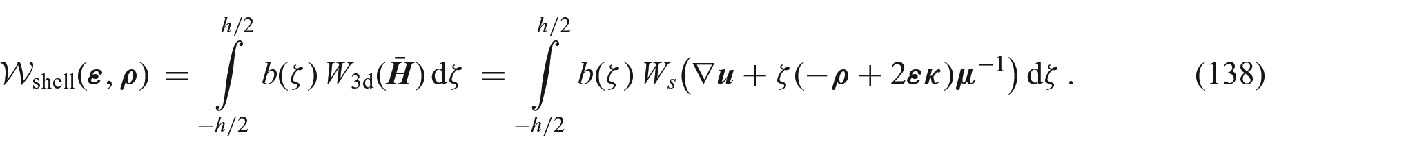
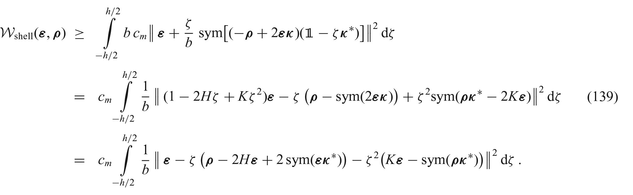
Proof. In view of the derivation procedure for the shell model, we see that the strain energy density is obtained by integration over the thickness from the following integral (see equations (83), (84), and (120))

$${\mathcal{W}}_{\mathrm{shell}}(\mathit{\epsilon },\mathit{\rho })=\underset{-h/2}{\overset{h/2}{\int }}b(\zeta )W_{3\mathrm{d}}(\overline{\mathit{H}})\mathrm{d}\zeta =\underset{-h/2}{\overset{h/2}{\int }}b(\zeta )W_s(\nabla \mathit{u}+\zeta (-\mathit{\rho }+2\mathit{\epsilon }\mathit{\kappa }){\mathit{\mu }}^{-1})\mathrm{d}\zeta .$$

(138)

Using here the estimate (133) and the relation ${\mathit{\mu }}^{-1}=\frac{1}{b}(\mathbb{1}-\zeta {\mathit{\kappa }}^{*}),$ we can write the inequalities

$$\begin{array}{c}{\mathcal{W}}_{\mathrm{shell}}(\mathit{\epsilon },\mathit{\rho })\ge \underset{-h/2}{\overset{h/2}{\int }}b{c}_m\parallel \mathit{\epsilon }+\frac{\zeta }{b}\mathrm{sym}[(-\mathit{\rho }+2\mathit{\epsilon }\mathit{\kappa })(\mathbb{1}-\zeta {\mathit{\kappa }}^{*})]{\parallel }^2\mathrm{d}\zeta \hfill \\ \multicolumn{1}{c}{=c_m\underset{-h/2}{\overset{h/2}{\int }}\frac{1}{b}\parallel (1-2H\zeta +K{\zeta }^2)\mathit{\epsilon }-\zeta (\mathit{\rho }-\mathrm{sym}(2\mathit{\epsilon }\mathit{\kappa }))+{\zeta }^2\mathrm{sym}(\mathit{\rho }{\mathit{\kappa }}^{*}-2K\mathit{\kappa }){\parallel }^2\mathrm{d}\zeta }\\ \multicolumn{1}{c}{=c_m\underset{-h/2}{\overset{h/2}{\int }}\frac{1}{b}\parallel \mathit{\epsilon }-\zeta (\mathit{\rho }-2H\mathit{\epsilon }+2\mathrm{sym}(\mathit{\epsilon }{\mathit{\kappa }}^{*}))-{\zeta }^2(K\mathit{\epsilon }-\mathrm{sym}(\mathit{\rho }{\mathit{\kappa }}^{*})){\parallel }^2\mathrm{d}\zeta .}\end{array}$$

(139)

The last integrand can be transformed as follows:

$$\begin{array}{c}\parallel \mathit{\epsilon }-\zeta (\mathit{\rho }-2H\mathit{\epsilon }+2\mathrm{sym}(\mathit{\epsilon }{\mathit{\kappa }}^{*}))-{\zeta }^2(K\mathit{\epsilon }-\mathrm{sym}(\mathit{\rho }{\mathit{\kappa }}^{*})){\parallel }^2\hfill \\ \multicolumn{1}{c}{=\parallel \mathit{\epsilon }{\parallel }^2-2\zeta \mathit{\epsilon }·(\mathit{\rho }-2H\mathit{\epsilon }+2\mathrm{sym}(\mathit{\epsilon }{\mathit{\kappa }}^{*}))-2{\zeta }^2\mathit{\epsilon }·(K\mathit{\epsilon }-\mathrm{sym}(\mathit{\rho }{\mathit{\kappa }}^{*}))+{\zeta }^4\parallel K\mathit{\epsilon }-\mathrm{sym}(\mathit{\rho }{\mathit{\kappa }}^{*}){\parallel }^2}\\ \multicolumn{1}{c}{+{\zeta }^2\parallel \mathit{\rho }-2H\mathit{\epsilon }+2\mathrm{sym}(\mathit{\epsilon }{\mathit{\kappa }}^{*}){\parallel }^2+2{\zeta }^3(\mathit{\rho }-2H\mathit{\epsilon }+2\mathrm{sym}(\mathit{\epsilon }{\mathit{\kappa }}^{*}))·(K\mathit{\epsilon }-\mathrm{sym}(\mathit{\rho }{\mathit{\kappa }}^{*})).}\end{array}$$

(140)

Now, from $|{\kappa }_{\alpha }|h<1$ it follows $|{\kappa }_{\alpha }\zeta |<\frac{1}{2}$ , so we have

$$\frac{1}{b(\zeta )}=\frac{1}{(1-{\kappa }_1\zeta )(1-{\kappa }_2\zeta )}>\frac{1}{4}.$$

(141)

Then, we insert equations (140) and (141) into equation (139) and integrate over the thickness. Since $I_2=0$ and $I_4=0$ , we obtain

$$\begin{array}{c}{\mathcal{W}}_{\mathrm{shell}}(\mathit{\epsilon },\mathit{\rho })\ge \frac{c_m}{4}[h\parallel \mathit{\epsilon }{\parallel }^2-2\frac{h^3}{12}\mathit{\epsilon }·(K\mathit{\epsilon }-\mathrm{sym}(\mathit{\rho }{\mathit{\kappa }}^{*}))+\frac{h^3}{12}\parallel \mathit{\rho }-2H\mathit{\epsilon }+2\mathrm{sym}(\mathit{\epsilon }{\mathit{\kappa }}^{*}){\parallel }^2]\hfill \\ \multicolumn{1}{c}{=\frac{c_m}{4}[(h-K\frac{h^3}{6})\parallel \mathit{\epsilon }{\parallel }^2+\frac{h^3}{6}\mathit{\epsilon }·(\mathit{\rho }{\mathit{\kappa }}^{*})+\frac{h^3}{12}\parallel \mathit{\rho }-2H\mathit{\epsilon }+2\mathrm{sym}(\mathit{\epsilon }{\mathit{\kappa }}^{*}){\parallel }^2].}\end{array}$$

(142)

For the last term we can write the inequality

$$\begin{array}{c}\parallel \mathit{\rho }-2H\mathit{\epsilon }+2\mathrm{sym}(\mathit{\epsilon }{\mathit{\kappa }}^{*}){\parallel }^2=\parallel \mathit{\rho }{\parallel }^2-4\mathit{\rho }·(H\mathit{\epsilon }-\mathrm{sym}(\mathit{\epsilon }{\mathit{\kappa }}^{*}))+4\parallel H\mathit{\epsilon }-\mathrm{sym}(\mathit{\epsilon }{\mathit{\kappa }}^{*}){\parallel }^2\hfill \\ \multicolumn{1}{c}{\ge \parallel \mathit{\rho }{\parallel }^2-4H\mathit{\rho }·\mathit{\epsilon }+4\mathit{\rho }·(\mathit{\epsilon }{\mathit{\kappa }}^{*})=\parallel \mathit{\rho }{\parallel }^2-4H\mathit{\epsilon }·\mathit{\rho }+4\mathit{\epsilon }·(\mathit{\rho }{\mathit{\kappa }}^{*}).}\end{array}$$

(143)

Using relation (143) in equation (142), we deduce

$${\mathcal{W}}_{\mathrm{shell}}(\mathit{\epsilon },\mathit{\rho })\ge \frac{c_{m}h}{4}[(1-K\frac{h^2}{6})\parallel \mathit{\epsilon }{\parallel }^2+\frac{h^2}{12}\parallel \mathit{\rho }{\parallel }^2-H\frac{h^2}{3}\mathit{\epsilon }·\mathit{\rho }+\frac{h^2}{2}\mathit{\epsilon }·(\mathit{\rho }{\mathit{\kappa }}^{*})].$$

(144)

By the Cauchy–Schwarz inequality we have

$$|\mathit{\epsilon }·\mathit{\rho }|\le \parallel \mathit{\epsilon }\parallel ·\parallel \mathit{\rho }\parallel \mathrm{and}|\mathit{\epsilon }·(\mathit{\rho }{\mathit{\kappa }}^{*})|\le \parallel \mathit{\epsilon }\parallel ·\parallel \mathit{\rho }{\mathit{\kappa }}^{*}\parallel$$

(145)

Furthermore, let us prove that

$$\parallel \mathit{\rho }{\mathit{\kappa }}^{*}\parallel \le 2{\kappa }_M\parallel \mathit{\rho }\parallel .$$

(146)

To this aim, we use the spectral representation of the initial curvature tensor $\mathit{\kappa }$ in the form

$$\mathit{\kappa }={\kappa }_1{\mathit{u}}_1\otimes {\mathit{u}}_1+{\kappa }_2{\mathit{u}}_2\otimes {\mathit{u}}_2,$$

(147)

where ${\mathit{u}}_1$ and ${\mathit{u}}_2$ are the orthonormal principal vectors. Then, we have $\mathbb{1}={\mathit{u}}_1\otimes {\mathit{u}}_1+{\mathit{u}}_2\otimes {\mathit{u}}_2$ and the cofactor ${\mathit{\kappa }}^{*}$ can be written as

$$\begin{array}{c}{\mathit{\kappa }}^{*}=H\mathbb{1}+(H\mathbb{1}-\mathit{\kappa })=H\mathbb{1}+[\frac{{\kappa }_1+{\kappa }_2}{2}({\mathit{u}}_1\otimes {\mathit{u}}_1+{\mathit{u}}_2\otimes {\mathit{u}}_2)-({\kappa }_1{\mathit{u}}_1\otimes {\mathit{u}}_1+{\kappa }_2{\mathit{u}}_2\otimes {\mathit{u}}_2)]\hfill \\ =H\mathbb{1}+\frac{{\kappa }_1-{\kappa }_2}{2}({\mathit{u}}_2\otimes {\mathit{u}}_2-{\mathit{u}}_1\otimes {\mathit{u}}_1)=H\mathbb{1}+\frac{{\kappa }_1-{\kappa }_2}{2}\mathit{\delta },\hfill \end{array}$$

(148)

where we denote

$$\mathit{\delta }:={\mathit{u}}_2\otimes {\mathit{u}}_2-{\mathit{u}}_1\otimes {\mathit{u}}_1.$$

Thus, we have

$$\mathit{\rho }{\mathit{\kappa }}^{*}=H\mathit{\rho }+\frac{{\kappa }_1-{\kappa }_2}{2}\mathit{\rho }\mathit{\delta }$$

(149)

and we can estimate

$$\parallel \mathit{\rho }{\mathit{\kappa }}^{*}{\parallel }^2=\parallel H\mathit{\rho }+\frac{{\kappa }_1-{\kappa }_2}{2}\mathit{\rho }\mathit{\delta }{\parallel }^2\le 2H^2\parallel \mathit{\rho }{\parallel }^2+2(H^2-K)\parallel \mathit{\rho }\mathit{\delta }{\parallel }^2,$$

(150)

since

$${\left(\frac{{\kappa }_1-{\kappa }_2}{2}\right)}^2={\left(\frac{{\kappa }_1+{\kappa }_2}{2}\right)}^2-{\kappa }_1{\kappa }_2=H^2-K.$$

Using notation (136) we have

$$H^2={\left(\frac{{\kappa }_1+{\kappa }_2}{2}\right)}^2\le \frac{{\kappa }_1^2+{\kappa }_2^2}{2}\le {\kappa }_M^2\mathrm{and}{H}^2-K={\left(\frac{{\kappa }_1-{\kappa }_2}{2}\right)}^2\le \frac{{\kappa }_1^2+{\kappa }_2^2}{2}\le {\kappa }_M^2,$$

(151)

so inequality (150) infers

$$\parallel \mathit{\rho }{\mathit{\kappa }}^{*}{\parallel }^2\le 2{\kappa }_M^2(\parallel \mathit{\rho }{\parallel }^2+\parallel \mathit{\rho }\mathit{\delta }{\parallel }^2).$$

(152)

Since the vectors ${\mathit{u}}_1$ and ${\mathit{u}}_2$ are orthogonal, we can write

$$\begin{array}{c}\parallel \mathit{\rho }\mathit{\delta }{\parallel }^2=\parallel \mathit{\rho }({\mathit{u}}_2\otimes {\mathit{u}}_2-{\mathit{u}}_1\otimes {\mathit{u}}_1){\parallel }^2=\parallel \mathit{\rho }{\mathit{u}}_2\otimes {\mathit{u}}_2{\parallel }^2+\parallel \mathit{\rho }{\mathit{u}}_1\otimes {\mathit{u}}_1{\parallel }^2\hfill \\ \multicolumn{1}{c}{=\parallel \mathit{\rho }({\mathit{u}}_1\otimes {\mathit{u}}_1+{\mathit{u}}_2\otimes {\mathit{u}}_2){\parallel }^2=\parallel \mathit{\rho }{\parallel }^2,}\end{array}$$

(153)

so inequality (152) reduces to

$$\parallel \mathit{\rho }{\mathit{\kappa }}^{*}{\parallel }^2\le 4{\kappa }_M^2\parallel \mathit{\rho }{\parallel }^2,$$

which means that relation (146) holds true.

Using inequalities (145) and (146) in equation (144), we deduce the estimate

$${\mathcal{W}}_{\mathrm{shell}}(\mathit{\epsilon },\mathit{\rho })\ge \frac{c_{m}h}{4}[(1-K\frac{h^2}{6})\parallel \mathit{\epsilon }{\parallel }^2+\frac{h^2}{12}\parallel \mathit{\rho }{\parallel }^2-(H-3{\kappa }_M)\frac{h^2}{3}\parallel \mathit{\epsilon }\parallel ·\parallel \mathit{\rho }\parallel ].$$

(154)

Then, for any scalar $\alpha \in (0,1)$ we can write

$$\begin{array}{c}{\mathcal{W}}_{\mathrm{shell}}(\mathit{\epsilon },\mathit{\rho })\ge \frac{c_{m}h}{4}[(1-\alpha -K\frac{h^2}{6})\parallel \mathit{\epsilon }{\parallel }^2+\frac{h^2}{12}(1-{(H-3{\kappa }_M)}^2\frac{h^2}{3\alpha })\parallel \mathit{\rho }{\parallel }^2\hfill \\ \multicolumn{1}{c}{+{(\sqrt{\alpha }\parallel \mathit{\epsilon }\parallel -(H-3{\kappa }_M)\frac{h^2}{6\sqrt{\alpha }}\parallel \mathit{\rho }\parallel )}^2],}\end{array}$$

so

$${\mathcal{W}}_{\mathrm{shell}}(\mathit{\epsilon },\mathit{\rho })\ge \frac{c_{m}h}{4}[(1-\alpha -K\frac{h^2}{6})\parallel \mathit{\epsilon }{\parallel }^2+\frac{h^2}{12}(1-{(H-3{\kappa }_M)}^2\frac{h^2}{3\alpha })\parallel \mathit{\rho }{\parallel }^2].$$

(155)

Let us choose now the constant $\alpha \in (0,1)$ such that the above coefficients of $\parallel \mathit{\epsilon }{\parallel }^2$ and $\parallel \mathit{\rho }{\parallel }^2$ be positive. From the hypothesis $|{\kappa }_{\alpha }|h<\frac{17}{40}$ , it follows that

$${\kappa }_{M}h<\frac{17}{40},|H|h\le \frac{1}{2}(|{\kappa }_{1}h|+|{\kappa }_{2}h|)<\frac{17}{40}\mathrm{and}|K|h^2=|{\kappa }_{1}h|·|{\kappa }_{2}h|<{\left(\frac{17}{40}\right)}^2,$$

so we have

$$1-K\frac{h^2}{6}>1-\frac{1}{6}{\left(\frac{17}{40}\right)}^2>0.969$$

and

$$(H-3{\kappa }_M)\frac{h^2}{3}\le \frac{1}{3}(|H|h+3{\kappa }_{M}h{)}^2<\frac{1}{3}{(4·\frac{17}{40})}^2=\frac{1}{3}1.7^2<0.964.$$

Thus, if we choose $\alpha =0.965$ , then we have

$$1-\alpha -K\frac{h^2}{6}>0.004\mathrm{and}1-(H-3{\kappa }_M{)}^2\frac{h^2}{3\alpha }>1-\frac{0.964}{0.965}>0.001.$$

(156)

Finally, we insert these inequalities into equation (155) and obtain that estimate (137) holds true. The proof is complete. ■

Remark: The coercivity property established in Proposition 4 is important, since it allows one to prove the existence of weak solutions to the equilibrium equations for the general model of linear elastic shells. Indeed, using the method presented in the work by Ciarlet [19, 20, 22], the existence proof relies on the coercivity of ${\mathcal{W}}_{\mathrm{shell}}(\mathit{\epsilon },\mathit{\rho })$ , on the Korn inequality for the midsurface and on the Lax–Milgram theorem.

5.2. Coercivity result for the shell model of order $O(h^n)$ with $n\ge$ 5

The expression of the strain energy density ${\mathcal{W}}_{\mathrm{shell}}^{(n)}(\mathit{\epsilon },\mathit{\rho })$ is given by equation (126), or equivalently (125). Notice that in the case $n=3$ the last two terms are missing in expression (125). These terms play an important role in the coercivity proof. Therefore, we consider first the case $n\ge 5$ and establish some auxiliary results.

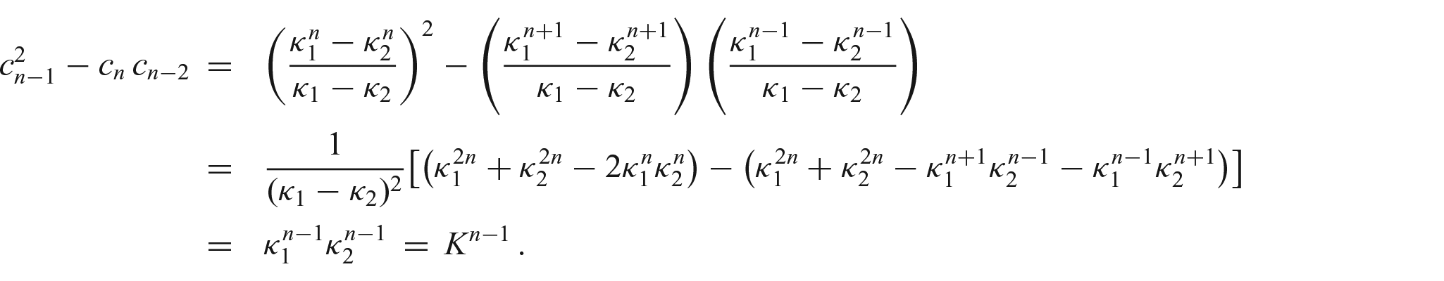
Lemma 5. (i) Let $c_n$ be the coefficients of the series expansion of $\frac{1}{b(\zeta )}$ given by equation (90). Then, it holds

$$c_{2m}>0\mathrm{for}\mathrm{any}m\in \mathbb{N}.$$

(157)

The equality $c_{2m}=0$ takes place if and only if ${\kappa }_1={\kappa }_2=0$ .

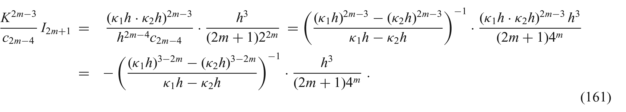
(ii) For the coefficients $c_n$ and for any $n\ge 2$ , the following relation holds

$$c_{n-1}^2-c_n{c}_{n-2}=K^{n-1}.$$

(158)

(iii) If the condition $|{\kappa }_{\alpha }h|<\frac{1}{2}$ is satisfied, then the following estimate holds for any $m\ge 2$ :

$$\left|\frac{K^{2m-3}}{c_{2m-4}}{I}_{2m+1}\right|<\frac{h^3}{(2m+1)4^{2m-1}}.$$

(159)

Proof. (i) In view of relation (97) we see that

$$c_n=\{\begin{array}{cc}\frac{{\kappa }_1^{n+1}-{\kappa }_2^{n+1}}{{\kappa }_1-{\kappa }_2},\hfill & \mathrm{if}{\kappa }_1\ne {\kappa }_2,\hfill \\ \multicolumn{1}{c}{(n+1){\kappa }_1^n,}& \mathrm{if}{\kappa }_1={\kappa }_2,\hfill \end{array}$$

(160)

so we deduce $c_{2m}>0$ , since the function $x\mapsto x^{2m+1}$ is strictly monotonically increasing.

(ii) Using relation (160), we can write (in case ${\kappa }_1\ne {\kappa }_2$ )

$$\begin{array}{c}{c}_{n-1}^2-c_n{c}_{n-2}={\left(\frac{{\kappa }_1^n-{\kappa }_2^n}{{\kappa }_1-{\kappa }_2}\right)}^2-\left(\frac{{\kappa }_1^{n+1}-{\kappa }_2^{n+1}}{{\kappa }_1-{\kappa }_2}\right)\left(\frac{{\kappa }_1^{n-1}-{\kappa }_2^{n-1}}{{\kappa }_1-{\kappa }_2}\right)\hfill \\ \multicolumn{1}{c}{=\frac{1}{{({\kappa }_1-{\kappa }_2)}^2}[({\kappa }_1^{2n}+{\kappa }_2^{2n}-2{\kappa }_1^n{\kappa }_2^n)-({\kappa }_1^{2n}+{\kappa }_2^{2n}-{\kappa }_1^{n+1}{\kappa }_2^{n-1}-{\kappa }_1^{n-1}{\kappa }_2^{n+1})]}\\ \multicolumn{1}{c}{={\kappa }_1^{n-1}{\kappa }_2^{n-1}=K^{n-1}.}\end{array}$$

In the case ${\kappa }_1={\kappa }_2$ , we obtain directly

$$c_{n-1}^2-c_n{c}_{n-2}=(n{\kappa }_1^{n-1}{)}^2-(n+1)(n-1){\kappa }_1^n{\kappa }_1^{n-2}={\kappa }_1^{2n-2}=({\kappa }_1{\kappa }_2{)}^{n-1}=K^{n-1}.$$

(iii) The inequality is true in the case ${\kappa }_1={\kappa }_2$ , since we have

$$\begin{array}{c}\left|\frac{K^{2m-3}}{c_{2m-4}}{I}_{2m+1}\right|=|\frac{{\kappa }_1^{4m-6}}{(2m-3){\kappa }_1^{2m-4}}·\frac{h^{2m+1}}{(2m+{1)2}^{2m}}|=\frac{|{\kappa }_{1}h{|}^{2m-2}}{2m-3}·\frac{h^3}{(2m+{1)2}^{2m}}<\frac{h^3}{(2m+1)4^{2m-1}}.\hfill \end{array}$$

In the case ${\kappa }_1\ne {\kappa }_2$ , we can write

$$\begin{array}{c}\frac{K^{2m-3}}{c_{2m-4}}{I}_{2m+1}=\frac{{({\kappa }_{1}h·{\kappa }_{2}h)}^{2m-3}}{h^{2m-4}{c}_{2m-4}}·\frac{h^3}{(2m+{1)2}^{2m}}={\left(\frac{{({\kappa }_{1}h)}^{2m-3}-{({\kappa }_{2}h)}^{2m-3}}{{\kappa }_{1}h-{\kappa }_{2}h}\right)}^{-1}·\frac{{({\kappa }_{1}h·{\kappa }_{2}h)}^{2m-3}{h}^3}{(2m+{1)4}^m}\hfill \\ \multicolumn{1}{c}{=-{\left(\frac{{({\kappa }_{1}h)}^{3-2m}-{({\kappa }_{2}h)}^{3-2m}}{{\kappa }_{1}h-{\kappa }_{2}h}\right)}^{-1}·\frac{h^3}{(2m+{1)4}^m}.}\end{array}$$

(161)

Next, if we denote the function

$$g_m(x):=\frac{1}{x^{2m-3}}\mathrm{for}\mathrm{any}x\in (-\frac{1}{2},\frac{1}{2})\mathrm{and}m\ge 2,$$

(162)

then relation (161) infers

$$\left|\frac{K^{2m-3}}{c_{2m-4}}{I}_{2m+1}\right|={\left|\frac{g_m({\kappa }_{1}h)-g_m({\kappa }_{2}h)}{{\kappa }_{1}h-{\kappa }_{2}h}\right|}^{-1}·\frac{h^3}{(2m+1)4^m}.$$

(163)

One can easily prove that

$$\left|\frac{g_m(x)-g_m(y)}{x-y}\right|>4^{m-1}\mathrm{for}\mathrm{any}x,y\in (-\frac{1}{2},\frac{1}{2})\backslash \{0\}\mathrm{with}x\ne y.$$

(164)

Indeed, if $\mathrm{xy}>0$ , then there exists a value $\xi$ between $x$ and $y$ such that

$$\left|\frac{g_m(x)-g_m(y)}{x-y}\right|=|g_m^{\prime }(\xi )|=\left|\frac{2m-3}{{\xi }^{2m-2}}\right|>(2m-3)2^{2m-2}\ge 4^{m-1}.$$

In the case when $\mathrm{xy}<0$ , let us assume without loss of generality that $x<0<y$ . Then, we have

$$g_m(x)<g_m(-\frac{1}{2})<0<g_m\left(\frac{1}{2}\right)<g_m(y),$$

so it follows

$$\left|\frac{g_m(x)-g_m(y)}{x-y}\right|=\frac{g_m(y)-g_m(x)}{y-x}>\frac{g_m\left(\frac{1}{2}\right)-g_m(-\frac{1}{2})}{\frac{1}{2}+\frac{1}{2}}=2g_m\left(\frac{1}{2}\right)=4^{m-1}.$$

In both cases, inequality (164) is proved. Using relation (164) in equation (163), we obtain the estimate (159). The proof is complete. ■

Let us show now the following coercivity result.

Proposition 6. Assume that the reference midsurface satisfies the condition $|{\kappa }_{\alpha }|h<\frac{1}{2}$ . Then, the strain energy density ${\mathcal{W}}_{\mathrm{shell}}^{(n)}(\mathit{\epsilon },\mathit{\rho })$ given for $n\ge 5$ by relation (126) (or equivalently (125)) is coercive. The following inequality holds for any $n\ge 5$ :

$${\mathcal{W}}_{\mathrm{shell}}^{(n)}(\mathit{\epsilon },\mathit{\rho })\ge \frac{c_{m}h}{10}(\parallel \mathit{\epsilon }{\parallel }^2+\frac{h^2}{5}\parallel \mathit{\rho }{\parallel }^2).$$

(165)

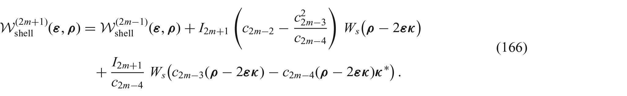
Proof. We establish first a recurrence relation for the energy functions ${\mathcal{W}}_{\mathrm{shell}}^{(n)}(\mathit{\epsilon },\mathit{\rho })$ : for any $m\ge 3$ it holds

$$\begin{array}{c}{\mathcal{W}}_{\mathrm{shell}}^{(2m+1)}(\mathit{\epsilon },\mathit{\rho })={\mathcal{W}}_{\mathrm{shell}}^{(2m-1)}(\mathit{\epsilon },\mathit{\rho })+I_{2m+1}(c_{2m-2}-\frac{c_{2m-3}^2}{c_{2m-4}})W_s(\mathit{\rho }-2\mathit{\epsilon }\mathit{\kappa })\hfill \\ \multicolumn{1}{c}{+\frac{I_{2m+1}}{c_{2m-4}}{W}_s(c_{2m-3}(\mathit{\rho }-2\mathit{\epsilon }\mathit{\kappa })-c_{2m-4}(\mathit{\rho }-2\mathit{\epsilon }\mathit{\kappa }){\mathit{\kappa }}^{*}).}\end{array}$$

(166)

Indeed, in view of equation (125), we can write the difference

$$\begin{array}{c}{\mathcal{W}}_{\mathrm{shell}}^{(2m+1)}(\mathit{\epsilon },\mathit{\rho })-{\mathcal{W}}_{\mathrm{shell}}^{(2m-1)}(\mathit{\epsilon },\mathit{\rho })=c_{2m-2}{I}_{2m+1}{W}_s(\mathit{\rho }-2\mathit{\epsilon }\mathit{\kappa })-2c_{2m-3}{I}_{2m+1}{W}_s(\mathit{\rho }-2\mathit{\epsilon }\mathit{\kappa },(\mathit{\rho }-2\mathit{\epsilon }\mathit{\kappa }){\mathit{\kappa }}^{*})\hfill \\ \multicolumn{1}{c}{+c_{2m-4}{I}_{2m+1}{W}_s((\mathit{\rho }-2\mathit{\epsilon }\mathit{\kappa }){\mathit{\kappa }}^{*})=I_{2m+1}(c_{2m-2}-\frac{c_{2m-3}^2}{c_{2m-4}})W_s(\mathit{\rho }-2\mathit{\epsilon }\mathit{\kappa })}\\ \multicolumn{1}{c}{+\frac{I_{2m+1}}{c_{2m-4}}[c_{2m-3}^2{W}_s(\mathit{\rho }-2\mathit{\epsilon }\mathit{\kappa })-2c_{2m-3}{c}_{2m-4}{W}_s(\mathit{\rho }-2\mathit{\epsilon }\mathit{\kappa },(\mathit{\rho }-2\mathit{\epsilon }\mathit{\kappa }){\mathit{\kappa }}^{*})+c_{2m-4}^2{W}_s((\mathit{\rho }-2\mathit{\epsilon }\mathit{\kappa }){\mathit{\kappa }}^{*})],}\end{array}$$

so the recurrence relation (166) holds true. Hence, using Lemma 5 (i) we deduce

$${\mathcal{W}}_{\mathrm{shell}}^{(2m+1)}(\mathit{\epsilon },\mathit{\rho })\ge {\mathcal{W}}_{\mathrm{shell}}^{(2m-1)}(\mathit{\epsilon },\mathit{\rho })+I_{2m+1}(c_{2m-2}-\frac{c_{2m-3}^2}{c_{2m-4}})W_s(\mathit{\rho }-2\mathit{\epsilon }\mathit{\kappa }).$$

(167)

Since this inequality holds for any $m\ge 3$ , we obtain inductively

$${\mathcal{W}}_{\mathrm{shell}}^{(2m+1)}(\mathit{\epsilon },\mathit{\rho })\ge {\mathcal{W}}_{\mathrm{shell}}^{(5)}(\mathit{\epsilon },\mathit{\rho })+\left[\sum _{k=3}^m(c_{2k-2}-\frac{c_{2k-3}^2}{c_{2k-4}})I_{2k+1}\right]W_s(\mathit{\rho }-2\mathit{\epsilon }\mathit{\kappa }).$$

(168)

Here, the energy density ${\mathcal{W}}_{\mathrm{shell}}^{(5)}(\mathit{\epsilon },\mathit{\rho })$ is given by equation (127) and satisfies the inequality

$${\mathcal{W}}_{\mathrm{shell}}^{(5)}(\mathit{\epsilon },\mathit{\rho })\ge \frac{41}{144}h{W}_s(\mathit{\epsilon })+[\frac{h^3}{30}+(c_2-\frac{c_1^2}{c_0})I_5]W_s(\mathit{\rho }-2\mathit{\epsilon }\mathit{\kappa }).$$

(169)

Indeed, to verify the last relation, we use equation (127) and write successively

$$\begin{array}{c}{\mathcal{W}}_{\mathrm{shell}}^{(5)}(\mathit{\epsilon },\mathit{\rho })=(h+K\frac{h^3}{12})W_s(\mathit{\epsilon })+2\frac{h^3}{12}{W}_s(\mathit{\epsilon },(\mathit{\rho }-2\mathit{\epsilon }\mathit{\kappa }){\mathit{\kappa }}^{*})\hfill \\ \multicolumn{1}{c}{+(\frac{h^3}{12}+(4H^2-K)I_5)W_s(\mathit{\rho }-2\mathit{\epsilon }\mathit{\kappa })+I_5{W}_s((\mathit{\rho }-2\mathit{\epsilon }\mathit{\kappa }){\mathit{\kappa }}^{*})-4H{I}_5{W}_s(\mathit{\rho }-2\mathit{\epsilon }\mathit{\kappa },(\mathit{\rho }-2\mathit{\epsilon }\mathit{\kappa }){\mathit{\kappa }}^{*})}\\ \multicolumn{1}{c}{=(\frac{11}{36}h+K\frac{h^3}{12})W_s(\mathit{\epsilon })+h[\frac{25}{36}{W}_s(\mathit{\epsilon })+2\frac{h^2}{12}{W}_s(\mathit{\epsilon },(\mathit{\rho }-2\mathit{\epsilon }\mathit{\kappa }){\mathit{\kappa }}^{*})+\frac{4}{5}\frac{h^4}{80}{W}_s((\mathit{\rho }-2\mathit{\epsilon }\mathit{\kappa }){\mathit{\kappa }}^{*})]}\\ \multicolumn{1}{c}{+(\frac{h^3}{12}-(16H^2+K)\frac{h^5}{80})W_s(\mathit{\rho }-2\mathit{\epsilon }\mathit{\kappa })}\\ \multicolumn{1}{c}{+\frac{h^5}{80}[20H^2{W}_s(\mathit{\rho }-2\mathit{\epsilon }\mathit{\kappa })-4H{W}_s(\mathit{\rho }-2\mathit{\epsilon }\mathit{\kappa },(\mathit{\rho }-2\mathit{\epsilon }\mathit{\kappa }){\mathit{\kappa }}^{*})+\frac{1}{5}{W}_s((\mathit{\rho }-2\mathit{\epsilon }\mathit{\kappa }){\mathit{\kappa }}^{*})]}\\ \multicolumn{1}{c}{=\frac{h}{12}(\frac{11}{3}+K{h}^2)W_s(\mathit{\epsilon })+h{W}_s(\frac{5}{6}\mathit{\epsilon }-\frac{h^2}{10}(\mathit{\rho }-2\mathit{\epsilon }\mathit{\kappa }){\mathit{\kappa }}^{*})+(\frac{h^3}{12}-H^2\frac{h^5}{5}-K{I}_5)W_s((\mathit{\rho }-2\mathit{\epsilon }\mathit{\kappa }))}\\ \multicolumn{1}{c}{+\frac{h^5}{16}{W}_s(2H(\mathit{\rho }-2\mathit{\epsilon }\mathit{\kappa })-\frac{1}{5}(\mathit{\rho }-2\mathit{\epsilon }\mathit{\kappa }){\mathit{\kappa }}^{*}).}\end{array}$$

(170)

In view of $|{\kappa }_{\alpha }h|<\frac{1}{2}$ , we have

$$|K|h^2=|{\kappa }_{1}h|·|{\kappa }_{2}h|<\frac{1}{4}\mathrm{and}|H|h\le \frac{1}{2}(|{\kappa }_{1}h|+|{\kappa }_{2}h|)<\frac{1}{2},$$

(171)

so

$$\frac{11}{3}+K{h}^2>\frac{11}{3}-\frac{1}{4}=\frac{41}{12}\mathrm{and}\frac{h^3}{12}-H^2\frac{h^5}{5}>h^3(\frac{1}{12}-\frac{1}{4}·\frac{1}{5})=\frac{h^3}{30}.$$

(172)

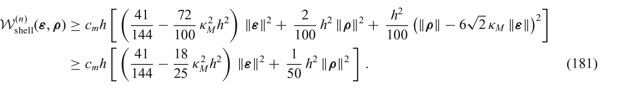
Using relation (172) in equation (170), we deduce that inequality (169) is true. Then, substituting relation (169) into equation (168), we obtain the estimate

$${\mathcal{W}}_{\mathrm{shell}}^{(2m+1)}(\mathit{\epsilon },\mathit{\rho })\ge \frac{41}{144}h{W}_s(\mathit{\epsilon })+[\frac{h^3}{30}+\sum _{k=2}^m(c_{2k-2}-\frac{c_{2k-3}^2}{c_{2k-4}})I_{2k+1}]W_s(\mathit{\rho }-2\mathit{\epsilon }\mathit{\kappa }),$$

(173)

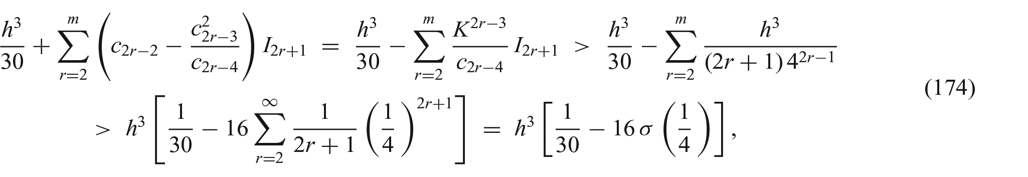
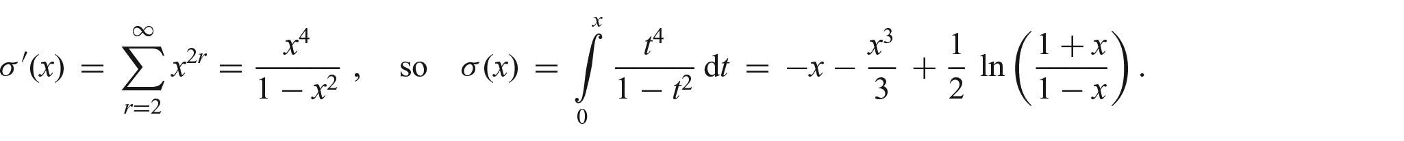
which holds for any $m\ge 2$ . Next, we want to show that the above expression in brackets is bounded from below by a positive constant. Applying now Lemma 5 (ii) and (iii), we can write successively

$$\begin{array}{c}\frac{h^3}{30}+\sum _{r=2}^m(c_{2r-2}-\frac{c_{2r-3}^2}{c_{2r-4}})I_{2r+1}=\frac{h^3}{30}-\sum _{r=2}^m\frac{K^{2r-3}}{c_{2r-4}}{I}_{2r+1}>\frac{h^3}{30}-\sum _{r=2}^m\frac{h^3}{(2r+1)4^{2r-1}}\hfill \\ \multicolumn{1}{c}{>h^3[\frac{1}{30}-16\sum _{r=2}^{\infty }\frac{1}{2r+1}{\left(\frac{1}{4}\right)}^{2r+1}]=h^3[\frac{1}{30}-16\sigma \left(\frac{1}{4}\right)],}\end{array}$$

(174)

where we have denoted by $\sigma (x)$ the function

$$\sigma (x):=\sum _{r=2}^{\infty }\frac{x^{2r+1}}{2r+1}\mathrm{for}\mathrm{any}x\in (0,1).$$

(175)

Then, we get

$${\sigma }^{\prime }(x)=\sum _{r=2}^{\infty }{x}^{2r}=\frac{x^4}{1-x^2},\mathrm{so}\sigma (x)=\underset{0}{\overset{x}{\int }}\frac{t^4}{1-t^2}\mathrm{d}t=-x-\frac{x^3}{3}+\frac{1}{2}\ln \left(\frac{1+x}{1-x}\right).$$

For $x=\frac{1}{4}$ we compute

$$\sigma \left(\frac{1}{4}\right)=-\frac{1}{4}-\frac{1}{192}+\frac{1}{2}\ln \frac{5}{3}$$

and inserting into equation (174) we deduce

$$\frac{h^3}{30}+\sum _{r=2}^m(c_{2r-2}-\frac{c_{2r-3}^2}{c_{2r-4}})I_{2r+1}>h^3(\frac{1}{30}+4+\frac{1}{12}-8\ln \frac{5}{3})>h^3·0.03.$$

(176)

Thus, we derive from equations (173) and (176) that

$${\mathcal{W}}_{\mathrm{shell}}^{(2m+1)}(\mathit{\epsilon },\mathit{\rho })\ge \frac{41}{144}h{W}_s(\mathit{\epsilon })+\frac{3}{100}{h}^3{W}_s(\mathit{\rho }-2\mathit{\epsilon }\mathit{\kappa }),$$

(177)

and using inequality (133) we get

$${\mathcal{W}}_{\mathrm{shell}}^{(2m+1)}(\mathit{\epsilon },\mathit{\rho })\ge c_{m}h[\frac{41}{144}\parallel \mathit{\epsilon }{\parallel }^2+\frac{3}{100}{h}^2\parallel \mathit{\rho }-2\mathrm{sym}(\mathit{\epsilon }\mathit{\kappa }){\parallel }^2].$$

(178)

To estimate the last term we write

$$\parallel \mathit{\rho }-2\mathrm{sym}(\mathit{\epsilon }\mathit{\kappa }){\parallel }^2=\parallel \mathit{\rho }{\parallel }^2-4\mathit{\rho }·(\mathit{\epsilon }\mathit{\kappa })+4\parallel \mathrm{sym}(\mathit{\epsilon }\mathit{\kappa }){\parallel }^2\ge \parallel \mathit{\rho }{\parallel }^2-4\mathit{\epsilon }·(\mathit{\rho }\mathit{\kappa })\ge \parallel \mathit{\rho }{\parallel }^2-4\parallel \mathit{\epsilon }\parallel ·\parallel \mathit{\rho }\mathit{\kappa }\parallel$$

(179)

and

$$\begin{array}{c}\parallel \mathit{\rho }\mathit{\kappa }{\parallel }^2=\parallel \mathit{\rho }({\kappa }_1{\mathit{u}}_1\otimes {\mathit{u}}_1+{\kappa }_2{\mathit{u}}_2\otimes {\mathit{u}}_2){\parallel }^2\le 2{\kappa }_1^2\parallel \mathit{\rho }{\mathit{u}}_1\otimes {\mathit{u}}_1{\parallel }^2+2{\kappa }_2^2\parallel \mathit{\rho }{\mathit{u}}_2\otimes {\mathit{u}}_2{\parallel }^2\hfill \\ \le 2{\kappa }_M^2(\parallel \mathit{\rho }{\mathit{u}}_1\otimes {\mathit{u}}_1{\parallel }^2+\parallel \mathit{\rho }{\mathit{u}}_2\otimes {\mathit{u}}_2{\parallel }^2)=2{\kappa }_M^2\parallel \mathit{\rho }{\parallel }^2,\hfill \end{array}$$

(180)

in view of equation (153). Then, using equations (179) and (180) in equation (178), we infer

$${\mathcal{W}}_{\mathrm{shell}}^{(2m+1)}(\mathit{\epsilon },\mathit{\rho })\ge c_{m}h[\frac{41}{144}\parallel \mathit{\epsilon }{\parallel }^2+\frac{3}{100}{h}^2(\parallel \mathit{\rho }{\parallel }^2-4\sqrt{2}{\kappa }_M\parallel \mathit{\epsilon }\parallel ·\parallel \mathit{\rho }\parallel )].$$

Hence, for any $n=2m+1\ge 5$ we have

$$\begin{array}{c}{\mathcal{W}}_{\mathrm{shell}}^{(n)}(\mathit{\epsilon },\mathit{\rho })\ge c_{m}h[(\frac{41}{144}-\frac{72}{100}{\kappa }_M^2{h}^2)\parallel \mathit{\epsilon }{\parallel }^2+\frac{2}{100}{h}^2\parallel \mathit{\rho }{\parallel }^2+\frac{h^2}{100}{(\parallel \mathit{\rho }\parallel -6\sqrt{2}{\kappa }_M\parallel \mathit{\epsilon }\parallel )}^2]\hfill \\ \ge c_{m}h[(\frac{41}{144}-\frac{18}{25}{\kappa }_M^2{h}^2)\parallel \mathit{\epsilon }{\parallel }^2+\frac{1}{50}{h}^2\parallel \mathit{\rho }{\parallel }^2].\hfill \end{array}$$

(181)

In view of ${\kappa }_{M}h<\frac{1}{2}$ , we have

$$\frac{41}{144}-\frac{18}{25}{\kappa }_M^2{h}^2>\frac{41}{144}-\frac{18}{25}·\frac{1}{4}=\frac{377}{3600}>\frac{1}{10}.$$

Using this inequality in equation (181), we get

$${\mathcal{W}}_{\mathrm{shell}}^{(n)}(\mathit{\epsilon },\mathit{\rho })\ge c_{m}h(\frac{1}{10}\parallel \mathit{\epsilon }{\parallel }^2+\frac{1}{50}{h}^2\parallel \mathit{\rho }{\parallel }^2),$$

i.e., the coercivity relation (165) holds. The proof is complete. ■

5.3. Coercivity result for the shell model of order $O(h^3)$

In the case $n=3$ , the expression of the strain energy density is given by equation (129), or equivalently (130). We notice that the energy function has a special form (since the higher order terms do not appear) and we need to proceed in a different manner to prove the coercivity.

Let us denote by $r$ the ratio between $c_m$ and $c_M$ , i.e.,

$$r:=\frac{c_m}{c_M}\in (0,1],$$

(182)

where $c_m$ and $c_M$ are defined by equation (132). Note that we can also write

$$r=min\{\frac{\lambda +2\mu }{3\lambda +2\mu },\frac{3\lambda +2\mu }{\lambda +2\mu }\}={\left(\frac{\lambda +2\mu }{3\lambda +2\mu }\right)}^{\mathrm{sgn}(\lambda )},$$

(183)

since we have

$$\frac{\lambda +2\mu }{3\lambda +2\mu }\le 1\le \frac{3\lambda +2\mu }{\lambda +2\mu }\mathrm{if}\lambda \ge 0,$$

and conversely

$$\frac{3\lambda +2\mu }{\lambda +2\mu }<1<\frac{\lambda +2\mu }{3\lambda +2\mu }\mathrm{if}\lambda <0.$$

We can formulate now the coercivity result.

Proposition 7. Assume that the principal curvatures ${\kappa }_{\alpha }$ of the reference midsurface are such that

$$|{\kappa }_{\alpha }|h<\frac{1}{2}r=\frac{1}{2}min\{\frac{\lambda +2\mu }{3\lambda +2\mu },\frac{3\lambda +2\mu }{\lambda +2\mu }\}.$$

(184)

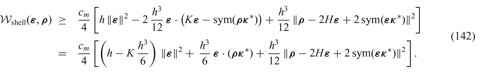
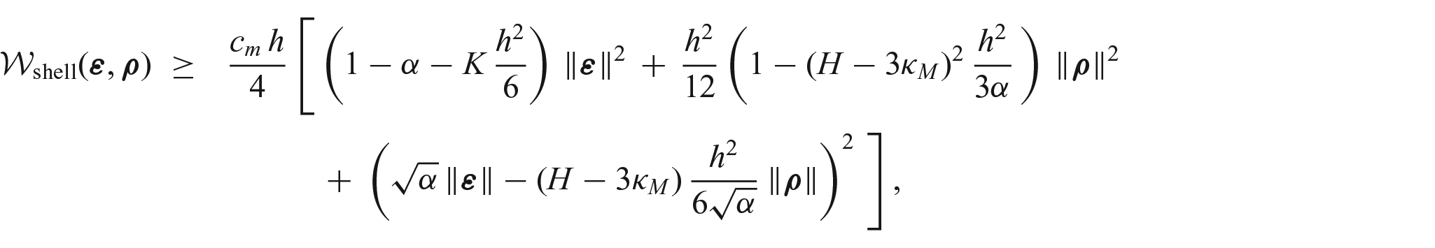
Then, the strain energy density function for the shell model of order $O(h^3)$ given by equation (130)satisfies the following coercivity inequality:

$${\mathcal{W}}_{\mathrm{shell}}^{(3)}(\mathit{\epsilon },\mathit{\rho })\ge \frac{c_{m}h}{12}(\frac{1}{4}\parallel \mathit{\epsilon }{\parallel }^2+\frac{2}{5}{h}^2\parallel \mathit{\rho }{\parallel }^2).$$

(185)

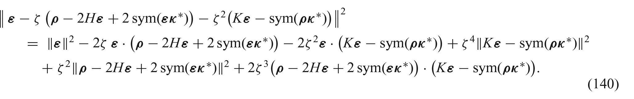
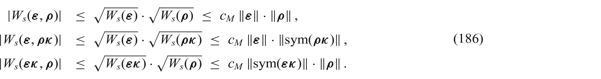
Proof. For the coupling terms in the energy function (130), we can use the Cauchy–Schwarz inequality and relation (133) to estimate

$$\begin{array}{c}|W_s(\mathit{\epsilon },\mathit{\rho })|\le \sqrt{W_s(\mathit{\epsilon })}·\sqrt{W_s(\mathit{\rho })}\le c_M\parallel \mathit{\epsilon }\parallel ·\parallel \mathit{\rho }\parallel ,\hfill \\ \multicolumn{1}{c}{|W_s(\mathit{\epsilon },\mathit{\rho }\mathit{\kappa })|\le \sqrt{W_s(\mathit{\epsilon })}·\sqrt{W_s(\mathit{\rho }\mathit{\kappa })}\le c_M\parallel \mathit{\epsilon }\parallel ·\parallel \mathrm{sym}(\mathit{\rho }\mathit{\kappa })\parallel ,}\\ \multicolumn{1}{c}{|W_s(\mathit{\epsilon }\mathit{\kappa },\mathit{\rho })|\le \sqrt{W_s(\mathit{\epsilon }\mathit{\kappa })}·\sqrt{W_s(\mathit{\rho })}\le c_M\parallel \mathrm{sym}(\mathit{\epsilon }\mathit{\kappa })\parallel ·\parallel \mathit{\rho }\parallel .}\end{array}$$

(186)

Moreover, for the norms $\parallel \mathrm{sym}(\mathit{\epsilon }\mathit{\kappa })\parallel$ and $\parallel \mathrm{sym}(\mathit{\rho }\mathit{\kappa })\parallel$ , we have the inequalities

$$\parallel \mathrm{sym}(\mathit{\epsilon }\mathit{\kappa })\parallel \le {\kappa }_M\parallel \mathit{\epsilon }\parallel \mathrm{and}\parallel \mathrm{sym}(\mathit{\rho }\mathit{\kappa })\parallel \le {\kappa }_M\parallel \mathit{\rho }\parallel ,$$

(187)

which can be justified as follows: for any symmetric tensor $\mathit{\phi }={\phi }_{\alpha \beta }{\mathit{u}}_{\alpha }\otimes {\mathit{u}}_{\beta }$ , we have

$$\mathit{\phi }\mathit{\kappa }=({\phi }_{\alpha \beta }{\mathit{u}}_{\alpha }\otimes {\mathit{u}}_{\beta })({\kappa }_1{\mathit{u}}_1\otimes {\mathit{u}}_1+{\kappa }_2{\mathit{u}}_2\otimes {\mathit{u}}_2)={\kappa }_1{\phi }_{\alpha 1}{\mathit{u}}_{\alpha }\otimes {\mathit{u}}_1+{\kappa }_2{\phi }_{\alpha 2}{\mathit{u}}_{\alpha }\otimes {\mathit{u}}_2.$$

Then, the symmetric part is

$$\mathrm{sym}(\mathit{\phi }\mathit{\kappa })={\kappa }_1{\phi }_{11}{\mathit{u}}_1\otimes {\mathit{u}}_1+\frac{{\kappa }_1+{\kappa }_2}{2}{\phi }_{12}({\mathit{u}}_1\otimes {\mathit{u}}_2+{\mathit{u}}_2\otimes {\mathit{u}}_1)+{\kappa }_2{\phi }_{22}{\mathit{u}}_2\otimes {\mathit{u}}_2$$

and, hence,

$$\parallel \mathrm{sym}(\mathit{\phi }\mathit{\kappa }){\parallel }^2={\kappa }_1^2{\phi }_{11}^2+{\kappa }_2^2{\phi }_{22}^2+\frac{1}{2}({\kappa }_1+{\kappa }_2{)}^2{\phi }_{12}^2\le {\kappa }_M^2({\phi }_{11}^2+{\phi }_{22}^2+2{\phi }_{12}^2)={\kappa }_M^2\parallel \mathit{\phi }{\parallel }^2.$$

Thus, relations (187) hold true.

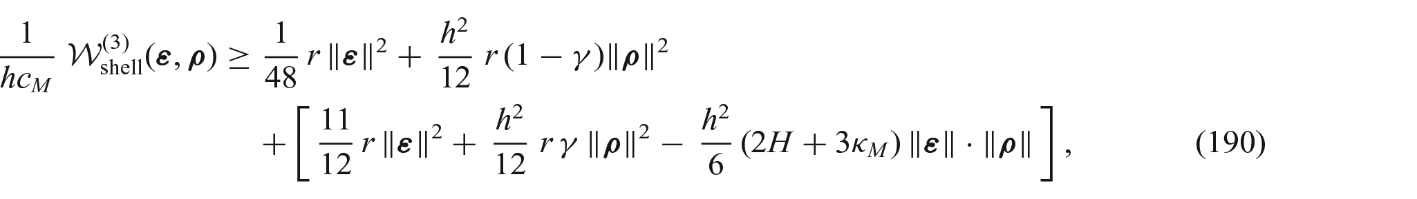
Making use of inequalities (133), (186), and (187) in the expression of the energy (130), we derive that

$${\mathcal{W}}_{\mathrm{shell}}^{(3)}(\mathit{\epsilon },\mathit{\rho })\ge (h-K\frac{h^3}{4})c_m\parallel \mathit{\epsilon }{\parallel }^2+\frac{h^3}{12}{c}_m\parallel \mathit{\rho }{\parallel }^2-H\frac{h^3}{3}{c}_M\parallel \mathit{\epsilon }\parallel ·\parallel \mathit{\rho }\parallel -\frac{h^3}{2}{c}_M{\kappa }_M\parallel \mathit{\epsilon }\parallel ·\parallel \mathit{\rho }\parallel ,$$

or equivalently, dividing by $h{c}_M$ and using notation (182),

$$\frac{1}{h{c}_M}{\mathcal{W}}_{\mathrm{shell}}^{(3)}(\mathit{\epsilon },\mathit{\rho })\ge (1-K\frac{h^2}{4})r\parallel \mathit{\epsilon }{\parallel }^2+\frac{h^2}{12}r\parallel \mathit{\rho }{\parallel }^2-\frac{h^2}{6}(2H+3{\kappa }_M)\parallel \mathit{\epsilon }\parallel ·\parallel \mathit{\rho }\parallel ,$$

(188)

Since $|{\kappa }_{\alpha }|h<\frac{1}{2}r\le \frac{1}{2}$ by hypothesis, the coefficient of $\parallel \mathit{\epsilon }{\parallel }^2$ can be decomposed as follows:

$$1-K\frac{h^2}{4}\ge 1-\frac{|{\kappa }_{1}h|·|{\kappa }_{2}h|}{4}>1-\frac{1}{16}=\frac{15}{16}=\frac{1}{48}+\frac{11}{12}.$$

(189)

Using relation (189) in equation (188), we can write

$$\begin{array}{c}\frac{1}{h{c}_M}{\mathcal{W}}_{\mathrm{shell}}^{(3)}(\mathit{\epsilon },\mathit{\rho })\ge \frac{1}{48}r\parallel \mathit{\epsilon }{\parallel }^2+\frac{h^2}{12}r(1-\gamma )\parallel \mathit{\rho }{\parallel }^2\hfill \\ +[\frac{11}{12}r\parallel \mathit{\epsilon }{\parallel }^2+\frac{h^2}{12}r\gamma \parallel \mathit{\rho }{\parallel }^2-\frac{h^2}{6}(2H+3{\kappa }_M)\parallel \mathit{\epsilon }\parallel ·\parallel \mathit{\rho }\parallel ],\hfill \end{array}$$

(190)

where $\gamma \in (0,1)$ is a constant which will be precised later on. Notice that the function in the square brackets in relation (190) is a quadratic form in the variables $\parallel \mathit{\epsilon }\parallel$ , $\parallel \mathit{\rho }\parallel$ . This function is always positive, provided that its discriminant $\mathrm{\Delta }$ is negative. Let us compute the discriminant

$$\mathrm{\Delta }=\frac{h^4}{36}(2H+3{\kappa }_M{)}^2-\frac{11}{3}·\frac{h^2}{12}{r}^2\gamma =\frac{h^2}{36}[h^2(2H+3{\kappa }_M{)}^2-11r^2\gamma ].$$

(191)

In view of the hypothesis (184), we have $|\mathrm{Hh}|<\frac{1}{2}r$ and ${\kappa }_{M}h<\frac{1}{2}r$ , so

$$h^2(2H+3{\kappa }_M{)}^2\le (2|\mathrm{Hh}|+3{\kappa }_{M}h{)}^2<{(r+\frac{3}{2}r)}^2=\frac{25}{4}{r}^2.$$

(192)

From equations (191) and (192), it follows that

$$\mathrm{\Delta }<\frac{h^2}{36}[\frac{25}{4}{r}^2-11r^2\gamma ]=\frac{11}{36}{h}^2{r}^2[\frac{25}{44}-\gamma ].$$

(193)

Since $\frac{25}{44}=0.568\dots$ , we choose now $\gamma =0.6$ and relation (193) shows that $\mathrm{\Delta }<0$ . Hence, the function in square brackets in equation (190) is always positive (for $\gamma =0.6$ ) and thus we derive

$$\frac{1}{h{c}_M}{\mathcal{W}}_{\mathrm{shell}}^{(3)}(\mathit{\epsilon },\mathit{\rho })\ge \frac{1}{48}r\parallel \mathit{\epsilon }{\parallel }^2+\frac{h^2}{12}·\frac{4}{10}r\parallel \mathit{\rho }{\parallel }^2,$$

which is equivalent to the coercivity relation (185). This completes the proof. ■

Remark: Since the strain energy density ${\mathcal{W}}_{\mathrm{shell}}^{(n)}(\mathit{\epsilon },\mathit{\rho })$ is coercive (for all $n\ge 3$ ), one can use the Korn inequality for surfaces and the Lax–Milgram theorem as in the classical linear theory [19, 20, 22] to show the existence of weak solutions for the equilibrium equations of shells.

In the dynamical case, one can employ these results in conjunction with the theory of semigroups of operators to prove the existence of solutions to the equations of motion (see the work by Bîrsan [23] for the case of Cosserat shells).

6. Conclusion

In this paper, we have obtained by dimensional reduction a general expression of the areal strain energy density for linear elastic shells. Using usual shell assumptions and approximations, we have derived the reduced explicit form of the energy function, in which the coefficients are expressed as integrals depending on the thickness $h$ and curvatures $H,K$ . By developing these coefficients as power series of $h$ , and truncating the series at the power $h^n$ , we have deduced the constitutive shell model of order $O(h^n)$ . Finally, we have showed that the proposed areal strain energy functions (both for finite $n\ge 3$ and for $n\to \infty$ ) are coercive. This property is a decisive step in the proof of existence of minimizers for the shell energy.