Asymptotic theory for the inextensional flexure and twist of plastically deformed thin rods

Abstract

A concise derivation of Kirchhoff’s theory for naturally curved and twisted rods is presented as a prelude to the derivation of the theory for the elastic response of rods that have undergone prior plastic deformation.

1. Introduction

The purpose of this note is to extend the theory of thin elastic rods to accommodate prior plastic deformation. To aid in this endeavor, we first outline the theory for purely elastic deformations of rods that are naturally curved and twisted. The presence of plastic deformation is taken into account for initially straight and untwisted rods, and a set of restrictions on the plastic deformation which are such as to render this theory equivalent to the first theory are given. In this way, we exhibit the manner in which a rod may acquire a natural shape by being subjected to plastic deformation.

Our approach entails a “dimension reduction” from three-dimensional theory, in contrast to the direct approach in which the rod is regarded as a curve endowed a priori with particular kinematical and dynamical structures [1–3]. Derivations based on three-dimensional elasticity are the subject of a voluminous literature [1–11]. The older work in this area is ably summarized, assessed, and interpreted by Dill [12], with more recent efforts culminating in the rigorous derivation, by Mora and Müller [13], of Kirchhoff’s theory for naturally straight, untwisted rods. In a major reinvigoration of the field, Goriely [14] and Kaczmarski et al. [15] have recently extended this theory to accommodate growth mechanics.

The advanced state of the literature concerned with the derivation of the theory suggests that little is to be gained by adding to it. However, our view is that a concise, pedagogically useful treatment, suitable for students of Mechanics, is lacking. To address this, we draw on [12] and [13], but work at a level of rigor intermediate between the two. Concerning notation, we use $\mathrm{Sym}\mathit{A}$ and $\mathrm{Skw}\mathit{A}$ , respectively, to denote the symmetric and skew parts of a second-order tensor $\mathit{A}$ , and $\mathrm{ax}(\mathrm{Skw}\mathit{A})$ to denote the axial vector of $\mathrm{Skw}\mathit{A}$ , defined by $\mathrm{ax}(\mathrm{Skw}\mathit{A})\times \mathbf{\upsilon }=(\mathrm{Skw}\mathit{A})\mathbf{\upsilon }$ for any vector $\mathbf{\upsilon }$ . The group of rotation tensors is denoted by $\mathrm{Ort}{h}^{+}.$ The tensor product of three-vectors is indicated by interposing the symbol ⊗, and the Euclidean inner product of tensors $\mathit{A},\mathit{B}$ is denoted and defined by $\mathit{A}·\mathit{B}=\mathrm{tr}(\mathit{A}{\mathit{B}}^t)$ , where the superscript ^t stands for transpose and $\mathrm{tr}(·)$ is the trace; the induced norm is $\left|\mathit{A}\right|=\sqrt{\mathit{A}·\mathit{A}}$ . The symbol |·| is also used to denote the usual Euclidean norm of three-vectors. If $\mathit{A}$ is invertible, its cofactor is ${\mathit{A}}^{*}=(det\mathit{A}){\mathit{A}}^{-t}$ , where $\det (·)$ is the determinant. We use $\mathcal{C}[\mathit{A}]$ to denote the linear action of the fourth-order tensor $\mathcal{C}$ on a second-order tensor. This has Cartesian components ${\mathcal{C}}_{\mathrm{ijkl}}{A}_{\mathrm{kl}}$ . A bold subscript attached to a scalar is used to denote its tensor-valued derivative with respect to the indicated tensor variable. Finally, Latin and Greek indices take values in $\{1,2,3\}$ and $\{1,2\}$ , respectively, and, when repeated, are summed over their ranges.

We discuss the kinematics of inextensional deformations of rods in section 2. In section 3, the energy of Kirchhoff’s theory is shown to furnish the leading-order strain-energy function for naturally curved and twisted thin rods composed of a uniform simple elastic solid. We conclude, in section 4, with a discussion of the theory extended to account for prior plastic deformation.

2. Deformations of naturally curved and twisted rods

The position of a material point in a fixed reference configuration $\kappa$ is described by Dill [12]:

$$\mathit{X}=\mathit{x}(S)+X_{\alpha }{\mathit{E}}_{\alpha }(S),$$

(1)

where $\mathit{x}(S)$ is the parametric representation of the curve $c$ of centroids of the cross-sections of the rod in terms of arclength $S$ ; $X_{\alpha }$ are the Cartesian coordinates in a cross-sectional plane $\mathrm{\Omega }$ defined by $S=\mathrm{const}.$ and spanned by $\{{\mathit{E}}_{\alpha }\}$ ; and $\{{\mathit{E}}_{\alpha },{\mathit{E}}_3\},$ with ${\mathit{E}}_3(S)={\mathit{x}}^{\prime }(S)$ , is a right-handed orthonormal basis at each $S\in [0,l]$ . Here, $l$ is the total arclength of the rod, and $(·{)}^{\prime }=\partial (·)/\partial S$ at fixed $X_{\alpha }$ . We assume $\mathrm{\Omega }$ to be simply connected and that its centroid $X_{\alpha }=0$ is contained in $\mathrm{\Omega }$ . Generalizations to account for thin-walled open or closed cross-sections are discussed in Villaggio [1] and Dill [16]. We further suppose $\partial \mathrm{\Omega }$ to be the curve defined by an equation of the form $f(X_1,X_2)=0$ , and thus, that the shape and dimensions of the cross-section are independent of $S$ .

Let $h$ be the diameter of $\mathrm{\Omega }$ . We consider rods that are thin in the sense that $h/l<<1$ . Taking $l$ as the unit of length $(l=1)$ , we thus have $h<<1$ , and we seek a model for rods valid to leading order in $h$ . To this end, it proves convenient to introduce scaled coordinates $Z_{\alpha }=O(1)$ defined by:

$$h{Z}_{\alpha }=X_{\alpha },$$

(2)

and to express equation (1) as:

$$\mathit{X}(Z_{\alpha },S)=\mathit{x}(S)+h{Z}_{\alpha }{\mathit{E}}_{\alpha }(S).$$

(3)

After deformation the material point $\mathit{X}$ moves to the position $\mathit{\chi }(\mathit{X})$ . We write this in the form:

$$\mathit{\chi }(\mathit{X}(Z_{\mathbf{\alpha }},S))=\mathit{r}(S)+h{Z}_{\alpha }{\mathit{d}}_{\alpha }(S)+h^2\mathit{u}(Z_{\alpha },S;h),$$

(4)

where $\mathit{u}$ and its coordinate derivatives are assumed to be regular functions of $h$ , where:

$$\mathit{r}(S)=\mathit{\chi }(\mathit{x}(S)),$$

(5)

is the parametric equation of the image in the deformed configuration of the initial curve of centroids, and where:

$${\mathit{d}}_{\alpha }(S)=\frac{\partial }{\partial X_{\alpha }}{\mathit{\chi }}_{|c}.$$

(6)

Accordingly, we require that:

$${\mathit{u}}_{|c}=0\mathrm{and}{\mathit{u}}_{,\alpha |c}=0,$$

(7)

where $(·{)}_{,\alpha }=\partial (·)/\partial Z_{\alpha }$ .

The representation (4) may be motivated by a Taylor expansion of $\mathit{\chi }$ about the centroidal curve $c.$ For example, if $\mathit{\chi }$ is twice differentiable with respect to the $X_{\mathbf{\alpha }}$ , then:

$$\mathit{u}(Z_{\alpha },S;h)=\frac{1}{2}{Z}_{\alpha }{Z}_{\beta }{\mathit{g}}_{\alpha \beta }(S)+\frac{\mathit{o}(h^2)}{h^2},\mathrm{where}{\mathit{g}}_{\alpha \beta }=\frac{{\partial }^2}{\partial X_{\alpha }\partial X_{\beta }}{\mathit{\chi }}_{|c},$$

(8)

and $|\mathit{o}(h^2)|=o(h^2)$ . However, in view of Dill’s remarks [12] to the effect that equation (8) is overly restrictive, we work directly with equation (4), regarded as the definition of $\mathit{u}$ in terms of $\mathit{\chi }(\mathit{X})$ .

An expression for the deformation gradient $\mathit{F}$ is obtained via the chain rule in the form:

$$d\mathit{\chi }=\mathit{F}d\mathit{X},$$

(9)

where:

$$d\mathit{X}=({\mathit{E}}_3+h{Z}_{\alpha }{\mathit{E}}_{\alpha }^{\prime })\mathrm{dS}+h{\mathit{E}}_{\alpha }d{Z}_{\alpha },$$

(10)

and

$$d\mathit{\chi }=({\mathit{r}}^{\prime }+h{Z}_{\alpha }{\mathit{d}}_{\alpha }^{\prime }+h^2{\mathit{u}}^{\prime })\mathrm{dS}+(h{\mathit{d}}_{\alpha }+h^2{\mathit{u}}_{,\alpha })d{Z}_{\alpha }.$$

(11)

Let $\{{\mathit{D}}_i\}$ be a fixed right-handed orthonormal background frame. Then,

$$\mathit{A}(S)={\mathit{E}}_i(S)\otimes {\mathit{D}}_i,$$

(12)

is a rotation field, and,

$${\mathit{E}}_{\alpha }^{\prime }=\overline{\kappa }\times {\mathit{E}}_{\alpha },\mathrm{where}\overline{\kappa }=\mathrm{ax}({\mathit{A}}^{\prime }{\mathit{A}}^t).$$

(13)

Accordingly, from equation (10),

$${\mathit{E}}_3·d\mathit{X}=(1+h{\mathit{E}}_3·\overline{\kappa }\times \mathit{Z})\mathrm{dS}\mathrm{and}{\mathit{E}}_{\beta }·d\mathit{X}=h({\mathit{E}}_{\beta }·\overline{\kappa }\times \mathit{Z}\mathrm{dS}+d{Z}_{\beta }),$$

(14)

where:

$$\mathit{Z}=Z_{\alpha }{\mathit{E}}_{\alpha }.$$

(15)

For small $h$ , we then have:

$$\mathrm{dS}=[1-h{\mathit{E}}_3·\overline{\kappa }\times \mathit{Z}+o(h)]{\mathit{E}}_3·d\mathit{X}\mathrm{and}d{Z}_{\beta }=[h^{-1}{\mathit{E}}_{\beta }-({\mathit{E}}_{\beta }·\overline{\kappa }\times \mathit{Z}){\mathit{E}}_3+\mathit{O}(h)]·d\mathit{X},$$

(16)

where $|\mathit{O}(h)|=O(h),$ which we combine with equations (9) and (11) to derive:

$$\mathit{F}=\{{\mathit{r}}^{\prime }+h[Z_{\alpha }{\mathit{d}}_{\alpha }^{\prime }-({\mathit{E}}_3·\overline{\kappa }\times \mathit{Z}){\mathit{r}}^{\prime }-({\mathit{E}}_{\alpha }·\overline{\kappa }\times \mathit{Z}){\mathit{d}}_{\alpha }]\}\otimes {\mathit{E}}_3+({\mathit{d}}_{\alpha }+h{\mathit{u}}_{,\alpha })\otimes {\mathit{E}}_{\alpha }+\mathit{o}(h),$$

(17)

where $|\mathit{o}(h)|=o(h)$ .

We are concerned with deformations that induce inextensional bending and twisting of the rod at the curve of centroids, and thus impose the restriction:

$${\mathit{F}}_{|c}=\mathit{R}(S)\in \mathrm{Ort}{h}^{+}.$$

(18)

From equations (7)₂ and (17), we then have that:

$${\mathit{r}}^{\prime }\otimes {\mathit{E}}_3+{\mathit{d}}_{\alpha }\otimes {\mathit{E}}_{\alpha }=\mathit{R}+\mathit{o}(h),$$

(19)

yielding:

$$\{{\mathit{d}}_{\alpha },{\mathit{r}}^{\prime }\}=\{{\mathit{e}}_{\alpha },{\mathit{e}}_3\}+\mathit{o}(h),$$

(20)

with:

$${\mathit{e}}_i(S)=\mathit{R}{\mathit{E}}_i.$$

(21)

Here, ${\mathit{e}}_3$ is a field of unit tangents to the deformed centroidal curve. We note that $\{{\mathit{e}}_i\}$ , like $\{{\mathit{E}}_i\}$ , is a right-handed orthonormal basis at every $S\in [0,l]$ .

Equations (12), (13), and (21) furnish:

$${\mathit{e}}_i^{\prime }=\mathit{R}({\mathit{R}}^t{\mathit{R}}^{\prime }{\mathit{E}}_i+\overline{\kappa }\times {\mathit{E}}_i)=\mathit{R}[(\mathit{\gamma }+\overline{\kappa })\times {\mathit{E}}_i],$$

(22)

where:

$$\mathit{\gamma }=\mathrm{ax}({\mathit{R}}^t{\mathit{R}}^{\prime }),$$

(23)

is the flexure-twist strain of the centroidal curve, and we note that: ¹

$$\mathit{\gamma }=\kappa -\overline{\kappa },\mathrm{where}\kappa ={\mathit{R}}^t\mathit{\omega },$$

(24)

in which $\mathit{\omega }(S)$ is the vector field such that ${\mathit{e}}_i^{\prime }=\mathit{\omega }\times {\mathit{e}}_i$ .

On combining equations (20) and (22) with:

$$({\mathit{E}}_3·\overline{\kappa }\times \mathit{Z}){\mathit{E}}_3+({\mathit{E}}_{\alpha }·\overline{\kappa }\times \mathit{Z}){\mathit{E}}_{\alpha }=\overline{\kappa }\times \mathit{Z},$$

(25)

we reduce equation (17) to:

$$\mathit{F}=\mathit{R}(\mathit{I}+\mathit{E}),$$

(26)

where $\mathit{I}={\mathit{E}}_i\otimes {\mathit{E}}_i$ is the identity for three-space, and:

$$\mathit{E}=h[\mathit{\gamma }\times \mathit{Z}\otimes {\mathit{E}}_3+{({\mathit{R}}^t\mathit{u})}_{,\alpha }\otimes {\mathit{E}}_{\alpha }]+\mathit{o}(h).$$

(27)

3. Elastic energy of naturally curved and twisted rods

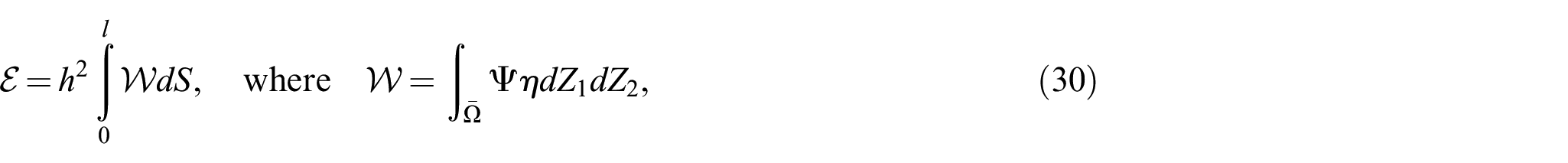
We assume the underlying three-dimensional continuum to be a uniform elastic material characterized by a function $\mathrm{\Psi }(\mathit{F})$ representing strain energy per unit reference volume. The total strain energy stored in the rod is:

$$\mathcal{E}={\int }_{\kappa }\mathrm{\Psi }\mathrm{dV},$$

(28)

with:

$$\mathrm{dV}=(\frac{\partial \mathit{X}}{\partial X_1}\times \frac{\partial \mathit{X}}{\partial X_2}·\frac{\partial \mathit{X}}{\partial S})d{X}_{1}d{X}_2\mathrm{dS}=h^2\eta d{Z}_{1}d{Z}_2\mathrm{dS},\mathrm{where}\eta =1+h{\mathit{E}}_3·\overline{\kappa }\times \mathit{Z}.$$

(29)

Thus,

$$\mathcal{E}=h^2\underset{0}{\overset{l}{\int }}\mathcal{W}\mathrm{dS},\mathrm{where}\mathcal{W}={\int }_{\overline{\mathrm{\Omega }}}\mathrm{\Psi }\eta d{Z}_{1}d{Z}_2,$$

(30)

and where $\overline{\mathrm{\Omega }}$ is the image of $\mathrm{\Omega }$ in the $Z_1,Z_2$ plane.

3.1. Constitutive hypotheses and the leading-order energy for thin rods

We assume that $\mathrm{\Psi }(\mathit{F})=\mathrm{\Psi }(\mathit{QF})$ for arbitrary rotations $\mathit{Q}$ . As is well known [17,18], this is the necessary and sufficient condition for the symmetry of the associated Cauchy stress $\mathit{T}$ defined by ${\mathrm{\Psi }}_{\mathit{F}}=\mathit{T}{\mathit{F}}^{*}$ . We further suppose that $\mathrm{\Psi }(\mathit{I})=0$ and ${\mathrm{\Psi }}_{\mathit{F}}(\mathit{I})=0$ , so that the energy and stress vanish when the body is undeformed. In these circumstances, we have ${\mathrm{\Psi }}_{\mathit{FF}}(\mathit{I})[\mathit{A}]=\mathcal{C}[\mathit{A}]$ (see [18], equation (11.5)) for any tensor $\mathit{A}$ , where $\mathcal{C}$ is the classical fourth-order tensor of elastic moduli possessing the major symmetry $\mathcal{C}={\mathcal{C}}^t$ , with ${\mathcal{C}}^t$ defined by $\mathit{A}·\mathcal{C}[\mathit{B}]=\mathit{B}·{\mathcal{C}}^t[\mathit{A}]$ , together with the minor symmetries ${\mathit{A}}^t·\mathcal{C}[\mathit{B}]=\mathit{A}·\mathcal{C}[\mathit{B}]$ and $\mathit{A}·\mathcal{C}[{\mathit{B}}^t]=\mathit{A}·\mathcal{C}[\mathit{B}]$ . We assume this to be positive definite in the sense that $\mathit{A}·\mathcal{C}[\mathit{A}]>0$ for all non-zero symmetric $\mathit{A}$ . It then follows from the minor symmetries that $\mathit{A}·\mathcal{C}[\mathit{A}]\ge 0$ for all $\mathit{A}$ . For example, in the case of isotropic symmetry relative to $\kappa$ , we have:

$$\mathcal{C}[\mathit{A}]=\lambda (\mathrm{tr}\mathit{A})\mathit{I}+2\mu \mathrm{Sym}\mathit{A},$$

(31)

where $\lambda$ and $\mu$ , with $\mu >0$ and $3\lambda +2\mu >0$ , are the Lamé moduli.

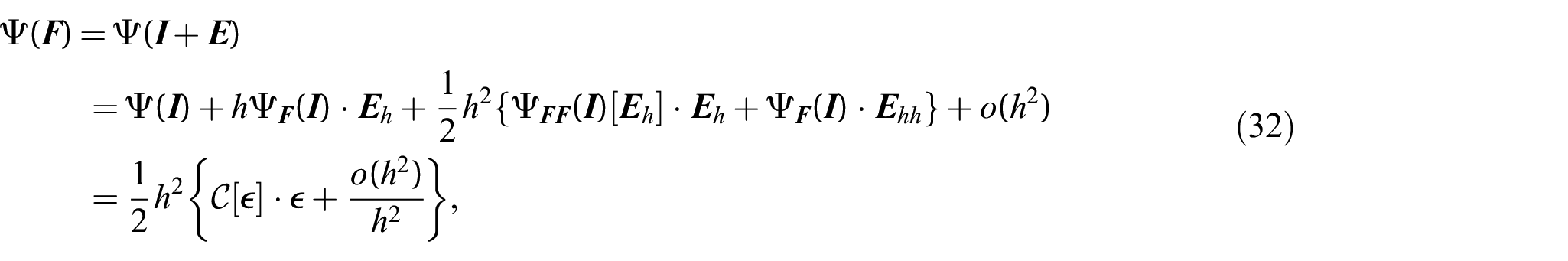
Our constitutive hypotheses, together with equations (26) and (27), imply that:

$$\begin{array}{c}\mathrm{\Psi }(\mathit{F})=\mathrm{\Psi }(\mathit{I}+\mathit{E})\hfill \\ =\mathrm{\Psi }(\mathit{I})+h{\mathrm{\Psi }}_{\mathit{F}}(\mathit{I})·{\mathit{E}}_h+\frac{1}{2}{h}^2\{{\mathrm{\Psi }}_{\mathit{FF}}(\mathit{I})\left[{\mathit{E}}_h\right]·{\mathit{E}}_h+{\mathrm{\Psi }}_{\mathit{F}}(\mathit{I})·{\mathit{E}}_{\mathrm{hh}}\}+o(h^2)\hfill \\ =\frac{1}{2}{h}^2\{\mathcal{C}[ϵ]·ϵ+\frac{o(h^2)}{h^2}\},\hfill \end{array}$$

(32)

where ${\mathit{E}}_h\equiv (d/\mathrm{dh}){\mathit{E}}_{|h=0}$ , ${\mathit{E}}_{\mathrm{hh}}\equiv (d^2/d{h}^2){\mathit{E}}_{|h=0}$ , and $\mathbf{ϵ}={\mathit{E}}_{\mathbf{h}}$ , i.e.,

$$ϵ=\mathit{\gamma }\times \mathit{Z}\otimes {\mathit{E}}_3+\nabla \mathit{\phi },$$

(33)

with:

$$\mathit{\phi }(Z_{\alpha },S)=\mathit{R}(S{)}^t\mathit{u}(Z_{\alpha },S;0)\mathrm{and}\nabla \mathit{\phi }={\mathit{\phi }}_{,\alpha }\otimes {\mathit{E}}_{\alpha }.$$

(34)

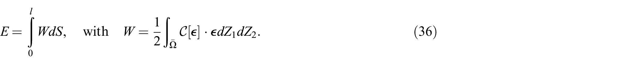
From equations (30)₂, (32), and the Dominated Convergence Theorem, we then have that:

$$\underset{h\to 0}{lim}\left(\frac{\mathcal{E}}{h^4}\right)=E,$$

(35)

where:

$$E=\underset{0}{\overset{l}{\int }}\mathrm{WdS},\mathrm{with}W=\frac{1}{2}{\int }_{\overline{\mathrm{\Omega }}}\mathcal{C}[ϵ]·ϵd{Z}_{1}d{Z}_2.$$

(36)

Accordingly,

$$\mathcal{E}=h^{4}E+o(h^4)$$

(37)

and $h^{4}E$ is the leading-order strain energy for small $h.$

3.2. The optimum energy for a given flexure-twist strain

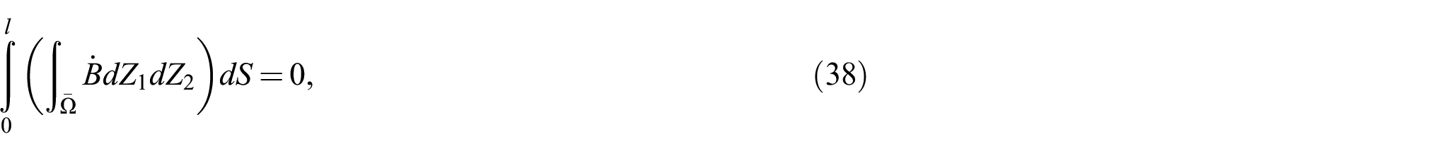
Let $B(\nabla \mathit{\phi })=(1/2)\mathcal{C}[ϵ]·ϵ$ with $\mathit{\gamma }$ fixed. Equation (37) implies that at leading order in $h,$ $\mathit{\phi }$ minimizes the energy $\mathcal{E}$ if and only if it minimizes $E$ , and hence only if it renders $E$ stationary. Accordingly, minimizers satisfy:

$$\underset{0}{\overset{l}{\int }}\left({\int }_{\overline{\mathrm{\Omega }}}\stackrel{·}{B}d{Z}_{1}d{Z}_2\right)\mathrm{dS}=0,$$

(38)

where:

$$\stackrel{·}{B}=\mathit{S}·\stackrel{·}{ϵ},\mathrm{with}\mathit{S}=\mathcal{C}[ϵ]\mathrm{and}\stackrel{·}{ϵ}=\nabla \stackrel{·}{\mathit{\phi }}={\stackrel{·}{\mathit{\phi }}}_{,\alpha }\otimes {\mathit{E}}_{\alpha },$$

(39)

where a superposed dot is used to denote a variational derivative. Here, to ensure compliance with equation (7), we fix $\mathit{R}$ (see equation (34)) and minimize in the class of functions $\mathit{\phi }$ that vanish, together with their derivatives, at the curve of centroids. An explicit example of such a function is given in section 3.3. The structure of $\nabla \stackrel{·}{\mathit{\phi }}$ implies that:

$$\stackrel{·}{B}=\mathit{S}1·\nabla \stackrel{·}{\mathit{\phi }},\mathrm{where}1=\mathit{I}-{\mathit{E}}_3\otimes {\mathit{E}}_3,$$

(40)

is the projection onto the plane $\overline{\mathrm{\Omega }}$ , and an application of Green’s theorem yields that equation (38) is equivalent, granted sufficient regularity, to the local conditions:

$$\mathrm{div}(\mathit{S}1)=0\mathrm{in}\overline{\mathrm{\Omega }}\mathrm{and}\mathit{S}1\mathit{\nu }=0\mathrm{on}\partial \overline{\mathrm{\Omega }},$$

(41)

where $\mathrm{div}$ is the two-dimensional divergence with respect to $\mathit{Z}$ , and $\mathit{\nu }$ is the exterior unit normal to $\partial \overline{\mathrm{\Omega }}$ .

To show that solutions $\mathit{\phi }(Z_{\alpha },S)$ to equation (41) are minimizers, we introduce a one-parameter family $\mathit{\phi }(Z_{\alpha },S;t)$ , with $t\in [0,1]$ , and define $\sigma (t)=B(\nabla \mathit{\phi }(Z_{\alpha },S;t))$ at fixed $Z_{\alpha },S$ . Consider the particular family defined by:

$$\mathit{\phi }(Z_{\alpha },S;t)=(1-t)\mathit{\phi }(Z_{\alpha },S)+t\mathit{\psi }(Z_{\alpha },S).$$

(42)

The derivatives of $\sigma$ are $\stackrel{·}{\sigma }=\mathcal{C}[ϵ(t)]·\nabla \stackrel{·}{\mathit{\phi }}$ and $\stackrel{··}{\sigma }=\mathcal{C}[\nabla \stackrel{·}{\mathit{\phi }}]·\nabla \stackrel{·}{\mathit{\phi }}$ , where $\stackrel{·}{\mathit{\phi }}=\mathit{\psi }-\mathit{\phi }$ and $\mathbf{ϵ}(\mathbf{t})$ is given by equation (33) in which $\mathit{\phi }$ replaced by $\mathit{\phi }(Z_{\alpha },S;t)$ . It follows that $\stackrel{··}{\sigma }\ge 0$ , and hence that:

$$\stackrel{·}{\sigma }(t)=\stackrel{·}{\sigma }(0)+\underset{0}{\overset{t}{\int }}\stackrel{··}{\sigma }\mathrm{dx}\ge \stackrel{·}{\sigma }(0)\mathrm{and}\sigma (1)=\sigma (0)+\underset{0}{\overset{1}{\int }}\stackrel{·}{\sigma }(t)\mathrm{dt}\ge \sigma (0)+\stackrel{·}{\sigma }(0),$$

(43)

the second inequality being equivalent to:

$$B(\nabla \mathit{\psi })-B(\nabla \mathit{\phi })\ge \mathit{S}1·\nabla (\mathit{\psi }-\mathit{\phi }).$$

(44)

Integrating this over $\overline{\mathrm{\Omega }}$ and then over $[0,l]$ we conclude, with equations (38) and (40), that solutions to equation (41) furnish global minimizers of the energy at fixed $\mathit{\gamma }$ .

3.3. Isotropy

Before specializing equation (41) to isotropic materials, we first reduce them using the representation:

$$\mathit{S}=\mathit{SI}=\mathit{S}1+\mathit{S}{\mathit{E}}_3\otimes {\mathit{E}}_3,$$

(45)

invoking the symmetry of $\mathit{S}$ , and equating this expression to its transpose. Multiplying the resulting equality on the right by $1$ , on noting that $1^2=1$ , we obtain:

$$\mathit{S}1=\mathit{\sigma }+{\mathit{E}}_3\otimes 1\mathit{S}{\mathit{E}}_3,\mathrm{where}\mathit{\sigma }=1\mathit{S}1.$$

(46)

Then, because ${\mathit{E}}_3$ does not depend on $\mathit{Z}$ , equation (41) is seen to be equivalent to the system:

$$\begin{array}{c}\mathrm{div}\mathit{\sigma }=0\mathrm{and}\mathrm{div}(1\mathit{S}{\mathit{E}}_3)=0\mathrm{in}\overline{\mathrm{\Omega }};\hfill \\ \mathit{\sigma }\mathit{\nu }=0\mathrm{and}1\mathit{S}{\mathit{E}}_3·\mathit{\nu }=0\mathrm{on}\partial \overline{\mathrm{\Omega }}.\hfill \end{array}$$

(47)

In the case of isotropy, it follows from equations (31), (33), and (39)₂ that:

$$\mathit{S}=\lambda ({\mathit{E}}_3·\mathit{\gamma }\times \mathit{Z}+\mathrm{div}\mathit{\phi })\mathit{I}+\mu [\mathit{\gamma }\times \mathit{Z}\otimes {\mathit{E}}_3+{\mathit{E}}_3\otimes \mathit{\gamma }\times \mathit{Z}+\nabla \mathit{\phi }+{(\nabla \mathit{\phi })}^t],$$

(48)

and hence that:

$$\mathit{\sigma }=\lambda ({\mathit{E}}_3·\mathit{\gamma }\times \mathit{Z}+\mathrm{div}\mathit{\phi })1+\mu [1\nabla \mathit{\phi }+{(\nabla \mathit{\phi })}^{t}1]\mathrm{and}1\mathit{S}{\mathit{E}}_3=\mu [1(\mathit{\gamma }\times \mathit{Z})+{(\nabla \mathit{\phi })}^t{\mathit{E}}_3].$$

(49)

With:

$$\mathit{\gamma }={\gamma }_i{\mathit{E}}_i\mathrm{and}\mathit{\phi }={\phi }_i{\mathit{E}}_i,$$

(50)

it is then straightforward to verify that:

$$\mathit{\sigma }=[\lambda (e_{\gamma \mu }{\gamma }_{\gamma }{Z}_{\mu }+{\phi }_{\mu ,\mu }){\delta }_{\alpha \beta }+\mu ({\phi }_{\alpha ,\beta }+{\phi }_{\beta ,\alpha })]{\mathit{E}}_{\alpha }\otimes {\mathit{E}}_{\beta }\mathrm{and}1\mathit{S}{\mathit{E}}_3=\mu ({\gamma }_3{e}_{\alpha \beta }{Z}_{\alpha }+{\phi }_{3,\beta }){\mathit{E}}_{\beta },$$

(51)

where ${\delta }_{\alpha \beta }$ and $e_{\alpha \beta }$ , respectively, are the two-dimensional Kronecker delta and permutation symbols.

As is well known [12], the functions:

$${\phi }_1=-\nu {\gamma }_1{Z}_1{Z}_2+\frac{1}{2}\nu {\gamma }_2(Z_1^2-Z_2^2),{\phi }_2=\nu {\gamma }_2{Z}_1{Z}_2+\frac{1}{2}\nu {\gamma }_1(Z_1^2-Z_2^2),$$

(52)

where:

$$\nu =\frac{\lambda }{2(\lambda +\mu )},$$

(53)

is Poisson’s ratio, furnish $\mathit{\sigma }=0$ and thus yield a solution to equations (47)₁ and (47)₃, whereas equations (47)₂ and (47)₄ reduce, respectively, to:

$$\mathrm{\Delta }w=0\mathrm{in}\overline{\mathrm{\Omega }}\mathrm{and}(w_{,1}-Z_2){\nu }_1+(w_{,2}+Z_1){\nu }_2=0\mathrm{on}\partial \overline{\mathrm{\Omega }},$$

(54)

where $\mathrm{\Delta }(·)={(·)}_{,\alpha \alpha }$ is the two-dimensional Laplacian with respect to $\mathit{Z}$ and $w(Z_{\alpha })$ , defined by:

$${\phi }_3(Z_{\alpha },S)={\gamma }_3(S)w(Z_{\alpha }),$$

(55)

is the classical St. Venant warping function for torsion of a prismatic cylinder.

Let $w$ be a solution to equation (54) and let $w_0=w(Z_1-C_1,Z_2-C_2)$ , where $C_{\alpha }$ are the constants. Then, as is well known, $w$ and $w_0+Z_1{C}_2-Z_2{C}_1$ satisfy the same Neumann problem [19], and therefore differ by a constant, $C$ say. The constants $C$ and $C_{\alpha }$ may be adjusted to give $w_{|c}=0$ and $\nabla w_{|c}=0$ to ensure, together with equations (34)₁ and (52), that the requirements (7)_1,2 are satisfied.

To derive an expression for the energy $W$ in equation (36), we use equations (31) and (33) to write: ²

$$\frac{1}{2}\mathcal{C}[ϵ]·ϵ=\frac{1}{2}E({\gamma }_2{Z}_1-{\gamma }_1{Z}_2{)}^2+\frac{1}{2}\mu [{(w_{,1}-Z_2)}^2+{(w_{,2}+Z_1)}^2]{\gamma }_3^2,$$

(56)

where:

$$E=\frac{\mu (3\lambda +2\mu )}{\lambda +\mu }$$

(57)

is Young’s modulus. Then, choosing the ${\mathit{E}}_{\alpha }$ to be aligned with the principal axes of $\mathrm{\Omega }$ , i.e.,

$${\int }_{\overline{\mathrm{\Omega }}}{Z}_1{Z}_{2}d{Z}_{1}d{Z}_2=0,$$

(58)

we obtain:

$$W=\frac{1}{2}E({\overline{I}}_1{\gamma }_1^2+{\overline{I}}_2{\gamma }_2^2)+\frac{1}{2}\mu \overline{J}{\gamma }_3^2,$$

(59)

where: ³

$${\overline{I}}_1={\int }_{\overline{\mathrm{\Omega }}}{Z}_2^{2}d{Z}_{1}d{Z}_2,{\overline{I}}_2={\int }_{\overline{\mathrm{\Omega }}}{Z}_1^{2}d{Z}_{1}d{Z}_2\mathrm{and}\overline{J}={\int }_{\overline{\mathrm{\Omega }}}(Z_1^2+Z_2^2+Z_1{w}_{,2}-Z_2{w}_{,1})d{Z}_{1}d{Z}_2.$$

(60)

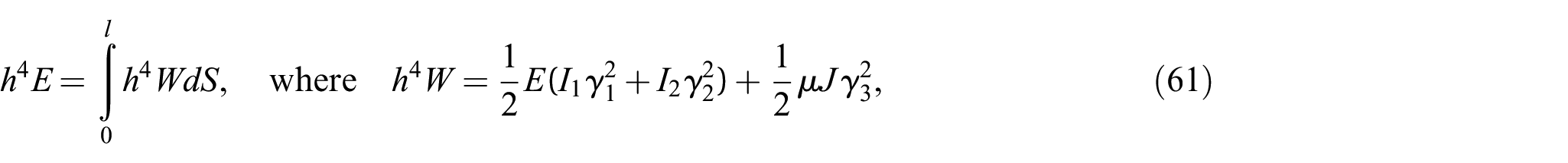
Finally, the leading-order strain energy is given by:

$$h^{4}E=\underset{0}{\overset{l}{\int }}{h}^4\mathrm{WdS},\mathrm{where}{h}^{4}W=\frac{1}{2}E(I_1{\gamma }_1^2+I_2{\gamma }_2^2)+\frac{1}{2}\mu J{\gamma }_3^2,$$

(61)

with $I_{1,2}=h^4{\overline{I}}_{1,2}$ and $J=h^4\overline{J}.$

With equation (61) in hand, the use of the virtual power principle to extract the equations of equilibrium or motion, together with the forms of the relevant forces and moments acting on the rod, is a well-known exercise (see Antman [2], O’Reilly [3] and Steigmann and Faulkner [20], for example).

4. Plastic deformation of initially straight, untwisted rods

To model the elastic response of a uniform material that has been plastically deformed, we write the strain energy $\mathrm{\Psi }$ , per unit volume of the reference configuration $\kappa$ , in the form [21,22]:

$$\mathrm{\Psi }=(det\mathit{K}{)}^{-1}U(\mathit{H}),\mathrm{where}\mathit{H}=\mathit{FK}$$

(62)

is the elastic part of the deformation and ${\mathit{K}}^{-1}$ is the plastic part. As is well known, in general, neither the elastic nor the plastic part is a gradient. The Cauchy stress $\mathit{T}$ is given by $U_{\mathit{H}}=\mathit{T}{\mathit{H}}^{*}$ , and we impose the same restrictions on the function $U(\mathit{H})$ that we imposed on $\mathrm{\Psi }(\mathit{F})$ in section 3.1, i.e., $U(\mathit{H})=U(\mathit{QH})$ for all rotations $\mathit{Q}$ , together with $U(\mathit{I})=0$ and $U_{\mathit{H}}(\mathit{I})=0$ . We then have [22] $U_{\mathit{HH}}(\mathit{I})[\mathit{A}]=\mathcal{C}[\mathit{A}]$ for any tensor $\mathit{A}$ , where $\mathcal{C}$ is again the classical fourth-order tensor of elastic moduli, given, in the case of isotropy, by equation (31).

In place of equation (18), we now assume that the restriction to the centroidal axis of the elastic deformation is a pure rotation, i.e.,

$${\mathit{H}}_{|c}=\mathit{R}(S)\in \mathrm{Ort}{h}^{+}.$$

(63)

This implies, with $U_{\mathit{H}}(\mathit{R})=\mathit{R}{U}_{\mathit{H}}(\mathit{I})$ , that ${\mathit{T}}_{|c}$ vanishes. Typical plastic flow rules [22] then yield that the material time derivative ${\stackrel{.}{\underset{~}{\mathit{K}}}}_{|c}$ vanishes, and hence that ${\mathit{K}}_{|c}$ retains its initial value. Taking this value to be $\mathit{I}$ , we conclude that equations (18)–(22) remain in effect with $\mathit{\gamma }$ replaced by $\mathbf{\kappa }$ if the rod is naturally straight and untwisted, i.e., if $\overline{\kappa }=0$ . In accordance with these conditions, we assume that:

$$\mathit{K}=\mathit{I}+h\mathit{L}(Z_{\alpha },S;h)\mathrm{with}{\mathit{L}}_{|c}=0.$$

(64)

For example, if $\mathit{K}$ is differentiable with respect to the $X_{\alpha }$ , then:

$$\mathit{L}=Z_{\alpha }{\mathit{K}}_{\alpha }(S)+h^{-1}\mathit{o}(h),\mathrm{where}{\mathit{K}}_{\alpha }=\frac{\partial }{\partial X_{\alpha }}{\mathit{K}}_{|c}.$$

(65)

We then find that (see equations (26) and (27)):

$$\mathit{H}=\mathit{R}(\mathit{I}+\mathit{E}),\mathrm{with}\mathit{E}=h[\mathbf{\kappa }\times \mathit{Z}\otimes {\mathit{E}}_3+\nabla ({\mathit{R}}^t\mathit{u})+\mathit{L}]+\mathit{o}(h);$$

(66)

and, with $(det\mathit{K}{)}^{-1}=1-\mathrm{htr}\mathit{L}+o(h)$ , that equations (36) and (37) remain in effect with:

$$\mathbf{ϵ}=\mathbf{\kappa }\times \mathit{Z}\otimes {\mathit{E}}_3+\nabla \mathit{\phi }+Z_{\alpha }{\mathit{K}}_{\alpha },$$

(67)

and with $\mathit{\phi }$ as in equation (34).

Proceeding exactly as in section 3.1, again we conclude that the energy is optimized by functions $\mathit{\phi }$ satisfying equation (41), but with $\mathit{S}$ now given by:

$$\mathit{S}=\mathcal{C}[\mathbf{\kappa }\times \mathit{Z}\otimes {\mathit{E}}_3+\nabla \mathit{\phi }+Z_{\alpha }{\mathit{K}}_{\alpha }].$$

(68)

Solutions, substituted into equations (36) and (67), deliver the optimal energy density $W$ in terms of $\mathbf{\kappa }$ and ${\mathit{K}}_{\alpha }$ .

It is shown in Kaczmarski et al. [15], for isotropic materials and in the context of growth mechanics, that the function $W$ thus derived may be recast in the form (61), with appropriate values of the components of $\overline{\kappa }$ . Here, we are content to exhibit restrictions on the ${\mathit{K}}_{\alpha }$ which are such as to furnish sufficient conditions for such correspondence. Thus, fixing $\mathit{\phi }$ and $\mathbf{\kappa }$ and comparing equations (33) and (67), on noting equation (24), it is clear that a sufficient condition for the energy associated with the initially straight, plastically deformed rod to reduce to that of the naturally curved and twisted purely elastic rod is:

$$Z_{\alpha }\mathrm{Sym}{\mathit{K}}_{\alpha }+\mathrm{Sym}(\overline{\kappa }\times \mathit{Z}\otimes {\mathit{E}}_3)=0,$$

(69)

in which the prefix $\mathrm{Sym}$ stems from the minor symmetries of the elasticity tensor $\mathcal{C}.$ On differentiating with respect to the $Z_{\beta }$ , we reach:

$$\begin{array}{c}\mathrm{Sym}{\mathit{K}}_1=\alpha (S)({\mathit{E}}_2\otimes {\mathit{E}}_3+{\mathit{E}}_3\otimes {\mathit{E}}_2)+\beta (S){\mathit{E}}_3\otimes {\mathit{E}}_3,\hfill \\ \mathrm{Sym}{\mathit{K}}_2=-\alpha (S)({\mathit{E}}_1\otimes {\mathit{E}}_3+{\mathit{E}}_3\otimes {\mathit{E}}_1)+\gamma (S){\mathit{E}}_3\otimes {\mathit{E}}_3,\hfill \end{array}$$

(70)

where $\alpha ,\beta ,\gamma$ are the arbitrary functions, and:

$${\overline{\kappa }}_1=-\gamma ,{\overline{\kappa }}_2=\beta \mathrm{and}{\overline{\kappa }}_3=-2\alpha .$$

(71)

The skew parts of the ${\mathit{K}}_{\alpha }$ are not restricted.