A benchmark strain gradient elasticity solution in two-dimensions for verifying computational approaches by means of the finite element method

Abstract

In elasticity, microstructure-related deviations may be modeled by strain gradient elasticity. For so-called metamaterials, different implementations are possible for solving strain gradient elasticity problems numerically. Analytical solutions of simple problems are used to verify the numerical approach. We demonstrate such a case in a two-dimensional continuum as a benchmark case for computations. As strain gradient enforces higher regularity conditions in displacements, in the finite element method (FEM), the use of standard elements is often seen as inadequate. For such piecewise or elementwise continuous elements, we examine a possible remedy to correctly simulate strain gradient elasticity problems by implementing two techniques. First, we enforce continuity of displacement gradient across elements; second, we employ a mixed finite element method where displacement and its gradient are solved both as unknowns. The results show the pros and cons of each numerical technique. All methods converge monotonically, but the mixed method is more reliable than the other one.

1. Introduction

Accurate modeling of materials at microscopic length scale is necessary for design and engineering of structures with a detailed and complex substructure. The first-order (first-gradient) continuum mechanics depends on displacement and its first gradient; however, it lacks accuracy at the scales which are close to the length scale of the substructure [1], especially in capturing those phenomena which are dependent on geometric length, known as size effect. A generalization of the first-order elasticity theory is an approach for overcoming this issue. In generalized continuum mechanics, the governing equation depends on displacement, first gradient of displacement, and second gradient of displacement.

The idea of generalized mechanics dates back to the beginning of 20th century, see [2,3] for a history. Modern theories were introduced later starting around six decades ago [4–7]. Since then, many generalized mechanics theories have been proposed, and they can be considered as specific cases of a unified theory [8].

Generalized mechanics has been widely investigated in the literature. It has been implemented for problems of elasticity [9–13]; plasticity [14–19]; damage modeling [20–25]; modeling metamaterials [26–28] such as pantographic structures [29–31], network materials [32], viscoelastic truss structures [33], bi-pantographic structures [34], second gradient fluids [35]; gradient-enhanced homogenization [36–39]; micropolar continua [40]; fracture mechanics [41]; biomechanics [42–44]; and anisotropic systems [45]. Parameter determination of generalized mechanics models has been studied for static and dynamic regimes in Shekarchizadeh et al. [46, 47], respectively.

Including higher gradients of displacement in the equations results in partial differential equations of higher order. A reliable numerical computation of such equations requires suitable techniques and element type selection that ensure the monotonous convergence. For this purpose, different numerical approaches have been proposed for the strain gradient theories such as isogeometric analysis [47–50], $C^1$ continuous elements [52,53], and mixed finite element formulation [54–56]. It is beneficial to verify the computations by analytical solutions. The analytical solutions for some example problems in the generalized continua are presented, for example, in previous studies [57–61].

In this paper, a two-dimensional problem in the framework of the strain gradient elasticity theory is solved numerically, by means of a finite element method (FEM) implemented using open-source FEniCS libraries. Different techniques are used for the implementation of the numerical code including using mixed finite element formulation, using Lagrange multipliers for imposing the boundary conditions, and enforcing continuity of first gradient across elements. The computations are compared with analytical solutions. Different implementations are compared to each other regarding convergence, computation time, and robustness.

This paper is structured in the following way. First, in Section 2, the strain gradient theory is explained, the weak form is generated to be used in the analytical solution, and the constitutive equations are presented. Then, in Section 3, an analytical solution is presented for a plate under simple shear with two different sets of boundary conditions. Next, in Section 4, the numerical implementation and weak form generation of FEM and Mixed FEM are sketched in detail. Finally, the results and error analyses of two implementations of the strain gradient elasticity theory are shown in Section 5.

2. Strain gradient elasticity

2.1. Weak form generation

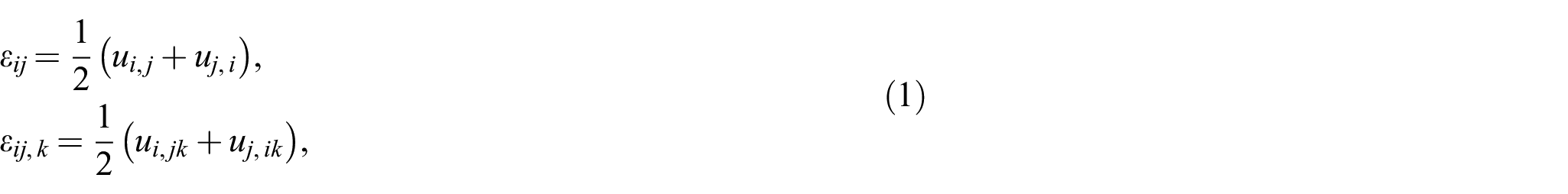
One of the well-known generalizations of the conventional continuum mechanics is the strain gradient elasticity theory. In this theory, the energy density depends not only on strain, ${\epsilon }_{\mathrm{ij}}$ , but also on its gradient, ${\epsilon }_{\mathrm{ij},k}$ , where

$$\begin{array}{cc}\multicolumn{1}{c}{}& {\epsilon }_{\mathrm{ij}}=\frac{1}{2}(u_{i,j}+u_{j,i}),\hfill \\ \multicolumn{1}{c}{}& {\epsilon }_{\mathrm{ij},k}=\frac{1}{2}(u_{i,\mathrm{jk}}+u_{j,\mathrm{ik}}),\hfill \end{array}$$

(1)

where $u_i$ is the displacement field and the comma indicates differentiation in space, $\mathit{X}\in \mathrm{\Omega }\subset {\mathrm{I}\mathrm{R}}^3$ , in Cartesian coordinates. Therefore, we have

$$\begin{array}{cc}\multicolumn{1}{c}{}& u_{i,j}=\frac{\partial u_i}{\partial X_j},\hfill \\ \multicolumn{1}{c}{}& u_{i,\mathrm{jk}}={\left(u_{i,j}\right)}_{,k}=\frac{\partial }{\partial X_k}\left(\frac{\partial u_i}{\partial X_j}\right)=\frac{{\partial }^2{u}_i}{\partial X_k\partial X_j}.\hfill \end{array}$$

(2)

In equation (1), the geometric nonlinearities are neglected since the strain measure has to be linear for deriving an analytical solution in the following. We begin with the general formulation based on a scalar mathematical construct called action $\mathcal{A}$ . We postulate the action in the time interval $\mathcal{T}$ as

$$\mathcal{A}={\int }_{\mathcal{T}}({\int }_{\mathrm{\Omega }}\mathcal{L}\mathrm{d}V+{\int }_{\partial \mathrm{\Omega }}{W}_s\mathrm{d}A+{\int }_{\partial \partial \mathrm{\Omega }}{W}_e\mathrm{d}L)\mathrm{d}t,$$

(3)

over the domain, $\mathrm{\Omega }$ , with its boundary, $\partial \mathrm{\Omega }$ , and the set $\partial \partial \mathrm{\Omega }$ of the edges of the boundary surface. In a three-dimensional problem, the terms $W_s$ and $W_e$ are the work done on the boundary surface elements, $\mathrm{d}A$ , and line (edge) elements, $\mathrm{d}L$ , respectively. Herein, we neglect the term $W_e$ for simplicity [62,63]. The values of $W_s$ are known, and as this term is applied on the boundary, for the same accuracy in an expansion up to the second order in space derivative, we set $W_s=W_s(u_i,u_{i,j})$ , i.e., depending only on the displacement and its first gradient but not on the second gradient.

In equation (3), $\mathcal{L}$ is an existing Lagrangean density describing the underlying system. In the strain gradient elasticity theory for an elastic material, as discussed in Abali [64], we consider the Lagrangean density as

$$\mathcal{L}=\frac{1}{2}{\rho }_0({\stackrel{·}{u}}_i{\stackrel{·}{u}}_i+d^2{\stackrel{·}{u}}_{i,j}{\stackrel{·}{u}}_{i,j}+{\tau }^2{\stackrel{··}{u}}_i{\stackrel{··}{u}}_i)-w+{\rho }_0{f}_i{u}_i,$$

(4)

where the first three terms indicate the kinetic energy (inertial terms). The term $w$ is the stored (deformation) energy density in $\mathrm{J}/{\mathrm{m}}^3$ . For homogeneous materials, the stored energy density reads

$$w=w(u_{i,j},u_{i,\mathrm{jk}}).$$

(5)

The last term in equation (4) denotes the potential energy with the specific body force, $f$ , in N/kg. Based on the principle of least action, for reversible systems, we are looking for solutions such that the variation of the action functional vanishes for any arbitrary test function $\delta \mathit{u}$

$$\delta \mathcal{A}=0\forall \delta \mathit{u}.$$

(6)

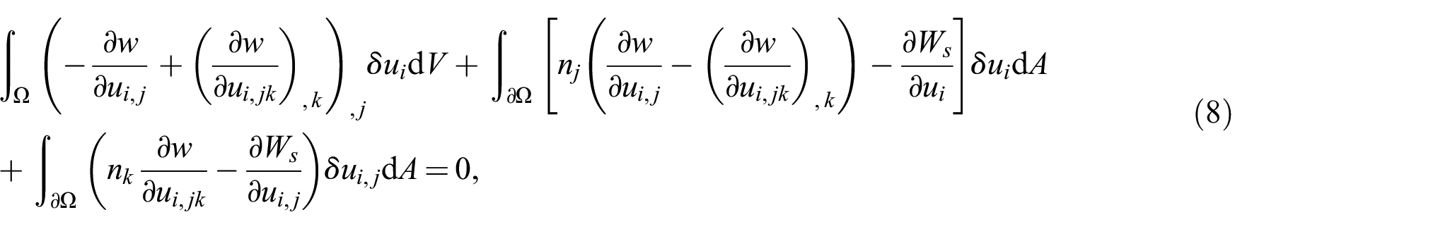
The variation of the action, $\delta \mathcal{A}$ , is derived by employing Taylor’s expansion with respect to a suitable perturbation parameter, as explained in Abali et al. [65]. By inserting $\mathcal{A}$ from equation (3) in equation (6), and neglecting the inertial terms, body forces, and boundary terms acting on edges, according to the least action principle, the integral form for the second-order strain gradient elasticity for a domain $\mathrm{\Omega }$ reads

$$-{\int }_{\mathrm{\Omega }}(\frac{\partial w}{\partial u_{i,j}}\delta u_{i,j}+\frac{\partial w}{\partial u_{i,\mathrm{jk}}}\delta u_{i,\mathrm{jk}})\mathrm{d}V+{\int }_{\partial \mathrm{\Omega }}(\frac{\partial W_s}{\partial u_i}\delta u_i+\frac{\partial W_s}{\partial u_{i,j}}\delta u_{i,j})\mathrm{d}A=0.$$

(7)

After applying the product rule and the divergence (Gauss’s) theorem multiple times (for details see Appendix 1), we obtain

$$\begin{array}{cc}\multicolumn{1}{c}{}& {\int }_{\mathrm{\Omega }}{(-\frac{\partial w}{\partial u_{i,j}}+{\left(\frac{\partial w}{\partial u_{i,\mathrm{jk}}}\right)}_{,k})}_{,j}\delta u_i\mathrm{d}V+{\int }_{\partial \mathrm{\Omega }}[n_j(\frac{\partial w}{\partial u_{i,j}}-{\left(\frac{\partial w}{\partial u_{i,\mathrm{jk}}}\right)}_{,k})-\frac{\partial W_s}{\partial u_i}]\delta u_i\mathrm{d}A\hfill \\ \multicolumn{1}{c}{}& +{\int }_{\partial \mathrm{\Omega }}(n_k\frac{\partial w}{\partial u_{i,\mathrm{jk}}}-\frac{\partial W_s}{\partial u_{i,j}})\delta u_{i,j}\mathrm{d}A=0,\hfill \end{array}$$

(8)

since, as already remarked, the inertial terms, body forces, and boundary terms acting on edges are neglected. Here, $n$ is the outward unit normal to the boundary $\partial \mathrm{\Omega }$ . We define $W_s$ on Neumann boundaries as

$$W_s=t_i{u}_i+m_{\mathrm{ij}}{u}_{i,j},$$

(9)

where $t$ , in N/m² (traction), and $m$ , in N m/m² (double traction), satisfy the following conditions

$$t_i=\frac{\partial W_s}{\partial u_i}=n_j(\frac{\partial w}{\partial u_{i,j}}-{\left(\frac{\partial w}{\partial u_{i,\mathrm{jk}}}\right)}_{,k}),$$

(10)

$$m_{\mathrm{ij}}=\frac{\partial W_s}{\partial u_{i,j}}=n_k\frac{\partial w}{\partial u_{i,\mathrm{jk}}}.$$

(11)

By inserting equations (10) and (11) in equation (8), the following governing equation is obtained

$${(\frac{\partial w}{\partial u_{i,j}}-{\left(\frac{\partial w}{\partial u_{i,\mathrm{jk}}}\right)}_{,k})}_{,j}=0,$$

(12)

which is solved numerically to calculate the displacement field in the domain $\mathrm{\Omega }$ .

2.2. Constitutive laws

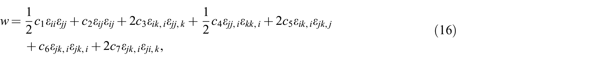
The stored energy density, $w$ , in equation (12), for centro-symmetric materials is expressed as

$$w=w({\epsilon }_{\mathrm{ij}},{\epsilon }_{\mathrm{ij},k})=\frac{1}{2}{\epsilon }_{\mathrm{ij}}{C}_{\mathrm{ijkl}}{\epsilon }_{\mathrm{kl}}+\frac{1}{2}{\epsilon }_{\mathrm{ij},k}{D}_{\mathrm{ijklmn}}{\epsilon }_{\mathrm{lm},n},$$

(13)

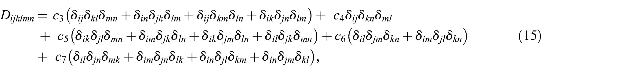
where $C_{\mathrm{ijkl}}$ denotes the rank-4 stiffness tensor (first gradient), and $D_{\mathrm{ijklmn}}$ indicates the rank-6 strain gradient stiffness tensor (second gradient) [66–70]. For isotropic materials, we have

$$C_{\mathrm{ijkl}}=c_1{\delta }_{\mathrm{ij}}{\delta }_{\mathrm{kl}}+c_2({\delta }_{\mathrm{ik}}{\delta }_{\mathrm{jl}}+{\delta }_{\mathrm{il}}{\delta }_{\mathrm{jk}}),$$

(14)

$$\begin{array}{cc}\multicolumn{1}{c}{D_{\mathrm{ijklmn}}}& =c_3({\delta }_{\mathrm{ij}}{\delta }_{\mathrm{kl}}{\delta }_{\mathrm{mn}}+{\delta }_{\mathrm{in}}{\delta }_{\mathrm{jk}}{\delta }_{\mathrm{lm}}+{\delta }_{\mathrm{ij}}{\delta }_{\mathrm{km}}{\delta }_{\ln }+{\delta }_{\mathrm{ik}}{\delta }_{\mathrm{jn}}{\delta }_{\mathrm{lm}})+c_4{\delta }_{\mathrm{ij}}{\delta }_{\mathrm{kn}}{\delta }_{\mathrm{ml}}\hfill \\ \multicolumn{1}{c}{}& +c_5({\delta }_{\mathrm{ik}}{\delta }_{\mathrm{jl}}{\delta }_{\mathrm{mn}}+{\delta }_{\mathrm{im}}{\delta }_{\mathrm{jk}}{\delta }_{\ln }+{\delta }_{\mathrm{ik}}{\delta }_{\mathrm{jm}}{\delta }_{\ln }+{\delta }_{\mathrm{il}}{\delta }_{\mathrm{jk}}{\delta }_{\mathrm{mn}})+c_6({\delta }_{\mathrm{il}}{\delta }_{\mathrm{jm}}{\delta }_{\mathrm{kn}}+{\delta }_{\mathrm{im}}{\delta }_{\mathrm{jl}}{\delta }_{\mathrm{kn}})\hfill \\ \multicolumn{1}{c}{}& +c_7({\delta }_{\mathrm{il}}{\delta }_{\mathrm{jn}}{\delta }_{\mathrm{mk}}+{\delta }_{\mathrm{im}}{\delta }_{\mathrm{jn}}{\delta }_{\mathrm{lk}}+{\delta }_{\mathrm{in}}{\delta }_{\mathrm{jl}}{\delta }_{\mathrm{km}}+{\delta }_{\mathrm{in}}{\delta }_{\mathrm{jm}}{\delta }_{\mathrm{kl}}),\hfill \end{array}$$

(15)

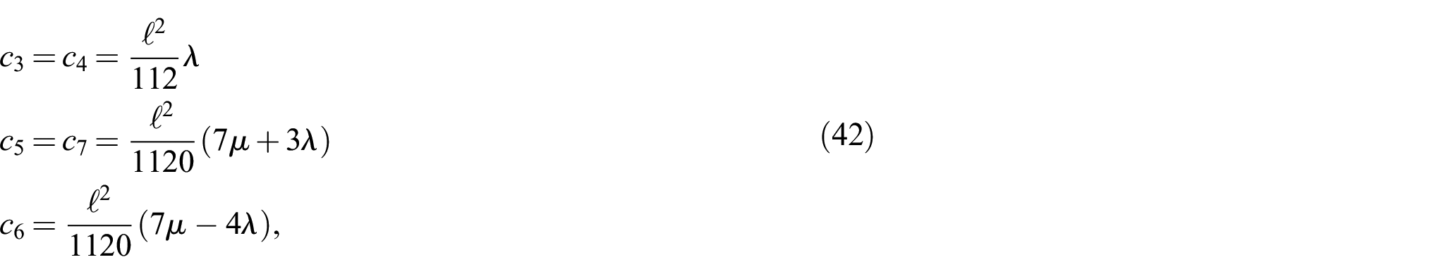
where $c_1,c_2$ are the two Lame constants, and $c_3,c_4,c_5,c_6,c_7$ are five additional parameters characterizing the substructure of the material; we refer to Abali et al. [71] for a derivation of this form. After inserting equations (14) and (15) in equation (13), the stored energy becomes

$$\begin{array}{cc}\multicolumn{1}{c}{}& w=\frac{1}{2}{c}_1{\epsilon }_{\mathrm{ii}}{\epsilon }_{\mathrm{jj}}+c_2{\epsilon }_{\mathrm{ij}}{\epsilon }_{\mathrm{ij}}+2c_3{\epsilon }_{\mathrm{ik},i}{\epsilon }_{\mathrm{jj},k}+\frac{1}{2}{c}_4{\epsilon }_{\mathrm{jj},i}{\epsilon }_{\mathrm{kk},i}+2c_5{\epsilon }_{\mathrm{ik},i}{\epsilon }_{\mathrm{jk},j}\hfill \\ \multicolumn{1}{c}{}& +c_6{\epsilon }_{\mathrm{jk},i}{\epsilon }_{\mathrm{jk},i}+2c_7{\epsilon }_{\mathrm{jk},i}{\epsilon }_{\mathrm{ji},k},\hfill \end{array}$$

(16)

which is equivalent to the potential energy density expressed in Mindlin’s work [72, equation (11.3) on page 71]. There is a one-to-one relation between the material parameters used in our formulation $(c_1,c_2,c_3,c_4,c_5,c_6,c_7)$ and in Mindlin’s formulation $(\tilde{\lambda },\tilde{\mu },{\hat{a}}_1,{\hat{a}}_2,{\hat{a}}_3,{\hat{a}}_4,{\hat{a}}_5)$ as follows:

$$c_1=\tilde{\lambda },c_2=\tilde{\mu },c_3=\frac{1}{2}{\hat{a}}_1,c_4=2{\hat{a}}_2,c_5=\frac{1}{2}{\hat{a}}_3,c_6={\hat{a}}_4,c_7=\frac{1}{2}{\hat{a}}_5.$$

(17)

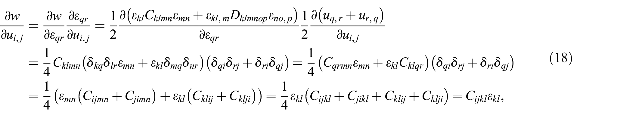
The derivative of the stored energy density with respect to the first gradient of displacement is derived using equations (13), (1), and the chain rule as

$$\begin{array}{cc}\multicolumn{1}{c}{\frac{\partial w}{\partial u_{i,j}}=}& \frac{\partial w}{\partial {\epsilon }_{\mathrm{qr}}}\frac{\partial {\epsilon }_{\mathrm{qr}}}{\partial u_{i,j}}=\frac{1}{2}\frac{\partial ({\epsilon }_{\mathrm{kl}}{C}_{\mathrm{klmn}}{\epsilon }_{\mathrm{mn}}+{\epsilon }_{\mathrm{kl},m}{D}_{\mathrm{klmnop}}{\epsilon }_{\mathrm{no},p})}{\partial {\epsilon }_{\mathrm{qr}}}\frac{1}{2}\frac{\partial (u_{q,r}+u_{r,q})}{\partial u_{i,j}}\hfill \\ \multicolumn{1}{c}{=}& \frac{1}{4}{C}_{\mathrm{klmn}}({\delta }_{\mathrm{kq}}{\delta }_{\mathrm{lr}}{\epsilon }_{\mathrm{mn}}+{\epsilon }_{\mathrm{kl}}{\delta }_{\mathrm{mq}}{\delta }_{\mathrm{nr}})({\delta }_{\mathrm{qi}}{\delta }_{\mathrm{rj}}+{\delta }_{\mathrm{ri}}{\delta }_{\mathrm{qj}})=\frac{1}{4}(C_{\mathrm{qrmn}}{\epsilon }_{\mathrm{mn}}+{\epsilon }_{\mathrm{kl}}{C}_{\mathrm{klqr}})({\delta }_{\mathrm{qi}}{\delta }_{\mathrm{rj}}+{\delta }_{\mathrm{ri}}{\delta }_{\mathrm{qj}})\hfill \\ \multicolumn{1}{c}{=}& \frac{1}{4}({\epsilon }_{\mathrm{mn}}(C_{\mathrm{ijmn}}+C_{\mathrm{jimn}})+{\epsilon }_{\mathrm{kl}}(C_{\mathrm{klij}}+C_{\mathrm{klji}}))=\frac{1}{4}{\epsilon }_{\mathrm{kl}}(C_{\mathrm{ijkl}}+C_{\mathrm{jikl}}+C_{\mathrm{klij}}+C_{\mathrm{klji}})=C_{\mathrm{ijkl}}{\epsilon }_{\mathrm{kl}},\hfill \end{array}$$

(18)

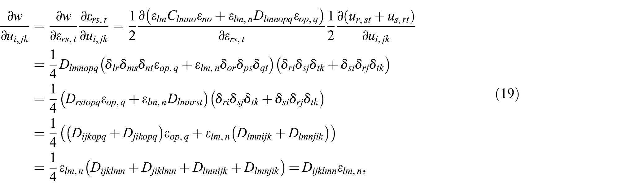
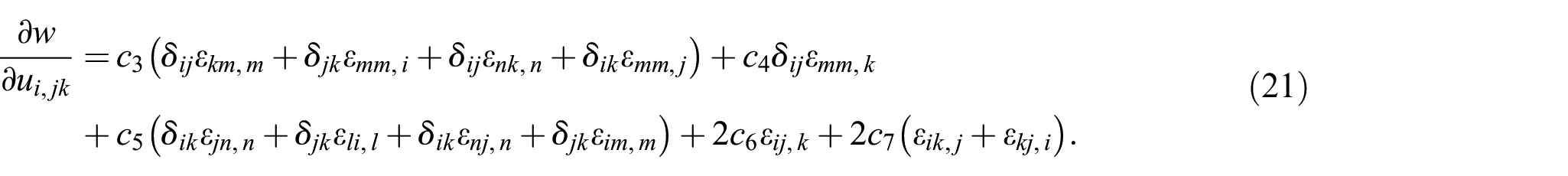
by considering the symmetry of the stiffness tensor $(C_{\mathrm{ijkl}}=C_{\mathrm{jikl}}=C_{\mathrm{klij}}=C_{\mathrm{klji}})$ . In the same way, we get the derivative of the stored energy density with respect to the second gradient of displacement as

$$\begin{array}{cc}\multicolumn{1}{c}{\frac{\partial w}{\partial u_{i,\mathrm{jk}}}=}& \frac{\partial w}{\partial {\epsilon }_{\mathrm{rs},t}}\frac{\partial {\epsilon }_{\mathrm{rs},t}}{\partial u_{i,\mathrm{jk}}}=\frac{1}{2}\frac{\partial ({\epsilon }_{\mathrm{lm}}{C}_{\mathrm{lmno}}{\epsilon }_{\mathrm{no}}+{\epsilon }_{\mathrm{lm},n}{D}_{\mathrm{lmnopq}}{\epsilon }_{\mathrm{op},q})}{\partial {\epsilon }_{\mathrm{rs},t}}\frac{1}{2}\frac{\partial (u_{r,\mathrm{st}}+u_{s,\mathrm{rt}})}{\partial u_{i,\mathrm{jk}}}\hfill \\ \multicolumn{1}{c}{=}& \frac{1}{4}{D}_{\mathrm{lmnopq}}({\delta }_{\mathrm{lr}}{\delta }_{\mathrm{ms}}{\delta }_{\mathrm{nt}}{\epsilon }_{\mathrm{op},q}+{\epsilon }_{\mathrm{lm},n}{\delta }_{\mathrm{or}}{\delta }_{\mathrm{ps}}{\delta }_{\mathrm{qt}})({\delta }_{\mathrm{ri}}{\delta }_{\mathrm{sj}}{\delta }_{\mathrm{tk}}+{\delta }_{\mathrm{si}}{\delta }_{\mathrm{rj}}{\delta }_{\mathrm{tk}})\hfill \\ \multicolumn{1}{c}{=}& \frac{1}{4}(D_{\mathrm{rstopq}}{\epsilon }_{\mathrm{op},q}+{\epsilon }_{\mathrm{lm},n}{D}_{\mathrm{lmnrst}})({\delta }_{\mathrm{ri}}{\delta }_{\mathrm{sj}}{\delta }_{\mathrm{tk}}+{\delta }_{\mathrm{si}}{\delta }_{\mathrm{rj}}{\delta }_{\mathrm{tk}})\hfill \\ \multicolumn{1}{c}{=}& \frac{1}{4}((D_{\mathrm{ijkopq}}+D_{\mathrm{jikopq}}){\epsilon }_{\mathrm{op},q}+{\epsilon }_{\mathrm{lm},n}(D_{\mathrm{lmnijk}}+D_{\mathrm{lmnjik}}))\hfill \\ \multicolumn{1}{c}{=}& \frac{1}{4}{\epsilon }_{\mathrm{lm},n}(D_{\mathrm{ijklmn}}+D_{\mathrm{jiklmn}}+D_{\mathrm{lmnijk}}+D_{\mathrm{lmnjik}})=D_{\mathrm{ijklmn}}{\epsilon }_{\mathrm{lm},n},\hfill \end{array}$$

(19)

by considering the symmetry of the strain gradient stiffness tensor $(D_{\mathrm{lmnijk}}=D_{\mathrm{lmnjik}}=D_{\mathrm{ijklmn}}=D_{\mathrm{jiklmn}})$ . By inserting equation (14) in equation (18), and equation (15) in equation (19), we have

$$\frac{\partial w}{\partial u_{i,j}}=c_1{\delta }_{\mathrm{ij}}{\epsilon }_{\mathrm{kk}}+2c_2{\epsilon }_{\mathrm{ij}},$$

(20)

$$\begin{array}{cc}\multicolumn{1}{c}{\frac{\partial w}{\partial u_{i,\mathrm{jk}}}=}& c_3({\delta }_{\mathrm{ij}}{\epsilon }_{\mathrm{km},m}+{\delta }_{\mathrm{jk}}{\epsilon }_{\mathrm{mm},i}+{\delta }_{\mathrm{ij}}{\epsilon }_{\mathrm{nk},n}+{\delta }_{\mathrm{ik}}{\epsilon }_{\mathrm{mm},j})+c_4{\delta }_{\mathrm{ij}}{\epsilon }_{\mathrm{mm},k}\hfill \\ \multicolumn{1}{c}{+}& c_5({\delta }_{\mathrm{ik}}{\epsilon }_{\mathrm{jn},n}+{\delta }_{\mathrm{jk}}{\epsilon }_{\mathrm{li},l}+{\delta }_{\mathrm{ik}}{\epsilon }_{\mathrm{nj},n}+{\delta }_{\mathrm{jk}}{\epsilon }_{\mathrm{im},m})+2c_6{\epsilon }_{\mathrm{ij},k}+2c_7({\epsilon }_{\mathrm{ik},j}+{\epsilon }_{\mathrm{kj},i}).\hfill \end{array}$$

(21)

Finally, by inserting equations (20) and (21) in equation (12), the governing equation is derived in terms of the material parameters and the gradients of strain as

$$\begin{array}{cc}\multicolumn{1}{c}{}& c_1{\epsilon }_{\mathrm{kk},i}+2c_2{\epsilon }_{\mathrm{ij},j}-c_3(2{\epsilon }_{\mathrm{nk},\mathrm{nki}}+{\epsilon }_{\mathrm{mm},\mathrm{ikk}}+{\epsilon }_{\mathrm{mm},\mathrm{jij}})-c_4{\epsilon }_{\mathrm{mm},\mathrm{kki}}\hfill \\ \multicolumn{1}{c}{}& -2c_5({\epsilon }_{\mathrm{nj},\mathrm{nij}}+{\epsilon }_{\mathrm{im},\mathrm{mkk}})-2c_6{\epsilon }_{\mathrm{ji},\mathrm{kkj}}-2c_7({\epsilon }_{\mathrm{ik},\mathrm{jkj}}+{\epsilon }_{\mathrm{kj},\mathrm{ikj}})=0.\hfill \end{array}$$

(22)

Equation (22) corresponds to the equation of motion derived in Mindlin’s work [72, equation (11.8) on page 72] (with the same one-to-one relation between the material parameters as in equation (17)). Herein, we have neglected the body forces and inertial terms as well.

3. Analytical solution

In this section, the analytical solution for a plate under simple shear is derived. Two cases of loading and boundary conditions are investigated.

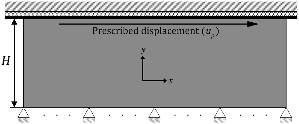
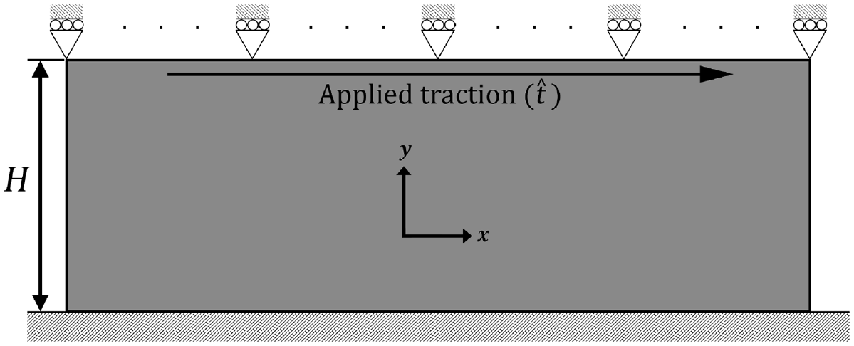
Consider a two-dimensional plate under simple shear as in Figures 1 and 2 with infinite length in $x$ -direction, and with height $H$ in $y$ -direction. The bottom edge is fixed in both directions while the top edge is fixed only in vertical $\left(y\right)$ direction, and a displacement or traction is applied on the top edge in $x$ -direction.

Figure 1.

The plate (infinitely long in $x$ -direction) under simple shear with the boundary conditions stated in equation (26). The top edge is moving in a rail, therefore its rotation is not allowed.

Figure 2.

The plate (infinitely long in $x$ -direction) under simple shear with the boundary conditions stated in equation (33).

Considering the boundary conditions of this problem, only $u_x$ and its derivatives along $y$ -direction are non-zero. This so-called semi-analytical ansatz reduces the problem to a one-dimensional continuum. Therefore, the problem is one-dimensional with $u_y=0$ , $u_x=u_x\left(y\right)=u$ . Hence, we have $u_{x,y}=u\prime$ , $u_{x,\mathrm{yy}}=u″$ , $u_{x,\mathrm{yyy}}=u″\prime$ , $u_{x,\mathrm{yyyy}}=u″″$ , and

$${\epsilon }_{\mathrm{ij}}=\frac{u_{i,j}+u_{j,i}}{2}=\frac{1}{2}\left[\begin{array}{cc}0\hfill & u\prime \hfill \\ \multicolumn{1}{c}{u\prime }& 0\hfill \end{array}\right].$$

(23)

Using equation (22), the governing equation for this problem is formed as

$$c_{2}u″-(c_5+c_6+c_7)u″″=0,$$

(24)

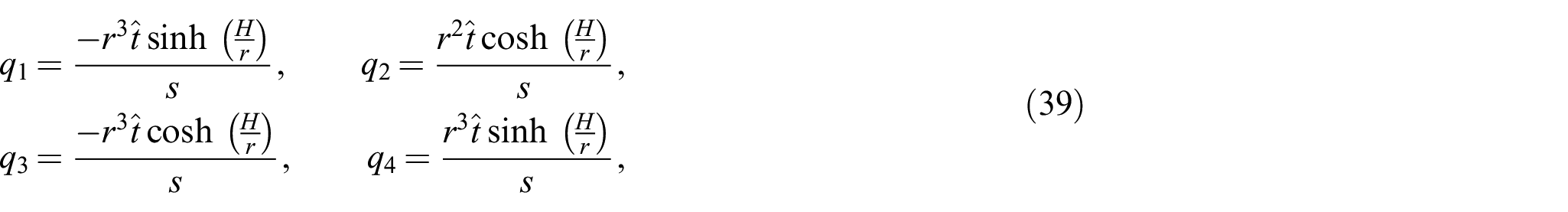
which is a fourth-order ordinary differential equation, and its general solution is

$$u=u_x\left(y\right)=q_1+q_{2}y+q_3\sinh \left(\frac{y}{r}\right)+q_4\cosh \left(\frac{y}{r}\right),$$

(25)

where $r=\sqrt{(c_5+c_6+c_7)/c_2}$ and $q_1,q_2,q_3,q_4$ are four integration constants. Four boundary conditions are necessary for finding $q_1,q_2,q_3,q_4$ . In the following, two sets of boundary conditions are discussed.

3.1. Case 1: displacement prescription

In the first case, as shown in Figure 1, the boundary conditions are considered as

$$u_x\left(0\right)=0,u_x\left(H\right)=\hat{u},m_{\mathrm{xy}}\left(0\right)=0,u\prime \left(H\right)=0,$$

(26)

where a Dirichlet boundary condition is assumed on the top edge by applying a displacement $\hat{u}$ . Furthermore, the displacement and double traction, $m_{\mathrm{xy}}$ (as defined in equation (11)) are set to zero on the bottom edge. The fourth boundary condition states that the displacement gradient is zero on the top edge. This term activates the strain gradient terms of the theory. In the case of neglecting this boundary condition, the problem of simple shear is obtained as known from the first-order theory. Therefore, this boundary condition is crucial to test the numerical implementation of the strain gradient theory. On the application level, a relatively rigid bar is adhered on top of the plate. In this way, rotating along $y$ is prevented, as visible in Figure 1, which leads to $u\prime \left(H\right)=0$ .

For the first two boundary conditions in equation (26), we use equation (25), and we obtain

$$u_x\left(0\right)=q_1+q_4=0,$$

(27)

$$u_x\left(H\right)=q_1+q_{2}H+q_3\sinh \left(\frac{H}{r}\right)+q_4\cosh \left(\frac{H}{r}\right)=\hat{u}.$$

(28)

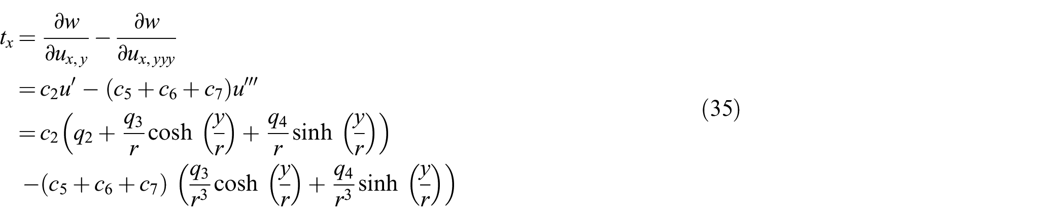
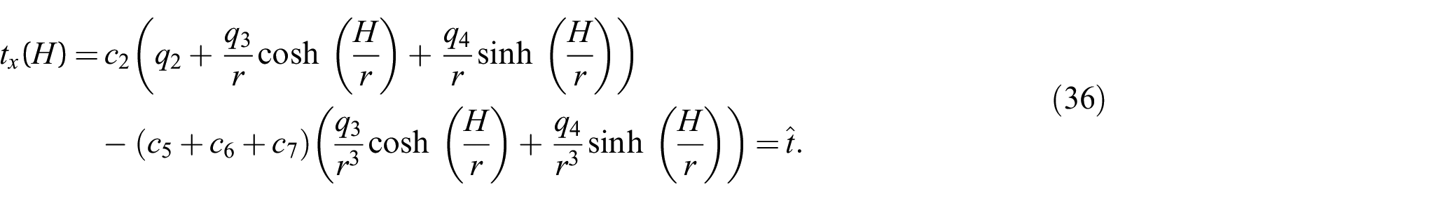
The double traction, $m_{\mathrm{xy}}$ , has been defined in equation (11) and is calculated in equation (21). For the current problem, the double traction has only one non-zero term as

$$\begin{array}{cc}\multicolumn{1}{c}{m_{\mathrm{xy}}=}& \frac{\partial w}{\partial u_{x,\mathrm{yy}}}=(c_5+c_6+c_7)u″\hfill \\ \multicolumn{1}{c}{}& =(c_5+c_6+c_7)(\frac{q_3}{r^2}\sinh \left(\frac{y}{r}\right)+\frac{q_4}{r^2}\cosh \left(\frac{y}{r}\right)).\hfill \end{array}$$

(29)

Therefore, for the third boundary condition in equation (26), we have

$$m_{\mathrm{xy}}\left(0\right)=(c_5+c_6+c_7)u″\left(0\right)=(c_5+c_6+c_7)\frac{q_4}{r^2}=0,$$

(30)

and for the fourth boundary condition, we take the derivative of $u$ in equation (25) with respect to $y$ , and set $y=H$ ,

$$u\prime \left(H\right)=q_2+\frac{q_3}{r}\cosh \left(\frac{H}{r}\right)+\frac{q_4}{r}\sinh \left(\frac{H}{r}\right)=0.$$

(31)

By solving equations (27), (28), (30), and (31), as shown in Appendix 2, the four unknowns $(q_1,q_2,q_3,q_4)$ are acquired

$$\begin{array}{cc}\multicolumn{1}{c}{}& q_1=0,q_2=\frac{\hat{u}\cosh \left(\frac{H}{r}\right)}{H\cosh \left(\frac{H}{r}\right)-r\sinh \left(\frac{H}{r}\right)},\hfill \\ \multicolumn{1}{c}{}& q_3=\frac{\hat{u}r}{r\sinh \left(\frac{H}{r}\right)-H\cosh \left(\frac{H}{r}\right)},q_4=0.\hfill \end{array}$$

(32)

3.2. Case 2: applying traction

In the second case, as shown in Figure 2, the boundary conditions are considered as

$$u_x\left(0\right)=0,t_x\left(H\right)=\hat{t},u\prime \left(0\right)=0,m_{\mathrm{xy}}\left(H\right)=0,$$

(33)

where a Neumann boundary condition is assumed on the top edge by a given traction $\hat{t}$ (as defined in equation (10)). The double traction is set to zero on the top edge. Furthermore, the displacement and displacement gradient are set to zero on the bottom edge. The latter condition is responsible for the strain gradient terms of the theory. Indeed, it models a clamped edge as seen in Figure 2.

For the first boundary condition in equation (33), from equation (25), we obtain

$$u_x\left(0\right)=q_1+q_4=0.$$

(34)

The traction, $t_x$ with $n=(0,1)$ , has been defined in equation (10), and for the current problem, it is reduced to

$$\begin{array}{cc}\multicolumn{1}{c}{t_x=}& \frac{\partial w}{\partial u_{x,y}}-\frac{\partial w}{\partial u_{x,\mathrm{yyy}}}\hfill \\ \multicolumn{1}{c}{=}& c_{2}u\prime -(c_5+c_6+c_7)u″\prime \hfill \\ \multicolumn{1}{c}{=}& c_2(q_2+\frac{q_3}{r}\cosh \left(\frac{y}{r}\right)+\frac{q_4}{r}\sinh \left(\frac{y}{r}\right))\hfill \\ \multicolumn{1}{c}{-}& (c_5+c_6+c_7)(\frac{q_3}{r^3}\cosh \left(\frac{y}{r}\right)+\frac{q_4}{r^3}\sinh \left(\frac{y}{r}\right))\hfill \end{array}$$

(35)

Therefore, for the second boundary condition in equation (33), we have

$$\begin{array}{cc}\multicolumn{1}{c}{}& t_x\left(H\right)=c_2(q_2+\frac{q_3}{r}\cosh \left(\frac{H}{r}\right)+\frac{q_4}{r}\sinh \left(\frac{H}{r}\right))\hfill \\ \multicolumn{1}{c}{}& -(c_5+c_6+c_7)(\frac{q_3}{r^3}\cosh \left(\frac{H}{r}\right)+\frac{q_4}{r^3}\sinh \left(\frac{H}{r}\right))=\hat{t}.\hfill \end{array}$$

(36)

The third and fourth boundary conditions in equation (33) give

$$m_{\mathrm{xy}}\left(H\right)=(c_5+c_6+c_7)(\frac{q_3}{r^2}\sinh \left(\frac{H}{r}\right)+\frac{q_4}{r^2}\cosh \left(\frac{H}{r}\right))=0,$$

(37)

and

$$u\prime \left(0\right)=q_2+\frac{q_3}{r}=0,$$

(38)

respectively.

By solving equations (34), (36), (37), and (38), as shown in Appendix 3, the four unknowns $(q_1,q_2,q_3,q_4)$ are obtained as

$$\begin{array}{cc}\multicolumn{1}{c}{}& q_1=\frac{-r^3\hat{t}\sinh \left(\frac{H}{r}\right)}{s},q_2=\frac{r^2\hat{t}\cosh \left(\frac{H}{r}\right)}{s},\hfill \\ \multicolumn{1}{c}{}& q_3=\frac{-r^3\hat{t}\cosh \left(\frac{H}{r}\right)}{s},q_4=\frac{r^3\hat{t}\sinh \left(\frac{H}{r}\right)}{s},\hfill \end{array}$$

(39)

where

$$s=c_2{r}^2(\cosh \left(\frac{H}{r}\right)-1)+c_5+c_6+c_7.$$

(40)

4. Numerical implementation

For the numerical implementation of the strain gradient theory, we use the same simple shear problem as in the analytical solution. Two approaches are discussed in the following: (1) FEM and (2) Mixed FEM. The modeling, implementation, and post-processing steps are all carried out using open-source packages. For the FEM analysis, we utilize the FEniCS libraries (73) by following the computational framework as in Abali (74). FEniCS is a package of codes for solving partial differential equations, and it supports symbolic differentiation, which is exploited herein. The FEM code is developed in Python.

The plate under simple shear is modeled as a two-dimensional plate with the height $H=0.5$ mm. In the problem description, the length of the plate is assumed to be infinite in the $x$ -direction. In the numerical models, we set a finite value for the length (three times of the height of the plate). Periodic boundary conditions are applied on the lateral edges of the plates; hence, the results will not depend on the value that is chosen for the plate’s length. The periodic boundary conditions applied on the left and right edges of the plate impose the following conditions on the domain: (1) the left and right edges of the plate are of course equal in length, (2) the nodes of these two edges have the same vertical coordinates such that there are corresponding nodes on both edges, and (3) the nodal value at the left is restricted to be the same as the corresponding nodal value at the right.

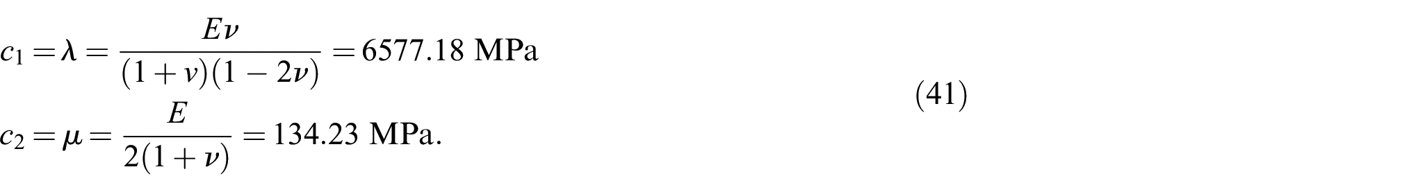
For the material of the plate, we assume Young’s modulus, $E=400$ MPa and Poisson’s ratio, $\nu =0.49$ . The choice of Poisson’s ratio is crucial for consistency with the semi-analytical ansatz. The simple shear problem is valid under the constant volume assumption that is equivalent to a Poisson’s ratio of 0.5, but here it is not possible to use 0.5 value since it makes the first Lame parameter $\left(c_1\right)$ to be infinite; therefore, we use 0.49 for Poisson’s ratio. The constitutive parameters $c_1$ and $c_2$ read

$$\begin{array}{cc}\multicolumn{1}{c}{}& c_1=\lambda =\frac{E\nu }{(1+v)(1-2\nu )}=6577.18\mathrm{MPa}\hfill \\ \multicolumn{1}{c}{}& c_2=\mu =\frac{E}{2(1+\nu )}=134.23\mathrm{MPa}.\hfill \end{array}$$

(41)

Moreover, the material parameters for strain gradient elasticity need to be chosen. For this purpose, herein, we utilize the granular micromechanical modeling [75–78]. Based on the formulation derived in Barchiesi et al. [79], we have

$$\begin{array}{cc}\multicolumn{1}{c}{}& c_3=c_4=\frac{{\ell }^2}{112}\lambda \hfill \\ \multicolumn{1}{c}{}& c_5=c_7=\frac{{\ell }^2}{1120}(7\mu +3\lambda )\hfill \\ \multicolumn{1}{c}{}& c_6=\frac{{\ell }^2}{1120}(7\mu -4\lambda ),\hfill \end{array}$$

(42)

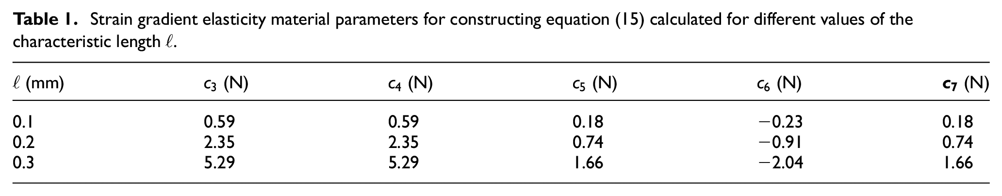
where $\ell$ is the characteristic length of the granular material of the substructure. We assume three values for $\ell$ as $\{0.1,0.2,0.3\}$ mm, which lead to material parameters as compiled in Table 1. The negative values in Table 1 may raise concern about the positive definiteness of the strain energy function. However, the individual values of the material parameters are not of importance. The energy value must be indeed positive in order to have a unique solution. We refer to previous studies [66,70,80] for discussion of positive definiteness in the strain gradient theory. In the problem Case 1, we set $\hat{u}=0.05$ mm and in the problem Case 2, we set $\hat{t}=1.0$ MPa.

Table 1.

Strain gradient elasticity material parameters for constructing equation (15) calculated for different values of the characteristic length $\ell$ .

$\ell$ (mm)	$c_3$ (N)	$c_4$ (N)	$c_5$ (N)	$c_6$ (N)	${\mathit{c}}_7$ (N)
0.1	0.59	0.59	0.18	−0.23	0.18
0.2	2.35	2.35	0.74	−0.91	0.74
0.3	5.29	5.29	1.66	−2.04	1.66

4.1. FEM

In the classical elasticity theory, we deal with a second-order partial differential equation, while in the strain gradient elasticity theory, we have a governing equation of fourth order [81]. As a result, for satisfying the ${\mathcal{H}}^2$ regularity in the weak form, unknown fields need to belong to $C^1$ within the whole domain. One possible approach is to set the minimum regularity requirement for the shape functions to be $C^1$ [82,83]. Another implementation of the strain gradient theory with $C^1$ regularity is presented in Glüge [51].

For obtaining the weak form for implementing in the FEM code, we begin with the governing equation of strain gradient elasticity as derived in equation (7). The unknown displacement $u_i$ is represented using nodal values discretely in space and form functions for interpolation between nodal values. We circumvent using different notations for analytical functions and their discrete representations, since they never appear in the same equation. We use a discretization using (triangle) Lagrange elements, which generates piecewise continuous polynomials such that they are adequate for approximation in Hilbertian Sobolev space ${\mathcal{H}}^1$ . This standard FEM elements of order $q$ spans ${\mathcal{P}}_q$ on triangles, $T$ , in a two-dimensional continuum. The computational domain, $\mathrm{\Omega }$ , is discretized by dividing it in triangles, and this triangulation is denoted by $\mathcal{T}$ . Therefore, we use a vector space for displacements

$$\begin{array}{c}{\mathcal{V}}_{\mathrm{FEM}}=\{{\left\{u_i\right\}\in {\mathcal{H}}^1\left(\mathrm{\Omega }\right):\left\{u_i\right\}|}_T\in {\mathcal{P}}_2(T)\forall T\in \mathcal{T}\}.\hfill \end{array}$$

(43)

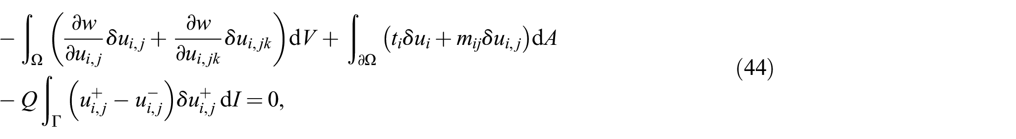
The Lagrange elements are $C^0$ continuous across element boundaries; however, it is necessary to have $C^1$ continuity everywhere in the domain. Instead of using more advanced elements [84], we add a term to the weak form to enforce the continuity of the first gradient of displacement across the elements. By adding such a term to equation (7), we obtain

$$\begin{array}{cc}\multicolumn{1}{c}{}& -{\int }_{\mathrm{\Omega }}(\frac{\partial w}{\partial u_{i,j}}\delta u_{i,j}+\frac{\partial w}{\partial u_{i,\mathrm{jk}}}\delta u_{i,\mathrm{jk}})\mathrm{d}V+{\int }_{\partial \mathrm{\Omega }}(t_i\delta u_i+m_{\mathrm{ij}}\delta u_{i,j})\mathrm{d}A\hfill \\ \multicolumn{1}{c}{}& -Q{\int }_{\Gamma }(u_{i,j}^{+}-u_{i,j}^{-})\delta u_{i,j}^{+}\mathrm{d}I=0,\hfill \end{array}$$

(44)

where

$$Q=\sqrt{c_2(c_5+c_6+c_7)},$$

(45)

and we have inserted $\frac{\partial W_s}{\partial u_i}=t_i$ and $\frac{\partial W_s}{\partial u_{i,j}}=m_{\mathrm{ij}}$ from equations (10) and (11), respectively. The term $Q$ is the penalty parameter; it is chosen arbitrarily but in connection with the material parameters and in the adequate unit in a way that all the terms in equation (44) have the same unit. Since the formulation involves second gradient in space, we choose $q=2$ such that ${\mathcal{P}}_2$ elements are utilized.

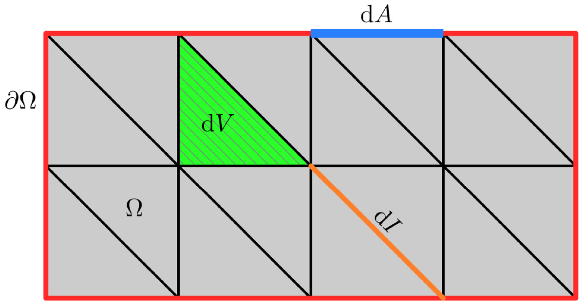
In equation (44), $u_{i,j}^{+}$ and $u_{i,j}^{-}$ are the displacement gradients on the two sides of an interior facet, which is between pairs of adjacent cells of the mesh. Moreover, the integration in $\mathrm{d}I$ is done on the set $\Gamma$ of the two-sided facet elements while $\mathrm{d}A$ is for the one-sided exterior facets of the mesh, i.e., belonging the boundaries of the domain. Figure 3 shows a schematic of a triangular mesh on a domain $\mathrm{\Omega }$ , its boundary $\partial \mathrm{\Omega }$ , a cell element $\mathrm{d}V$ , a one-sided exterior facet element $\mathrm{d}A$ , and a two-sided facet (edge) element $\mathrm{d}I$ . The formulation holds in two-dimensional or three-dimensional domains; however, for the sake of the visualization, we show the idea on a two-dimensional mesh in Figure 3. In a two-dimensional domain, which is the case herein, the cell element $\mathrm{d}V$ is a surface and the facets $\mathrm{d}A$ and $\mathrm{d}I$ are edge elements.

Figure 3.

Schematic of a triangular mesh on a domain $\mathrm{\Omega }$ , its boundary $\partial \mathrm{\Omega }$ , a cell (surface) element $\mathrm{d}V$ , a one-sided exterior facet (edge) element $\mathrm{d}A$ , and a two-sided facet (edge) element $\mathrm{d}I$ .

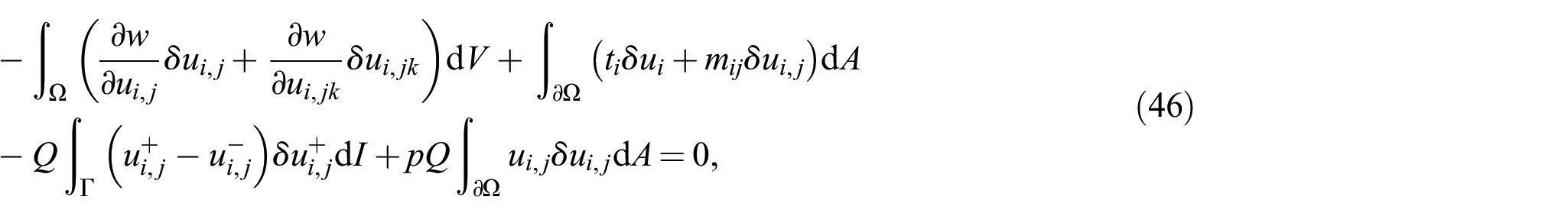
It is possible to add a displacement prescription in the numerical computations as a Dirichlet boundary condition. However, in the problems that are discussed in the analytical solution (Section 3), there are boundary conditions of “zero-displacement gradient” on top (Case 1) and bottom (Case 2) edges of the rectangular domain. It is not possible to add such a boundary condition directly in the numerical computations. Hence, we add the zero-displacement gradient condition into the weak form. We update the weak form of equation (44) as

$$\begin{array}{cc}\multicolumn{1}{c}{}& -{\int }_{\mathrm{\Omega }}(\frac{\partial w}{\partial u_{i,j}}\delta u_{i,j}+\frac{\partial w}{\partial u_{i,\mathrm{jk}}}\delta u_{i,\mathrm{jk}})\mathrm{d}V+{\int }_{\partial \mathrm{\Omega }}(t_i\delta u_i+m_{\mathrm{ij}}\delta u_{i,j})\mathrm{d}A\hfill \\ \multicolumn{1}{c}{}& -Q{\int }_{\Gamma }(u_{i,j}^{+}-u_{i,j}^{-})\delta u_{i,j}^{+}\mathrm{d}I+\mathrm{pQ}{\int }_{\partial \mathrm{\Omega }}{u}_{i,j}\delta u_{i,j}\mathrm{d}A=0,\hfill \end{array}$$

(46)

where $p={10}^6$ is a penalty factor. Here, the last integral of equation (46) enforces the gradient of displacement to be zero on the intended boundary (top or bottom edge of the plate). For the problem of Case 1 (Section 3.1), we set $t_i=0$ and $m_{\mathrm{ij}}=0$ in the weak form (46) as there are no traction or double traction applied on the boundaries. Furthermore, the last integral of the weak form is calculated on the top edge of the domain $(y=H)$ . For the problem of Case 2 (Section 3.2), we set $t_i=\hat{t}$ and $m_{\mathrm{ij}}=0$ in the weak form (46) as the traction $\hat{t}$ is applied on the top edge of the domain and there is no double traction applied on the boundaries. Moreover, the last integral of the weak form is calculated on the bottom edge of the domain $(y=0)$ .

4.2. Mixed FEM

The Mixed FEM is developed using the Hu–Washizu principle [85]. In the Mixed FEM, more than one function space is used for approximating the variables. Each function space is dedicated to one of the variables, and all the variables are solved simultaneously. In other words, the additional variables are calculated independently together with the primitive variable.

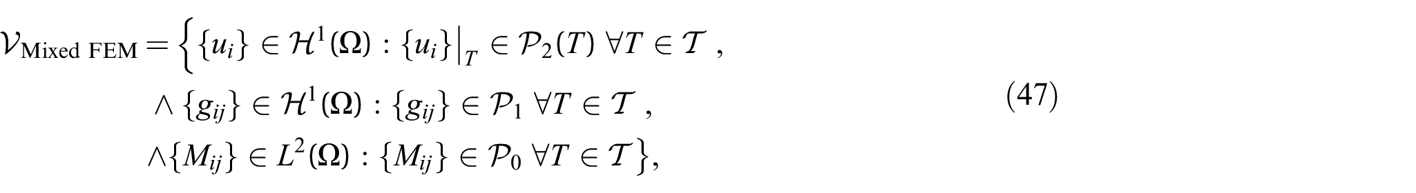
Herein, we define three function spaces in the Mixed FEM formulation, which involves $\{u_i,g_{\mathrm{ij}},M_{\mathrm{ij}}\}$ . The first one (Space 1) is a vector space for the primitive variable of the problem, the displacement $u_i$ , for which we choose $q=2$ and ${\mathcal{P}}_2$ (quadratic) shape functions. We use a distinct notation for the space derivatives in order to clearly approximate the space derivative of displacement. As the second space in the mixed formulation (Space 2), we introduce $g_{\mathrm{ij}}=u_{i,j}$ as a variable to be identified in the computations. We use ${\mathcal{P}}_1$ (linear) shape functions for the unknown $g_{\mathrm{ij}}$ . For the spaces of displacement and displacement gradient, we use standard polynomial FEM elements in FEniCS.

Then, we impose $u_{i,j}=g_{\mathrm{ij}}$ in the computations. This condition ensures that the approximated $g_{\mathrm{ij}}$ in Space 2 is equal to the gradient of the approximated displacement in Space 1. For enforcing such an identity condition, as we will explain in the following, we define a tensor space of Lagrange multipliers, $M_{\mathrm{ij}}$ . We choose $L^2$ elements for $M_{\mathrm{ij}}$ with ${\mathcal{P}}_0$ such that they are simply constants within elements with a jump across boundaries. We choose the family of discontinuous Galerkin elements in FEniCS which are suitable for this purpose. We set the degree of element to zero as we need constant functions.

At the end, we have the three unknown functions $\{u_i,g_{\mathrm{ij}},M_{\mathrm{ij}}\}$ . For our two-dimensional problem, in each node, there are 2 unknowns for the components of $u_i$ , 4 unknowns for $g_{\mathrm{ij}}$ , and 4 unknowns for $M_{\mathrm{ij}}$ , i.e., 10 unknowns in total. These 10 unknowns are all independent in the formulation. In a nutshell, we construct the space for the Mixed FEM formulation as

$$\begin{array}{cc}\multicolumn{1}{c}{}& {\mathcal{V}}_{\mathrm{Mixed}\mathrm{FEM}}=\{{\left\{u_i\right\}\in {\mathcal{H}}^1\left(\mathrm{\Omega }\right):\left\{u_i\right\}|}_T\in {\mathcal{P}}_2(T)\forall T\in \mathcal{T},\hfill \\ \multicolumn{1}{c}{}& \wedge \left\{g_{\mathrm{ij}}\right\}\in {\mathcal{H}}^1\left(\mathrm{\Omega }\right):\left\{g_{\mathrm{ij}}\right\}\in {\mathcal{P}}_1\forall T\in \mathcal{T},\hfill \\ \multicolumn{1}{c}{}& \wedge \left\{M_{\mathrm{ij}}\right\}\in L^2\left(\mathrm{\Omega }\right):\left\{M_{\mathrm{ij}}\right\}\in {\mathcal{P}}_0\forall T\in \mathcal{T}\},\hfill \end{array}$$

(47)

within the domain of the continuum body, $\mathrm{\Omega }$ , with its closure, $\partial \mathrm{\Omega }$ , where boundary values are given on Dirichlet boundaries, $\partial {\mathrm{\Omega }}_D$ .

In the Mixed FEM formulation, we create one single mesh in the domain and each of the function spaces is constructed on the same mesh. Depending on the dimension, degree of shape function, and element type, each space has a different total number of degrees of freedom in the domain. The quadratic vector space of $u_i$ has 21,960, the linear tensor space of $g_{\mathrm{ij}}$ has 11,160, and the scalar tensor space of $M_{\mathrm{ij}}$ has 21,600 degrees of freedom. In total, the mixed space has 54,720 degrees of freedom. The test functions, $\delta u_i,\delta g_{\mathrm{ij}},\delta M_{\mathrm{ij}}$ , are chosen from the same space as the $u_i,g_{\mathrm{ij}},M_{\mathrm{ij}}$ , respectively.

For generating the weak form for the Mixed FEM approach, we begin with the governing equation of equation (7). From equations (18) and (19), we have

$$\frac{\partial w}{\partial u_{i,j}}=C_{\mathrm{ijkl}}{\epsilon }_{\mathrm{kl}},\frac{\partial w}{\partial u_{i,\mathrm{jk}}}=D_{\mathrm{ijklmn}}{\epsilon }_{\mathrm{lm},n}.$$

(48)

By inserting $\frac{\partial w}{\partial u_{i,j}}$ and $\frac{\partial w}{\partial u_{i,\mathrm{jk}}}$ in equation (7), and also setting $\frac{\partial W_s}{\partial u_i}=t_i$ and $\frac{\partial W_s}{\partial u_{i,j}}=m_{\mathrm{ij}}$ from equations (10) and (11), respectively, we obtain

$${\int }_{\mathrm{\Omega }}(C_{\mathrm{ijkl}}{\epsilon }_{\mathrm{kl}}\delta u_{i,j}+D_{\mathrm{ijklmn}}{\epsilon }_{\mathrm{lm},n}\delta g_{\mathrm{ij},k})\mathrm{d}V-{\int }_{\partial \mathrm{\Omega }}(t_i\delta u_i+m_{\mathrm{ij}}\delta u_{i,j})\mathrm{d}A=0,$$

(49)

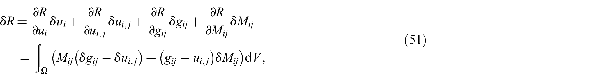
where we have replaced the $\delta u_{i,\mathrm{jk}}$ with $\delta g_{\mathrm{ij},k}$ since it is the test function related to the second gradient of displacement. For imposing the identity $u_{i,j}=g_{\mathrm{ij}}$ (the equality of the approximated $g_{\mathrm{ij}}$ in Space 2 and the gradient of the approximated displacement in Space 1), we define a residual as

$$R={\int }_{\mathrm{\Omega }}{M}_{\mathrm{ij}}(g_{\mathrm{ij}}-u_{i,j})\mathrm{d}V.$$

(50)

Taking the variation of $R$ gives

$$\begin{array}{cc}\multicolumn{1}{c}{}& \delta R=\frac{\partial R}{\partial u_i}\delta u_i+\frac{\partial R}{\partial u_{i,j}}\delta u_{i,j}+\frac{\partial R}{\partial g_{\mathrm{ij}}}\delta g_{\mathrm{ij}}+\frac{\partial R}{\partial M_{\mathrm{ij}}}\delta M_{\mathrm{ij}}\hfill \\ \multicolumn{1}{c}{}& ={\int }_{\mathrm{\Omega }}(M_{\mathrm{ij}}(\delta g_{\mathrm{ij}}-\delta u_{i,j})+(g_{\mathrm{ij}}-u_{i,j})\delta M_{\mathrm{ij}})\mathrm{d}V,\hfill \end{array}$$

(51)

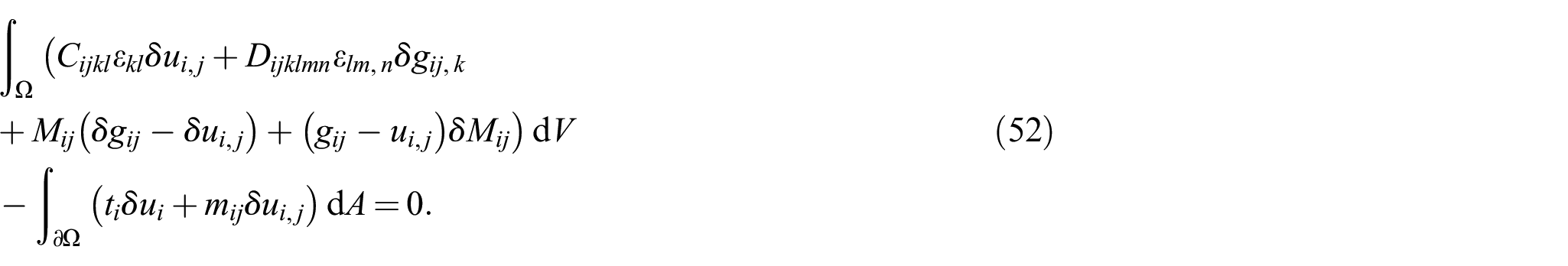
which should vanish in the domain $\mathrm{\Omega }$ as we aim at minimizing the residual $R$ . The complete weak form of the Mixed FEM approach is generated by adding the variation of $R$ from equation (51) to equation (49) as

$$\begin{array}{cc}\multicolumn{1}{c}{}& {\int }_{\mathrm{\Omega }}(C_{\mathrm{ijkl}}{\epsilon }_{\mathrm{kl}}\delta u_{i,j}+D_{\mathrm{ijklmn}}{\epsilon }_{\mathrm{lm},n}\delta g_{\mathrm{ij},k}\hfill \\ \multicolumn{1}{c}{}& +M_{\mathrm{ij}}(\delta g_{\mathrm{ij}}-\delta u_{i,j})+(g_{\mathrm{ij}}-u_{i,j})\delta M_{\mathrm{ij}})\mathrm{d}V\hfill \\ \multicolumn{1}{c}{}& -{\int }_{\partial \mathrm{\Omega }}(t_i\delta u_i+m_{\mathrm{ij}}\delta u_{i,j})\mathrm{d}A=0.\hfill \end{array}$$

(52)

For the problem of Case 1 (Section 3.1), we set $t_i=0$ and $m_{\mathrm{ij}}=0$ in the weak form (52) as there are no traction or double traction applied on the boundaries. For the problem of Case 2 (Section 3.2), we set $t_i=\hat{t}$ and $m_{\mathrm{ij}}=0$ in the weak form (52) as the traction $\hat{t}$ is applied on the top edge of the domain and there is no double traction applied on the boundaries. The zero gradient boundary conditions of the problem Cases 1 and 2 are applied as Dirichlet boundary conditions.

5. Results and discussion

In this section, the results of the computations are presented and verified by comparing them with the analytical solutions. Furthermore, the convergence analyses of the formulations are reported.

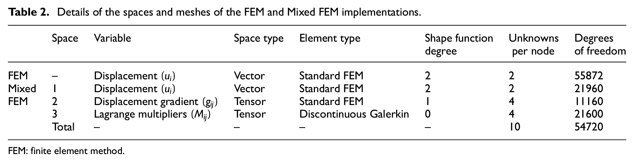
As discussed in Section 4, two numerical implementations are used for the computations: FEM and Mixed FEM. Table 2 summarizes the details of the spaces and the meshes of the two implementations. As shown in Table 2, the total degrees of freedom in the two implementations are of the same order since we want to compare their accuracy.

Table 2.

Details of the spaces and meshes of the FEM and Mixed FEM implementations.

	Space	Variable	Space type	Element type	Shape function degree	Unknowns per node	Degrees of freedom
FEM	–	Displacement $\left(u_i\right)$	Vector	Standard FEM	2	2	55872
Mixed FEM	1	Displacement $\left(u_i\right)$	Vector	Standard FEM	2	2	21960
	2	Displacement gradient $\left(g_{\mathrm{ij}}\right)$	Tensor	Standard FEM	1	4	11160
	3	Lagrange multipliers $\left(M_{\mathrm{ij}}\right)$	Tensor	Discontinuous Galerkin	0	4	21600
	Total	–	–	–	–	10	54720

FEM: finite element method.

5.1. Results of Case 1

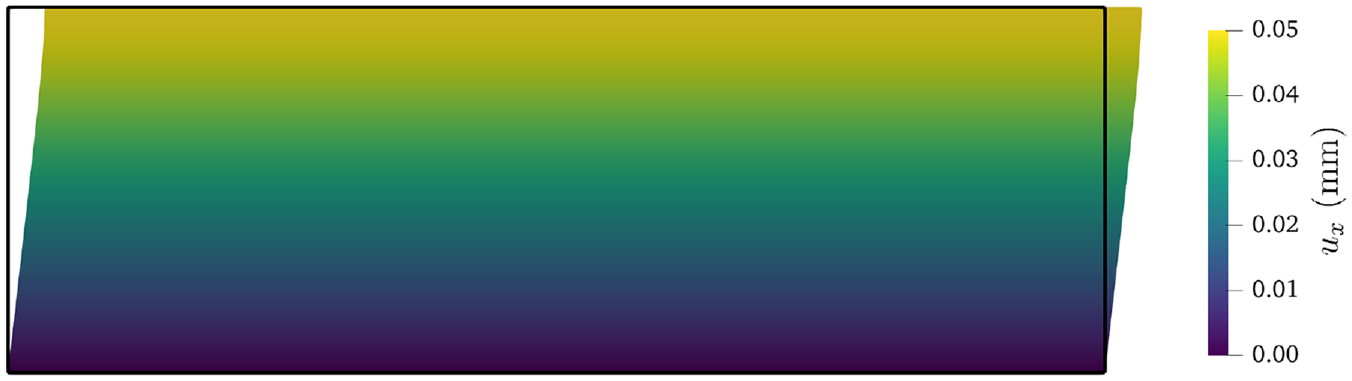
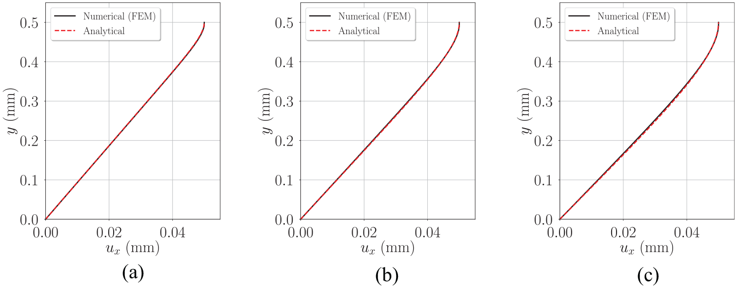
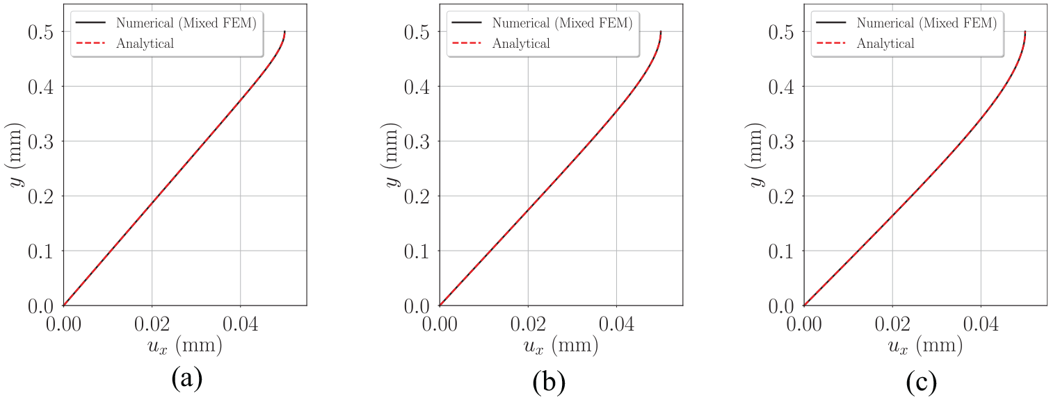
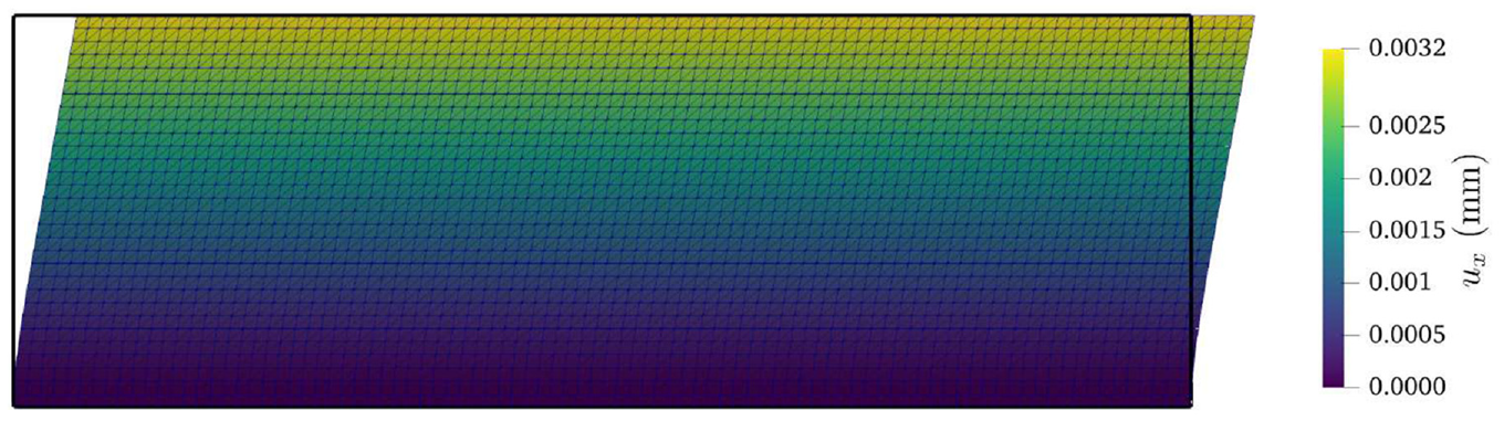
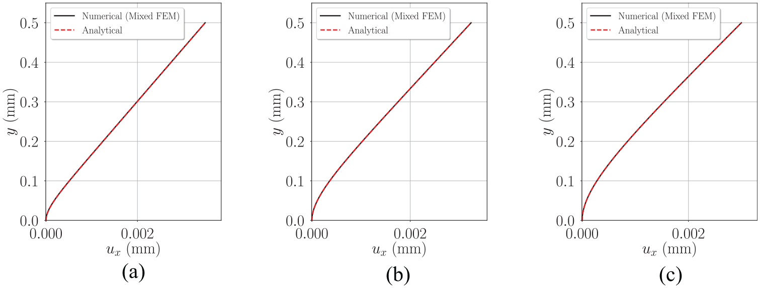
Figure 4 shows the deformed state of the plate that has been under prescribed displacement on the top edge from FEM analysis. The effect of the zero-displacement gradient condition on the top edge $(u\prime (H)=0)$ is visible in this plot. We see that the lateral edges of the plate are fully vertical in the very beginning of their upper part. In order to compare the numerical and analytical results, we consider the displacement of the right edge of the plate. The displacement $\left(u_x\right)$ of the right edge calculated by FEM and Mixed FEM is plotted along $y$ in Figures 5 and 6, respectively, for three values of the characteristic length, $\ell$ , which results in different material parameters, $c_3,c_4,c_5,c_6,\mathrm{and}{c}_7$ . Figures 5 and 6 show that both FEM and Mixed FEM formulations are matching in a very satisfactory way with the analytical solution.

Figure 4.

The deformed state of the plate under prescribed displacement on the top edge (Case 1) from FEM analysis.

Figure 5.

Displacement of the right edge of the plate, under prescribed displacement on the top edge (Case 1), along $y$ : numerical computation (FEM) versus analytical solution for three different values of $\ell$ : (a) $\ell =0.1$ mm, (b) $\ell =0.2$ mm, and (c) $\ell =0.3$ mm.

Figure 6.

Displacement of the right edge of the plate, under prescribed displacement on the top edge (Case 1), along $y$ : numerical computation (Mixed FEM) vs analytical solution for three different values of $\ell$ : (a) $\ell =0.1$ mm, (b) $\ell =0.2$ mm, and (c) $\ell =0.3$ mm.

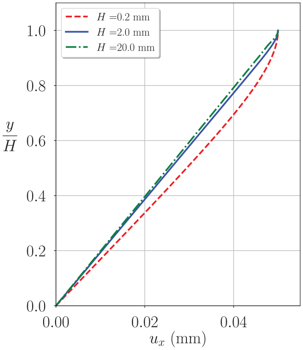
To see the role of strain gradient terms in systems with different sizes, we simulate the problem of Case 1 for three plates using the Mixed FEM formulation. The height of the three plates are $H=\{0.2,2.0,20.0\}$ mm. We set the characteristic length, $\ell =0.1$ mm, and prescribed displacement, $\hat{u}=0.05$ mm, for the three simulations. Figure 7 shows the displacement of right edge along $y$ normalized with respect to plate height. We see, in Figure 7, that the $H=20.0$ mm case is behaving linearly compared to the smaller heights. The reason is simply the increased ratio of the characteristic length of the geometry, $H$ , by the characteristic length of the material, $\ell$ . As expected, for higher $H/\ell$ values, strain gradient terms are less important. In fact, the strain gradient theory is necessary between $H/\ell$ larger than 1 and smaller than a certain value which can be estimated using the study presented herein.

Figure 7.

Displacement of the right edge of the plate, under prescribed displacement on the top edge (Case 1) from Mixed FEM analysis for different values of plate height, $H$ , and $\ell =0.1$ mm.

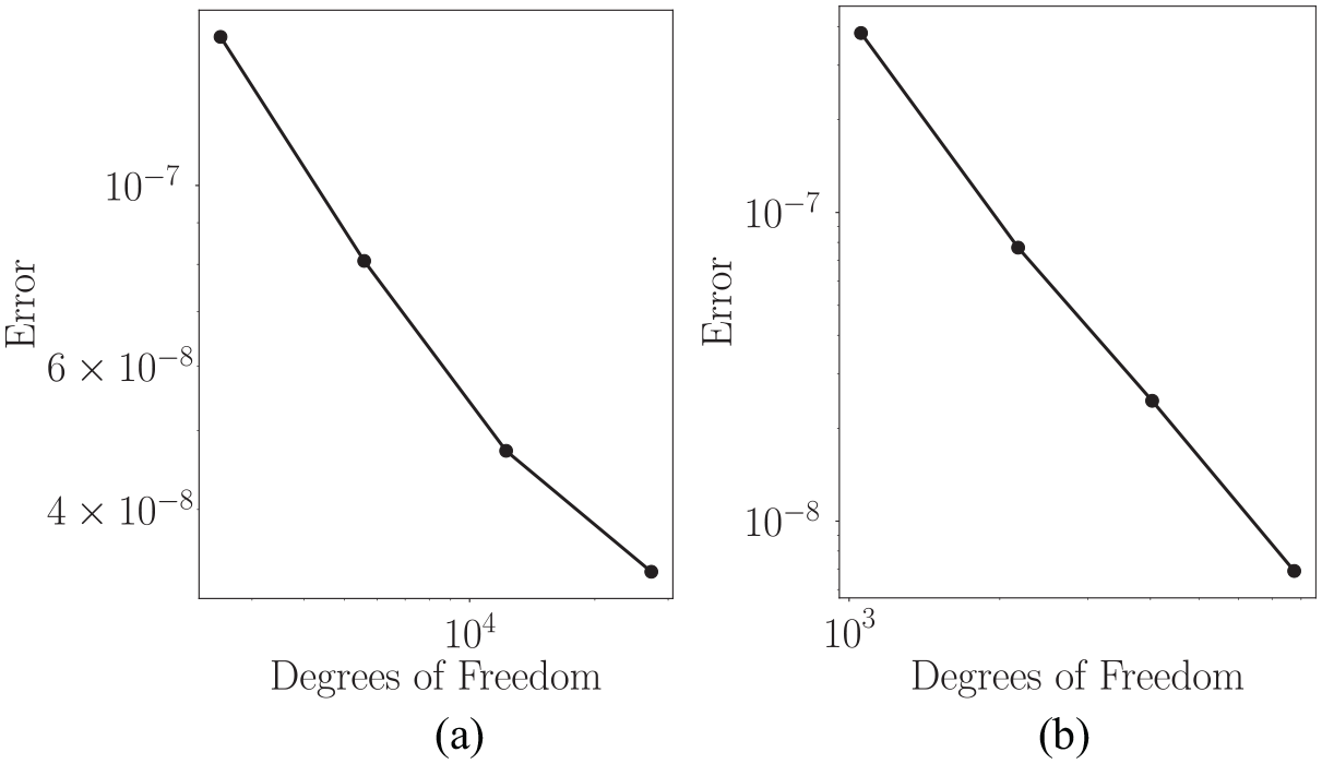
Convergence analyses are carried out for the FEM and Mixed FEM implementations to ensure the mesh independency of the results. The error is defined as

$$\mathrm{Error}={\int }_{\mathrm{\Omega }}|u_i^{\mathrm{comp}}-u_i^{\mathrm{ana}}{|}^2\mathrm{d}V$$

(53)

where $u_i^{\mathrm{comp}}$ is the displacement from the numerical analysis and $u_i^{\mathrm{ana}}$ is the displacement from the analytical solution. In Figure 8(a) and (b), the monotonously decreasing trend of the error on the $\log -\log$ plots is seen for FEM and Mixed FEM implementations, respectively.

Figure 8.

Mesh convergence analysis of FEM and Mixed FEM approaches in log-log scale: (a) FEM and (b) Mixed FEM.

5.2. Results of Case 2

In the problem of Case 2, a traction is applied on the top edge of the plate. Figure 9 depicts the deformation of the plate from Mixed FEM analysis. Here, we see the effect of the zero-displacement gradient condition on the bottom edge $(u\prime (0)=0)$ . As a result, the lateral edges of the plate are vertical in the very lower part. For Case 2, the FEM formulation does not produce reliable results and it is not verified by the analytical solution. On the contrary, the Mixed FEM formulation yields highly matching results with the analytical solutions. Figure 10 shows the displacement $\left(u_x\right)$ of the right edge calculated by Mixed FEM for three values of the characteristic length, $\ell$ , which results in different values for the material parameters, $c_3,c_4,c_5,c_6,\mathrm{and}{c}_7$ .

Figure 9.

The deformed state of the plate under applied traction on the top edge (Case 2) from Mixed FEM analysis (Deformation scale: 25:1).

Figure 10.

Displacement of the right edge of the plate, under applied traction on the top edge (Case 2), along $y$ : numerical computation (Mixed FEM) vs analytical solution for three different values of $\ell$ . (a) $\ell =0.1$ mm, (b) $\ell =0.2$ mm, and (c) $\ell =0.3$ mm.

6. Conclusion

Two implementations of the strain gradient elasticity theory based on the FEM are verified. The governing equation of the strain gradient elasticity is modeled using FEM and Mixed FEM, in which three distinct function spaces for the different variables are introduced, allowing the simultaneous determination of the different unknowns on the three distinct spaces. For a simple shear problem, the computations are verified with an analytical solution. The Mixed FEM proved to be reliable in the considered boundary conditions (applying traction and displacement) while the FEM approach succeeds in predicting the displacement only in one of the cases of boundary conditions.

In the FEM implementation approach, in every node, there exist 2 degrees of freedom, while in the Mixed FEM, the number of degrees of freedom is 10 per node; however, for FEM computations, a finer mesh is necessary to give acceptable results. In a nutshell, the Mixed FEM formulation proves to be more robust and reliable for solving problems in the framework of the strain gradient elasticity theory. The codes used for the computations are developed under the GNU Public license [86] made publicly available in Abali [87] for encouraging a transparent scientific exchange.