Sage Journals: Discover world-class research

Abstract

The study of periodic systems under the action of moving loads is of high practical importance in railway, road, and bridge engineering, among others. Even though plenty of studies focus on periodic systems, few of them are dedicated to the influence of a local inhomogeneous region, a so-called transition zone, on the dynamic response. In railway engineering, these transition zones are prone to significant degradation, leading to more maintenance requirements than the rest of the structure. This study aims to identify and investigate phenomena that arise due to the combination of periodicity and local inhomogeneity in a system acted upon by a moving load. To study such phenomena in their purest form, a one-dimensional model is formulated consisting of a constant moving load acting on an infinite string periodically supported by discrete springs and dashpots, with a finite domain in which the stiffness and damping of the supports is larger than for the rest of the infinite domain; this model is representative of a catenary system (overhead wires in railway tracks). The identified phenomena can be considered as additional constraints for the design parameters at transition zones such that dynamic amplifications are avoided.

Keywords

Periodic structure transition radiation moving load wave interference

1. Introduction

Periodic systems under the action of moving loads have attracted the attention of researchers in the past century. These problems pose academic challenges and are of high practical relevance due to their application in railway, road, and bridge engineering, among others. Despite the numerous studies on periodic systems, few investigations are dedicated to the influence of a local inhomogeneous region, a so-called transition zone, on the dynamic response. In railway engineering, significant degradation is observed in the vicinity of these transition zones, requiring more maintenance than the rest of the structure [1]. This study aims at investigating if the combination of (1) a transition zone and (2) the periodic nature of the structure can lead to undesired response amplification that is otherwise not observed in systems that neglect either (1) or (2).

The study of periodic structures goes back to Newton who investigated the velocity of sound in air using a lattice of point masses; for an interesting historical background of wave propagation in periodic lumped structures, see Brillouin [2]. Rayleigh studied for the first time a continuous periodic structure [3], considering a string with a periodic and continuous variation of density along its length. When it comes to a periodic and discrete variation in continuous structures, Mead [4 –6] was among the pioneers who studied free wave propagation in such systems. Concerning moving loads on such structures, Jezequel [7] and Cai et al. [8] were among the first to study periodically and discretely supported beams acted upon by a moving load. Vesnitskii and Metrikin [9,10] offered an extensive investigation into the behaviour of a periodically and discretely supported string acted upon by a moving load. More recently, there have been numerous studies of periodic guideways acted upon by vehicles, for example [11 –17], and also numerous studies focusing on the vehicle instability caused by the periodic nature of the guideway (i.e. parametric instability or sometimes called parametric resonance), for example [18,19].

Studies using complex models containing periodic structures and transition zones are present in literature, for example [20 –23]; however, these studies concentrate on predicting the transient response in the vicinity of the transition zone and do not treat specifically the influence of the discrete and periodic supports on these results. Moreover, with increased model complexity, the identification and investigation of particular/isolated phenomena becomes very difficult, if not impossible. Therefore, this paper focuses on the identification and investigation of specific phenomena that arise due to the combination of periodicity and local inhomogeneity in a system acted upon by a moving load. The local inhomogeneous region is itself periodic too, but with different parameters than the rest of the structure.

To study phenomena in their purest form, a one-dimensional (1D) model is formulated consisting of a constant moving load acting on an infinite string periodically supported by discrete springs and dashpots, with a finite domain in which the stiffness and damping of the supports is larger than for the rest of the infinite domain. The novelty of this research lies in the identification and investigation of three phenomena arising from the combination of periodicity and local inhomogeneity in a system acted upon by a moving load; they have not been yet reported in the literature. The three phenomena are described in detail in Sections 4.1, 4.2, and 4.3, respectively. Although these phenomena are identified in this simple model, they are intrinsic to any periodic system with a local inhomogeneity, and thus, can help understand the potential response amplification in more complex systems that incorporate these two characteristics. Finally, as this model is representative of a catenary system (overhead wires in railway tracks), the three identified phenomena can help understand the fatigue and wear of the catenary systems close to transition zones as well as wear in the energy collector system.

2. Model description

The system studied in this paper consists of an infinite string with distributed mass per unit length $ρ$ that is under tension $T$ ; the string is discretely supported by springs with stiffness $k_{s} (x)$ and dashpots with damping coefficient $c_{s} (x)$ ; the generic cell is defined at $x \in [nd, (n + 1) d]$ where $n$ is the cell number and $d$ is the cell width, and the spring-dashpot element is located in the middle of the cell at $x = \bar{n} d$ with $\bar{n} = n + \frac{1}{2}$ ; this system is acted upon by a moving constant load of amplitude $F_{0}$ and velocity $v$ . The stiffness and damping of the supports varies in space in such a way that there is a zone of length $l$ in which the stiffness and damping of the supports is $p$ times larger than for the rest of the infinite domain; the region in the close vicinity to the stiff zone is called the transition zone. Figure 1 presents a visual schematic of the system while its equation of motion reads

ρ \overset{\cdot\cdot}{w} - Tw ″ + \sum_{n = - \infty}^{\infty} (k_{s} (x) + c_{s} (x) \frac{\partial}{\partial t}) w δ (x - \bar{n} d) = - F_{0} δ (x - vt),

(1)

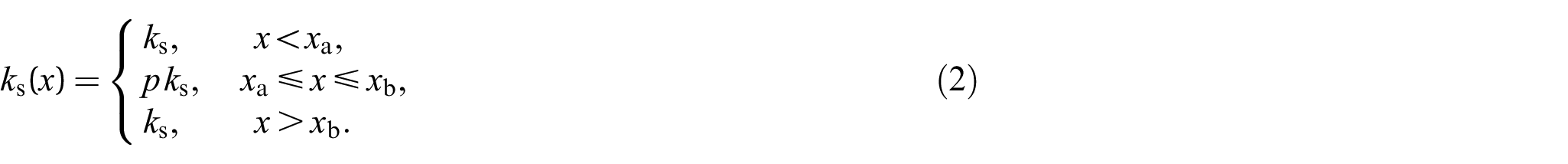
where primes and overdots denote partial derivatives in space and time, respectively. The supports stiffness is a piecewise function in space and is defined as follows:

k_{s} (x) = {\begin{matrix} k_{s}, x < x_{a}, \\ p k_{s}, x_{a} \leq x \leq x_{b}, \\ k_{s}, x > x_{b} . \end{matrix}

(2)

Figure 1.

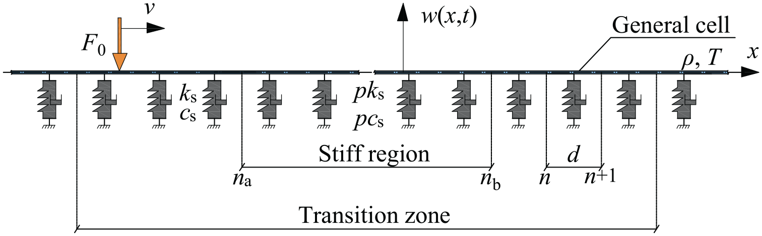
Model schematics: infinite tensioned string discretely supported by an inhomogeneous foundation, subjected to a moving constant load.

For simplicity, the spatial distribution of the damping is assumed to be the same as that of the stiffness. The values for the parameters are taken from Metrikine [24]; they represent the parameters for a realistic catenary system.

In the remainder of the paper, homogeneous system is used to refer to the system without transition zone while inhomogeneous system is used for the system with a transition zone, even though both systems are inherently inhomogeneous due to the discrete supports. Important to note, transition zone does not refer only to the stiff region, but to the stiff region and its vicinity, as can be seen in Figure 1.

3. Homogeneous system

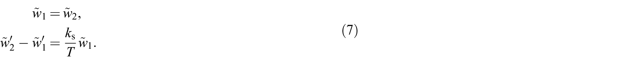
In this section, we present the characteristics of the periodic system without the transition zone. The goal here is to introduce the solution method used throughout this paper, to highlight important characteristics of the periodic and continuous system, and to present the steady-state response to a moving constant load. Note that the system without damping is considered here for clarity in the derivation. To this end, we aim at writing an expression linking the states (displacement and slope) at the two boundaries of a generic cell. First, we apply the forward Fourier transform over time to the equation of motion (equation (1)), thus obtaining the following expression:

\tilde{w} ″ + (\frac{ω^{2}}{c^{2}} - \sum_{n = - \infty}^{\infty} \frac{k_{s}}{T} δ (x - \bar{n} d)) \tilde{w} = \frac{F_{0}}{Tv} e^{- i ω \frac{x}{v}},

(3)

where the tilde is used to denote the quantity in the Fourier domain and $c = \sqrt{T / ρ}$ is the wave velocity in the unsupported string. We can limit our investigation to a generic cell $x \in [nd, (n + 1) d]$ and split this cell into two domains, with ${\tilde{w}}_{1}$ to the left of the support and ${\tilde{w}}_{2}$ to the right of it. This allows us to write the solutions in the two domains as follows:

{\tilde{w}}_{1} (x, ω) = C_{1} e^{- i γ x} + C_{2} e^{i γ x} + {\tilde{w}}_{p} (x, ω), nd \leq x \leq (n + \frac{1}{2}) d,

(4)

{\tilde{w}}_{2} (x, ω) = D_{1} e^{- i γ x} + D_{2} e^{i γ x} + {\tilde{w}}_{p} (x, ω), (n + \frac{1}{2}) d \leq x \leq (n + 1) d,

(5)

{\tilde{w}}_{p} (x, ω) = \frac{F_{0}}{T} \frac{v}{γ^{2} v^{2} - ω^{2}} e^{- i ω \frac{x}{v}},

(6)

where $γ = ω / c$ is the wavenumber in the unsupported string. Note that ${\tilde{w}}_{p}$ is the steady-state solution of an unsupported string acted upon by a moving constant load. The interface conditions between the two domains at $x = \bar{n} d$ represent displacement continuity and shear force equilibrium, and read.

\begin{matrix} {\tilde{w}}_{1} = {\tilde{w}}_{2}, \\ \tilde{w}'_{2} - \tilde{w}'_{1} = \frac{k_{s}}{T} {\tilde{w}}_{1} . \end{matrix}

(7)

Using the two interface conditions, $D_{1}$ and $D_{2}$ can be expressed in terms of $C_{1}$ and $C_{2}$ . Also, we express $C_{1}$ and $C_{2}$ in terms of the state at $x = nd$ (i.e. displacement ${\tilde{w}}_{n}$ and slope $\tilde{w}'_{n}$ ). The resulting state inside the generic cell reads

(\begin{matrix} \tilde{w} (x, ω) \\ \tilde{w}' (x, ω) \end{matrix}) = (\begin{matrix} f_{1, 1} (x - nd) & f_{1, 2} (x - nd) \\ f_{2, 1} (x - nd) & f_{2, 2} (x - nd) \end{matrix}) (\begin{matrix} {\tilde{w}}_{n} \\ \tilde{w}'_{n} \end{matrix}) + (\begin{matrix} {\tilde{w}}^{ML} (x, ω) \\ {\tilde{w}}^{ML'} (x, ω) \end{matrix}), nd \leq x \leq (n + 1) d,

(8)

where $f_{1, 1}$ , $f_{1, 2}$ , $f_{2, 1}$ , and $f_{2, 2}$ are piecewise defined functions that relate the state inside the cell to the state at the left boundary ( $x = nd$ ) while ${\tilde{w}}^{ML}$ and ${\tilde{w}}^{ML'}$ are piecewise defined functions that include the influence of the particular solution on the state inside the cell; their expressions are not given for brevity, but they can easily be obtained using a symbolic mathematical software (e.g. Maple). To express the state at $x = (n + 1) d$ in terms of the state at $x = nd$ , one has to evaluate equation (8) at $x = (n + 1) d$ . The resulting relation is

{\tilde{w}}_{n + 1} = F {\tilde{w}}_{n} + {\tilde{w}}_{n + 1}^{ML},

(9)

where matrix $F$ is called the Floquet (or monodromy) matrix. Relation (9) is a discrete function that relates the information at the interfaces of an arbitrary cell.

To investigate the propagation characteristics of the system, we momentarily focus on the system without the moving load, and it would become clear that the following expression links the state at $x = nd$ to the one at $x = 0$ :

{\tilde{w}}_{n} = F^{n} {\tilde{w}}_{0} .

(10)

To reveal specific characteristics of the periodic system, we perform an eigenvalue ( $α$ ) and eigenvector ( $u$ ) analysis of $F$ . One can express the solution using the so-called Floquet wavenumbers $k^{F} = i \ln (α) / d$ and it, thus, reads

{\tilde{w}}_{n} = a_{1} e^{- i k_{1}^{F} nd} u_{1} + a_{2} e^{- i k_{2}^{F} nd} u_{2},

(11)

where $a_{1}$ and $a_{2}$ are unknown amplitudes that can be obtained from the two boundary conditions that need to be imposed to the system. To determine the Floquet wavenumbers $k^{F}$ , the dispersion equation (obtained from the eigenvalue analysis of $F$ ; it is presented by Vesnitskii and Metrikin [10] and a mathematical derivation is given in Appendix 1) needs to be solved for $k^{F}$ ; the dispersion equation reads

\cos (k^{F} d) = \frac{k_{s} c}{2 T ω} \sin (\frac{ω d}{c}) + \cos (\frac{ω d}{c}) .

(12)

As can be seen from equation (12), the dispersion relation for the discretely supported string is a transcendental equation. This means that there are infinitely many wavenumbers $k^{F}$ linked to one specific frequency $ω$ and the distance between subsequent wavenumbers is $2 π / d$ . These repeating zones are called Brillouin zones [2]. For discrete systems, all dispersion information is contained in the first Brillouin zone $([- \frac{π}{d}, \frac{π}{d}])$ because waves of wavenumber larger than $π / d$ cannot propagate. As the Floquet wavenumbers are derived from a discrete function (equation (10)), they are limited to the first Brillouin zone (i.e. $k^{F} \in [- \frac{π}{d}, \frac{π}{d}])$ . However, the system considered here is a continuous one, and waves with all wavenumbers can propagate. Consequently, the response $\tilde{w} (x, ω)$ will contain wavenumbers from all Brillouin zones and the continuous wavenumber reads $k = k^{F} + m \frac{2 π}{d}$ with $m = \pm 1, \pm 2, \dots$ . A repetition occurs also with increasing $ω$ ; however here, the repetition is not exact due to the presence of $ω$ in the denominator of the sine term. This causes the dispersion curve of the periodic system to tend to the one of the unsupported string as $ω$ tends to infinity.

The dispersion curve is presented in Figure 2. Three Brillouin zones are presented and it may seem that the repetition from one zone to the next is exact. However, the branches closest to the dispersion curve of the unsupported string give rise to waves with more energy compared to all the other branches; these branches form the primary dispersion curve. From a physical perspective, the energy propagated from cell to cell is governed by the Floquet wavenumbers $k^{F}$ and no distinction can be made between different Brillouin zones; however, the propagation inside the cells is governed by the string and wavenumbers from all Brillouin zones can be present dictated by the dispersion equation of the free string. Therefore, the propagation in the continuous and periodic system is a combination of the two, dictating that the waves with wavenumber $k$ closest to $γ$ receives most amount of energy. This is demonstrated mathematically in Appendix 2. Also, we can observe that the discrete system exhibits multiple (actually infinitely many [2]) frequency ranges where no propagation is possible; these frequency ranges are called stop bands, while the frequency ranges in which propagation is possible are called pass bands. For comparison, in a continuously supported system the only frequency range in which wave propagation is not possible is below the cut-off frequency. Strictly speaking, stop bands (as well as pass bands) only exist if the system does not have dissipation; however, for small values of dissipation, the stop bands strongly attenuate wave propagation in these frequency ranges.

Figure 2.

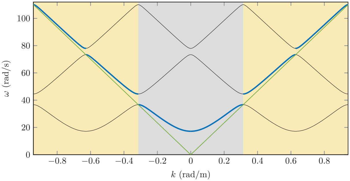
Dispersion curves of the periodic system in three Brillouin zones (black and blue lines) and the dispersion curve of the unsupported string (green line); the different Brillouin zones are indicated through different background colour. The primary dispersion curve is displayed with the thick blue lines while the secondary ones with thin black lines.

Returning to the problem with the moving load, we still need to impose two boundary conditions to have a fully determined solution. Because we are searching for the steady-state response, we can make use of the so-called periodicity condition [10]. For the considered system (the load does not have an inherent frequency), the response inside each cell is exactly the same as in the previous one but shifted in time by $d / v$ . The two boundary conditions, therefore, read

\begin{matrix} {\tilde{w}}_{1} (x = nd) e^{- i ω \frac{d}{v}} = {\tilde{w}}_{2} (x = (n + 1) d), \\ \tilde{w}'_{1} (x = nd) e^{- i ω \frac{d}{v}} = \tilde{w}'_{2} (x = (n + 1) d) . \end{matrix}

(13)

Using equation (13), we can determine the remaining two unknown amplitudes $C_{1}$ and $C_{2}$ (their expressions can be found in Vesnitskii and Metrikin [10]). The steady-state solution in the Fourier domain is now determined. To obtain the time-domain solution, the inverse Fourier transform is performed numerically (for which to work efficiently, a small amount of damping is introduced.)

For a continuously supported string, the steady-state response does not exhibit any wave propagation away from the load (we only consider sub-critical velocities). For the discretely supported string, however, waves are excited from the load every time it passes a support. In the case of a single support, the load generates a continuous wave spectrum when it passes it; this phenomenon is called transition radiation [25 –30]. In the periodic system, the waves generated at each support interfere (constructively for some frequencies and destructively for others) leading to a discrete frequency spectrum of the radiated waves; this phenomenon is sometimes called resonance transition radiation [26] because the constructive interference of the radiated waves leads to resonance for some system parameters. More specifically, resonance occurs when the group velocity of one generated wave is equal to the load velocity. From Figure 10, we can identify the velocities at which resonance occurs (consider only the black line). As it can be seen, the system has many velocities at which resonance occurs, but some velocities lead to stronger resonance than others. Strong resonance occurs at low frequencies of the generated harmonic and at high velocities of the load [10].

To determine the frequency/wavenumbers of the waves generated by the moving load, next to the dispersion curve, we need another equation that expresses a relation between the frequency, wavenumber, and the load velocity, namely the kinematic invariant. For this system, the kinematic invariant can be determined from the following equation (10) ( a mathematical derivation of the kinematic invariants is given in Appendix 1):

\cos (kd) = \cos (\frac{ω d}{v}) .

(14)

Equation (14) shows that there are infinitely many kinematic invariants. The zeroth-order kinematic invariant is given by $ω = kv$ that relates to a constant moving load while the higher order kinematic invariants are given by $ω = kv + m \frac{2 π v}{d}$ with $m = \pm 1, \pm 2, \dots$ , and are related to moving harmonic loads of frequency $m \frac{2 π v}{d}$ .

Figure 3 presents the dispersion curve together with the kinematic invariants of the current problem. The dispersion curve is slightly different compared to the one in Figure 2 due to the presence of damping. It can be seen that there is no intersection point between the zeroth-order kinematic invariant (thick blue line) and primary dispersion curve (thick black line) because the considered load velocity is sub-critical; nonetheless, there are intersection points between higher-order components. The intersections between one of the kinematic invariants and the dispersion curve represent propagating waves emitted by the moving load in the steady state. Moreover, it is important to observe in Figure 3 that the emitted waves form a discrete frequency spectrum, as expected, and that all generated waves have frequencies in the pass bands of the system.

Figure 3.

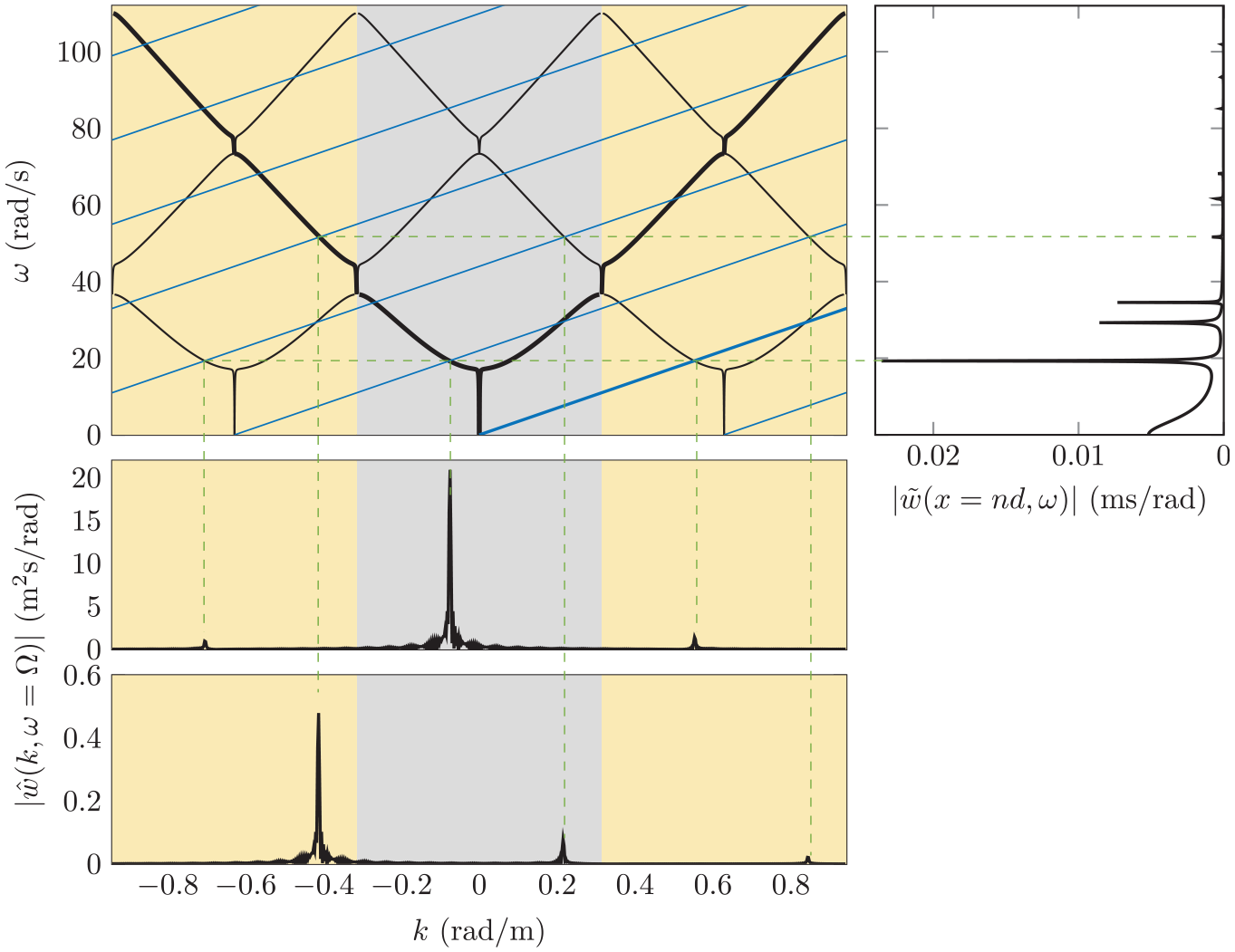
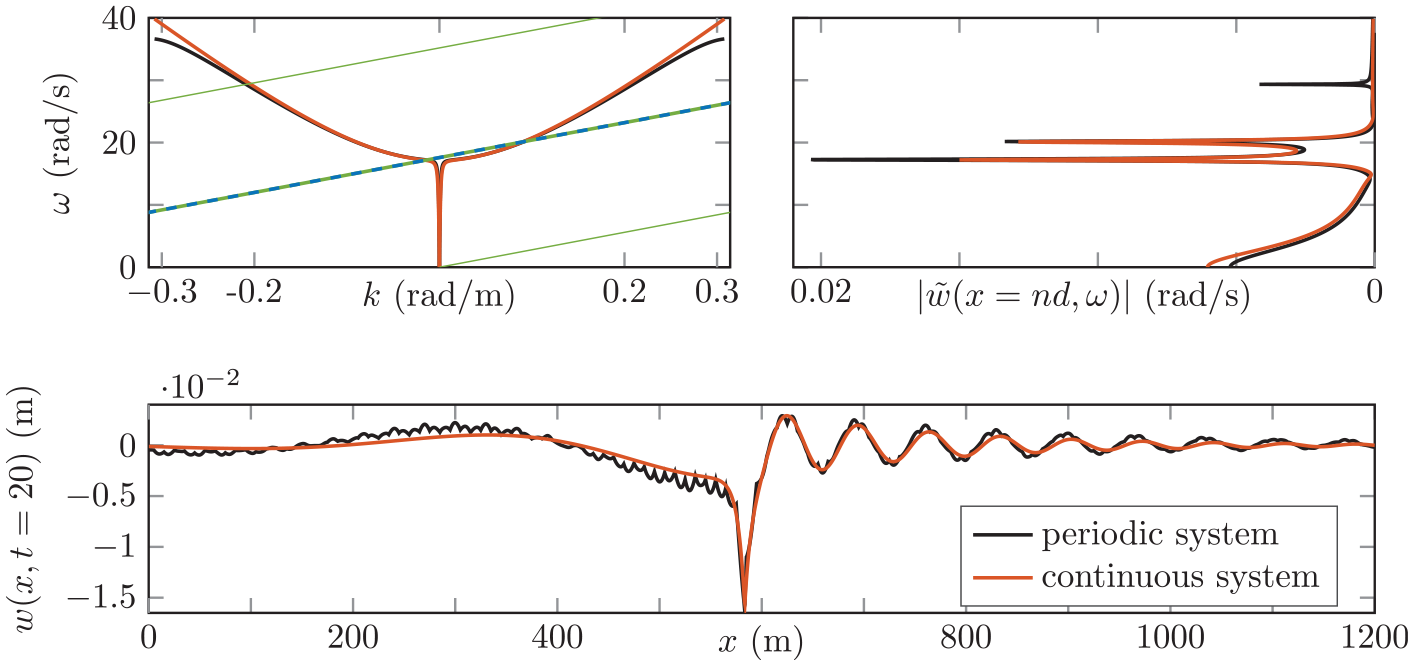
The dispersion curve (black solid lines) and the kinematic invariants (blue solid lines) (top left panel; $v \approx 0.25 c$ ), the frequency spectrum of the steady-state displacement (top right panel), and the wavenumber spectra of the steady-state displacement (bottom panels) evaluated at $Ω = 19$ and $Ω = 51$ rad/s (indicated by the horizontal dashed lines).

Moreover, it is clear from the wavenumber spectrum that the wave pack with frequency $ω$ (e.g. $ω = 19$ or $ω = 51$ rad/s depicted in Figure 3 through the dashed green lines) is composed of infinitely many discrete harmonic waves. The reason is that the harmonic wave is not an eigen-solution of the equation of motion; consequently, the eigenfunction is represented as a superposition of infinitely many harmonic waves. Some of these harmonic waves have a negative phase velocity while others have a positive one. Nonetheless, the wave pack ( $ω = 19$ or $ω = 51$ rad/s) has a negative group velocity meaning that it travels in negative $x$ direction. Also, the main contribution to the wave pack can be seen to come from the intersection of one of the kinematic invariants with the primary dispersion curve, as explained previously.

Figure 4 presents a time-domain snapshot of the steady-state displacement field. It can be observed that in front of the load, the wave is mainly governed by one frequency-wavenumber pair while behind more pairs seem to be influential; also, the amplitude of the wave behind the load is larger than the one in front. The wave in front of the load is mainly governed by the second peak in the frequency spectrum which is associated with a positive group velocity larger than the load speed (so it travels in front of the load; see top plots in Figure 3) while the one behind the load is governed by the first and third peaks which are associated with negative group velocities; this explains the difference in amplitude as well as the frequency-wavenumber content of the waves.

Figure 4.

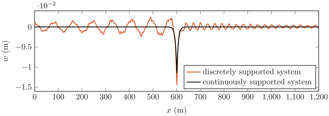
Snapshot of the time-domain displacement field for the discretely and continuously supported systems.

4. Inhomogeneous system

In this section, the periodic system with a transition zone (as depicted in Figure 1) is considered. The solution is obtained using a Green’s function approach; the moving load is first assumed to act inside only one cell and the response of this system is determined. To obtain the response of the system to the moving load acting on all cells, the individual solutions are superimposed. The drawback of this approach is that the load cannot act from $t \to - \infty$ since this would imply obtaining and adding infinitely many solutions. Nonetheless, if the load enters far away to the left of the transition zone and if the system has damping, the response in the transition zone should be in the steady state. (This shortcoming could be avoided by imposing the steady state as initial conditions of the system (see Fărăgău et al. [29]); this is not done here because the computational cost of the above-mentioned procedure is very low.)

The solution procedure starts, as previously, by applying the Fourier transform over time to equation (1). Then, the loading obtained is only considered for one cell; the solution procedure is demonstrated for the situation in which the load is applied to the left of the stiff zone, but the same procedure needs to be followed when it acts inside the stiff zone or to the right of it. The obtained equation of motion is divided in 5 domains: (1) left of the loaded cell, (2) the loaded cell, (3) right of the loaded cell and left of the stiff zone, (4) inside the stiff zone, and (5) to the right of the stiff zone. Their solutions can be written as done in the previous section and read

{\tilde{w}}_{1, n, n_{ξ}} = a_{2} e^{- i k_{2}^{F} nd} u_{2}, n < n_{ξ},

(15)

{\tilde{w}}_{2, n, n_{ξ}} = b_{1} e^{- i k_{1}^{F} nd} u_{1} + b_{2} e^{- i k_{2}^{F} nd} u_{2} + {\tilde{w}}_{n}^{ML}, n = n_{ξ}

(16)

{\tilde{w}}_{3, n, n_{ξ}} = c_{1} e^{- i k_{1}^{F} nd} u_{1} + c_{2} e^{- i k_{2}^{F} nd} u_{2}, n_{ξ} < n < n_{a},

(17)

{\tilde{w}}_{4, n, n_{ξ}} = d_{1} e^{- i {\bar{k}}_{1}^{F} nd} {\bar{u}}_{1} + d_{2} e^{- i {\bar{k}}_{2}^{F} nd} {\bar{u}}_{2}, n_{a} \leq n < n_{b},

(18)

{\tilde{w}}_{5, n, n_{ξ}} = e_{1} e^{- i k_{1}^{F} nd} u_{1}, n \geq n_{b} .

(19)

where $n$ is the left interface of the observation cell, $n_{ξ}$ is the left interface of the loaded cell (i.e. the excitation cell), and the overbar indicates that the quantity is associated to the stiff zone; $n_{a}$ and $n_{b} - 1$ are the left interfaces of the first and last cells, respectively, in the stiff zone. The boundary conditions at infinity have already been accounted for in these solutions. Also, the signs of the wavenumbers have been chosen as Im $(k_{1}^{F}) < 0$ and Im $(k_{2}^{F}) > 0$ . To determine the unknown amplitudes, interface conditions are imposed between the domains in the form of continuity in displacements and forces. The total solution (for the moving load acting on all considered cells) becomes

{\tilde{w}}_{n} = \sum_{n_{ξ} = N_{left}}^{N_{right}} {\tilde{w}}_{n, n_{ξ}},

(20)

where ${\tilde{w}}_{n, n_{ξ}} = [{\tilde{w}}_{1, n, n_{ξ}}, {\tilde{w}}_{2, n, n_{ξ}}, {\tilde{w}}_{3, n, n_{ξ}}, {\tilde{w}}_{4, n, n_{ξ}}, {\tilde{w}}_{5, n, n_{ξ}}]$ is the solution for all the cells when the load is applied at $n_{ξ}$ , $N_{left}$ is the first cell on which the load acts (at $t = 0$ ) and $N_{right}$ represents the last cell. $N_{left}$ needs to be chosen sufficiently to the left of the transition zone such that the response is in the steady state in the transition zone. $N_{right}$ can be chosen based on the maximum time of the simulation and it does not introduce any unwanted transients in the response. It must be mentioned that the domain for which the response is determined can be and, for computational efficiency, should be smaller than the domain over which the load is applied. In other words, if $N_{left}$ is chosen far to the left of the transition zone, there is no need to determine the response there; we can restrict our domain of interest (i.e. observation) in the transition zone.

The solution is now determined at the interfaces between cells. To determine the solution inside the cells, one simply needs to use equation (8). In the following, three phenomena are described and investigated that occur due to the combination of periodicity with the local inhomogeneity and lead to response amplification.

4.1. Wave-interference phenomenon

Figure 3 shows that, in the case of a homogeneous system, the frequencies of all emitted waves lie inside the pass bands. However, once there is a change in stiffness of the supporting structure (i.e. a transition zone), the locations of the stop bands are different for the different parts of the infinite domain. Consequently, the frequencies of waves excited by the load in the soft regions can be in the stop band of the stiff zone. This causes the waves to be reflected almost completely by the stiff zone and to interfere with the wave field travelling with the load. This wave interference can lead to amplifications of the response in the transition zone.

For this mechanism to be pronounced, the amplitude of the waves that are in the stop band of the stiff zone should be significant. This criterion is met when the velocity is close to a resonance velocity. In Figure 10, the strongest resonance in the soft region occurs at a velocity $v \approx 26$ m/s; consequently, for this investigation, a velocity slightly higher than this one is chosen (i.e. $v = 28$ m/s). This is done because the excited wave needs to propagate faster than the load such that it has time to reflect from the stiff region. (At resonance, the group velocity of the generated wave equals the load velocity; for a load velocity slightly larger than resonance velocity, the generated wave of interest travels slightly faster than the load.)

There are two situations which lead to amplification of the response in the transition zone. First, the forward propagating wave is reflected at the stiff region and propagates backwards interfering with the wave field close to the load. This amplification should be observable at the left of the stiff region. Second, when the load has passed the stiff region, the backward propagating wave is reflected at the stiff zone and propagates forward interfering with wave field close to load. This amplification should be observable to the right of the stiff zone.

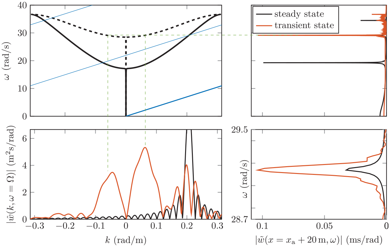
First, we investigate the region to the left of the stiff zone. The response is evaluated at approximately 5 m to the left of $x_{a}$ (see Figure 1); the frequency and wavenumber spectra of the transient response are compared to the steady-state ones in Figure 5. On one hand, the second peak in the frequency spectrum, corresponding to the forward propagating wave, is amplified in the transient response; because the frequency of this wave is in the stop band of the stiff zone, the wave is reflected almost in its entirety (not completely due to damping and transmission to the right of the stiff region). Moreover, unlike the steady-state response, the wavenumber spectrum of the transient response exhibits an additional wave with wavenumber equal in magnitude but opposite in sign (i.e. opposite direction of propagation) to that of the forward propagating wave, confirming the wave reflection. On the other hand, we can see that the first peak in the frequency spectrum, corresponding to backward propagating wave, is almost completely eliminated; the fact that the response is evaluated very close to the stiff zone (to its left) implies that less time is available to generate this wave (in the stiff zone, this wave is no longer generated), which explains the lower amplitude.

Figure 5.

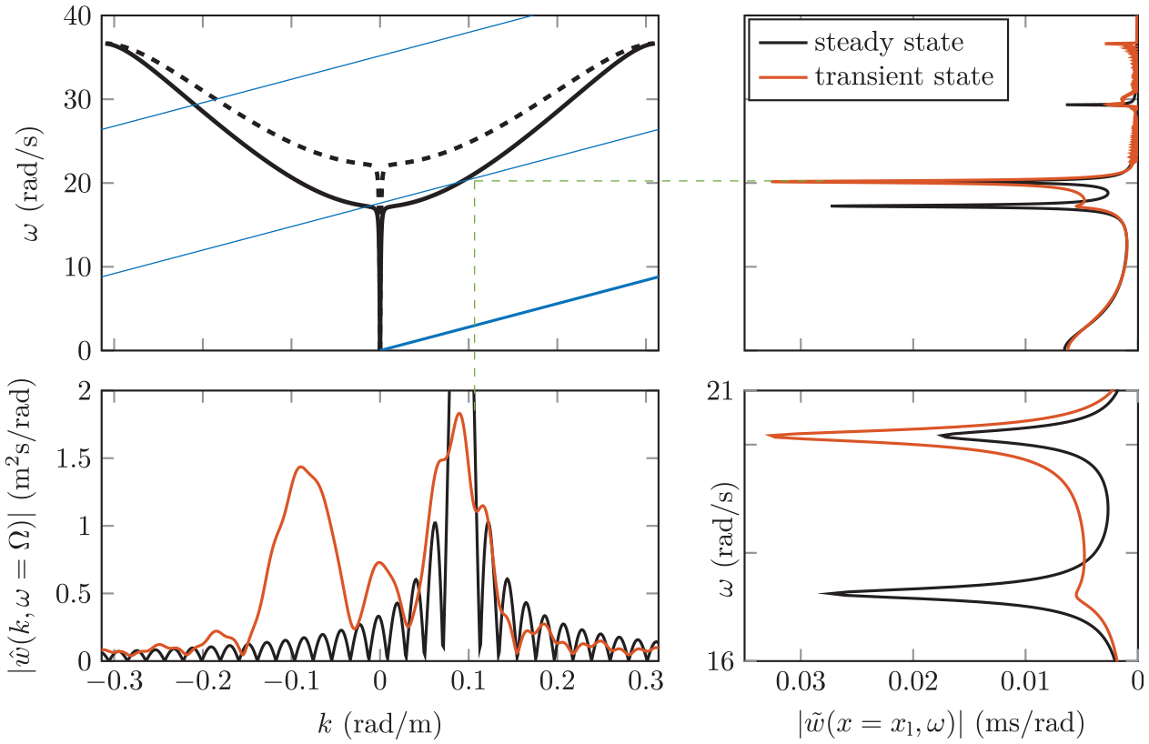
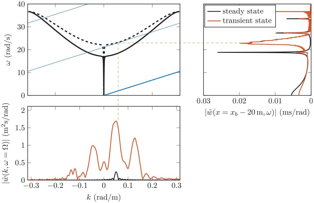
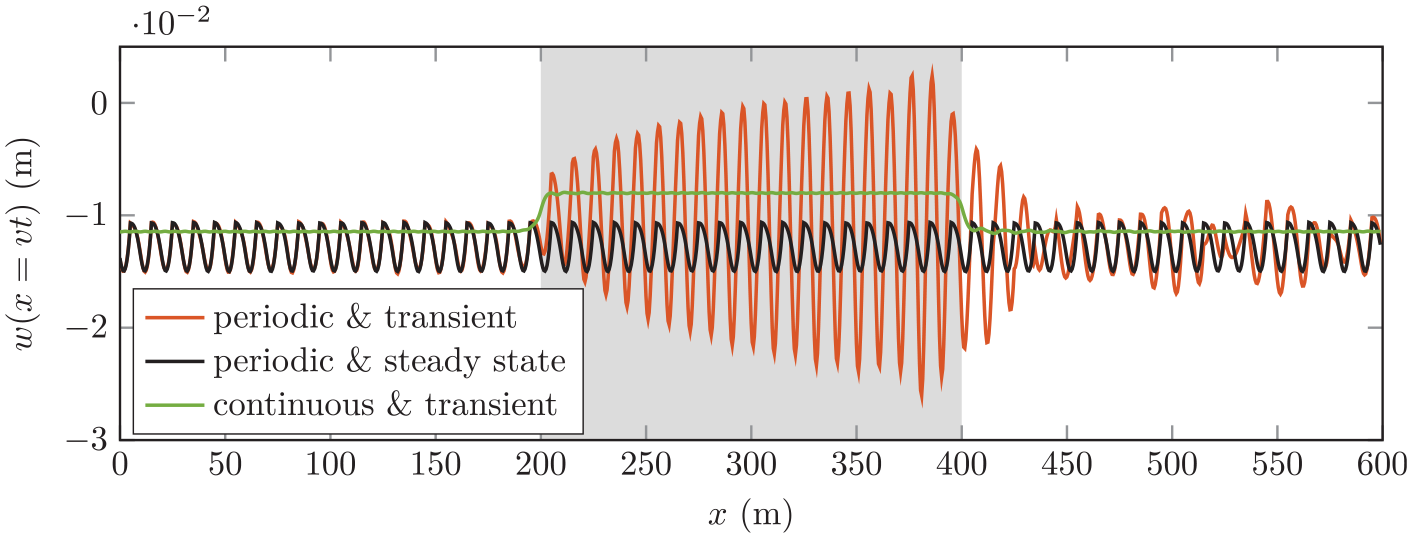
The primary dispersion curves for the soft (black solid line) and stiff (black dashed line) regions and the kinematic invariants (blue lines) (top left panel; $v = 28$ m/s), the frequency spectra of the displacements at a position $x_{l} = x_{a} - 5$ m to the left of and near the stiff zone (top right panel), and the wavenumber spectra of the displacements (bottom left panel) evaluated at $Ω = 20.2$ rad/s (indicated by the horizontal green dashed line); the bottom right panel is a zoom in of the top right panel.

When looking to the right of the stiff zone, the opposite is occurring. Figure 6 shows that the first peak in the frequency spectrum is amplified while the second peak is almost completely eliminated in the transient response. A similar reasoning as above can be used to explain these observations. A general picture is obtained when looking at the time-domain response under the moving load, presented in Figure 7. The transient response is amplified significantly to the left and right of the stiff region.

Figure 6.

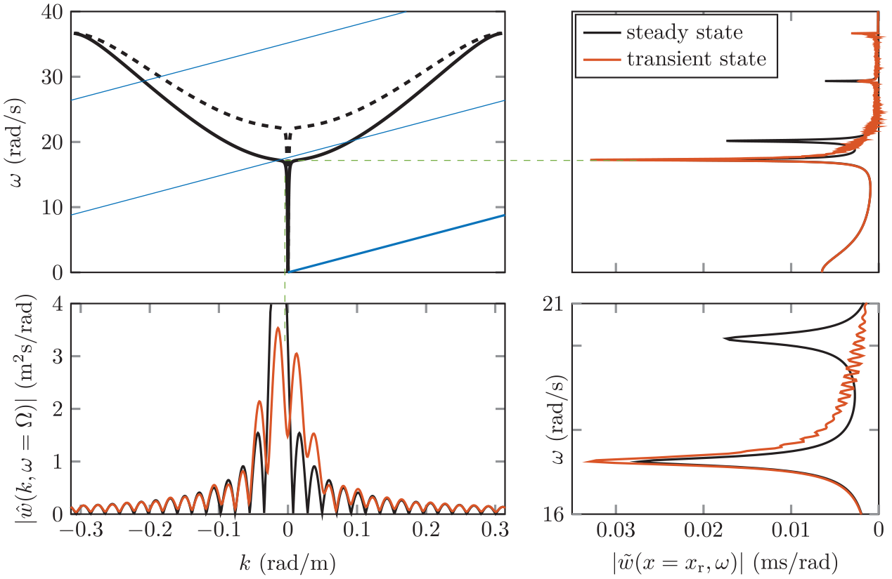
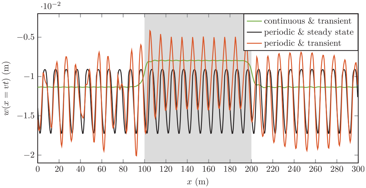
The primary dispersion curves for the soft (black solid line) and stiff (black dashed line) regions and the kinematic invariants (blue lines) (top left panel; $v = 28$ m/s), the frequency spectra of the displacements at position $x_{r} = x_{b} + 15$ m to the right of and near the stiff zone (top right panel), and the wavenumber spectra of displacements (bottom left panel) evaluated at $Ω = 17.2$ rad/s (indicated by the horizontal green dashed line); the bottom right panel is a zoom in of the top right panel.

Figure 7.

The displacement evaluated under the moving load for the wave-interference phenomenon; the location of the stiff zone is indicated by the grey background.

The response for the equivalent continuously supported system with a transition zone is also presented to show, that in that case, there is no visible amplification (due to the relatively low velocity). It is now clear that this significant amplification is caused by the periodicity of the system together with the transition zone; if any of these two characteristics are removed, the amplification vanishes.

The question arises how this mechanism is affected by the length of the stiff zone. If the stiff zone has a very short length, the tunnelling effect (similar to the quantum tunnelling [31]) can occur leading to energy being tunnelled to the soft domain to the right of the stiff zone. As a short investigation, we consider the same system, but an incident wave coming from the left is used instead of the moving load. The solution to that problem (cf. equations (15)–(19)) reads

{\tilde{w}}_{1, n} = A_{i} e^{- i k_{1}^{F} (n - n_{a}) d} u_{1} + A_{r} e^{- i k_{2}^{F} (n - n_{a}) d} u_{2}, n < n_{a},

(21)

{\tilde{w}}_{2, n} = A_{1} e^{- i {\bar{k}}_{1}^{F} (n - n_{a}) d} {\bar{u}}_{1} + A_{2} e^{- i {\bar{k}}_{2}^{F} (n - n_{a}) d} {\bar{u}}_{2}, n_{a} \leq n < n_{b},

(22)

{\tilde{w}}_{3, n} = A_{t} e^{- i k_{1}^{F} (n - n_{b}) d} u_{1}, n \geq n_{b} .

(23)

where $A_{i}$ , $A_{r}$ , and $A_{t}$ are the amplitudes of the incident, reflected, and transmitted waves, respectively; $A_{1}$ and $A_{2}$ are the amplitudes of the waves inside the stiff zone. Equation (23) together with the continuity conditions at the interfaces of the three domains can be used to express the amplitudes of all waves in terms of the amplitude of the incident wave $A_{i}$ . This allows us to study the reflected and transmitted waves depending on the frequency/wavenumber of the incoming wave and on the length of the stiff zone.

Figure 8 presents the coefficients $| A_{r, t} |^{2}$ of the reflected and transmitted waves, respectively, for three lengths of the stiff zone, where the length of the stiff zone is defined as $l = rd$ (i.e. an integer number of cells). (The coefficients $| A_{r, t} |^{2}$ are presented and not the amplitudes themselves because $| A_{r} |^{2} + | A_{t} |^{2} = | A_{i} |^{2}$ in the absence of damping [31]). Both coefficients are very small for frequencies below the cut-off frequency of the soft zone; in this frequency range, the incoming wave is evanescent, leading to no energy input. For frequencies in the pass band of both domains, the coefficient of the transmitted wave is dominant while that of the reflected one is low. In the frequency range between the cut-off frequencies of the two domains, the outcome depends highly on the length of the stiff zone. For a large $r$ , the coefficient of the transmitted wave is zero while the reflected one is almost 1 (it is not exactly 1 due to the presence of damping). For a smaller $r$ , energy is tunnelled to the right side and the transmission increases while the reflection decreases. The energy tunnelling to the right domain can be observed in the top panel of Figure 9.

Figure 8.

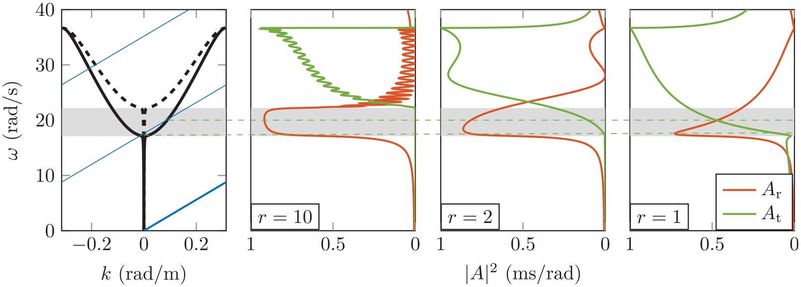
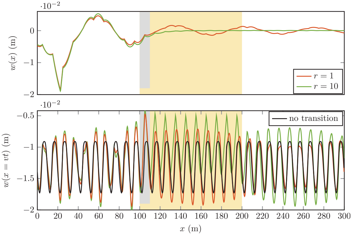
The primary dispersion curves for the soft (black solid line) and stiff (black dashed line) regions and the kinematic invariants (blue lines) (left panel; $v = 28$ m/s), and the coefficients of the reflected and transmitted waves (the three panels on the right) for three lengths of the stiff region; the frequency range between the cut-off frequencies of the two domains is indicated by the grey background.

Figure 9.

Snapshot of the displacement fields (top panel) and the displacements under the moving load (bottom panel) for a short stiff zone ( $r = 1$ ; the position of the stiff zone is indicated through the grey background) and a long one ( $r = 10$ ; the position of the stiff zone is indicated through the yellow background).

Returning to the problem with the moving load, the frequencies of the two dominant waves excited by the moving load (in the scenario studied previously; see Figure 5) are both in between the cut-off frequencies of the two domains. For a large $r$ , both waves experience almost full reflection, and thus, the significant amplification observed previously. For $r = 1$ , the forward propagating wave will not any more fully reflect, as can be inferred from the right panel of Figure 8 (the forward propagating wave is indicated through the top green dashed line), while the backward propagating wave is still almost fully reflected (the backward propagating wave is indicated through the bottom green dashed line). This scenario should lead to a smaller amplification to the left of the stiff zone and the same amplification to the right of the stiff zone. This is confirmed in the bottom panel of Figure 9, where the amplification to the left of the stiff zone is slightly smaller for $r = 1$ than for $r = 10$ , while the amplification to the right of the stiff zone is almost the same (there is a shift in time and space due to the different lengths of the stiff zone, so one needs to compare peaks at 115 m (orange) and 205 m (green)). Nonetheless, the amplification to the left of the stiff zone can be clearly seen even for $r = 1$ .

It is important to mention that the wave-interference phenomenon is not sensitive to the stiffness difference between the stiff and soft domain, provided that the generated waves are in the pass band of the stiff zone. Simulations have been performed also for $p = 5$ instead of $p = 2$ and the amplification turned out to be very similar in magnitude. Also, it must be mentioned that the wave-interference mechanism occurs also in the continuously supported system subject to a moving constant load, leading to amplification of the response as shown for a beam by Fărăgău et al. [28]; however, for a continuously supported system subject to a moving constant load, this mechanism is influential only for velocities close to the critical velocity while here it can lead to a significant response amplification for much lower velocities of the load.

4.2. Passing from non-resonance velocity to a resonance velocity

As discussed in Section 3, there are several load velocities that can lead to resonance in the periodic system. When designing the catenary system, its properties should be chosen such that these resonance velocities are far away from operational velocities of trains. However, even if the operational velocity is far from resonance velocities outside transition zones, it can be close to a resonance velocity inside the stiff region of the transition zone if this is not designed having this criterion in mind. In this section, the situation is investigated in which the load passes from non-resonance velocity in the soft region to a resonance velocity inside the stiff region. Note that the velocity of the load is kept constant and just the velocity at which resonance occurs changes due to a change of the support stiffness.

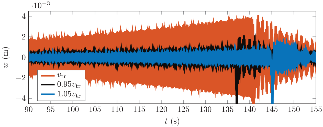
Figure 10 presents the resonance velocities for the soft and stiff regions (here the stiffness ratio is $p = 2$ ). For a load velocity of $v = 33.5$ m/s, the response is non-resonant in the soft region while in the stiff region it is expected to get amplified due to the occurrence of resonance. The fact that this velocity causes resonance in the stiff region can also be seen in the dispersion curve presented in Figure 11; one kinematic invariant (the first-order one) is tangential to the dispersion curve of the stiff region meaning that the group velocity of the generated wave is equal to the load velocity, which leads to resonance. The amplification of the response in the stiff zone can be observed in both the frequency spectrum and wavenumber spectrum. Moreover, the frequency and wavenumber spectra exhibit additional large peaks at the frequency and wavenumber, respectively, corresponding to the wave generated inside the stiff zone.

Figure 10.

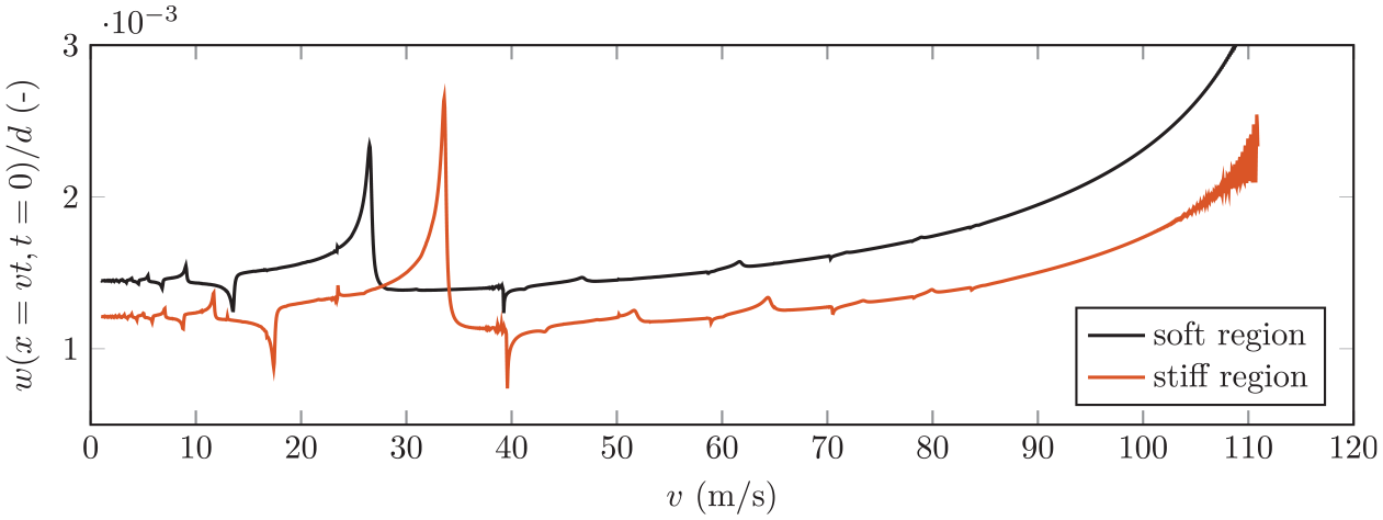
Load velocities that lead to resonance in the soft and stiff regions: normalized displacement under the moving load at $t = 0$ versus velocity.

Figure 11.

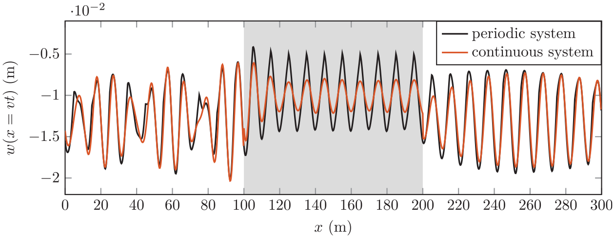
The primary dispersion curves for the soft (black solid line) and stiff (black dashed line) regions and the kinematic invariants (blue lines) (top left panel; $v = 33.5$ m/s), the frequency spectra of the displacements at a position inside the stiff zone (top right panel), and the wavenumber spectra of displacements (bottom left panel) evaluated at $Ω = 23$ rad/s (indicated by the horizontal green dashed line).

Figure 12 presents the displacement under the moving load. The amplification in the stiff zone is observed clearly with a drastic increase compared to the response in the soft region. The increase in response requires a few cell lengths to develop, characteristic to resonance; for short stiff zones, resonance might not have time to develop, but for longer ones, strong response amplification can develop.

Figure 12.

The displacements evaluated under the moving load for the resonance velocity in the stiff zone; the location of the stiff zone is indicated by the grey background.

It is important to mention that the phenomenon of passing to resonance velocity has an equivalent in the continuously supported system subject to a moving constant load, but there are important distinctions. First, in the continuous system, resonance can only occur at the critical velocity (the boundary between sub-critical and super-critical velocities) that usually is much larger than the operational train velocities. For example, the continuous system equivalent to the periodic one considered in this section has a critical velocity of around 115 m/s while the velocity that leads to the considered resonance in the stiff region is 33.5 m/s. Second, to go from sub-critical to critical velocity, the stiffness of the supporting structure needs to decrease (if all other parameters are kept constant); this is much less common in practice because transition zones are usually regions with stiffer structures.

4.3. Wave trapping inside the stiff zone

The stiff zone has a finite length $l$ , and consequently, the incoming waves generated by the moving load in the soft region could get trapped inside. Wave trapping could lead to response amplification inside the stiff zone even when the moving load is relatively far away. To mathematically derive the conditions for wave trapping, a system without damping is used, while in the graphical results a small amount of damping is present; however, the change in the wave-trapping conditions caused by a small amount of damping is negligible. The amount of damping imposed in this subsection is one quarter of that used in the rest of the paper to be able to present this mechanism in its purest form; for larger amounts of damping, although the mechanism can still be seen, it is less pronounced.

An approximate condition for wave trapping is that $q$ half-wavelengths of the wave inside the stiff zone is an integer fraction of $l$ . Mathematically this can be written as

q \frac{1}{2} λ = l = rd, q \in N, r \in N,

(24)

where $λ$ is the wavelength. This would only be exact if the stiff zone was simply supported at both ends, which is not the case for the considered system. An exact condition for the considered system can be derived by using the phase-closure principle (see Mead [32]) to determine the modes of vibration of the stiff zone. However, this exceeds the purpose of the paper and the approximate condition is sufficient to observe the mechanism.

From relation (24) the wavenumber $k_{tr}$ for the wave to be trapped is determined and it reads

k_{tr} = \frac{q π}{rd} .

(25)

In order to find the corresponding frequency, the wavenumber in the first Brillouin zone is chosen because the waves with most energy generated by the moving load are located in the first pass band (the higher harmonics have significantly less energy) and the first Brillouin zone. The frequency $ω_{tr}$ corresponding to $k_{tr}$ can be found by numerically solving the dispersion equation for $ω_{tr}$

\cos (\frac{q π}{r}) = \frac{(p k_{s}) c}{2 T ω_{tr}} \sin (\frac{ω_{tr} d}{c}) + \cos (\frac{ω_{tr} d}{c}) .

(26)

A wave with wavenumber $k_{tr}$ given by Eq. (25) and frequency $ω_{tr}$ would be trapped inside the stiff zone. The wavenumber $k_{tr, 2}$ of the generated wave in the soft region (the frequency remains the same $ω_{tr}$ ) reads

k_{tr, 2} = \frac{1}{d} \arccos (\frac{1}{p} \cos (\frac{q π}{r}) + \frac{p - 1}{p} \cos (\frac{ω_{tr} d}{c})) .

(27)

Clearly, the wave with wavenumber $k_{tr, 2}$ and frequency $ω_{tr}$ generated in the soft region will give rise to a wave in the stiff region that is trapped. One can easily check this by considering the system with a harmonic load (acting at a location in the open track) instead of a moving one, in which case the wave trapping can be clearly observed (this result is not presented here for conciseness). To observe the same behaviour for the moving load, one first needs to determine the velocity of the load at which this wave (wavenumber $k_{tr, 2}$ and frequency $ω_{tr}$ ) is generated. To this end, we substitute $k = k_{tr, 2}$ and $ω = ω_{tr}$ in the kinematic invariant, equation (14). Because sub-critical velocities are considered, the zeroth-order kinematic invariant cannot intersect the primary dispersion curve; therefore, we look at the first-order kinematic invariant, and the velocity of the load corresponding to this situation reads

v_{tr} = \frac{ω_{tr} d}{k_{tr, 2} d + 2 π} .

(28)

The frequency and wavenumber spectra evaluated at a position inside the stiff zone are presented in Figure 13. The frequency spectrum of the transient response exhibits a large peak at $ω_{tr}$ corresponding to the trapped wave. Moreover, the wavenumber spectrum shows that the wave in the soft region with wavenumber $k_{tr, 2}$ (represented by the black line) is transformed in the stiff region into two peaks at $k_{tr}$ and $- k_{tr}$ that represent the trapped (standing) wave inside the stiff zone. The two peaks are not equal in magnitude as would be the case for a true standing wave. One reason is that, as the source is on the left of the stiff region, the wave travelling in negative $x$ direction (which is a reflection of the wave travelling in positive $x$ direction) is damped more; another reason is that energy is transmitted to the right of the stiff domain. Figure 14 presents a snapshot of the displacement field where the trapped wave can be clearly observed. The amplification is not drastic, but it is clear. In Figure 14 can also be seen that energy is transmitted to the right domain, meaning that even in the absence of damping, the amplification in the stiff domain will not be infinite. Moreover, it is important to realize that only the wave corresponding to the second peak (in the frequency domain) is trapped; all other waves can pass through. Finally, the amplification disappears for slightly different velocities, as can be seen in Figure 15, or different lengths of the stiff zone (provided that it is not another multiple of the wavelength).

Figure 13.

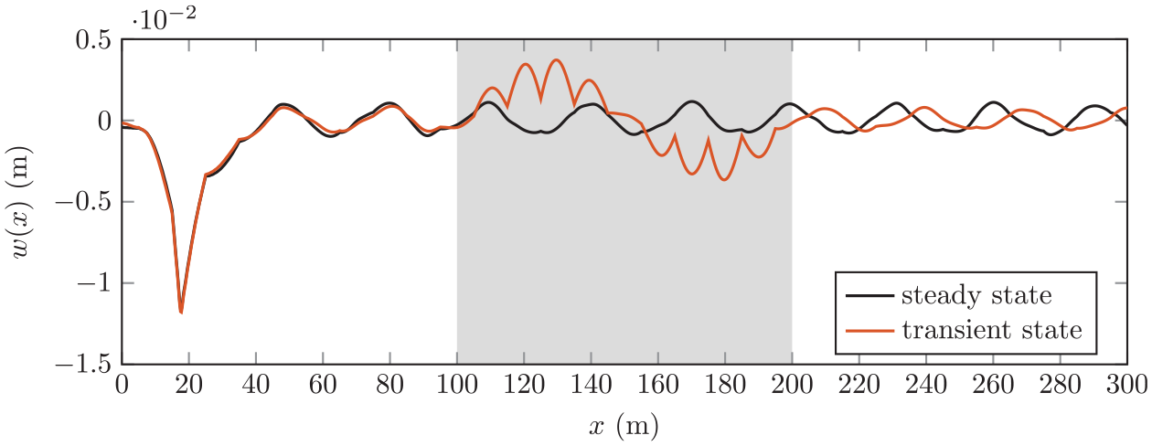
The primary dispersion curves for the soft (black solid line) and stiff (black dashed line) regions and the kinematic invariants (blue lines) (top left panel; $v = 34.5$ m/s), the frequency spectra of the displacements at a position inside the stiff zone (top right panel), and the wavenumber spectra of displacements (bottom left panel) evaluated at $Ω = 28.6$ rad/s (indicated by the horizontal green dashed line); the bottom right panel is a zoom in of the top right panel.

Figure 14.

Snapshot of the time-domain displacements for the situation when the wave is trapped in the stiff zone; the stiff zone is indicated by the grey background.

Figure 15.

Displacement time history evaluated inside the stiff zone for slightly different load velocities.

5. Relation to the continuously supported system with a harmonic moving load

An easier problem to solve that could also capture the three phenomena discussed in Section 4 is the continuously supported string subject to a moving harmonic load. The solution of this problem can be obtained by applying the Fourier transform over time to the governing equations and solving the resulting ordinary differential equation in the Fourier-space domain. This has been done in, for example [28,33], for a moving constant load and can easily be extended to a moving harmonic load.

The frequency of the harmonic load can be chosen such that the first two peaks in the frequency spectrum (e.g. Figure 3) are accurately represented; by choosing $Ω = \frac{2 π v}{d}$ , the kinematic invariant in the continuously supported system coincides with the first-order kinematic invariant from the periodic system. Moreover, for the responses of the two systems to match, the moving load must have two components: a constant one (zero frequency) and a harmonic one; this way, the response is not symmetric with respect to the zero displacement line, but is shifted downwards as seen in Figure 7. Thus, the expression for the moving harmonic load reads $- F_{0} (p_{1} + p_{2} \cos (Ω t)) δ (x - vt)$ , where $p_{1}$ and $p_{2}$ need to be tuned such that the overall steady-state displacement field matches the one of the periodic system.

Figure 16 presents the comparison of the periodic and continuous systems. It can be seen that the frequency spectra of the two systems agree well for the first two peaks, and the continuous system does not exhibit more peaks than these two. One can introduce more peaks in the response of the continuous system by imposing multiple harmonic components to the moving load (i.e. $p_{3} \cos (2 Ω t)$ , etc.). The bottom panel in Figure 16 shows that the time-domain displacement fields also agree well. For this set of parameters, $p_{1} = 1$ and $p_{2} = 0.1$ lead to the best fit overall; it must be emphasized that these tuning parameters change with system properties (e.g. load velocity, support spacing, support stiffness, etc.), and they cannot be determined without the response of the periodic system.

Figure 16.

Comparison of the periodic system and continuous one; the dispersion curves and the kinematic invariants (top left panel), the frequency spectra of the steady-state displacements (top right panel), and a snapshot of the time-domain displacements (bottom panel).

First, when it comes to the wave-interference mechanism, Figure 17 shows that the transient response of the continuous system exhibits qualitatively the same behaviour as the periodic one. However, the response in the stiff region differs considerably between the two systems because parameters $p_{1}$ and $p_{2}$ have been chosen such that the responses match in the soft region, not in the stiff one. This is one drawback of the equivalent model if one is interested in the response inside the stiff region. Also, the wave-interference mechanism can be reproduced in the continuous system only if the waves (in the periodic system) with most energy are located in the first stop band of the stiff region; if these waves were in the second stop band, then they would be able to propagate through the stiff zone of the continuous system because, unlike the periodic one, it only has one stop band. When it comes to the tunnelling effect, this can also occur in the continuously supported system and will lead to a decrease in the response amplification caused by the wave-interference phenomenon.

Figure 17.

Displacements evaluated under the moving load; the position of the stiff region is indicated by the grey background.

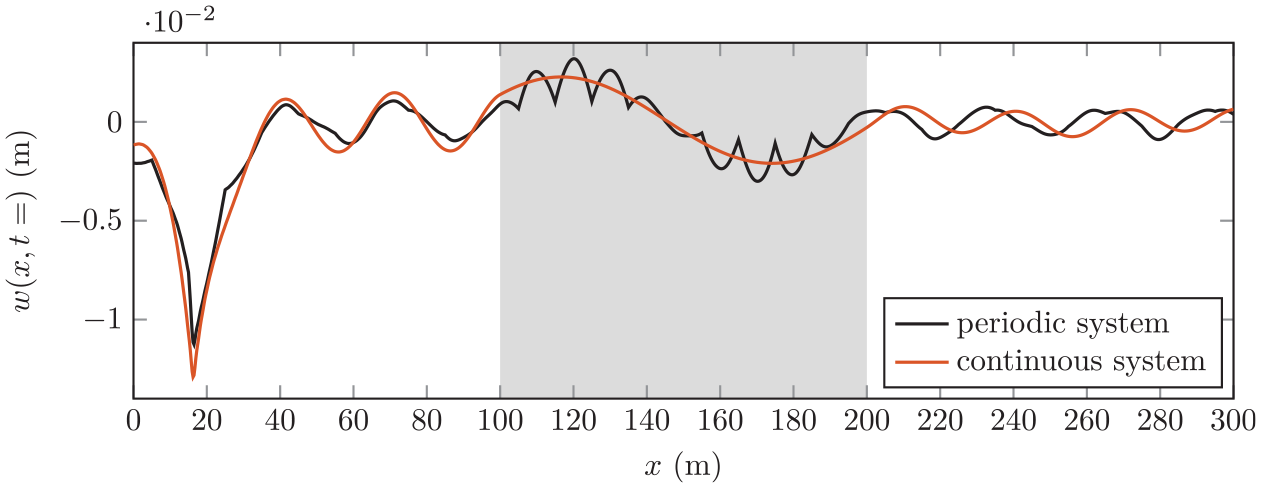
Second, for the wave-trapping phenomenon, Figure 18 shows that the continuous system exhibits a similar behaviour as the periodic one, and the agreement between the two is very good. If one wants to investigate this mechanism in detail, the continuous system can be an option. The fit between the transient responses can be further improved by changing the scaling factors $p_{1}$ and $p_{2}$ , but this would require to have the transient response of the periodic system in advance, defeating the purpose of using the continuous system.

Figure 18.

Snapshot of the time-domain displacements for the situation when the wave is trapped in the transition zone; the position of the stiff region is indicated by the grey background.

Finally, for passing from non-resonance velocity to resonance velocity, the continuous system cannot be used at all. The continuous system has one resonance velocity, the critical velocity; the value of that critical velocity is much higher than the one leading to resonance in Section 4.2. Consequently, this phenomenon can only be investigated in the periodic system.

6. Conclusion

This paper investigated three phenomena that can lead to response amplification in a continuous and periodic system with a local inhomogeneity (i.e. a transition zone) described by an increase in support stiffness. These phenomena are investigated using an infinite string periodically supported by discrete springs and dashpots, acted upon by a moving constant load; this model is representative of a catenary system in railway tracks. Nonetheless, the phenomena described in this paper can occur also in other continuous and periodic systems, such as a beam and membrane. The phenomena are the product of a periodic system and a local inhomogeneity, and if one of these characteristics is omitted, the phenomena will not occur.

The first phenomenon is the wave interference that can lead to response amplification to the left and to the right of the stiff region. The waves generated by the moving load outside the transition zone are reflected almost entirely by the stiff region if one of the frequencies of the waves are located in a stop band of the stiff region. This almost complete reflection leads to wave interference close to the moving load, which in turn leads to response amplification. Results show that this mechanism is of importance when the velocity of the load is slightly higher than one of the resonance velocities in the soft regions. For small lengths of the stiff zone energy can be tunnelled to the soft domain causing a reduction in the reflection coefficient which in turn leads to a reduced amplification.

The second phenomenon is the passing from non-resonance velocity in the soft region to a resonance velocity in the stiff region. This causes resonance to occur inside the stiff region leading to a drastic amplification of the response mainly inside the stiff region. Results show that this mechanism leads to the biggest response amplification between the three phenomena.

The third phenomenon is the wave trapping inside the stiff region. For specific values of the wavenumber and frequency of the waves generated in the soft region, waves can get trapped inside the stiff zone potentially leading to response amplification around and inside the stiff zone. Results show that this mechanism leads to amplification inside the stiff region even when the moving load is relatively far away from it. However, for reasonable values of damping, this mechanism is not as pronounced as the other two.

The possibility of capturing these phenomena using a simpler model, a continuously supported string acted upon by a moving harmonic load, was also studied. The wave-interference and wave-trapping phenomena observed in the periodic system can be seen in the continuous system too, while the resonance phenomenon cannot be replicated using the continuous model. To obtain similar results for the continuous system, the static and harmonic components need to be tuned to the steady-state response of the periodic system. Once this tuning is satisfactory, the transient responses match quite well and the two phenomena are qualitatively well captured. However, the tuning parameters, in principle, are not known before-hand and need to be updated for each change of the system properties, which makes it difficult to use the continuous system in practical situations.

Finally, the amplification of stresses and displacements in the transition zones can lead to numerous fatigue and wear problems in the catenary system and in the energy collector of the train. Moreover, accounting for the low (mean) contact force between wires and carbon strip, the dynamic response of the system can also lead to force fluctuations that are large enough to cause arching (occurs when the contact force is too low) or loss of contact. The three investigated phenomena can be considered as additional constraints for the design parameters at transition zones such that amplifications are avoided, especially because all three phenomena occur in the range of operational train speeds.

Footnotes

Appendix 1

Here we present a detailed derivation of the dispersion equation (equation (12)) and of the kinematic invariant (equation (14)). For clarity of the derivations, a system without damping is considered.

First, the dispersion curve is derived. The eigenvalues $α_{1, 2}$ are obtained from an eigenvalue analysis of the Floquet matrix. The Floquet matrix is obtained by evaluating the right-hand side of equation (8) (excluding the particular solutions) at $x = (n + 1) d$ , and reads

(29)

F = (\begin{matrix} \frac{k_{s} \sin (γ d)}{2 T γ} + \cos (γ d) & \frac{\sin (γ d)}{γ} - \frac{\cos (γ d) k_{s}}{2 T γ^{2}} + \frac{k_{s}}{2 T γ^{2}} \\ - \sin (γ d) γ + \frac{\cos (γ d) k_{s}}{2 T} + \frac{k_{s}}{2 T} & \frac{k_{s} \sin (γ d)}{2 T γ} + \cos (γ d) \end{matrix}) .

The determinant of the Floquet matrix is 1, and, thus, the eigenvalues of the Floquet matrix read

(30)

α_{1, 2} = B \pm \sqrt{B^{2} - 1}, B = \frac{k_{s} \sin (γ d)}{2 T γ} + \cos (γ d),

where $B$ is half the trace of $F$ . The relation between the Floquet wavenumber $k^{F}$ and the eigenvalue $α$ (we restrict the following derivation to one eigenvalue; the derivation is analogous for the other one) is given as follows:

(31)

α = e^{i k^{F} d} .

Depending on the frequency ( $B$ is frequency dependent), there are three possible scenarios. The first scenario is that $B^{2} > 1$ meaning that $α$ is real-valued and positive. From equation (31), this leads to the wavenumber $k^{F}$ to be purely imaginary; the corresponding frequency ranges represent the stop-bands in the dispersion curve. The second scenario is when $B^{2} = 1$ resulting in repeated eigenvalues. These locations correspond to the transition points between the stop and pass bands. For the third scenario, $B^{2} < 1$ resulting in complex-valued eigenvalue $α$ corresponding to the pass-bands in the dispersion curve; in this scenario, waves are propagating without attenuation meaning that $k^{F}$ is real-valued. Consequently, equation (31) can be rewritten as

(32)

α = \cos (k^{F} d) + i \sin (k^{F} d) .

This leads to the following set of conditions for the Floquet wavenumber

(33)

{\begin{matrix} \cos (k^{F} d) = B, \\ \sin (k^{F} d) = \sqrt{B^{2} - 1} \end{matrix} .

If the first condition in equation (33) is satisfied, then the second one is also satisfied. Any of the two conditions can be selected as the dispersion equation (we selected the first one due to its concise form).

Second, the kinematic invariants are derived. The kinematic invariants ensure phase equality of the emitted harmonic waves and the load at the contact point [10]. The phase of a harmonic wave with frequency $ω$ and wavenumber $k$ is

(34)

ϕ = ω t - kx .

The phase of a harmonic wave is constant for an observer moving together with the wave, resulting in the following relation between frequency and wavenumber:

(35)

ω = k \frac{d x}{d t} .

The change of position with time (i.e. $d x / d t$ ) of the moving load is its velocity $v$ , and since the kinematic invariant ensures phase equality of the emitted harmonic waves and the load, we have

(36)

ω = kv .

This is the kinematic invariant for a homogeneous system (without periodic supports) subject to a moving constant load. For the system studied in this paper (continuous system with discrete and periodic supports), a harmonic wave (with phase given by equation (34)) is not a solution of the equation of motion; the equation of motion allows for solutions in the shape of summations of harmonic waves that have the following expression for the phase:

(37)

ϕ = ω t - (k + m \frac{2 π}{d}) x,

where $m = \pm 1, \pm 2, \dots$ . In this case, infinitely many kinematic invariants are necessary to ensure phase equality between the moving load and the infinitely many generated waves. The expression of the kinematic invariants reads

(38)

ω = kv + m \frac{2 π v}{d} .

This expression is analogous to equation (14).

Appendix 2

Here we show why the branch of the dispersion curve of the periodic system closest to the dispersion curve of the unsupported string leads to more energetic waves than the other branches. One might think that all information is just repeated from one Brillouin zone to the next (like for discrete periodic systems), but that is not completely correct for a continuous system. Let us consider a wave field propagating in positive $x$ direction (i.e. the second term in equation (11) is zero). The normalized state at interface $nd$ would then read

(39)

\frac{w_{n}}{a_{1}} = e^{- i k_{1}^{F} nd} u_{1} .

The displacement inside the generic cell can be calculated using equation (8) without the particular solution, as follows:

(40)

\frac{\tilde{w} (x, ω)}{a_{1}} = (u_{1, 1} f_{1, 1} (x - nd) + u_{1, 2} f_{1, 2} (x - nd)) e^{- i k_{1}^{F} nd}, nd \leq x \leq (n + 1) d,

where $f_{1, 1} (x)$ and $f_{1, 2} (x)$ are the functions from equation (8). Furthermore, $u_{1, 1}$ and $u_{1, 2}$ represent the first and second entries in the eigenvector $u_{1}$ , respectively. To see which wavenumbers are present in $\tilde{w} (x, ω)$ , we can take the Fourier transform over space (note that $\bar{k} \in (- \infty, \infty)$ is the Fourier variable), and the scaled response $\hat{w} (\bar{k}, ω)$ in the frequency-wavenumber domain reads

(41)

\hat{w} (\bar{k}, ω) = \sum_{n = - \infty}^{\infty} \int_{nd}^{(n + 1) d} \frac{\tilde{w} (x, ω)}{a_{1}} e^{- i \bar{k} x} d x .

Provided that the sign of the imaginary part of $k_{1}^{F}$ is chosen properly (to represent a forward propagating wave), both the integral and the summation in equation (41) can be performed analytically. The result reads

(42)

\hat{w} (\bar{k}, ω) = A (γ, \bar{k}) \frac{1}{γ^{2} - {\bar{k}}^{2}} \frac{e^{i d (\bar{k} + k_{1, r}^{F})}}{e^{i d (\bar{k} + k_{1, r}^{F})} - e^{{dk}_{1, i}^{F}}},

where $k_{1, r}^{F}$ and $k_{1, i}^{F}$ are the real and imaginary parts of $k_{1}^{F}$ , respectively. Function $A (γ, \bar{k})$ contains terms proportional to $(\bar{k} \pm γ)$ ; these terms increase linearly with increasing $\bar{k}$ while the second factor in equation (42) is inversely proportional to ${\bar{k}}^{2}$ for large enough values of $\bar{k}$ ; this is the reason why the second factor was singled out while the other terms are contained in $A (γ, \bar{k})$ . The last factor in equation (42) gives the influence of the Floquet wavenumber (the periodic part of the system) on the response while the second factor gives the influence of the wavenumber of the unsupported string (the continuous part of the system); actually, the denominator of the second factor yields the dispersion curve of the unsupported string (when equated to zero). The last factor exhibits peaks of equal magnitude (infinite magnitude in the case of no damping) at $\bar{k} = - k_{1, r}^{F} \pm m \frac{2 π}{d}$ ; therefore, this factor associated with the Floquet wavenumbers does not make any distinction between Brillouin zones. The second factor, has a parabolic function in the denominator and decreases as $\bar{k}$ moves away from $γ$ . Therefore, the peaks of $\hat{w} (\bar{k}, ω)$ at $\bar{k} = - k_{1, r}^{F} \pm m \frac{2 π}{d}$ decrease in amplitude as $\bar{k}$ moves away from $γ$ . This is the mathematical reason why the branches closest to the dispersion curve of the unsupported string lead to most energetic waves. From a physical perspective, the energy propagated from cell to cell is governed by the Floquet wavenumbers; however, the propagation inside the cells is governed by the string, which imposes what branches of the dispersion curve lead to more or less energetic waves.

Funding

The author(s) disclosed receipt of the following financial support for the research, authorship, and/or publication of this article: This research is supported by the Dutch Technology Foundation TTW (Project 15968), part of the Netherlands Organization for Scientific Research (NWO), and which is partly funded by the Ministry of Economic Affairs.

ORCID iD

Andrei B. Fărăgău

References

Steenbergen

MJMM.

Physics of railroad degradation: the role of a varying dynamic stiffness and transition radiation processes. Comput Struct 2013; 124: 102–111.

Brillouin

Wave propagation in periodic structures. 2nd ed. Mineola, NY: Dover Publications, 1953.

Rayleigh

On the maintenance of vibrations by forces of double frequency, and on the propagation of waves through a medium endowed with a periodic structure. Philos Mag 1887; XXIV: 145–159.

Mead

DJ.

Free wave propagation in periodically supported, infinite beams. J Sound Vib 1970; 11(2): 181–197.

Mead

DJ.

Vibration and wave propagation in periodic structures. Dev Mech 1985; 13: 291–292.

Mead

DJ.

Wave propagation in continuous periodic structures: research contributions from Southampton. J Sound Vib 1996; 190: 495–524.

Jezequel

Response of periodic systems to a moving load. J Appl Mech, Trans ASME 1981; 48(3): 613–618.

Cai

Cheung

Chan

HC.

Dynamic response of infinite continuous beams subjected to a moving force–an exact method. J Sound Vib 1988; 123(3): 461–472.

Vesnitskii

Metrikin

AV.

Transient radiation in a periodically nonuniform elastic guide. Izv RAN Mekhanika Tverdogo Tela 1993; 28(6): 164–168.

10.

Vesnitskii

Metrikin

AV.

Transition radiation in mechanics. Physics-Uspekhi 1996; 39(10): 983–1007.

11.

Nordborg

Vertical rail vibrations: parametric excitation. Acustica—Acta Acustica 1998; 84: 289–300.

12.

Metrikine

Popp

Vibration of a periodically supported beam on an elastic half-space. Eur J Mech, A/Solids 1999; 18: 679–701.

13.

Sheng

Jones

Thompson

DJ.

Responses of infinite periodic structures to moving or stationary harmonic loads. J Sound Vib 2005; 282(1–2): 125–149.

14.

Mazilu

Green’s functions for analysis of dynamic response of wheel/rail to vertical excitation. J Sound Vib 2007; 306(1–2): 31–58.

15.

Hoang

Duhamel

Foret

, et al. Response of a periodically supported beam on a nonlinear foundation subjected to moving loads. Nonlin Dyn 2016; 86(2): 953–961.

16.

Botshekan

Tootkaboni

Louhghalam

On the dynamics of periodically restrained flexural structures under moving loads. Int J Solid Struct 2019; 180–181: 62–71.

17.

de Oliveira Barbosa

van Dalen

. Dynamic response of an infinite beam periodically supported by sleepers resting on a regular and infinite lattice: semi-analytical solution. J Sound Vib 2019; 458: 276–302.

18.

Metrikine

AV.

Parametric instability of a moving particle on a periodically supported infinitely long string. J Appl Mech, Tran ASME 2008; 75(1): 0110061–0110068.

19.

Verichev

Metrikine

AV.

Instability of vibrations of a mass that moves uniformly along a beam on a periodically inhomogeneous foundation. J Sound Vib 2003; 260(5): 901–925.

20.

Germonpré

Degrande

Lombaert

A track model for railway-induced ground vibration resulting from a transition zone. Proc IMechE, Part F: Journal of Rail and Rapid Transit 2018; 232(6): 1703–1717.

21.

Sadri

Steenbergen

Railway track degradation: the contribution of a spatially variant support stiffness—local variation. J Sound Vib 2019; 455: 203–220.

22.

de Oliveira Barbosa

Fărăgău

van Dalen

. A lattice model for transition zones in ballasted railway tracks. J Sound Vib 2021; 494: 115840.

23.

de, Oliveira, Barbosa

Fărăgău

van Dalen

, et al. Modelling ballast via a non-linear lattice to assess its compaction behaviour at railway transition zones. J Sound Vib 2022; 116942.

24.

Metrikine

AV.

Steady state response of an infinite string on a non-linear visco-elastic foundation to moving point loads. J Sound Vib 2004; 272(3–5): 1033–1046.

25.

Ginzburg

Frank

IM.

Radiation arising from a uniformly moving electron as the electron crosses from one medium into another. J Exp Theoret Phys 1946; 16: 15–30.

26.

Ginzburg

Tsytovich

VN.

Transition radiation and transition scattering. Bristol: Hilger, 1990.

27.

Vesnitskii

Metrikin

AV.

Transition radiation in one-dimensional elastic systems. Prikladnaya Mekhanika I Tekhnicheskaka Fizika 1992; 2: 62–67.

28.

Fărăgău

Metrikine

van Dalen

KN.

Transition radiation in a piecewise-linear and infinite one-dimensional structure–a Laplace transform method. Nonlin Dyn 2019; 98: 2435–2461.

29.

Fărăgău

Mazilu

Metrikine

, et al. Transition radiation in an infinite one-dimensional structure interacting with a moving oscillator—the Green’s function method. J Sound Vib 2021; 492: 1–22.

30.

Fărăgău

Keijdener

de Oliveira Barbosa

, et al. Transition radiation in a nonlinear and infinite one-dimensional structure: a comparison of solution methods. Nonlin Dyn 2021; 103: 1365–1391.

31.

Villegas

Horta-Rangel

González

, et al. Tunneling times in a taut string. Eur J Phys 2020; 41(4): 045001.

32.

Mead

DJ.

Waves and modes in finite beams: application of the phase-closure principle. J Sound Vib 1994; 171: 695–702.

33.

Wolfert

ARM.

Wave effects in one-dimensional elastic systems interacting with moving loads. PhD Thesis, Delft University of Technology, Delft, 1999.

Dynamic amplification in a periodic structure with a transition zone subject to a moving load: Three different phenomena

Abstract

Keywords

1. Introduction

2. Model description

3. Homogeneous system

4. Inhomogeneous system

4.1. Wave-interference phenomenon

4.2. Passing from non-resonance velocity to a resonance velocity

4.3. Wave trapping inside the stiff zone

5. Relation to the continuously supported system with a harmonic moving load

6. Conclusion

Footnotes

Appendix 1

Appendix 2

Funding

ORCID iD

References