A chemo-mechano-thermodynamical contact theory for adhesion,friction,and (de)bonding reactions

Abstract

This work presents a self-contained continuum formulation for coupled chemical, mechanical, and thermal contact interactions. The formulation is very general and, hence, admits arbitrary geometry, deformation, and material behavior. All model equations are derived rigorously from the balance laws of mass, momentum, energy, and entropy in the framework of irreversible thermodynamics, thus exposing all the coupling present in the field equations and constitutive relations. In the process, the conjugated kinematic and kinetic variables for mechanical, thermal, and chemical contact are identified, and the analogies between mechanical, thermal, and chemical contact are highlighted. Particular focus is placed on the thermodynamics of chemical bonding distinguishing between exothermic and endothermic contact reactions. Distinction is also made between long-range, non-touching surface interactions and short-range, touching contact. For all constitutive relations, examples are proposed and discussed comprehensively with particular focus on their coupling. Finally, three analytical test cases are presented that illustrate the thermo-chemo-mechanical contact coupling and are useful for verifying computational models. Although the main novelty is the extension of existing contact formulations to chemical contact, the presented formulation also sheds new light on thermo-mechanical contact, because it is consistently derived from basic principles using only a few assumptions.

1. Introduction

Many applications in science and technology involve coupled interactions at interfaces. An example is the mechanically sensitive chemical bonding appearing in adhesive joining, implant osseointegration, and cell adhesion. Another example is the thermal heating arising in frictional contact, adhesive joining, and electrical contacts. Further examples are the temperature-dependent mechanical contact conditions in melt-based production technologies, such as welding, soldering, casting, and additive manufacturing. A general understanding and description of these examples requires a general theory that couples chemical, mechanical, thermal, and electrical contact. Such a theory is developed here for the first three fields in the general framework of nonlinear continuum mechanics and irreversible thermodynamics. Two cases are considered in the theory: touching contact and non-touching interactions. Although the former is dominating at large length scales, the latter provides a link to atomistic contact models.

There is a large literature body on coupled contact models. General approaches deal, however, with two-field and not with three-field contact coupling, such as is considered here. General thermo-mechanical contact models have appeared in the early 1990s, starting with the work of Zavarise et al. [1] that combined a frictionless contact model with heat conduction. Following that, Johansson and Klarbring [2] presented the full coupling for linear thermo-elasticity. This was extended by Wriggers and Miehe [3] to large deformations using an operator split technique for the coupling: a staggering scheme based on successively solving mechanical and thermal subproblems. Oancea and Laursen [4] extended this to a monolithical coupling formulation and proposed general constitutive models for thermo-mechanical contact. Following these initial works, many thermo-mechanical contact studies have appeared, studying the extension to wear [5–7], rough-surface contact [8], multiscale contact [9–11], and adhesion [12]. Beyond that, there have also been many advancements in the computational description of thermo-mechanical contact [13–24].

General chemo-mechanical contact models go back even further, to the work of Derjaguin et al. [25] that describes molecular, e.g., van der Waals, adhesion between an elastic sphere and a half-space. Argento et al. [26] then extended this approach to a general surface formulation for interacting continua. The work was then generalized to a nonlinear continuum mechanical contact formulation by Sauer [27] and Sauer and Li [28,29]. Subsequently, the framework was applied to the study of cell adhesion [30], generalized to various surface interaction models [31], and combined with sliding friction models [32]. In a strict sense, the chemo-mechanical contact models mentioned so far are not coupled models. Rather, the chemical surface interaction is described by distance-dependent potentials. Hence, the resulting problem is a single-field problem that only depends on deformation. A second field variable representing the chemical contact state is not used.

This is different to the debonding model of Frémond [33]. There a state variable is introduced in order to describe irreversible damage during debonding. It is essentially a phenomenological debonding model, where the bond degrades over time following a first-order ordinary differential equation (ODE). Raous et al. [34] extended the model to sliding contact and implemented it within a finite element formulation. Its finite element implementation was also discussed in Wriggers [35] in the framework of large deformations. Subsequently the model has been extended to thermal effects [36], applied to multiscale contact [37], and generalized to various constitutive models [38], among others. Even though the Frémond model is a coupled two-field model, it only describes debonding and not bonding. It therefore does not provide a general link to chemical contact reactions.

The adhesion and debonding models mentioned so far are similar to cohesive zone models (CZMs). They propose phenomenological traction-separation laws for debonding, that are often derived from a potential, such as the seminal model of Xu and Needleman [39], thus ensuring thermodynamic consistency. CZMs have been extended to thermo-mechanical debonding through the works of [40–45], among others. Recently, CZMs have also been coupled to a hydrogen diffusion model in order to study fatigue [46]. CZMs usually have a damage/degradation part that sometimes follows from an evolution law, see, e.g., Willam et al. [41]. This makes them very similar to the Frémond model [33]. Like the Frémond model, CZMs have not yet been combined with chemical contact reactions, and so this aspect is still absent in general contact models.

Adhesion models based on chemical bonding and debonding reactions have been developed by Bell and coworkers in the late 1970s and early 1980s in the context of cell adhesion [47, 48]. Many subsequent works have appeared based on these models, for example to study substrate adhesion [49], strip peeling [50], nanoparticle endocytosis [51], sliding contact [52], cell nanoindentation [53], cell migration [54], cell spreading [55], focal adhesion dynamics [56], and substrate compliance [57], among others. Similar chemical bonding models have also been used to describe sticking and sliding friction, see [58]. The Bell model is an ODE for the chemical reaction. Assuming separation of chemical and mechanical time scales, this can be simplified into an algebraic equation that describes chemical equilibrium [59]. Even though Bell-like models have been combined with contact-induced deformations in several of the works mentioned previously, the contact formulations that have been considered in those works are not general continuum mechanical contact formulations as will be considered here.

Another related topic is the field of tribochemistry that is concerned with the growth of so-called tribofilms during sliding contact. Chemical evolution models are used to describe the tribofilms in the framework of elementary contact models, see, e.g., Andersson et al. [60] and Ghanbarzadeh et al. [61]. There is also a review article on how mechanical stresses can affect chemical reactions at the molecular scale [62]. However, none of these works use general continuum mechanical contact formulations.

Chemical contact reactions can be described by a state $\varphi (\mathit{x},t)$ that follows from an evolution law of the kind $\stackrel{·}{\varphi }=f(\varphi )$ . Mathematically, they are thus similar to the description of contact ageing [63–65], contact wear [5, 6, 15], and contact debonding [33, 34]. The thermodynamics is, however, very different.

None of the present chemo-mechanical models is a general contact model accounting for the general contact kinematics, balance laws, and constitutive relations. This motivates the development of such a formulation here. To the best of the authors’ knowledge, it is the first general thermo-chemo-mechanical contact model that accounts for large-deformation contact and sliding, chemical bonding and debonding reactions, thermal contact, and the full coupling of these fields. It is derived consistently from the general contact kinematics, balance laws and thermodynamics, introducing constitutive examples only at the end. Its generality serves as a basis for computational formulations and later extensions such as membrane contact or thermo-electro-chemo-mechanical contact.

The novelties of the proposed formulation can be summarized as follows. The formulation:

• derives a self-contained, fully coupled chemical, mechanical and thermal contact model;

• accounts for general non-linear deformations and material behavior;

• consistently captures all the coupling present in the interfacial balance laws;

• highlights the similarities among chemical, mechanical, and thermal contact;

• obtains the general material-independent constitutive contact relations;

• provides several interface material models derived from the second law of thermodynamics;

• is illustrated by three elementary contact solutions.

Chemical reactions here are restricted to reactions across the contact interface. In this, two assumptions are made: (1) that the reaction rate is much higher than any sliding rate; and (2) that there is no tangential diffusion of bonds on the contact surface. Reactions inside the bodies and on their free surfaces, that can also occur without contact, are not considered in this study.

The remainder of this paper is organized as follows: Section 2 presents the generalized continuum kinematics characterizing the mechanical, chemical, and thermal contact behavior. The kinematics are required in order to formulate the general balance laws that govern the coupled contact system in Section 3. Based on these laws the general constitutive relations are derived in Section 4. Section 5 then gives several coupled constitutive examples satisfying these relations. In order to illustrate these, Section 6 provides three analytical test cases for coupled contact. The paper concludes with Section 7.

2. Continuum contact kinematics

This section introduces the kinematic variables characterizing the mechanical, thermal, and chemical interaction between two deforming bodies ${\mathcal{B}}_k$ , $k=1,2$ , following the established developments of continuum mechanics [66] and contact mechanics [35, 67]. The novelty here consists in their contrasting juxtaposition. A list of all the important field variables appearing here is provided in the appendix.

The primary field variables are the current mass density ${\rho }_k={\rho }_k({\mathit{X}}_k,t)$ , current surface bonding site density $n_k=n_k({\mathit{X}}_k,t)$ , current position ${\mathit{x}}_k={\mathit{x}}_k({\mathit{X}}_k,t)$ , current velocity ${\stackrel{·}{\mathit{x}}}_k=:{\mathit{v}}_k={\mathit{v}}_k({\mathit{X}}_k,t)$ , and current temperature $T_k=T_k({\mathit{X}}_k,t)$ that are all functions of space and time. Here, the spatial dependency is expressed through the initial position ${\mathit{X}}_k={\mathit{x}}_k{|}_{t=0}$ , and the dot denotes the material time derivative

$$\begin{array}{c}\stackrel{·}{\dots }=\frac{\partial \dots }{\partial t}{|}_{{\mathit{X}}_k=\mathrm{fixed}}.\hfill \end{array}$$

(1)

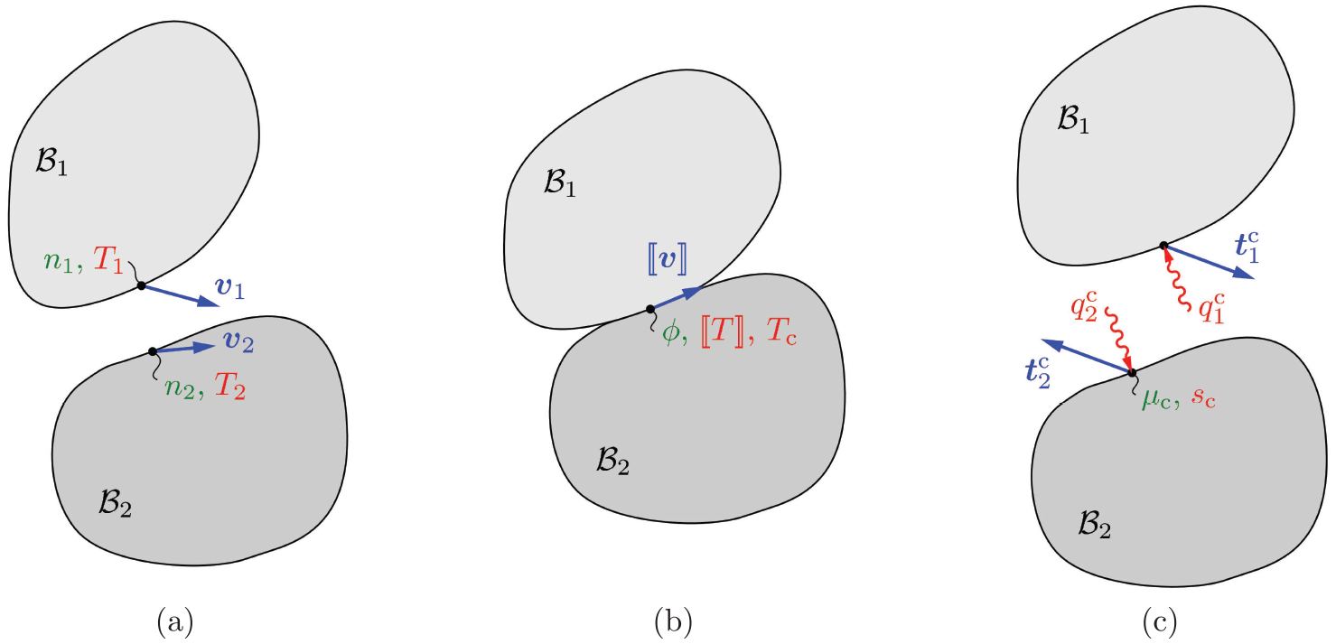
The two bodies can come into contact and interact mechanically, thermally, and chemically on their common contact surface ${\mathcal{S}}_{\mathrm{c}}:=\partial {\mathcal{B}}_1\cap \partial {\mathcal{B}}_2$ , see Figure 1. In case of long-range interaction, such as van der Waals adhesion, they may also interact when not in direct contact. In this case, interaction is considered to take place on the (non-touching) surfaces regions ${\mathcal{S}}_k\subset \partial {\mathcal{B}}_k$ . ¹

Figure 1.

Continuum contact description: (a) bodies before contact; (b) bodies in contact; (c) free-body diagram for contact. Here, $n_k$ , ${\mathit{v}}_k$ , and $T_k$ denote the bonding site density, velocity, and temperature, respectively, on the contact surface of body ${\mathcal{B}}_k$ ( $k=1,2$ ) at time $t$ . During contact, $\varphi$ denotes the degree of bonding, $[[\mathit{v}]]$ the velocity jump, $[[T]]$ the temperature jump, $T_{\mathrm{c}}$ the contact temperature, ${\mathit{t}}_k^{\mathrm{c}}$ the contact tractions, $q_k^{\mathrm{c}}$ the heat influx, ${\mu }_{\mathrm{c}}$ the chemical contact potential, and $s_{\mathrm{c}}$ the contact entropy. Here $T_{\mathrm{c}}$ and $s_{\mathrm{c}}$ are associated with an interfacial medium.

The deformation within each body is characterized by the deformation gradient

$$\begin{array}{c}{\mathit{F}}_k:=\frac{\partial {\mathit{x}}_k}{\partial {\mathit{X}}_k},\hfill \end{array}$$

(2)

from which various strain measures can be derived, such as the Green–Lagrange strain tensor

$$\begin{array}{c}{\mathit{E}}_k:=({\mathit{F}}_k^{\mathrm{T}}{\mathit{F}}_k-\mathbf{1})/2.\hfill \end{array}$$

(3)

The deformation generally contains elastic and inelastic contributions that lead to the additive strain decomposition ²

$$\begin{array}{c}{\mathit{E}}_k={\mathit{E}}_k^{\mathrm{e}}+{\mathit{E}}_k^{\mathrm{i}}.\hfill \end{array}$$

(4)

An example for an inelastic strain is thermal expansion. From ${\mathit{F}}_k$ also follows the quantity

$$\begin{array}{c}{J}_k:=det{\mathit{F}}_k,\hfill \end{array}$$

(5)

which governs the local volume change

$$\begin{array}{c}\mathrm{d}{v}_k=J_k\mathrm{d}{V}_k\hfill \end{array}$$

(6)

at ${\mathit{x}}_k\in {\mathcal{B}}_k$ between undeformed and deformed configuration. Similarly, the local surface area change

$$\begin{array}{c}\mathrm{d}{a}_k=J_{\mathrm{s}k}\mathrm{d}{A}_k\hfill \end{array}$$

(7)

at ${\mathit{x}}_k\in {\mathcal{S}}_k$ is governed by the quantity

$$\begin{array}{c}{J}_{\mathrm{s}k}:={det}_{\mathrm{s}}{\mathit{F}}_k,\hfill \end{array}$$

(8)

where $\underset{\mathrm{s}}{det}(\dots )$ is the surface determinant on ${\mathcal{S}}_k$ , see, e.g., [68].

Time-dependent deformation is characterized by the symmetric velocity gradient

$$\begin{array}{c}{\mathit{D}}_k:=(\nabla {\mathit{v}}_k+\nabla {\mathit{v}}_k^{\mathrm{T}})/2,\hfill \end{array}$$

(9)

also known as the rate of deformation tensor. The velocity also gives rise to the identities

$$\begin{array}{c}\frac{{\stackrel{·}{J}}_k}{J_k}=\mathrm{div}{\mathit{v}}_k\hfill \end{array}$$

(10)

and

$$\begin{array}{c}\frac{{\stackrel{·}{J}}_{\mathrm{s}k}}{J_{\mathrm{s}k}}={\mathrm{div}}_{\mathrm{s}}{\mathit{v}}_k,\hfill \end{array}$$

(11)

where ${\mathrm{div}}_{\mathrm{s}}(\dots )$ is the surface divergence on ${\mathcal{S}}_k$ .

Mechanical interaction between the two bodies is characterized by the gap vector

$$\begin{array}{c}\mathit{g}:={\mathit{x}}_2-{\mathit{x}}_1,\hfill \end{array}$$

(12)

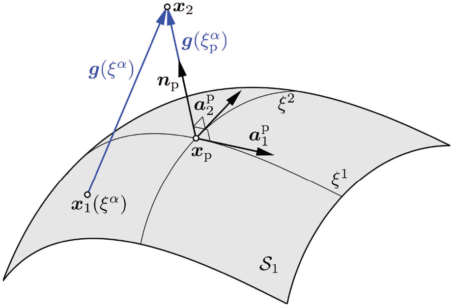
that is defined for all pairs ${\mathit{x}}_1\in {\mathcal{S}}_1$ and ${\mathit{x}}_2\in {\mathcal{S}}_2$ . Two cases have to be distinguished. (i) Both ${\mathit{x}}_1$ and ${\mathit{x}}_2$ are material points, a setting that is suitable for describing long-range interactions; or more generally (ii) one of the points is not necessarily a material point, a setting that arises when using a closest point projection suitable for short-range interactions. In the latter case, one surface, say ${\mathcal{S}}_1$ , is designated the so-called master surface, whereas the other, ${\mathcal{S}}_2$ , is designated the so-called slave surface [69]. The master surface is then used to define normal and tangential contact contributions. Therefore, the master point ${\mathit{x}}_1$ in (12) is determined as the closest point projection of slave point ${\mathit{x}}_2$ onto master surface ${\mathcal{S}}_1$ . Parameterizing ${\mathcal{S}}_1$ by the curvilinear surface coordinates ${\xi }^{\alpha }$ , $\alpha \in \{1,2\}$ , the closest projection point is given by

$$\begin{array}{c}{\mathit{x}}_{\mathrm{p}}:={\mathit{x}}_1({\xi }_{\mathrm{p}}^{\alpha },t),\hfill \end{array}$$

(13)

where ${\xi }_{\mathrm{p}}^{\alpha }$ is the value of ${\xi }^{\alpha }$ that solves the minimum distance problem

$$\begin{array}{c}\mathit{g}·{\mathit{a}}_{\alpha }=0.\hfill \end{array}$$

(14)

Here ${\mathit{a}}_{\alpha }:=\partial {\mathit{x}}_1/\partial {\xi }^{\alpha }$ ( $\alpha =1,2$ ) are tangent vectors of ${\mathcal{S}}_1$ , which at ${\mathit{x}}_{\mathrm{p}}$ are denoted ${\mathit{a}}_{\alpha }^{\mathrm{p}}$ , i.e., ${\mathit{a}}_{\alpha }^{\mathrm{p}}:={\mathit{a}}_{\alpha }({\xi }_{\mathrm{p}}^{\alpha },t)$ . Likewise ${\mathit{n}}_{\mathrm{p}}={\mathit{n}}_1({\xi }_{\mathrm{p}}^{\alpha },t)$ is the surface normal at ${\mathit{x}}_{\mathrm{p}}$ . The closest point projection is illustrated in Figure 2.

Figure 2.

Mechanical contact: computation of the contact gap $\mathit{g}$ via a closest point projection of slave point ${\mathit{x}}_2$ onto the master surface ${\mathcal{S}}_1$ .

The gap can be decomposed into its normal and tangential parts

$$\begin{array}{c}{g}_{\mathrm{n}}:=\mathit{g}·\mathit{n},{\mathit{g}}_{\mathrm{t}}:=\mathit{g}-g_{\mathrm{n}}\mathit{n},\hfill \end{array}$$

(15)

where the latter is zero at ${\mathit{x}}_{\mathrm{p}}$ . Hence, for contact $\mathit{g}=g_{\mathrm{n}}{\mathit{n}}_{\mathrm{p}}$ and $g_{\mathrm{n}}=0$ , so that

$$\begin{array}{c}\stackrel{·}{\mathit{g}}={\stackrel{·}{g}}_{\mathrm{n}}{\mathit{n}}_{\mathrm{p}}.\hfill \end{array}$$

(16)

Based on (12) and (13), the material time derivative of $\mathit{g}$ can also be written as

$$\begin{array}{c}\stackrel{·}{\mathit{g}}={\stackrel{·}{\mathit{x}}}_2-{\stackrel{·}{\mathit{x}}}_1-{\stackrel{·}{\xi }}_{\mathrm{p}}^{\alpha }{\mathit{a}}_{\alpha }^{\mathrm{p}},\hfill \end{array}$$

(17)

where, in agreement with definition (1), ${\stackrel{·}{\mathit{x}}}_1=\partial {\mathit{x}}_1/\partial t{|}_{{\xi }_{\mathrm{p}}^{\alpha }=\mathrm{fixed}}$ and ${\stackrel{·}{\xi }}_{\mathrm{p}}^{\alpha }=\partial {\xi }_{\mathrm{p}}^{\alpha }/\partial t{|}_{{\mathit{X}}_2=\mathrm{fixed}}$ . The latter part

$$\begin{array}{c}\stackrel{°}{{\mathit{g}}_{\mathrm{t}}}:={\stackrel{·}{\xi }}_{\mathrm{p}}^{\alpha }{\mathit{a}}_{\alpha }^{\mathrm{p}},\hfill \end{array}$$

(18)

(with summation implied over $\alpha$ and often denoted ${\mathcal{L}}_v{\mathit{g}}_{\mathrm{t}}$ ) is equal to the Lie derivative of the tangential gap vector [35]. Likewise (16) is equal to the Lie derivative of the normal gap vector. Here $\stackrel{°}{{\mathit{g}}_{\mathrm{t}}}$ is zero when ${\xi }_{\mathrm{p}}^{\alpha }$ is fixed (such that ${\stackrel{·}{\xi }}_{\mathrm{p}}^{\alpha }=0$ ), i.e., when ${\mathit{x}}_1$ is a material point as in case (i) above. In case (ii), $\stackrel{°}{{\mathit{g}}_{\mathrm{t}}}$ is equal to the relative tangential velocity between the two surfaces. Thus, ${\stackrel{·}{\xi }}_{\mathrm{p}}^{\alpha }=0$ also denotes the case of tangential sticking, while ${\stackrel{·}{\xi }}_{\mathrm{p}}^{\alpha }\ne 0$ characterizes tangential sliding. The sliding motion is irreversible and accumulates over time. Combining (16) and (17), one can identify the velocity jump

$$\begin{array}{c}[[\mathit{v}]]:={\mathit{v}}_2-{\mathit{v}}_1={\stackrel{·}{g}}_{\mathrm{n}}{\mathit{n}}_{\mathrm{p}}+\stackrel{°}{{\mathit{g}}_{\mathrm{t}}}=\stackrel{°}{\mathit{g}},\hfill \end{array}$$

(19)

and see that it is the Lie derivative of the total gap vector in case (ii). Even during sticking, it can be advantageous (see remark 2.2) to allow for (small) motion that is reversible upon unloading. This leads to the tangential velocity decomposition

$$\begin{array}{c}{\stackrel{·}{\xi }}_{\mathrm{p}}^{\alpha }={\stackrel{·}{\xi }}_{\mathrm{e}}^{\alpha }+{\stackrel{·}{\xi }}_{\mathrm{i}}^{\alpha },\hfill \end{array}$$

(20)

where ${\stackrel{·}{\xi }}_{\mathrm{e}}^{\alpha }$ captures the reversible (elastic) motion during sticking, while ${\stackrel{·}{\xi }}_{\mathrm{i}}^{\alpha }$ captures the irreversible (inelastic) motion during sliding. Plugging (20) into (19) yields

$$\begin{array}{c}[[\mathit{v}]]={\stackrel{°}{\mathit{g}}}_{\mathrm{e}}+{\stackrel{°}{\mathit{g}}}_{\mathrm{i}},\hfill \end{array}$$

(21)

where ${\stackrel{°}{\mathit{g}}}_{\mathrm{e}}:={\stackrel{·}{g}}_{\mathrm{n}}{\mathit{n}}_{\mathrm{p}}+{\stackrel{·}{\xi }}_{\mathrm{e}}^{\alpha }{\mathit{a}}_{\alpha }^{\mathrm{p}}$ characterizes normal contact and tangential sticking, whereas ${\stackrel{°}{\mathit{g}}}_{\mathrm{i}}:={\stackrel{·}{\xi }}_{\mathrm{i}}^{\alpha }{\mathit{a}}_{\alpha }^{\mathrm{p}}$ characterizes tangential sliding. Decomposition (21) is analogous to decomposition (4), making the contact kinematics analogous to the kinematics of the bodies. It contains (19) for the case ${\stackrel{·}{\xi }}_{\mathrm{e}}^{\alpha }=0$ . Expressions for ${\stackrel{·}{g}}_{\mathrm{n}}$ and ${\stackrel{·}{\xi }}_{\mathrm{p}}^{\alpha }$ can be found, e.g., in [35].

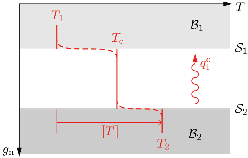
Thermal contact is characterized by the temperature jump between surface points ${\mathit{x}}_1$ and ${\mathit{x}}_2$ ,

$$\begin{array}{c}[[T]]:=T_2-T_1,\hfill \end{array}$$

(22)

also denoted as the thermal gap [13], and the contact temperature $T_{\mathrm{c}}$ that is associated with an interfacial medium, e.g., a lubricant or wear particles, see Figure 3. It is assumed that this medium is very thin, such that $T_{\mathrm{c}}$ is constant through the thickness of the medium and can only vary along the surface.

Figure 3.

Thermal contact: assumed temperature profile $T(g_{\mathrm{n}})$ across the contact interface (along coordinate $g_{\mathrm{n}}$ ). Thermal contact between two bodies is characterized by the temperature jump $[[T]]:=T_2-T_1$ and the contact temperature $T_{\mathrm{c}}$ associated with an interfacial medium. Here $[[T]]$ leads to the transfer heat flux $q_{\mathrm{t}}^{\mathrm{c}}=h[[T]]$ identified in Section 4.3.

In order to characterize chemical contact, the bonding state variable $\varphi =\varphi (\mathit{x},t)$ is introduced on the contact surface, as discussed in the following section. It varies between $\varphi =0$ for no bonding and $\varphi =1$ for full bonding, and can be associated with a chemical gap (e.g., defined as $1-\varphi$ ).

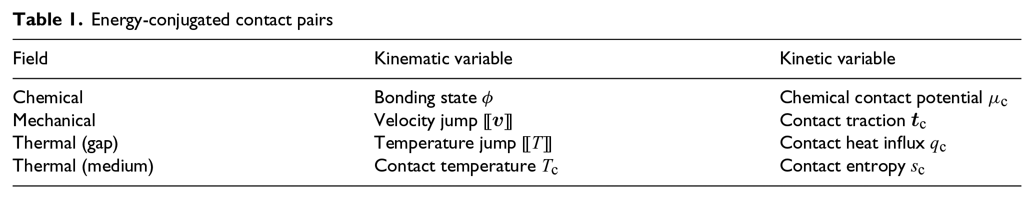
Table 1 summarizes the kinematic contact variables and their corresponding kinetic counterparts that will be discussed in later sections.

Table 1.

Energy-conjugated contact pairs

Field	Kinematic variable	Kinetic variable
Chemical	Bonding state $\varphi$	Chemical contact potential ${\mu }_{\mathrm{c}}$
Mechanical	Velocity jump $[[\mathit{v}]]$	Contact traction ${\mathit{t}}_{\mathrm{c}}$
Thermal (gap)	Temperature jump $[[T]]$	Contact heat influx $q_{\mathrm{c}}$
Thermal (medium)	Contact temperature $T_{\mathrm{c}}$	Contact entropy $s_{\mathrm{c}}$

Remark 2.1. Apart from the tangential sticking constraint ${\stackrel{·}{\xi }}_{\mathrm{p}}^{\alpha }=0$ , there is also the normal contact constraint $g_{\mathrm{n}}\ge 0$ . Normal and tangential contact are usually treated separately in most friction algorithms, but there are also unified approaches directly based on the gap vector $\mathit{g}$ , see, e.g., [70, 71]. Such an approach is also taken in the following sections.

Remark 2.2. There are reasons for relaxing the contact constraints $g_{\mathrm{n}}\ge 0$ and ${\stackrel{·}{\xi }}_{\mathrm{p}}^{\alpha }=0$ . One is to use a penalty regularization, which is typically simpler to implement than the exact constraint enforcement. Another is to use the elastic gap ${\mathit{g}}_{\mathrm{e}}$ to capture the elastic deformation of (microscale) surface asperities during contact. In both cases ${\mathit{g}}_{\mathrm{e}}$ is non-zero (but typically small) during contact.

Remark 2.3. The designation into master and slave surfaces introduces a bias in the contact formulation that can affect the accuracy and robustness of computational methods. The bias can be removed if alternating master/slave designations are used, as is done for 3D friction in [72, 73].

Remark 2.4. As shown previously, the Lie derivatives $\stackrel{°}{\mathit{g}}$ and ${\stackrel{°}{\mathit{g}}}_e$ only contain the relative changes of the normal and tangential gap. They do not contain the basis changes ${\stackrel{·}{\mathit{n}}}_{\mathrm{p}}$ and ${\stackrel{·}{\mathit{a}}}_{\alpha }^{\mathrm{p}}$ . This makes the Lie derivative objective and a suitable quantity for the constitutive modeling [67], see Section 4.1.

3. Balance laws

This section derives the chemical, mechanical, and thermal balance laws for a generally coupled two-body system. The resulting equations turn out to be in the same form as the known relations for chemical reactions [74] and thermo-mechanical contact [67]. The novelty here lies in establishing their coupling and highlighting the similarities among the chemical, mechanical, and thermal contact equations. The derivation is based on the following three mathematical ingredients. The first is Reynolds’ transport theorem for volume integrals,

$$\begin{array}{c}\frac{\mathrm{d}}{\mathrm{d}t}{\int }_{{\mathcal{B}}_k}\dots \mathrm{d}{v}_k={\int }_{{\mathcal{B}}_k}((\stackrel{·}{\dots })+\mathrm{div}{\mathit{v}}_k(\dots ))\mathrm{d}{v}_k.\hfill \end{array}$$

(23)

It follows from substituting (6) on the left, using the product rule, and then applying (10). Applied to surfaces, Reynolds’ transport theorem simply adapts to

$$\begin{array}{c}\frac{\mathrm{d}}{\mathrm{d}t}{\int }_{{\mathcal{S}}_k}\dots \mathrm{d}{a}_k={\int }_{{\mathcal{S}}_k}((\stackrel{·}{\dots })+{\mathrm{div}}_{\mathrm{s}}{\mathit{v}}_k(\dots ))\mathrm{d}{a}_k.\hfill \end{array}$$

(24)

It follows from substituting (7) on the left, using the product rule, and then applying (11).

The second ingredient is the divergence theorem,

$$\begin{array}{c}{\int }_{\partial {\mathcal{B}}_k}\dots {\mathit{n}}_k\mathrm{d}{a}_k={\int }_{{\mathcal{B}}_k}\mathrm{div}(\dots )\mathrm{d}{v}_k,\hfill \end{array}$$

(25)

where ${\mathit{n}}_k$ is the outward normal vector of boundary $\partial {\mathcal{B}}_k$ . The third ingredient is the localization theorem,

$$\begin{array}{c}{\int }_{\mathcal{P}}\dots \mathrm{d}v=0\mathrm{for}\mathrm{all}\mathcal{P}\subset \mathcal{B}\iff \dots =0\mathrm{for}\mathrm{all}\mathit{x}\in \mathcal{B},\hfill \end{array}$$

(26)

that can be equally applied to surface integrals.

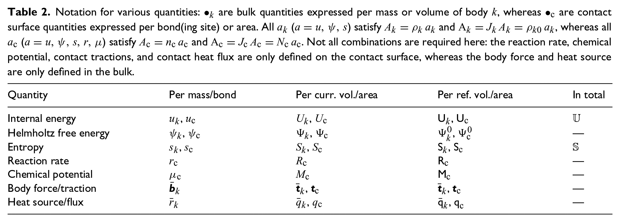
Some of the field quantities appearing in the following balance laws can be expressed per mass, bonding site, current volume, current area, reference volume, or reference area. The notation distinguishing these options is summarized in Table 2.

Table 2.

Notation for various quantities: ${•}_k$ are bulk quantities expressed per mass or volume of body $k$ , whereas ${•}_{\mathrm{c}}$ are contact surface quantities expressed per bond(ing site) or area. All $a_k$ ( $a=u,\psi ,s$ ) satisfy $A_k={\rho }_k{a}_k$ and ${\mathrm{A}}_k=J_k{A}_k={\rho }_{k0}{a}_k$ , whereas all $a_{\mathrm{c}}$ ( $a=u,\psi ,s,r,\mu$ ) satisfy $A_{\mathrm{c}}=n_{\mathrm{c}}{a}_{\mathrm{c}}$ and ${\mathrm{A}}_{\mathrm{c}}=J_{\mathrm{c}}{A}_{\mathrm{c}}=N_{\mathrm{c}}{a}_{\mathrm{c}}$ . Not all combinations are required here: the reaction rate, chemical potential, contact tractions, and contact heat flux are only defined on the contact surface, whereas the body force and heat source are only defined in the bulk.

Quantity	Per mass/bond	Per curr. vol./area	Per ref. vol./area	In total
Internal energy	$u_k$ , $u_{\mathrm{c}}$	$U_k$ , $U_{\mathrm{c}}$	$U_k$ , $U_{\mathrm{c}}$	$\mathbb{U}$
Helmholtz free energy	${\psi }_k$ , ${\psi }_{\mathrm{c}}$	${\mathrm{\Psi }}_k$ , ${\mathrm{\Psi }}_{\mathrm{c}}$	${\mathrm{\Psi }}_k^0$ , ${\mathrm{\Psi }}_{\mathrm{c}}^0$	—
Entropy	$s_k$ , $s_{\mathrm{c}}$	$S_k$ , $S_{\mathrm{c}}$	$S_k$ , $S_{\mathrm{c}}$	$\mathbb{S}$
Reaction rate	$r_{\mathrm{c}}$	$R_{\mathrm{c}}$	$R_{\mathrm{c}}$	—
Chemical potential	${\mu }_{\mathrm{c}}$	$M_{\mathrm{c}}$	$M_{\mathrm{c}}$	—
Body force/traction	${\overline{\mathit{b}}}_k$	${\overline{\mathit{t}}}_k$ , ${\mathit{t}}_{\mathrm{c}}$	${\overline{\mathit{t}}}_k$ , ${\mathit{t}}_{\mathrm{c}}$	—
Heat source/flux	${\overline{r}}_k$	${\overline{q}}_k$ , $q_{\mathrm{c}}$	$q_k$ , $q_{\mathrm{c}}$	—

3.1. Conservation of mass and bonding sites

Assuming no mass sources, the mass balance of each body is given by the statement

$$\begin{array}{c}\frac{\mathrm{d}}{\mathrm{d}t}{\int }_{{\mathcal{P}}_k}{\rho }_k\mathrm{d}{v}_k=0\mathrm{for}\mathrm{all}{\mathcal{P}}_k\subset {\mathcal{B}}_k.\hfill \end{array}$$

(27)

Applying (23) and (26), this leads to the local balance law

$$\begin{array}{c}{\stackrel{·}{\rho }}_k+{\rho }_k\mathrm{div}{\mathit{v}}_k=0\mathrm{for}\mathrm{all}{\mathit{x}}_k\in {\mathcal{B}}_k.\hfill \end{array}$$

(28)

Owing to (10), this ODE is solved by ${\rho }_k={\rho }_{0k}/J_k$ , where ${\rho }_{0k}:={\rho }_k{|}_{t=0}$ is the initial mass density.

In order to model chemical bonding, the interacting surfaces are considered to have a certain bonding site density $n_k$ (the number of bonding sites per current area) composed of bonded sites and unbonded sites, i.e.,

$$\begin{array}{c}{n}_k=n_k^{\mathrm{b}}+n_k^{\mathrm{ub}}.\hfill \end{array}$$

(29)

The number of bonding sites is considered to be conserved, i.e.,

$$\begin{array}{c}\frac{\mathrm{d}}{\mathrm{d}t}{\int }_{{\mathcal{P}}_k}{n}_k\mathrm{d}{a}_k=0\mathrm{for}\mathrm{all}{\mathcal{P}}_k\subset {\mathcal{S}}_k,\hfill \end{array}$$

(30)

implying

$$\begin{array}{c}{\stackrel{·}{n}}_k+n_k{\mathrm{div}}_{\mathrm{s}}{\mathit{v}}_k=0\mathrm{for}\mathrm{all}{\mathit{x}}_k\in {\mathcal{S}}_k,\hfill \end{array}$$

(31)

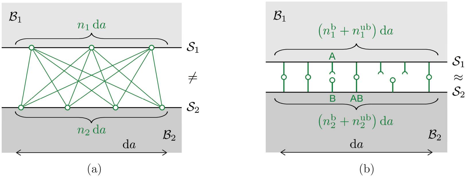
due to (24) and (26). Owing to (11), this ODE is solved by $n_k=N_k/J_{\mathrm{s}k}$ , where $N_k:=n_k{|}_{t=0}$ is the initial bonding site density. Two cases are considered in the following, see Figure 4. (a) Long-range interaction ³ (between non-touching surfaces), where each bonding site on one surface can interact with all other bonding sites on the other surface. (b) Short-range interactions (between very close or even touching surfaces), where each bonding site on one surface can only bond to a single bonding site on the other surface.

Figure 4.

Chemical contact interactions. (a) Long-range interactions between all bonding sites (e.g., molecules) of two non-touching surfaces. Here $n_1\mathrm{d}a=3$ and $n_2\mathrm{d}a=4$ . (b) Short-range bonding reactions between neighboring bonding sites A and B of two close surfaces. Here $n_1^{\mathrm{b}}\mathrm{d}a=n_2^{\mathrm{b}}\mathrm{d}a=4$ bonds have formed, whereas $n_1^{\mathrm{ub}}\mathrm{d}a=3$ and $n_2^{\mathrm{ub}}\mathrm{d}a=2$ sites are unbonded.

In the first case, we assume $n_k^{\mathrm{ub}}=0$ such that $n_k=n_k^{\mathrm{b}}$ . Then no further equation is needed for $n_k^{\mathrm{b}}$ . An example are van der Waals interactions described by the Lennard–Jones potential discussed in Section 5.3. In the second case, discussed in the remainder of this section, further equations are needed for $n_k^{\mathrm{b}}$ . As the total number of bonded sites is the same on both surfaces in this case, we must have

$${\int }_{{\mathcal{S}}_1}{n}_1^{\mathrm{b}}\mathrm{d}{a}_1={\int }_{{\mathcal{S}}_2}{n}_2^{\mathrm{b}}\mathrm{d}{a}_2.$$

(32)

If the two surfaces are very close, ${\mathcal{S}}_1\approx {\mathcal{S}}_2$ can be replaced by a common reference surface ${\mathcal{S}}_{\mathrm{c}}$ . Equation (32) then implies that $n_1^{\mathrm{b}}=n_2^{\mathrm{b}}=:n_{\mathrm{b}}$ due to localization (because (32) is still true for any subregion ${\mathcal{P}}_{\mathrm{c}}\subset {\mathcal{S}}_{\mathrm{c}}$ ). This case is considered in the following.

The evolution of $n_{\mathrm{b}}$ is described by the chemical reaction

$$\begin{array}{c}\mathrm{A}+\mathrm{B}\rightleftharpoons \mathrm{AB},\hfill \end{array}$$

(33)

where AB denotes the bond, whereas A and B are its components on the two surfaces prior to bonding, see Figure 4(b). The bonding reaction is characterized by the reaction rate

$$\begin{array}{c}{R}_{\mathrm{c}}=\overrightarrow{R_{\mathrm{c}}}-\overleftarrow{R_{\mathrm{c}}},\hfill \end{array}$$

(34)

composed of the bonding reaction rate $\overrightarrow{R_{\mathrm{c}}}$ (forward reaction) and the debonding reaction rate $\overleftarrow{R_{\mathrm{c}}}$ (backward reaction). An example for these is discussed in Section 5.7. Given $R_{\mathrm{c}}$ , the balance law for the bonded sites (considering no surface diffusion) then follows as [75]

$$\begin{array}{c}\frac{\mathrm{d}}{\mathrm{d}t}{\int }_{{\mathcal{P}}_{\mathrm{c}}}{n}_{\mathrm{b}}\mathrm{d}a={\int }_{{\mathcal{P}}_{\mathrm{c}}}{R}_{\mathrm{c}}\mathrm{d}a\mathrm{for}\mathrm{all}{\mathcal{P}}_{\mathrm{c}}\subset {\mathcal{S}}_{\mathrm{c}},\hfill \end{array}$$

(35)

which gives

$$\begin{array}{c}{\stackrel{·}{n}}_{\mathrm{b}}+n_{\mathrm{b}}{\mathrm{div}}_{\mathrm{s}}{\mathit{v}}_{\mathrm{c}}=R_{\mathrm{c}}\mathrm{for}\mathrm{all}{\mathit{x}}_{\mathrm{c}}\in {\mathcal{S}}_{\mathrm{c}},\hfill \end{array}$$

(36)

where ${\mathit{v}}_{\mathrm{c}}:={\mathit{v}}_1={\mathit{v}}_2$ is the common velocity required to enable chemical bonding. For the unbonded sites on the two surfaces, we have the two balance laws

$$\begin{array}{c}\frac{\mathrm{d}}{\mathrm{d}t}{\int }_{{\mathcal{P}}_k}{n}_k^{\mathrm{ub}}\mathrm{d}{a}_k=-{\int }_{{\mathcal{P}}_k}{R}_{\mathrm{c}}\mathrm{d}{a}_k\mathrm{for}\mathrm{all}{\mathcal{P}}_k\subset {\mathcal{S}}_k,k=1,2,\hfill \end{array}$$

(37)

leading to

$$\begin{array}{c}{\stackrel{·}{n}}_k^{\mathrm{ub}}+n_k^{\mathrm{ub}}{\mathrm{div}}_{\mathrm{s}}{\mathit{v}}_k=-R_{\mathrm{c}}\mathrm{for}\mathrm{all}{\mathit{x}}_k\in {\mathcal{S}}_k,\hfill \end{array}$$

(38)

where still ${\mathit{v}}_1={\mathit{v}}_2$ (as long as $n_{\mathrm{b}}>0$ ). Summing (36) and (38) leads to (31), and so one equation (for each $k$ ) is redundant.

For convenience, the non-dimensional phase field

$$\begin{array}{c}\varphi :=\frac{n_{\mathrm{b}}}{n_{\mathrm{c}}},0\le \varphi \le 1,\hfill \end{array}$$

(39)

is introduced, where $n_{\mathrm{c}}$ is the reference value for the bonding site density, either picked as $n_{\mathrm{c}}=n_1$ , in case surface 1 is taken as reference, or $n_{\mathrm{c}}=n_2$ , in case surface 2 is taken as reference. ⁴ Then (36) can be rewritten into

$$n_{\mathrm{c}}\stackrel{·}{\varphi }=R_{\mathrm{c}}\mathrm{for}\mathrm{all}{\mathit{x}}_{\mathrm{c}}\in {\mathcal{S}}_{\mathrm{c}},$$

(40)

using (31). Equation (40) is the evolution law for the chemical contact state.

Remark 3.1. As we are focusing on solids, the derivation of (40) assumes no surface mobility (or diffusion) of the bonds. In the context of fluidic membranes, the surface mobility of bonds is usually accounted for, see, e.g., [76, 77].

Remark 3.2. In the derivation leading up to (31), ${\mathit{v}}_1={\mathit{v}}_2$ has been used. However, it suffices to assume that the time scale of chemical reactions is much smaller than the timescale of sliding, such that the two reacting surfaces can be assumed stationary with respect to one another.

3.2. Momentum balance

The linear momentum balance for the entire two-body system is given by

$$\begin{array}{c}\sum _{k=1}^2\frac{\mathrm{d}}{\mathrm{d}t}{\int }_{{\mathcal{B}}_k}{\rho }_k{\mathit{v}}_k\mathrm{d}{v}_k=\sum _{k=1}^2[{\int }_{{\mathcal{B}}_k}{\rho }_k{\overline{\mathit{b}}}_k\mathrm{d}{v}_k+{\int }_{{\partial }_t{\mathcal{B}}_k}{\overline{\mathit{t}}}_k\mathrm{d}{a}_k],\hfill \end{array}$$

(41)

where ${\overline{\mathit{b}}}_k$ and ${\overline{\mathit{t}}}_k$ are prescribed body forces and surface tractions. The latter are prescribed on the Neumann boundary ${\partial }_t{\mathcal{B}}_k\subset \partial {\mathcal{B}}_k$ that is disjoint from contact surface ${\mathcal{S}}_k$ . The bonding events, described by Eq. (40), are not considered to affect the momentum of the system.

If the two bodies are cut apart, the additional contact interaction traction ${\mathit{t}}_k^{\mathrm{c}}$ needs to be taken into account on the interface (see Figure 1). The individual momentum balance for every part ${\mathcal{P}}_k\subset {\mathcal{B}}_k$ ( $k=1,2$ ) then reads

$$\begin{array}{c}\frac{\mathrm{d}}{\mathrm{d}t}{\int }_{{\mathcal{P}}_k}{\rho }_k{\mathit{v}}_k\mathrm{d}{v}_k={\int }_{{\mathcal{P}}_k}{\rho }_k{\overline{\mathit{b}}}_k\mathrm{d}{v}_k+{\int }_{\partial {\mathcal{P}}_k}{\mathit{t}}_k\mathrm{d}{a}_k\mathrm{for}\mathrm{all}{\mathcal{P}}_k\subset {\mathcal{B}}_k,\hfill \end{array}$$

(42)

where ${\mathit{t}}_k$ is the traction on the surface $\partial {\mathcal{P}}_k$ that contains the cases

$$\begin{array}{c}{\mathit{t}}_k={\overline{\mathit{t}}}_k\mathrm{on}{\partial }_t{\mathcal{B}}_k,\hfill \\ \multicolumn{1}{c}{{\mathit{t}}_k={\mathit{t}}_k^{\mathrm{c}}\mathrm{on}{\mathcal{S}}_k.}\end{array}$$

(43)

Applying (23), (25), and (26) leads to the corresponding local form

$${\rho }_k{\stackrel{·}{\mathit{v}}}_k=\mathrm{div}{\mathit{\sigma }}_{\mathrm{}k}+{\rho }_k{\overline{\mathit{b}}}_k\mathrm{for}\mathrm{all}{\mathit{x}}_k\in {ℬ}_k,$$

(44)

where ${\mathit{\sigma }}_k$ is the Cauchy stress at ${\mathit{x}}_k$ that is defined by the formula

$$\begin{array}{c}{\mathit{\sigma }}_k{\mathit{n}}_k={\mathit{t}}_k.\hfill \end{array}$$

(45)

Using (42), Equation (41) implies

$${\int }_{{\mathcal{S}}_1}{\mathit{t}}_1^{\mathrm{c}}\mathrm{d}{a}_1+{\int }_{{\mathcal{S}}_2}{\mathit{t}}_2^{\mathrm{c}}\mathrm{d}{a}_2=\mathbf{0}.$$

(46)

This simply states that the net contact forces are in equilibrium. It is the corresponding statement to (32) for mechanical contact. If the two surfaces touch, i.e., ${\mathcal{S}}_1\approx {\mathcal{S}}_2=:{\mathcal{S}}_{\mathrm{c}}$ and $\mathrm{d}{a}_1\approx \mathrm{d}{a}_2$ , Equation (46) implies that

$${\mathit{t}}_1^{\mathrm{c}}=-{\mathit{t}}_2^{\mathrm{c}}=:{\mathit{t}}_{\mathrm{c}}\mathrm{for}\mathrm{all}{\mathit{x}}_{\mathrm{c}}\in {\mathcal{S}}_{\mathrm{c}}.$$

(47)

Hence, there is no jump in the contact traction. Such a jump only arises if an interface stress (e.g., surface tension) is considered.

The angular momentum balances for the individual bodies and the entire two-body system can be written down analogously to (42) and (41), respectively. As long as no distributed body and surface moments are considered, the angular momentum balance of each body has the well-known consequence ${\mathit{\sigma }}_k^{\mathrm{T}}=$ ${\mathit{\sigma }}_k$ (see [78]), whereas global angular momentum balance implies

$${\int }_{{\mathcal{S}}_1}{\mathit{x}}_1\times {\mathit{t}}_1^{\mathrm{c}}\mathrm{d}{a}_1+{\int }_{{\mathcal{S}}_2}{\mathit{x}}_2\times {\mathit{t}}_2^{\mathrm{c}}\mathrm{d}{a}_2=\mathbf{0},$$

(48)

analogously to (46). This statement is relevant for separated surfaces ( ${\mathcal{S}}_1\ne {\mathcal{S}}_2$ ), but, in the case of touching surfaces ( ${\mathcal{S}}_1\approx {\mathcal{S}}_2$ ), it leads to the already known traction equivalence (47) at common contact points ${\mathit{x}}_1={\mathit{x}}_2$ .

Remark 3.3. In (47) the master surface ${\mathcal{S}}_1$ is taken as reference surface for defining the reference traction ${\mathit{t}}_{\mathrm{c}}$ , which is commonly done in mechanical contact formulations [35]. In case of chemical and thermal contact, however, the two possible choices $n_{\mathrm{c}}=n_1$ or $n_{\mathrm{c}}=n_2$ for the reference bonding site density introduced in (39) are maintained in this treatment.

3.3. Energy balance

The energy balance for the entire two-body system is

$$\begin{array}{c}\frac{\mathrm{d}\mathbb{E}}{\mathrm{d}t}=\sum _{k=1}^2[{\int }_{{\mathcal{B}}_k}{\rho }_k{\overline{r}}_k\mathrm{d}{v}_k+{\int }_{{\partial }_q{\mathcal{B}}_k}{\overline{q}}_k\mathrm{d}{a}_k+{\int }_{{\mathcal{B}}_k}{\rho }_k{\mathit{v}}_k·{\overline{\mathit{b}}}_k\mathrm{d}{v}_k+{\int }_{{\partial }_t{\mathcal{B}}_k}{\mathit{v}}_k·{\overline{\mathit{t}}}_k\mathrm{d}{a}_k],\hfill \end{array}$$

(49)

where the total energy in the system,

$$\begin{array}{c}\mathbb{E}=\mathbb{K}+\mathbb{U},\hfill \end{array}$$

(50)

is given by the kinetic energy

$$\begin{array}{c}\mathbb{K}=\frac{1}{2}{\int }_{{\mathcal{B}}_1}{\rho }_1{\mathit{v}}_1·{\mathit{v}}_1\mathrm{d}{v}_1+\frac{1}{2}{\int }_{{\mathcal{B}}_2}{\rho }_2{\mathit{v}}_2·{\mathit{v}}_2\mathrm{d}{v}_2\hfill \end{array}$$

(51)

and the internal energy

$$\begin{array}{c}\mathbb{U}={\int }_{{\mathcal{B}}_1}{\rho }_1{u}_1\mathrm{d}{v}_1+{\int }_{{\mathcal{B}}_2}{\rho }_2{u}_2\mathrm{d}{v}_2+{\mathbb{U}}_{\mathrm{c}},\hfill \end{array}$$

(52)

which accounts for the individual energies $u_k=u_k({\mathit{x}}_k)$ in ${\mathcal{B}}_k$ and the contact energy ${\mathbb{U}}_{\mathrm{c}}$ . Here ${\mathbb{U}}_{\mathrm{c}}$ can describe long-range surface interactions, as discussed in Remark 3.6, or it can correspond to the energy of a third medium residing in the contact interface, e.g., a thin film of lubricants or wear particles. In the latter case, assuming a sufficiently thin film, ${\mathbb{U}}_{\mathrm{c}}$ can be expressed as the surface integral

$$\begin{array}{c}{\mathbb{U}}_{\mathrm{c}}:={\int }_{{\mathcal{S}}_{\mathrm{c}}}{n}_{\mathrm{c}}{u}_{\mathrm{c}}\mathrm{d}a,\hfill \end{array}$$

(53)

where $u_{\mathrm{c}}$ is the contact energy per bonding site on contact surface ${\mathcal{S}}_{\mathrm{c}}$ . ⁵ Further, ${\overline{r}}_k$ and ${\overline{q}}_k$ in (49) denote external heat sources in ${\mathcal{B}}_k$ and external heat influxes on ${\partial }_q{\mathcal{B}}_k\subset \partial {\mathcal{B}}_k$ , respectively. The Neumann boundary ${\partial }_q{\mathcal{B}}_k$ is considered disjoint from contact surface ${\mathcal{S}}_k$ . An external heat source on the interface is not required here. As we show later, the present setup already accounts for the heat from interfacial friction and interfacial reactions.

If the two bodies are cut apart, the additional contact heat influx $q_k^{\mathrm{c}}$ needs to be taken into account on the interface (see Figure 1), leading to the individual energy balance for each body

$$\begin{array}{c}\frac{\mathrm{d}}{\mathrm{d}t}{\int }_{{\mathcal{P}}_k}{\rho }_k{e}_k\mathrm{d}{v}_k={\int }_{{\mathcal{P}}_k}{\rho }_k{\overline{r}}_k\mathrm{d}{v}_k+{\int }_{\partial {\mathcal{P}}_k}{q}_k\mathrm{d}{a}_k\hfill \\ \multicolumn{1}{c}{+{\int }_{{\mathcal{P}}_k}{\mathit{v}}_k·{\rho }_k{\overline{\mathit{b}}}_k\mathrm{d}{v}_k+{\int }_{\partial {\mathcal{P}}_k}{\mathit{v}}_k·{\mathit{t}}_k\mathrm{d}{a}_k\mathrm{for}\mathrm{all}{\mathcal{P}}_k\subset {\mathcal{B}}_k,}\end{array}$$

(54)

where $e_k:=u_k+{\mathit{v}}_k·{\mathit{v}}_k/2$ and ${\mathit{t}}_k$ satisfies (43). Further, $q_k$ is the heat influx on surface $\partial {\mathcal{P}}_k$ that contains the cases

$$\begin{array}{c}{q}_k={\overline{q}}_k\mathrm{on}{\partial }_q{\mathcal{B}}_k,\hfill \\ \multicolumn{1}{c}{q_k=q_k^{\mathrm{c}}\mathrm{on}{\mathcal{S}}_k.}\end{array}$$

(55)

Introducing the heat flux vector ${\mathit{q}}_k$ at ${\mathit{x}}_k\in {\mathcal{B}}_k$ that is defined by Stokes formula

$$\begin{array}{c}-{\mathit{q}}_k·{\mathit{n}}_k=q_k,\hfill \end{array}$$

(56)

and using (45), the divergence theorem (25) can be applied to obtain

$$\begin{array}{c}{\int }_{\partial {\mathcal{P}}_k}{q}_k\mathrm{d}{a}_k=-{\int }_{{\mathcal{P}}_k}\mathrm{div}{\mathit{q}}_k\mathrm{d}{v}_k\hfill \end{array}$$

(57)

and

$$\begin{array}{c}{\int }_{\partial {\mathcal{P}}_k}{\mathit{v}}_k·{\mathit{t}}_k\mathrm{d}{a}_k={\int }_{{\mathcal{P}}_k}({\mathit{v}}_k·\mathrm{div}{\mathit{\sigma }}_k+{\mathit{\sigma }}_k:{\mathit{D}}_k)\mathrm{d}{v}_k,\hfill \end{array}$$

(58)

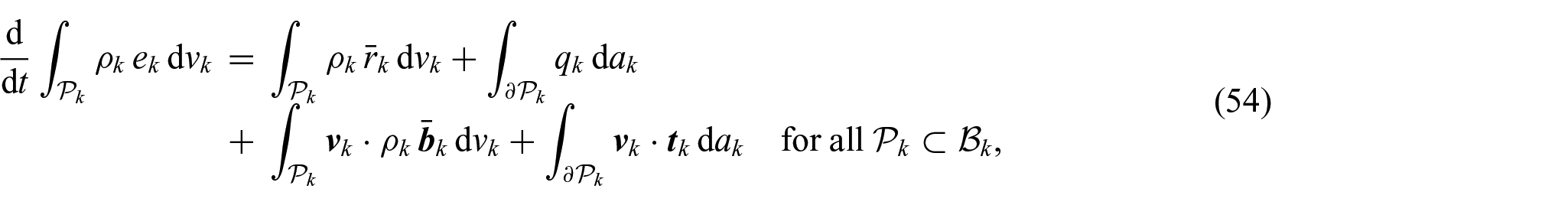
where ${\mathit{D}}_k$ is the symmetric velocity gradient from (9). Using (23), (26), and (44), the local form of (54) thus becomes

$${\rho }_k{\stackrel{·}{u}}_k={\rho }_k{\overline{r}}_k-\mathrm{div}{\mathit{q}}_k+{\mathit{\sigma }}_{\mathrm{}k}:{\mathit{D}}_k\mathrm{for}\mathrm{all}{\mathit{x}}_k\in {ℬ}_k.$$

(59)

With this and (44), the combined balance statement (49) implies

$${\stackrel{·}{\mathbb{U}}}_{\mathrm{c}}+{\int }_{{\mathcal{S}}_1}(q_1^{\mathrm{c}}+{\mathit{t}}_1^{\mathrm{c}}\cdot {\mathit{v}}_1)\mathrm{d}{a}_1+{\int }_{{\mathcal{S}}_2}(q_2^{\mathrm{c}}+{\mathit{t}}_2^{\mathrm{c}}\cdot {\mathit{v}}_2)\mathrm{d}{a}_2=0,$$

(60)

which is the corresponding statement to (32) and (46) for thermal contact. Here

$$\begin{array}{c}{\stackrel{·}{\mathbb{U}}}_{\mathrm{c}}={\int }_{{\mathcal{S}}_{\mathrm{c}}}{n}_{\mathrm{c}}{\stackrel{·}{u}}_{\mathrm{c}}\mathrm{d}a,\hfill \end{array}$$

(61)

follows from (53) for bonding site conservation (30). If the two surfaces are very close or even touch, i.e., ${\mathcal{S}}_1\approx {\mathcal{S}}_2=:{\mathcal{S}}_{\mathrm{c}}$ and $\mathrm{d}{a}_1\approx \mathrm{d}{a}_2$ (i.e., for very thin interfacial media), this implies that (because ${\mathcal{S}}_{\mathrm{c}}$ can be considered an arbitrary subregion of the contact surface)

$$n_{\mathrm{c}}{\stackrel{·}{u}}_{\mathrm{c}}+q_1^{\mathrm{c}}+q_2^{\mathrm{c}}+{\mathit{t}}_{\mathrm{c}}\cdot ({\mathit{v}}_1-{\mathit{v}}_2)=0\mathrm{for}\mathrm{all}{\mathit{x}}_{\mathrm{c}}\in {\mathcal{S}}_{\mathrm{c}},$$

(62)

due to (47). Equation (62) states that the energy rate ${\stackrel{·}{u}}_{\mathrm{c}}$ and the mechanical contact power ${\mathit{t}}_{\mathrm{c}}·({\mathit{v}}_1-{\mathit{v}}_2)$ cause the heat influxes $q_k^{\mathrm{c}}$ on ${\mathcal{S}}_k$ . Equation (62) is equivalent to (6.63) of Laursen [67]. ⁶

Remark 3.4. Using (21), the contact power becomes

$$\begin{array}{c}{\mathit{t}}_{\mathrm{c}}·({\mathit{v}}_1-{\mathit{v}}_2)={\mathit{t}}_{\mathrm{c}}·{\stackrel{°}{\mathit{g}}}_{\mathrm{e}}+{\mathit{t}}_{\mathrm{c}}·{\stackrel{°}{\mathit{g}}}_{\mathrm{i}},\hfill \end{array}$$

(63)

showing that it contains elastic and inelastic contributions associated with sticking and sliding, respectively. The first is associated with energy stored in the contact interface (defined by (82), later). This energy vanishes for an exact enforcement of sticking ( ${\mathit{g}}_{\mathrm{e}}=\mathit{0}$ ). The second contribution causes dissipation, which is also zero in the case of sticking (because ${\stackrel{°}{\mathit{g}}}_{\mathrm{i}}=\mathit{0}$ ) and in case of frictionless sliding (because ${\mathit{t}}_{\mathrm{c}}\perp {\stackrel{°}{\mathit{g}}}_{\mathrm{i}}$ ). In principle, the second contribution could also contain stored energy. In the context of plasticity such a stored energy occurs for hardening [79]. However, this is not considered here.

Remark 3.5. Note that in contrast to the contact tractions governed by (47), the contact heat flux according to (62) can have a jump across the interface. This has also been recently explored by [80].

Remark 3.6. For long-range interactions between two surfaces, ${\mathbb{U}}_{\mathrm{c}}$ can be written as ⁷

$$\begin{array}{c}{\mathbb{U}}_{\mathrm{c}}:={\int }_{{\mathcal{S}}_1}{\int }_{{\mathcal{S}}_2}{n}_1{n}_2{u}_{12}\mathrm{d}{a}_2\mathrm{d}{a}_1,\hfill \end{array}$$

(64)

where $u_{12}=u_{12}({\mathit{x}}_1,{\mathit{x}}_2)$ is an interaction energy defined between points on the two surfaces. For bonding site conservation (30) this leads to

$$\begin{array}{c}{\stackrel{·}{\mathbb{U}}}_{\mathrm{c}}={\int }_{{\mathcal{S}}_1}{\int }_{{\mathcal{S}}_2}{n}_1{n}_2{\stackrel{·}{u}}_{12}\mathrm{d}{a}_2\mathrm{d}{a}_1,\hfill \end{array}$$

(65)

in (60). Localization in the form of (62) is not possible for long-range interaction so that (60) then remains the only governing equation.

3.4. Entropy balance and the second law of thermodynamics

The entropy balance for the entire two-body system can be written as ⁵

$$\begin{array}{c}\frac{\mathrm{d}\mathbb{S}}{\mathrm{d}t}=\sum _{k=1}^2[{\int }_{{\mathcal{B}}_k}{\rho }_k({\eta }_k^{\mathrm{e}}+{\eta }_k^{\mathrm{i}})\mathrm{d}{v}_k+{\int }_{{\partial }_q{\mathcal{B}}_k}{\overline{\tilde{q}}}_k\mathrm{d}{a}_k]+{\int }_{{\mathcal{S}}_{\mathrm{c}}}{n}_{\mathrm{c}}{\eta }_{\mathrm{c}}^{\mathrm{i}}\mathrm{d}a,\hfill \end{array}$$

(66)

where the total entropy in the system,

$$\begin{array}{c}\mathbb{S}:={\int }_{{\mathcal{B}}_1}{\rho }_1{s}_1\mathrm{d}{v}_1+{\int }_{{\mathcal{B}}_2}{\rho }_2{s}_2\mathrm{d}{v}_2+{\int }_{{\mathcal{S}}_{\mathrm{c}}}{n}_{\mathrm{c}}{s}_{\mathrm{c}}\mathrm{d}a,\hfill \end{array}$$

(67)

accounts for the individual entropies $s_k$ in ${\mathcal{B}}_k$ and the contact entropy $s_{\mathrm{c}}$ that is associated with an interfacial medium. Further, ${\eta }_k^{\mathrm{e}}$ and ${\eta }_k^{\mathrm{i}}$ are the external and internal entropy production rates in ${\mathcal{B}}_k$ , ${\overline{\tilde{q}}}_k$ is the entropy influx on the heat flux boundary ${\partial }_q{\mathcal{B}}_k$ , and ${\eta }_{\mathrm{c}}^{\mathrm{i}}$ is the internal entropy production rate of the interface. An external entropy production rate is not needed for the interface, as long as no heat source is considered in the interface. Like $u_{\mathrm{c}}$ in (53), $s_{\mathrm{c}}$ and ${\eta }_{\mathrm{c}}^{\mathrm{i}}$ are bond-specific.

If the two bodies are cut apart, the additional contact entropy influx ${\tilde{q}}_k^{\mathrm{c}}$ needs to be taken into account on the interface, leading to the individual entropy balances ( $k=1,2$ )

$$\begin{array}{c}\frac{\mathrm{d}}{\mathrm{d}t}{\int }_{{\mathcal{P}}_k}{\rho }_k{s}_k\mathrm{d}a={\int }_{{\mathcal{P}}_k}{\rho }_k({\eta }_k^{\mathrm{e}}+{\eta }_k^{\mathrm{i}})\mathrm{d}v+{\int }_{\partial {\mathcal{P}}_k}{\tilde{q}}_k\mathrm{d}a\mathrm{for}\mathrm{all}{\mathcal{P}}_k\subset {\mathcal{B}}_k,\hfill \end{array}$$

(68)

where ${\tilde{q}}_k$ is the entropy influx on surface $\partial {\mathcal{P}}_k$ that contains the cases

$$\begin{array}{c}{\tilde{q}}_k={\overline{\tilde{q}}}_k\mathrm{on}{\partial }_q{\mathcal{B}}_k,\hfill \\ \multicolumn{1}{c}{{\tilde{q}}_k={\tilde{q}}_k^{\mathrm{c}}\mathrm{on}{\mathcal{S}}_k.}\end{array}$$

(69)

Introducing the entropy flux ${\tilde{\mathit{q}}}_k$ in body ${\mathcal{B}}_k$ defined by

$$\begin{array}{c}-{\tilde{\mathit{q}}}_k·{\mathit{n}}_k={\tilde{q}}_k,\hfill \end{array}$$

(70)

theorems (23), (25), and (26) can be applied to (68) to give the local form

$${\rho }_k{\stackrel{·}{s}}_k={\rho }_k{\eta }_k^{\mathrm{e}}+{\rho }_k{\eta }_k^{\mathrm{i}}-\mathrm{div}{\tilde{\mathit{q}}}_k\mathrm{for}\mathrm{all}{\mathit{x}}_k\in {ℬ}_k.$$

(71)

Plugging this equation into the total entropy balance (66) implies

$${\int }_{{\mathcal{S}}_{\mathrm{c}}}{n}_{\mathrm{c}}({\stackrel{·}{s}}_{\mathrm{c}}-{\eta }_{\mathrm{c}}^{\mathrm{i}})\mathrm{d}a+{\int }_{{\mathcal{S}}_1}{\tilde{q}}_1^{\mathrm{c}}\mathrm{d}{a}_1+{\int }_{{\mathcal{S}}_2}{\tilde{q}}_2^{\mathrm{c}}\mathrm{d}{a}_2=0.$$

(72)

This is the corresponding entropy statement to (32), (46), and (60). If the two surfaces touch, i.e., ${\mathcal{S}}_1\approx {\mathcal{S}}_2=:{\mathcal{S}}_{\mathrm{c}}$ , it implies that

$$n_{\mathrm{c}}{\stackrel{·}{s}}_{\mathrm{c}}=n_1{\eta }_{\mathrm{c}}^{\mathrm{i}}-{\tilde{q}}_1^{\mathrm{c}}-{\tilde{q}}_2^{\mathrm{c}}\mathrm{for}\mathrm{all}{\mathit{x}}_{\mathrm{c}}\in {\mathcal{S}}_{\mathrm{c}}.$$

(73)

The second law of thermodynamics states that

$$\begin{array}{c}{\eta }_k^{\mathrm{i}}\ge 0,{\eta }_{\mathrm{c}}^{\mathrm{i}}\ge 0.\hfill \end{array}$$

(74)

In the absence of chemical contact, (73) then becomes equivalent to (6.66) of Laursen [67].

4. General constitution

This section derives the general constitutive equations for the two bodies and their contact interface, as they follow from the internal energy and the second law of thermodynamics. In general, the internal energy is a function of the mechanical, chemical and thermal state of the system that is characterized by the deformation, the bonding state and the entropy. Introducing the Helmholtz free energy, the thermal state can be characterized by the temperature instead of the entropy. The derivation uses the framework of general irreversible thermodynamics established in chemistry [74, 81–83] and mechanics [84] following the coupled thermo-mechanical treatment of Laursen [67] and the coupled chemo-mechanical treatment of Sahu et al. [75]. The novelty here is the extension to coupled thermo-chemo-mechanical contact leading to the establishment of the interfacial thermo-chemo-mechanical energy balance in (108), which is then discussed in detail.

4.1. Thermodynamic potentials

For each ${\mathcal{B}}_k$ , the Helmholtz free energy (per mass),

$$\begin{array}{c}{\psi }_k=u_k-T_k{s}_k,\hfill \end{array}$$

(75)

is introduced as the chosen thermodynamic potential. Thus,

$$\begin{array}{c}{T}_k{\stackrel{·}{s}}_k={\stackrel{·}{u}}_k-{\stackrel{·}{\psi }}_k-{\stackrel{·}{T}}_k{s}_k.\hfill \end{array}$$

(76)

Inserting (59), then leads to

$$\begin{array}{c}{T}_k{\rho }_k{\stackrel{·}{s}}_k={\mathit{\sigma }}_k:{\mathit{D}}_k+{\rho }_k{\overline{r}}_k-\mathrm{div}{\mathit{q}}_k-{\rho }_k({\stackrel{·}{\psi }}_k+{\stackrel{·}{T}}_k{s}_k).\hfill \end{array}$$

(77)

For the interface, the Helmholtz free energy (per bonding site) is introduced as

$$\begin{array}{c}{\psi }_{\mathrm{c}}=u_{\mathrm{c}}-T_{\mathrm{c}}{s}_{\mathrm{c}},\hfill \end{array}$$

(78)

where $T_{\mathrm{c}}$ is the interface temperature introduced in Section 2 (see Figure 1). Thus,

$$\begin{array}{c}{T}_{\mathrm{c}}{\stackrel{·}{s}}_{\mathrm{c}}={\stackrel{·}{u}}_{\mathrm{c}}-{\stackrel{·}{\psi }}_{\mathrm{c}}-{\stackrel{·}{T}}_{\mathrm{c}}{s}_{\mathrm{c}}.\hfill \end{array}$$

(79)

Inserting (62), then leads to

$$\begin{array}{c}{n}_{\mathrm{c}}{T}_{\mathrm{c}}{\stackrel{·}{s}}_{\mathrm{c}}=-{\mathit{t}}_{\mathrm{c}}·({\mathit{v}}_1-{\mathit{v}}_2)-q_1^{\mathrm{c}}-q_2^{\mathrm{c}}-n_{\mathrm{c}}({\stackrel{·}{\psi }}_{\mathrm{c}}+{\stackrel{·}{T}}_{\mathrm{c}}{s}_{\mathrm{c}}).\hfill \end{array}$$

(80)

In this study, the Helmholtz free energy within ${\mathcal{B}}_k$ is considered to take the functional form

$$\begin{array}{c}{\psi }_k={\psi }_k({\mathit{E}}_k^{\mathrm{e}},T_k),\hfill \end{array}$$

(81)

where ${\mathit{E}}_k^{\mathrm{e}}$ is the elastic Green–Lagrange strain tensor introduced by (4). For the interface, the Helmholtz free energy is considered to take the form

$$\begin{array}{c}{\psi }_{\mathrm{c}}={\psi }_{\mathrm{c}}({\mathit{g}}_{\mathrm{e}},T_{\mathrm{c}},\varphi ),\hfill \end{array}$$

(82)

where ${\mathit{g}}_{\mathrm{e}}=g_{\mathrm{n}}{\mathit{n}}_{\mathrm{p}}+{\xi }_{\mathrm{e}}^{\alpha }{\mathit{a}}_{\alpha }^{\mathrm{p}}$ is the elastic part of the gap as introduced by (21). From (81) and (82) follows

$$\begin{array}{c}{\stackrel{·}{\psi }}_k=\frac{\partial {\psi }_k}{\partial {\mathit{E}}_k^{\mathrm{e}}}:{\stackrel{·}{\mathit{E}}}_k^{\mathrm{e}}+\frac{\partial {\psi }_k}{\partial T_k}{\stackrel{·}{T}}_k\hfill \end{array}$$

(83)

and

$$\begin{array}{c}{\stackrel{·}{\psi }}_{\mathrm{c}}=\frac{\partial {\psi }_{\mathrm{c}}}{\partial {\mathit{g}}_{\mathrm{e}}}·{\stackrel{°}{\mathit{g}}}_{\mathrm{e}}+\frac{\partial {\psi }_{\mathrm{c}}}{\partial T_{\mathrm{c}}}{\stackrel{·}{T}}_{\mathrm{c}}+\frac{\partial {\psi }_{\mathrm{c}}}{\partial \varphi }\stackrel{·}{\varphi }.\hfill \end{array}$$

(84)

In (84) ${\stackrel{°}{\mathit{g}}}_{\mathrm{e}}={\stackrel{·}{g}}_{\mathrm{n}}{\mathit{n}}_{\mathrm{p}}+{\stackrel{·}{\xi }}_{\mathrm{e}}^{\alpha }{\mathit{a}}_{\alpha }^{\mathrm{p}}$ appears instead of ${\stackrel{·}{\mathit{g}}}_{\mathrm{e}}$ (cf. [67, (6.72)]), because ${\psi }_{\mathrm{c}}$ should be objective and, hence, not depend on the surface basis, i.e., $\partial {\psi }_{\mathrm{c}}/\partial {\mathit{n}}_{\mathrm{p}}$ and vanish. The following subsections proceed to derive the general constitutive equations for the two bodies and their interaction based on ${\psi }_k$ and ${\psi }_{\mathrm{c}}$ .

4.2. Constitutive equations for the two individual bodies

Inserting (71) and (77) into the ${\overline{r}}_k$ first part of (74), gives

$$\begin{array}{c}{\rho }_k{\eta }_k^{\mathrm{i}}={\rho }_k(\frac{{\overline{r}}_k}{T_k}-{\eta }_k^{\mathrm{e}})-\mathrm{div}(\frac{{\mathit{q}}_{\mathrm{k}}}{T_k}-{\tilde{\mathit{q}}}_{\mathrm{k}})-\frac{{\mathit{q}}_{\mathrm{k}}·\mathrm{grad}{T}_k}{T_k^2}+\frac{{\mathit{\sigma }}_k:{\mathit{D}}_k}{T_k}-\frac{{\rho }_k}{T_k}({\stackrel{·}{\psi }}_k+{\stackrel{·}{T}}_k{s}_k)\ge 0.\hfill \end{array}$$

(85)

As this is true for any ${\overline{r}}_k$ , ${\mathit{q}}_k$ , $T_k$ , ${\mathit{v}}_k$ , and ${\stackrel{·}{\psi }}_k$ , we can identify the relations

$$\begin{array}{c}{\eta }_k^e=\frac{{\overline{r}}_k}{T_k}\mathrm{and}{\tilde{\mathit{q}}}_k=\frac{{\mathit{q}}_k}{T_k}\hfill \end{array}$$

(86)

for the external entropy source and the entropy flux. We are then left with the well-known dissipation inequality

$$\begin{array}{c}{\rho }_k{\eta }_k^{\mathrm{i}}=\frac{{\mathit{\sigma }}_k:{\mathit{D}}_k}{T_k}-\frac{{\mathit{q}}_{\mathrm{k}}·\mathrm{grad}{T}_k}{T_k^2}-\frac{{\rho }_k}{T_k}({\stackrel{·}{\psi }}_k+{\stackrel{·}{T}}_k{s}_k)\ge 0,\hfill \end{array}$$

(87)

which, in view of (4), (83), and

$$\begin{array}{c}{\mathit{\sigma }}_k:{\mathit{D}}_k={\mathit{S}}_k:{\stackrel{·}{\mathit{E}}}_k/J_k,\hfill \end{array}$$

(88)

where ${\mathit{S}}_k:=J_k{\mathit{F}}_k^{-1}$ ${\mathit{\sigma }}_k{\mathit{F}}_k^{-\mathrm{T}}$ is the second Piola–Kirchhoff stress, becomes

$$\begin{array}{c}{T}_k{\rho }_k{\eta }_k^{\mathrm{i}}=\frac{1}{J_k}({\mathit{S}}_k-\frac{\partial {\mathrm{\Psi }}_k^0}{\partial {\mathit{E}}_k^{\mathrm{e}}}):{\stackrel{·}{\mathit{E}}}_k^{\mathrm{e}}-{\rho }_k(s_k+\frac{\partial {\psi }_k}{\partial T_k}){\stackrel{·}{T}}_k+{\mathit{\sigma }}_k:{\mathit{D}}_k^{\mathrm{i}}-\frac{{\mathit{q}}_{\mathrm{k}}·\mathrm{grad}{T}_k}{T_k}\ge 0.\hfill \end{array}$$

(89)

Here ${\mathrm{\Psi }}_k^0:=J_k{\rho }_k{\psi }_k={\rho }_{k0}{\psi }_k$ is the Helmholtz free energy per reference volume, and ${\mathit{D}}_k^{\mathrm{i}}$ is the inelastic part of ${\mathit{D}}_k$ that is related to ${\mathit{E}}_k^{\mathrm{i}}$ via (88). As (89) is true for any ${\mathit{E}}_k$ and $T_k$ , we find the constitutive relations

$${\mathit{S}}_k=\frac{\partial {\mathrm{\Psi }}_k^0}{\partial {\mathit{E}}_k^{\mathrm{e}}},s_k=-\frac{\partial {\psi }_k}{\partial T_k},{\mathit{\sigma }}_{\mathrm{}k}\cdot {\mathit{D}}_k^{\mathrm{i}}\ge 0,{\mathit{q}}_k\cdot \mathrm{grad}{T}_k\le 0.$$

(90)

Inserting (83) and (90) back into (77) then leads to the entropy evolution equation

$$\begin{array}{c}{T}_k{\rho }_k{\stackrel{·}{s}}_k={\mathit{\sigma }}_k:{\mathit{D}}_k^{\mathrm{i}}+{\rho }_k{\overline{r}}_k-\mathrm{div}{\mathit{q}}_k.\hfill \end{array}$$

(91)

Here, the term ${\mathit{\sigma }}_k:{\mathit{D}}_k^{\mathrm{i}}+{\rho }_k{\overline{r}}_k$ can be understood as an effective heat source.

The equations in (90) are the classical constitutive equations for thermo-mechanical bodies. They happen to be very similar to the contact equations obtained in the following section.

Remark 4.1. The above derivation considers elastic and inelastic strain rates following from (4), which are analogous counterparts to the elastic and inelastic velocity jump, see (21), required for a general contact description. On the other hand, a decomposition of stress ${\mathit{\sigma }}_k$ is not considered, which corresponds to a Maxwell-like model for the elastic and inelastic behavior. For other constitutive models, that are not considered here, elastic and inelastic stress contributions can appear and need to be separated.

Remark 4.2. Apart from constitutive equations (90) and the corresponding field equations (44) and (91), one also needs to determine the strain decomposition of (4). Hence, another equation is needed, e.g., an evolution law for the inelastic strain ${\mathit{E}}_k^{\mathrm{i}}$ . A simple example is thermal expansion, where ${\mathit{E}}_k^{\mathrm{i}}$ follows from temperature $T_k$ . Likewise, an evolution law for the inelastic gap ${\mathit{g}}_{\mathrm{i}}$ will be needed, see, e.g., [35].

4.3. Constitutive equations for the contact interface

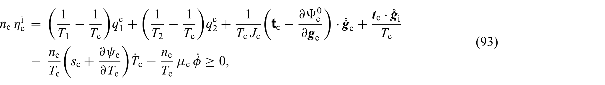
Next we examine the case that there is a common contact interface ${\mathcal{S}}_1\approx {\mathcal{S}}_2={\mathcal{S}}_{\mathrm{c}}$ . Inserting (73) and (80) into the second part of (74) and using the second part of (86), we find

$$\begin{array}{c}{n}_{\mathrm{c}}{\eta }_{\mathrm{c}}^{\mathrm{i}}=(\frac{1}{T_1}-\frac{1}{T_{\mathrm{c}}})q_1^{\mathrm{c}}+(\frac{1}{T_2}-\frac{1}{T_{\mathrm{c}}})q_2^{\mathrm{c}}+\frac{{\mathit{t}}_{\mathrm{c}}·({\mathit{v}}_2-{\mathit{v}}_1)}{T_{\mathrm{c}}}-\frac{n_{\mathrm{c}}}{T_{\mathrm{c}}}({\stackrel{·}{\psi }}_{\mathrm{c}}+{\stackrel{·}{T}}_{\mathrm{c}}{s}_{\mathrm{c}})\ge 0.\hfill \end{array}$$

(92)

Further inserting (21) and (84), and introducing the nominal contact traction ${\mathsf{t}}_{\mathrm{c}}:=J_{\mathrm{c}}{\mathit{t}}_{\mathrm{c}}$ , we find

$$\begin{array}{c}{n}_{\mathrm{c}}{\eta }_{\mathrm{c}}^{\mathrm{i}}=(\frac{1}{T_1}-\frac{1}{T_{\mathrm{c}}})q_1^{\mathrm{c}}+(\frac{1}{T_2}-\frac{1}{T_{\mathrm{c}}})q_2^{\mathrm{c}}+\frac{1}{T_{\mathrm{c}}{J}_{\mathrm{c}}}({\mathsf{t}}_{\mathrm{c}}-\frac{\partial {\mathrm{\Psi }}_{\mathrm{c}}^0}{\partial {\mathit{g}}_{\mathrm{e}}})·{\stackrel{°}{\mathit{g}}}_{\mathrm{e}}+\frac{{\mathit{t}}_{\mathrm{c}}·{\stackrel{°}{\mathit{g}}}_{\mathrm{i}}}{T_{\mathrm{c}}}\hfill \\ \multicolumn{1}{c}{-\frac{n_{\mathrm{c}}}{T_{\mathrm{c}}}(s_{\mathrm{c}}+\frac{\partial {\psi }_{\mathrm{c}}}{\partial T_{\mathrm{c}}}){\stackrel{·}{T}}_{\mathrm{c}}-\frac{n_{\mathrm{c}}}{T_{\mathrm{c}}}{\mu }_{\mathrm{c}}\stackrel{·}{\varphi }\ge 0,}\end{array}$$

(93)

where ${\mathrm{\Psi }}_{\mathrm{c}}^0:=J_{\mathrm{c}}{n}_{\mathrm{c}}{\psi }_{\mathrm{c}}=N_{\mathrm{c}}{\psi }_{\mathrm{c}}$ and where

$$\begin{array}{c}{\mu }_{\mathrm{c}}:=\frac{\partial {\psi }_{\mathrm{c}}}{\partial \varphi }\hfill \end{array}$$

(94)

denotes the chemical potential associated with the interface reactions. Here, $J_{\mathrm{c}}$ is the reference value for the area stretch, chosen analogously to $n_{\mathrm{c}}$ in (39). As inequality (93) is true for any $T_k$ , ${\stackrel{°}{\mathit{g}}}_{\mathrm{e}}$ , ${\stackrel{°}{\mathit{g}}}_{\mathrm{i}}$ , and $\varphi$ , we find the constitutive relations

$${\mathsf{t}}_{\mathrm{c}}=\frac{\partial {\mathrm{\Psi }}_{\mathrm{c}}^{\mathrm{0}}}{\partial {\mathit{g}}_{\mathrm{e}}},{\mathit{t}}_{\mathrm{c}}\cdot {\stackrel{\circ }{\mathit{g}}}_{\mathrm{i}}\ge 0$$

(95)

for the contact tractions,

$$s_{\mathrm{c}}=-\frac{\partial {\psi }_{\mathrm{c}}}{\partial T_{\mathrm{c}}}$$

(96)

for the interfacial entropy,

$${\mu }_{\mathrm{c}}{R}_{\mathrm{c}}\le 0$$

(97)

for the reaction rate $R_{\mathrm{c}}$ (from (40)), and

$$\begin{array}{c}(\frac{1}{T_1}-\frac{1}{T_{\mathrm{c}}})q_1^{\mathrm{c}}+(\frac{1}{T_2}-\frac{1}{T_{\mathrm{c}}})q_2^{\mathrm{c}}\ge 0,\hfill \end{array}$$

(98)

for the contact heat fluxes. Multiplying by $T_1$ , $T_2$ , and $T_{\mathrm{c}}$ (that are all positive), the last statement can be rewritten into

$$\begin{array}{c}{T}_2(T_{\mathrm{c}}-T_1)q_1^{\mathrm{c}}+T_1(T_{\mathrm{c}}-T_2)q_2^{\mathrm{c}}\ge 0.\hfill \end{array}$$

(99)

As this has to be satisfied for any $q_k^{\mathrm{c}}$ , setting either $q_2^{\mathrm{c}}=0$ or $q_1^{\mathrm{c}}=0$ yields the two separate conditions ( $k=1,2$ )

$$(T_{\mathrm{c}}-T_k)q_k^{\mathrm{c}}\ge 0,$$

(100)

for $q_k^{\mathrm{c}}$ . They are, for example, satisfied for the simple and well-known linear heat transfer law

$$\begin{array}{c}{q}_k^{\mathrm{c}}=h_k(T_{\mathrm{c}}-T_k),\hfill \end{array}$$

(101)

where the constant $h_k\ge 0$ is the heat transfer coefficient between body ${\mathcal{B}}_k$ and the interfacial medium. Introducing the mean influx into ${\mathcal{B}}_k$ ,

$$\begin{array}{c}{q}_{\mathrm{m}}^{\mathrm{c}}:=\frac{q_1^{\mathrm{c}}+q_2^{\mathrm{c}}}{2},\hfill \end{array}$$

(102)

and the transfer flux from ${\mathcal{B}}_2$ to ${\mathcal{B}}_1$ (see Figure 3),

$$\begin{array}{c}{q}_{\mathrm{t}}^{\mathrm{c}}:=\frac{q_1^{\mathrm{c}}-q_2^{\mathrm{c}}}{2},\hfill \end{array}$$

(103)

such that $q_1^{\mathrm{c}}=q_{\mathrm{m}}^{\mathrm{c}}+q_{\mathrm{t}}^{\mathrm{c}}$ and $q_2^{\mathrm{c}}=q_{\mathrm{m}}^{\mathrm{c}}-q_{\mathrm{t}}^{\mathrm{c}}$ , one can also rewrite inequality (99) into

$$\begin{array}{c}((T_1+T_2)T_{\mathrm{c}}-2T_1{T}_2)q_{\mathrm{m}}^{\mathrm{c}}+(T_2-T_1)T_{\mathrm{c}}{q}_{\mathrm{t}}^{\mathrm{c}}\ge 0.\hfill \end{array}$$

(104)

As this also has to be true for $q_{\mathrm{m}}^{\mathrm{c}}=0$ , we find the further condition

$$(T_2-T_1)q_{\mathrm{t}}^{\mathrm{c}}\ge 0,$$

(105)

which is, for example, satisfied by

$$\begin{array}{c}{q}_{\mathrm{t}}^{\mathrm{c}}=h(T_2-T_1),\hfill \end{array}$$

(106)

where the constant $h\ge 0$ is the heat transfer coefficient between bodies ${\mathcal{B}}_1$ and ${\mathcal{B}}_2$ .

From (62) we can further find that the mean influx is given by

$$\begin{array}{c}{q}_{\mathrm{m}}^{\mathrm{c}}=\frac{1}{2}({\mathit{t}}_{\mathrm{c}}·({\mathit{v}}_2-{\mathit{v}}_1)-n_{\mathrm{c}}{\stackrel{·}{u}}_{\mathrm{c}}),\hfill \end{array}$$

(107)

which in view of (21), (79), (84), the first part of (95), and (96) becomes

$$q_{\mathrm{m}}^{\mathrm{c}}=\frac{1}{2}({\mathit{t}}_{\mathrm{c}}\cdot {\stackrel{\circ }{\mathit{g}}}_{\mathrm{i}}-{\mu }_{\mathrm{c}}{R}_{\mathrm{c}}-n_{\mathrm{c}}{\stackrel{·}{s}}_{\mathrm{c}}{T}_{\mathrm{c}}),$$

(108)

i.e., the mean heat influx is caused by mechanical dissipation (from friction), chemical dissipation (from reactions), and entropy changes at the interface. The three terms are composed of the conjugated pairs identified in Table 1. Although the first two terms are always positive (due to the second part of (95) and (97)) and, thus, lead to an influx of heat into the bodies, the third term can be positive or negative. It, thus, allows for a heat flux from the bodies into the interface, where the heat is stored as internal energy, see the example in Section 6.2.2. Defining the contact enthalpy per bonding site $e_{\mathrm{c}}$ from

$$\begin{array}{c}{n}_{\mathrm{c}}{e}_{\mathrm{c}}:=n_{\mathrm{c}}{u}_{\mathrm{c}}-{\mathit{t}}_{\mathrm{c}}·\mathit{g},\hfill \end{array}$$

(109)

which is the logical extension of the classical enthalpy definition, ⁸ one finds

$$\begin{array}{c}{q}_{\mathrm{m}}^{\mathrm{c}}=-\frac{n_{\mathrm{c}}}{2}{\stackrel{·}{e}}_{\mathrm{c}}{|}_{{\mathrm{t}}_{\mathrm{c}}=\mathrm{fixed}},\hfill \end{array}$$

(110)

based on the Lie derivative of (19). Thus, the mean heat influx is proportional to the enthalpy change at constant nominal contact traction. Following the classical definition [85], the contact reactions can thus be classified according to

$$\begin{array}{c}{q}_{\mathrm{m}}^{\mathrm{c}}\{\begin{array}{cc}>0\hfill & \mathrm{exothermic}\mathrm{contact}\mathrm{reaction},\hfill \\ \multicolumn{1}{c}{=0}& \mathrm{isothermic}\mathrm{contact}\mathrm{reaction},\hfill \\ \multicolumn{1}{c}{<0}& \mathrm{endothermic}\mathrm{contact}\mathrm{reaction},\hfill \end{array}\hfill \end{array}$$

(111)

in case there is no heat coming from mechanical dissipation ( ${\mathit{t}}_{\mathrm{c}}·{\stackrel{°}{\mathit{g}}}_{\mathrm{i}}=0$ ). Corresponding examples are given in Section 6.2.

Remark 4.3. Interface equation (108) is analogous to the bulk equation (91). While (91) describes the entropy evolution in each body, (108) describes the entropy evolution of the contact interface. In case of transfer law (101), this evolution law explicitly follows from (102) and (108) as

$$\begin{array}{c}{n}_{\mathrm{c}}{T}_{\mathrm{c}}{\stackrel{·}{s}}_{\mathrm{c}}={\mathit{t}}_{\mathrm{c}}·{\stackrel{°}{\mathit{g}}}_{\mathrm{i}}-{\mu }_{\mathrm{c}}{R}_{\mathrm{c}}-(h_1+h_2)T_{\mathrm{c}}+h_1{T}_1+h_2{T}_2.\hfill \end{array}$$

(112)

Like (91), it can be rewritten as an evolution law for the temperature using the entropy-temperature relationship, i.e. (96). The analogy between (91) and (108) is not complete, as (91) contains an explicit heat source, whereas (108) contains a chemical dissipation term. In principle, an explicit heat source can also be considered on the interface, whereas a chemical reaction can also be considered in the bulk. This would lead to a complete analogy between (108) and (91). In the absence of chemical reactions, (108) resorts to the thermo-mechanical energy balance found in older works, see see [2, 4, 5].

Remark 4.4. A special case is $s_{\mathrm{c}}=0\mathrm{for}\mathrm{all}t$ (for example, because there is no interfacial medium), see the example in Section 6.2.1. In this case ${\stackrel{·}{s}}_{\mathrm{c}}=0$ , such that (108) becomes $2q_{\mathrm{m}}^{\mathrm{c}}={\mathit{t}}_{\mathrm{c}}·{\stackrel{°}{\mathit{g}}}_{\mathrm{i}}-n_{\mathrm{c}}{\mu }_{\mathrm{c}}\stackrel{·}{\varphi }$ , which is not an evolution law for $T_{\mathrm{c}}$ anymore, but just an expression for the energy influx into ${\mathcal{B}}_1$ and ${\mathcal{B}}_2$ .

Remark 4.5. According to (108), equal energy flows from the interface into bodies ${\mathcal{B}}_1$ and ${\mathcal{B}}_2$ . The transfer heat flux $q_t^{\mathrm{c}}$ then accounts for the possibility that the bodies heat up differently. Alternatively, as considered in [13, 16, 18], factors can be proposed for the relative contributions going into the two bodies. The work in [16] also accounts for a loss of the interface heat to other bodies, such as an interfacial gas.

Remark 4.6. The nominal traction ${\mathsf{t}}_{\mathrm{c}}:=J_{\mathrm{c}}{\mathit{t}}_{\mathrm{c}}$ is not a physically attained traction. Only the traction ${\mathit{t}}_{\mathrm{c}}=n_{\mathrm{c}}\partial {\psi }_{\mathrm{c}}/\partial {\mathit{g}}_{\mathrm{e}}$ is. As $n_{\mathrm{c}}\ne n_{\mathrm{c}}({\mathit{g}}_{\mathrm{e}})$ , one can also write ${\mathit{t}}_{\mathrm{c}}=\partial {\mathrm{\Psi }}_{\mathrm{c}}/\partial {\mathit{g}}_{\mathrm{e}}$ , for ${\mathrm{\Psi }}_{\mathrm{c}}:=n_{\mathrm{c}}{\psi }_{\mathrm{c}}$ .

Remark 4.7. Multiplying (108) by the area change $J_{\mathrm{c}}$ yields

$$\begin{array}{c}{\mathsf{q}}_{\mathrm{m}}^{\mathrm{c}}:=J_{\mathrm{c}}{q}_{\mathrm{m}}^{\mathrm{c}}=\frac{1}{2}({\mathsf{t}}_{\mathrm{c}}·{\stackrel{°}{\mathit{g}}}_{\mathrm{i}}-{\mathsf{M}}_{\mathrm{c}}\stackrel{·}{\varphi }-{\stackrel{·}{\mathsf{S}}}_{\mathrm{c}}{T}_{\mathrm{c}}),\hfill \end{array}$$

(113)

where ${\mathsf{S}}_{\mathrm{c}}:=N_{\mathrm{c}}{s}_{\mathrm{c}}$ and ${\mathsf{M}}_{\mathrm{c}}:=N_{\mathrm{c}}{\mu }_{\mathrm{c}}$ are the contact entropy and chemical potential per reference area. Owing to ${\mathrm{\Psi }}_{\mathrm{c}}^0:=N_{\mathrm{c}}{\psi }_{\mathrm{c}}$ , (94), and (96), they follow directly from

$$\begin{array}{c}{\mathsf{S}}_{\mathrm{c}}=-\frac{\partial {\mathrm{\Psi }}_{\mathrm{c}}^0}{\partial T_{\mathrm{c}}},{\mathsf{M}}_{\mathrm{c}}=\frac{\partial {\mathrm{\Psi }}_{\mathrm{c}}^0}{\partial \varphi }.\hfill \end{array}$$

(114)

Remark 4.8. Alternatively to transfer laws for $q_1^{\mathrm{c}}$ and $q_2^{\mathrm{c}}$ , such as (101), one can also propose laws for $q_{\mathrm{t}}^{\mathrm{c}}$ and $q_{\mathrm{m}}^{\mathrm{c}}$ . Examples are given by (106) and

$$\begin{array}{c}{q}_{\mathrm{m}}^{\mathrm{c}}=h_{\mathrm{m}}(T_{\mathrm{c}}-\frac{2T_1{T}_2}{T_1+T_2}),\hfill \end{array}$$

(115)

for some $h_{\mathrm{m}}\ge 0$ , as they satisfy condition (104).

Remark 4.9. In case $q_{\mathrm{m}}^{\mathrm{c}}=0$ and relation (101) holds, $T_{\mathrm{c}}$ explicitly follows from (102) as

$$\begin{array}{c}{T}_{\mathrm{c}}=\frac{h_1{T}_1+h_2{T}_2}{h_1+h_2}.\hfill \end{array}$$

(116)

One can then find the well-known relation $h^{-1}=h_1^{-1}+h_2^{-1}$ from (103) and (106), which also has to be true for $q_{\mathrm{m}}^{\mathrm{c}}\ne 0$ in case all $h_k$ are constants.

Remark 4.10. In case of perfect thermal contact $T_{\mathrm{c}}=T_1=T_2$ , the fluxes $q_1^{\mathrm{c}}$ and $q_2^{\mathrm{c}}$ become the unknown Lagrange multipliers to the thermal contact constraints $T_1=T_{\mathrm{c}}$ and $T_1=T_{\mathrm{c}}$ . Alternatively, $q_{\mathrm{t}}^{\mathrm{c}}$ and $q_{\mathrm{m}}^{\mathrm{c}}$ can be used as the Lagrange multipliers to the constraints $T_2=T_1$ and $T_{\mathrm{c}}=(T_1+T_2)/2$ .

4.4. Constitutive equations for non-touching (non-dissipative) interactions

In case of non-touching (long-range) interactions, the two surfaces remain distinct, i.e., ${\mathcal{S}}_1\ne {\mathcal{S}}_2$ . For simplification we consider that the surfaces have the uniform temperatures $T_1$ and $T_2$ , and that the space between ${\mathcal{S}}_1$ and ${\mathcal{S}}_2$ has no mass, temperature or entropy, i.e., $s_{\mathrm{c}}\equiv 0$ . Further, because the surfaces do not touch, no bonding can take place, i.e., $\varphi \equiv 0$ . The Helmholtz free energy of the interface then is

$$\begin{array}{c}{\psi }_{12}=u_{12},\hfill \end{array}$$

(117)

so that ${\stackrel{·}{u}}_{12}={\stackrel{·}{\psi }}_{12}$ . The Helmholtz free energy is now considered to take the form

$$\begin{array}{c}{\psi }_{12}={\psi }_{12}({\mathit{x}}_1,{\mathit{x}}_2),\hfill \end{array}$$

(118)

such that

$$\begin{array}{c}{\stackrel{·}{\psi }}_{12}=\frac{\partial {\psi }_{12}}{\partial {\mathit{x}}_1}·{\mathit{v}}_1+\frac{\partial {\psi }_{12}}{\partial {\mathit{x}}_2}·{\mathit{v}}_2.\hfill \end{array}$$

(119)

Inserting this into (60) yields

$$\begin{array}{c}{\int }_{{\mathcal{S}}_1}({\mathit{t}}_1^{\mathrm{c}}+n_1\frac{\partial {\psi }_2^{\mathrm{c}}}{\partial {\mathit{x}}_1})·{\mathit{v}}_1\mathrm{d}{a}_1+{\int }_{{\mathcal{S}}_2}({\mathit{t}}_2^{\mathrm{c}}+n_2\frac{\partial {\psi }_1^{\mathrm{c}}}{\partial {\mathit{x}}_2})·{\mathit{v}}_2\mathrm{d}{a}_2+{\int }_{{\mathcal{S}}_1}{q}_1^{\mathrm{c}}\mathrm{d}{a}_1+{\int }_{{\mathcal{S}}_2}{q}_2^{\mathrm{c}}\mathrm{d}{a}_2=0\hfill \end{array}$$

(120)

where

$$\begin{array}{c}{\psi }_1^{\mathrm{c}}:={\int }_{{\mathcal{S}}_1}{n}_1{\psi }_{12}\mathrm{d}{a}_1,{\psi }_2^{\mathrm{c}}:={\int }_{{\mathcal{S}}_2}{n}_2{\psi }_{12}\mathrm{d}{a}_2.\hfill \end{array}$$

(121)

Noting that ${\mathit{v}}_k$ and $q_k^{\mathrm{c}}$ are arbitrary and can be independently taken as zero, we find

$${\mathit{t}}_1^{\mathrm{c}}=-n_1\frac{\partial {\psi }_2^{\mathrm{c}}}{\partial {\mathit{x}}_1},{\mathit{t}}_2^{\mathrm{c}}=-n_2\frac{\partial {\psi }_1^{\mathrm{c}}}{\partial {\mathit{x}}_2},$$

(122)

for the interaction tractions, and

$$\begin{array}{c}{\int }_{{\mathcal{S}}_1}{q}_1^{\mathrm{c}}\mathrm{d}{a}_1+{\int }_{{\mathcal{S}}_2}{q}_2^{\mathrm{c}}\mathrm{d}{a}_2=0,\hfill \end{array}$$

(123)

for the interaction heat fluxes. At the same time (72) and the second part of (74) yield

$$\begin{array}{c}{\int }_{{\mathcal{S}}_1}\frac{q_1^{\mathrm{c}}}{T_1}\mathrm{d}{a}_1+{\int }_{{\mathcal{S}}_2}\frac{q_2^{\mathrm{c}}}{T_2}\mathrm{d}{a}_2\ge 0.\hfill \end{array}$$

(124)

If the temperature is constant, one can multiply this by $T_1{T}_2$ and insert (123) to get

$$(T_2-T_1){\int }_{{\mathcal{S}}_1}{q}_1^{\mathrm{c}}\mathrm{d}{a}_1\ge 0,$$

(125)

which is the corresponding statement to (105) for long-range interactions. The traction laws in (122) are identical to those obtained from a variational principle [31].

5. Constitutive examples for contact

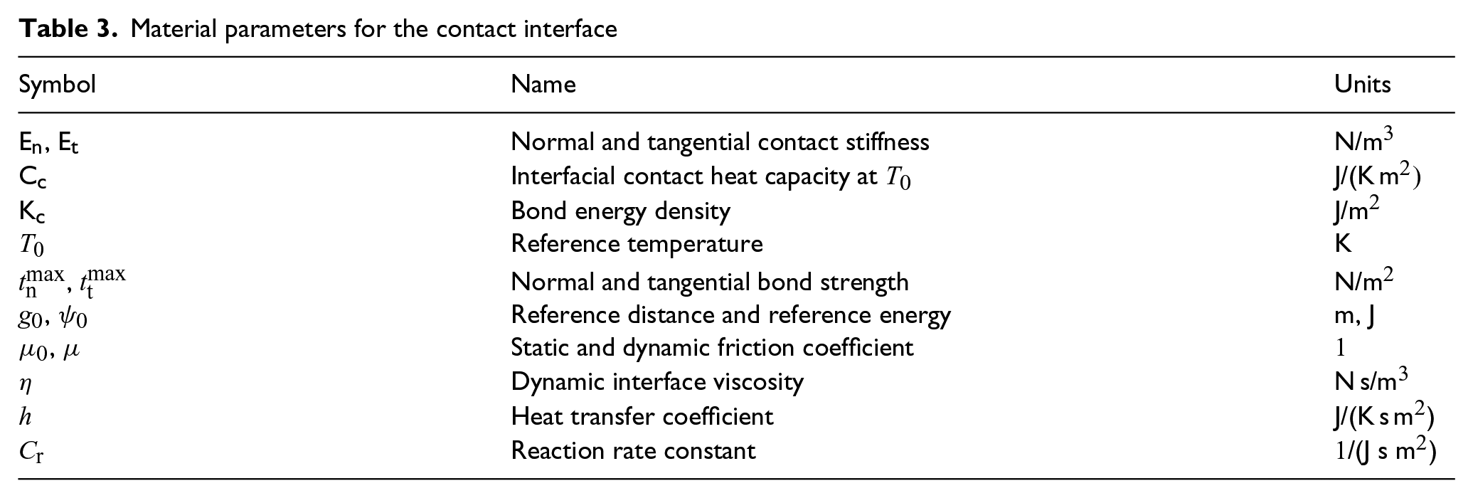
This section lists examples for the preceding constitutive equations for contact and long-range interaction accounting for the coupling between mechanical, thermal, and chemical fields. The examples are based on the material parameters defined in Table 3. Although many of the examples are partially known, their thermo-chemo-mechanical coupling has not yet been explored in detail.

Table 3.

Material parameters for the contact interface

Symbol	Name	Units
${\mathsf{E}}_{\mathsf{n}}$ , ${\mathsf{E}}_{\mathsf{t}}$	Normal and tangential contact stiffness	N/m3
${\mathsf{C}}_{\mathsf{c}}$	Interfacial contact heat capacity at $T_0$	J/(K m2)
${\mathsf{K}}_{\mathsf{c}}$	Bond energy density	J/m2
$T_0$	Reference temperature	K
$t_{\mathrm{n}}^{\max }$ , $t_{\mathrm{t}}^{\max }$	Normal and tangential bond strength	N/m2
$g_0$ , ${\psi }_0$	Reference distance and reference energy	m, J
${\mu }_0$ , $\mu$	Static and dynamic friction coefficient	$1$
$\eta$	Dynamic interface viscosity	N s/m3
$h$	Heat transfer coefficient	J/(K s m2)
$C_{\mathrm{r}}$	Reaction rate constant	$1$ /(J s m2)

5.1. Contact potential

A simple example for the contact potential (per unit reference area) is the quadratic function

$$\begin{array}{c}{\mathrm{\Psi }}_{\mathrm{c}}^0({\mathit{g}}_{\mathrm{e}},T_{\mathrm{c}},\varphi )=\frac{1}{2}{\mathit{g}}_{\mathrm{e}}·{\mathsf{E}}_{\mathrm{c}}{\mathit{g}}_{\mathrm{e}}-\frac{{\mathsf{C}}_{\mathsf{c}}}{2T_0}{(T_{\mathrm{c}}-T_0)}^2+\frac{{\mathsf{K}}_{\mathsf{c}}}{2}{(\varphi -1)}^2,\hfill \end{array}$$

(126)

with ⁹

$$\begin{array}{c}{\mathsf{E}}_{\mathrm{c}}={\mathsf{E}}_{\mathrm{n}}\mathit{n}\otimes \mathit{n}+{\mathsf{E}}_{\mathrm{t}}\mathit{i},\hfill \end{array}$$

(127)

where

$$\begin{array}{c}\mathit{i}:=\mathbf{1}-\mathit{n}\otimes \mathit{n}\hfill \end{array}$$

(128)

is the surface identity on ${\mathcal{S}}_{\mathrm{c}}$ . Here, ${\mathsf{E}}_{\mathsf{n}}$ and ${\mathsf{E}}_{\mathsf{t}}$ denote the normal and tangential contact stiffness (e.g. according to a penalty regularization), ${\mathsf{C}}_{\mathrm{c}}$ denotes the contact heat capacity (at $T_{\mathrm{c}}=T_0$ ) and ${\mathsf{K}}_{\mathrm{c}}$ denotes the bond energy. (126) corresponds to an extension of the models of Johansson and Klarbring [2], Strömberg et al. [5] and Oancea and Laursen [4] to chemical bonding. The parameters ${\mathsf{E}}_{•}$ , ${\mathsf{C}}_{\mathsf{c}}$ and ${\mathsf{K}}_{\mathsf{c}}$ are defined here per undeformed surface area. They can be constant or depend on the other contact state variables, i.e. ${\mathsf{E}}_{•}={\mathsf{E}}_{•}(T_{\mathrm{c}},\varphi )$ , ${\mathsf{C}}_{\mathsf{c}}={\mathsf{C}}_{\mathsf{c}}({\mathit{g}}_{\mathrm{e}},\varphi )$ and ${\mathsf{K}}_{\mathsf{c}}={\mathsf{K}}_{\mathsf{c}}({\mathit{g}}_{\mathrm{e}},T_{\mathrm{c}})$ . If they are constant, (95.1) and (114) yield the contact traction, entropy and chemical potential (per reference area)

$$\begin{array}{c}{\mathsf{t}}_{\mathsf{c}}={\mathsf{E}}_{\mathsf{c}}{\mathit{g}}_{\mathrm{e}},\hfill \\ \multicolumn{1}{c}{{\mathsf{S}}_{\mathsf{c}}={\mathsf{C}}_{\mathsf{c}}(T_{\mathrm{c}}/T_0-1),}\\ \multicolumn{1}{c}{{\mathsf{M}}_{\mathsf{c}}={\mathsf{K}}_{\mathsf{c}}(\varphi -1).}\end{array}$$

(129)

If ${\mathsf{E}}_{•}$ , ${\mathsf{C}}_{\mathsf{c}}$ and ${\mathsf{K}}_{\mathsf{c}}$ are not constant, further terms are generated from (95.1) and (114). An example is given in (162).

Remark 5.1. As noted in Remark 3.4, the first term in (126) is zero if the sticking constraint is enforced exactly. In that case, the elastic gap ${\mathit{g}}_{\mathrm{e}}$ is zero, while ${\mathsf{E}}_{\mathrm{c}}$ approaches infinity. If there is no mass associated with the contact interface, its heat capacity ${\mathsf{C}}_{\mathrm{c}}$ , and hence the second term in (126), is also zero. On the other hand, non-zero ${\mathit{g}}_{\mathrm{e}}$ can be used to capture the deformation of surface asperities during contact (see Remark 2.2), while non-zero ${\mathsf{C}}_{\mathrm{c}}$ can be used to capture the heat capacity of trapped wear debris [2].

Remark 5.2. The last part in (126) corresponds to a classical surface energy. In the unbonded state, ( $\varphi =0$ ) the free surface energy is ${\mathsf{K}}_{\mathrm{c}}/2$ .

Remark 5.3. Choice (126) has minimum energy at full bonding ( $\varphi =1$ ). As $0\le \varphi \le 1$ , ${\mu }_{\mathrm{c}}\le 0$ follows for ${\mathsf{K}}_{\mathrm{c}}>0$ . Thus, $R_{\mathrm{c}}\ge 0$ owing to (97), which leads to $\stackrel{·}{\varphi }\ge 0$ due to (40). Hence, according to (40) and (126), the bonding state $\varphi$ is monotonically increasing over time. Then only mechanical debonding, illustrated by the examples in Sections 5.2 and 6.3, leads to a decrease in $\varphi$ . Chemical debonding, on the other hand, requires a modification of (126), see the following remark.

Remark 5.4. One can change the last term of (126) into

$$\begin{array}{c}\frac{{\mathsf{K}}_{\mathsf{c}}}{2}{(\varphi -{\varphi }_{\mathrm{eq}})}^2,\hfill \end{array}$$

(130)

such that the minimum energy state is at $\varphi ={\varphi }_{\mathrm{eq}}$ . This case implies that chemical equilibrium is a balance of bonding and debonding reactions, as in the model of [47]. An example for this is given in Section 5.7. Like ${\mathsf{K}}_{\mathsf{c}}$ , the parameter $0\le {\varphi }_{\mathrm{eq}}\le 1$ can be a function of ${\mathit{g}}_{\mathrm{e}}$ and $T_{\mathrm{c}}$ .

Remark 5.5. The contact traction ${\mathit{t}}_{\mathrm{c}}={\mathsf{t}}_{\mathrm{c}}/J_{\mathrm{c}}$ can be decomposed into the contact pressure $p_{\mathrm{c}}=-\mathit{n}·{\mathit{t}}_{\mathrm{c}}$ and tangential contact traction ${\mathit{t}}_{\mathrm{t}}=\mathit{i}{\mathit{t}}_{\mathrm{c}}$ (such that ${\mathit{t}}_{\mathrm{c}}=-p_{\mathrm{c}}\mathit{n}+{\mathit{t}}_{\mathrm{t}}$ ). From (127)–(129.1) and ${\epsilon }_{•}:={\mathsf{E}}_{•}/J_{\mathrm{c}}$ thus follow $p_{\mathrm{c}}=-{\epsilon }_{\mathrm{n}}{g}_{\mathrm{n}}$ and ${\mathit{t}}_{\mathrm{t}}={\epsilon }_{\mathrm{t}}{\mathit{g}}_{\mathrm{et}}$ , where $g_{\mathrm{n}}$ and ${\mathit{g}}_{\mathrm{et}}$ are the normal and tangential parts of ${\mathit{g}}_{\mathrm{e}}$ following from (15).

Remark 5.6 The normal contact contribution in (126) and (129.1) is only active up to a debonding limit. Beyond that it becomes inactive, i.e., by setting ${\mathsf{E}}_{\mathrm{n}}=0$ . This is discussed in the following section.

5.2. Adhesion/debonding limit

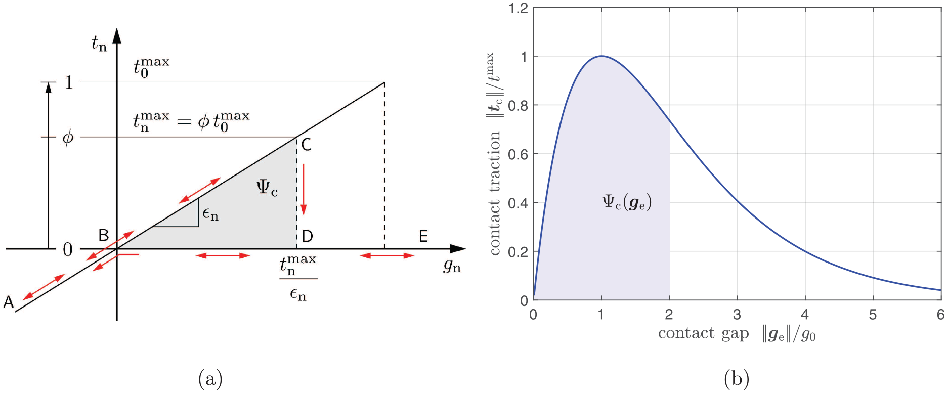
An adhesion or debonding limit implies a lower bound on the contact pressure $p_{\mathrm{c}}$ , i.e.,

$$\begin{array}{c}-p_{\mathrm{c}}\le t_{\mathrm{n}}^{\max },\hfill \end{array}$$

(131)

where the tensile limit (or bond strength) $t_{\mathrm{n}}^{\max }$ can depend on the contact state, i.e., $t_{\mathrm{n}}^{\max }=t_{\mathrm{n}}^{\max }(T_{\mathrm{c}},\varphi )$ . An example is

$$\begin{array}{c}{t}_{\mathrm{n}}^{\max }=\varphi \frac{T_0}{T_{\mathrm{c}}}{t}_0^{\max }.\hfill \end{array}$$

(132)

According to this, the bond strength is increasing with $\varphi$ and decreasing with $T_{\mathrm{c}}$ .

Once the limit is reached, sudden debonding occurs, resulting in $\varphi =0$ . ¹⁰ This makes debonding (mechanically) irreversible (unless $t_{\mathrm{n}}^{\max }=0$ ). Figure 5(a) shows a graphical representation of this.

Figure 5.

Normal contact behavior: (a) irreversible debonding according to (129.1) and (131); (b) reversible adhesion according to (133), adapted from [86].

Debonding can also be described in the context of CZMs. An example is the exponential CZM

$$\begin{array}{c}{\mathrm{\Psi }}_{\mathrm{c}}=-t^{\max }(g_{\mathrm{e}}+g_0)\exp (1-\frac{g_{\mathrm{e}}}{g_0}),g_{\mathrm{e}}:=\parallel {\mathit{g}}_{\mathrm{e}}\parallel ,\hfill \end{array}$$

(133)

where $t^{\max }$ and $g_0$ are material parameters that can depend on $T_{\mathrm{c}}$ and $\varphi$ . Equation (133) is an adaption of the model of Xu and Needleman [39]. It leads to the contact traction

$$\begin{array}{c}{\mathit{t}}_{\mathrm{c}}=-t^{\max }\exp (1-\frac{g_{\mathrm{e}}}{g_0})\frac{{\mathit{g}}_{\mathrm{e}}}{g_0},\hfill \end{array}$$

(134)

according to the first part of (95) and Remark 4.6. Equation (134) replaces the traction law in the first part of (129) and its limit (131). It is illustrated in Figure 5(b). Traction law (134) is reversible unless $t^{\max }$ is a function of $\varphi$ that drops to zero beyond some $g_{\mathrm{e}}$ .

Model (133) is similar to adhesion models for non-touching contact discussed next.

5.3. Non-touching adhesion

An example for non-touching contact interactions according to Section 4.4 is the interaction potential

$$\begin{array}{c}{\psi }_{12}({\overline{g}}_k)={\psi }_0[\frac{1}{45}{\left(\frac{g_0}{{\overline{g}}_k}\right)}^{10}-\frac{1}{3}{\left(\frac{g_0}{{\overline{g}}_k}\right)}^4],{\overline{g}}_k:=\parallel {\mathit{x}}_k-{\mathit{x}}_{\ell }\parallel >0,\hfill \end{array}$$

(135)

where ${\psi }_0$ and $g_0$ are constants and where either $k=1$ and $\ell =2$ or $k=2$ and $\ell =1$ . From (121) and (122) then follows

$$\begin{array}{c}{\mathit{t}}_k^{\mathrm{c}}({\mathit{x}}_k)=-n_k{\int }_{{\mathcal{S}}_{\ell }}{n}_{\ell }\frac{\partial {\psi }_{12}}{\partial {\mathit{x}}_k}\mathrm{d}{a}_{\ell },\hfill \end{array}$$

(136)

with

$$\begin{array}{c}-\frac{\partial {\psi }_{12}}{\partial {\mathit{x}}_k}=\frac{{\psi }_0}{g_0}[\frac{10}{45}{\left(\frac{g_0}{{\overline{g}}_k}\right)}^{11}-\frac{4}{3}{\left(\frac{g_0}{{\overline{g}}_k}\right)}^5]{\overline{\mathit{g}}}_k,{\overline{\mathit{g}}}_k:=\frac{{\mathit{x}}_k-{\mathit{x}}_{\ell }}{{\overline{g}}_k}.\hfill \end{array}$$

(137)

These expressions are valid for general surface geometries and arbitrarily long-range interactions. For short-range interactions between locally flat surfaces, these expressions can be integrated analytically to give [31]

$$\begin{array}{c}{\mathit{t}}_k^{\mathrm{c}}({\mathit{x}}_k)=2\pi n_1{n}_2{g}_{\mathrm{n}}{\psi }_{12}(g_{\mathrm{n}}){\mathit{n}}_{\mathrm{p}},\hfill \end{array}$$

(138)

where $g_{\mathrm{n}}$ is the normal gap between point ${\mathit{x}}_k$ and surface ${\mathcal{S}}_{\ell }$ , and ${\mathit{n}}_{\mathrm{p}}$ is the surface normal of ${\mathcal{S}}_{\ell }$ at ${\mathit{x}}_{\mathrm{p}}$ .

Remark 5.7. The surface interaction potential (135) can be derived from the classical Lennard–Jones potential for volume interactions [29, 87].

Remark 5.8. Example (135) is only valid for separated bodies ( ${\overline{g}}_k>0$ ). Formulation (136) can however also be used for other potentials ${\psi }_{12}$ that admit penetrating bodies (with negative distances). Examples, such as a penalty-type contact formulation, are given in [31]. Computationally, (136) leads to the so-called two-half-pass contact algorithm, which is thus a thermodynamically consistent algorithm.

Remark 5.9. Eq. (136) also applies to the Coulomb potential for electrostatic interactions [31]. However, in order to account for the full electro-mechanical coupling, the present theory needs to be extended.

Remark 5.10. We note again that for non-touching contact, the tractions ${\mathit{t}}_1^{\mathrm{c}}$ and ${\mathit{t}}_2^{\mathrm{c}}$ generally only satisfy global contact equilibrium (46), but not local contact equilibrium (47).

Remark 5.11. Equation (138) is a pure normal contact model that does not produce local tangential contact forces. Tangential contact forces only arise globally when ${\mathit{t}}_k^{\mathrm{c}}$ acts on rough surfaces.

5.4. Sticking limit

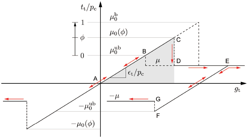
Similar to the debonding limit (131), a sticking limit implies a bound on the tangential traction ${\mathit{t}}_{\mathrm{t}}$ , i.e.,

$$\begin{array}{c}\parallel {\mathit{t}}_{\mathrm{t}}\parallel \le t_{\mathrm{t}}^{\max },\hfill \end{array}$$

(139)

where the limit value $t_{\mathrm{t}}^{\max }$ is generally a function of contact pressure, temperature, and bonding state, i.e., $t_{\mathrm{t}}^{\max }=t_{\mathrm{t}}^{\max }(p_{\mathrm{c}},T_{\mathrm{c}},\varphi )$ . It is reasonable to assume that it is monotonically increasing with $p_{\mathrm{c}}$ and $\varphi$ and decreasing with $T_{\mathrm{c}}$ , e.g.,

$$\begin{array}{c}{t}_{\mathrm{t}}^{\max }={\mu }_0{p}_{\mathrm{c}},\hfill \end{array}$$

(140)

where

$$\begin{array}{c}{\mu }_0=(\varphi {\mu }_0^{\mathrm{b}}+(1-\varphi ){\mu }_0^{\mathrm{ub}})\frac{T_0}{T_{\mathrm{c}}}\hfill \end{array}$$

(141)

is a temperature- and bonding state-dependent coefficient of sticking friction based on the constants ${\mu }_0^{\mathrm{b}}$ and ${\mu }_0^{\mathrm{ub}}$ describing the limits for full bonding and full unbonding, respectively. Once the limit is reached, the bonds break ( $\varphi =0$ ) and tangential sliding occurs, as is discussed in the following section. Figure 6 shows a graphical representation of this.

Figure 6.

Tangential contact behavior: sticking, debonding, and sliding according to (139)–(141) and (143). The latter two are irreversible.

5.5. Sliding models

The simplest viscous friction model satisfying (95.2) is the tangential traction model

$$\begin{array}{c}{\mathit{t}}_{\mathrm{t}}=\frac{{\stackrel{°}{\mathit{g}}}_{\mathrm{i}}}{g_{\mathrm{n}}},\hfill \end{array}$$

(142)

where $\mathit{\eta }$ is the positive-definite dynamic viscosity tensor and $g_{\mathrm{n}}$ is the normal gap. In the isotropic case, $\mathit{\eta }=\eta \mathbf{1}$ .

One of the simplest dry friction models satisfying (95.2) for $p_{\mathrm{c}}\ge 0$ is the Amontons–Coulomb law ¹¹

$$\begin{array}{c}{\mathit{t}}_{\mathrm{t}}=\mathit{\mu }{p}_{\mathrm{c}}\frac{{\stackrel{°}{\mathit{g}}}_{\mathrm{i}}}{\parallel {\stackrel{°}{\mathit{g}}}_{\mathrm{i}}\parallel },\hfill \end{array}$$

(143)

where $\mathit{\mu }$ is the positive-definite coefficient tensor for sliding friction. In the isotropic case, $\mathit{\mu }=\mu \mathbf{1}$ . For adhesion, where $p_{\mathrm{c}}\ge -t_{\mathrm{n}}^{\max }$ , this extends to

$$\begin{array}{c}{\mathit{t}}_{\mathrm{t}}=\mathit{\mu }(p_{\mathrm{c}}+t_{\mathrm{n}}^{\max })\frac{{\stackrel{°}{\mathit{g}}}_{\mathrm{i}}}{\parallel {\stackrel{°}{\mathit{g}}}_{\mathrm{i}}\parallel }.\hfill \end{array}$$

(144)

In the adhesion literature this extension is often attributed to Derjaguin [88], whereas in soil mechanics it is usually referred to as Mohr–Coulomb’s law. Note that $\mathit{\mu }{t}_{\mathrm{n}}^{\max }$ can be taken as a new constant. The application of (144) to coupled adhesion and friction in the context of nonlinear 3D elasticity has been recently considered by Mergel et al. [32, 89].

Remark 5.12. A transition model between dry (rate-independent) and viscous (rate-dependent) sliding friction is Stribeck’s curve, see, e.g., [90].

Remark 5.13. The above sliding models can be temperature dependent. An example for a temperature-dependent friction coefficient $\mu =\mu (T_{\mathrm{c}})$ is given in [67]. Temperature-dependent viscosity models are e.g. discussed in [91] and [92].

Remark 5.14. The present formulation assumes fixed bonding sites that break during sliding friction. Sliding friction is, thus, independent from $\varphi$ . Bonding sites can, however, also be mobile and, hence, remain intact during sliding. Sliding friction may, thus, depend on $\varphi$ . This requires a mobility model for the bonds, e.g., following the work of [77].

Remark 5.15. The friction coefficient can be considered dependent on the surface deformation, as has been done by [93].

Remark 5.16. Friction coefficients that are dependent on the sliding velocity and (wear) state have been considered in the framework of rate and state friction models [63, 65]. Those models are usually based on an additive decomposition of the shear traction ${\mathit{t}}_{\mathrm{t}}$ instead of an additive slip decomposition as is used here.

Remark 5.17. Note that ${\mathit{t}}_{\mathrm{t}}$ causes the mechanical dissipation ${\mathcal{D}}_{\mathrm{mech}}={\mathit{t}}_{\mathrm{t}}·{\stackrel{°}{\mathit{g}}}_{\mathrm{i}}$ that leads to heating of the contact bodies due to (108). The mechanical dissipation is ${\mathcal{D}}_{\mathrm{mech}}={\stackrel{°}{\mathit{g}}}_{\mathrm{i}}·$ ${\stackrel{°}{\mathit{g}}}_{\mathrm{i}}/g_{\mathrm{n}}$ for model (142) and ${\mathcal{D}}_{\mathrm{mech}}=p_{\mathrm{c}}{\stackrel{°}{\mathit{g}}}_{\mathrm{i}}·\mathit{\mu }{\stackrel{°}{\mathit{g}}}_{\mathrm{i}}/\parallel {\stackrel{°}{\mathit{g}}}_{\mathrm{i}}\parallel$ for model (143); see Section 6.1 for an example.

5.6. Heat transfer

The simplest heat transfer model satisfying condition (105) is the linear relationship already given in (106), where $h>0$ is the heat transfer coefficient, also referred to as the thermal contact conductance. Equation (106) is analogous to the mechanical flux model in (129.1). Similar to the mechanical case, $h\to \infty$ implies $T_2-T_1\to 0$ . In general, $h$ can be a function of the contact pressure, gap, or bonding state, i.e., $h=h(p_{\mathrm{c}},g_{\mathrm{n}},\varphi )$ . Various models have been considered in the past. Those usually consider $h$ to be additively split into a contribution coming from actual contact and contributions coming from radiation and convection across a small contact gap.

During actual contact ( $g_{\mathrm{n}}=0$ , $p_{\mathrm{c}}>0$ ) a simple model is the power law dependency on the contact pressure,

$$\begin{array}{c}h=h_0+h_{\mathrm{c}}{\left(\frac{p_{\mathrm{c}}}{H}\right)}^q,\hfill \end{array}$$

(145)

where $h_0$ , $h_{\mathrm{c}}$ , $H$ , and $q$ are positive constants [3, 94].

This model is a simplification of the more detailed model of Song and Yovanovich [95] that accounts for microscopic contact roughness. Another model for $h$ is the model by Mikic [96]. A new model has also been proposed recently by Martins et al. [97]. The dependency of (145) on the bonding state can, for example, be taken as

$$\begin{array}{c}{h}_0=\varphi h_0^{\mathrm{b}}+(1-\varphi )h_0^{\mathrm{ub}},\hfill \\ \multicolumn{1}{c}{h_{\mathrm{c}}=\varphi h_{\mathrm{c}}^{\mathrm{b}}+(1-\varphi )h_{\mathrm{c}}^{\mathrm{ub}},}\end{array}$$

(146)

i.e., assuming that $h_0$ and $h_{\mathrm{c}}$ increase monotonically with $\varphi$ . Here $h_0^{\mathrm{b}}$ , $h_0^{\mathrm{ub}}$ , $h_{\mathrm{c}}^{\mathrm{b}}$ , and $h_{\mathrm{c}}^{\mathrm{ub}}$ are model constants.

Out of contact ( $g_{\mathrm{n}}>0$ , $p_{\mathrm{c}}=0$ , $\varphi =0$ ), the heat transfer depends on the contact gap. Considering small $g_{\mathrm{n}}$ , Laschet et al. [94] propose an exponential decay of $h$ with $g_{\mathrm{n}}$ was proposed according to

$$\begin{array}{c}h=h_{\mathrm{rad}}+h_{\mathrm{gas}}+(h_0-h_{\mathrm{rad}}-h_{\mathrm{gas}})\exp (-C_{\mathrm{trans}}{g}_{\mathrm{n}}),\hfill \end{array}$$

(147)

where

$$\begin{array}{c}{h}_{\mathrm{rad}}=\frac{c_{\mathrm{rad}}(T_1^2+T_2^2)(T_1+T_2)}{{\epsilon }_1^{-1}+{\epsilon }_2^{-1}-1}\hfill \end{array}$$

(148)

and

$$\begin{array}{c}{h}_{\mathrm{gas}}=\frac{k_{\mathrm{gas}}(T_{\mathrm{c}})}{g_{\mathrm{n}}+g_0(T_{\mathrm{c}})}\hfill \end{array}$$

(149)

correspond to the heat transfer across the gap due to radiation and gas convection, respectively. Here, $C_{\mathrm{trans}}$ , $c_{\mathrm{rad}}$ , ${\epsilon }_1$ , and ${\epsilon }_2$ are constants, while $k_{\mathrm{gas}}$ and $g_0$ depend on the contact temperature $T_{\mathrm{c}}$ .

We note that all the above models are consistent with the second law as long as $h>0$ .

5.7. Bonding reactions

The simplest reaction rate model satisfying condition (97) is the linear relationship,

$$\begin{array}{c}{R}_{\mathrm{c}}=-C_{\mathrm{r}}{\mu }_{\mathrm{c}},\hfill \end{array}$$

(150)

where the constant $C_{\mathrm{r}}\ge 0$ can, for example, be a function of the contact temperature and pressure, i.e., $C_{\mathrm{r}}=C_{\mathrm{r}}(p_{\mathrm{c}},T_{\mathrm{c}})$ . Writing $C_{\mathrm{r}}=n_{\mathrm{c}}{c}_{\mathrm{r}}$ , the reaction equation in (40) thus becomes $\stackrel{·}{\varphi }=-c_{\mathrm{r}}{\mu }_{\mathrm{c}}$ . Alternatively (and in consistency with (97)), $c_{\mathrm{r}}\ge 0$ can be taken as a constant.

Another, more sophisticated example that satisfies (97) is the exponential relationship [75],

$$\begin{array}{c}{R}_{\mathrm{c}}=C_{\mathrm{r}}R{T}_{\mathrm{c}}(1-\exp \frac{{\mu }_{\mathrm{c}}}{R{T}_{\mathrm{c}}}),\hfill \end{array}$$

(151)

where $R$ is the universal gas constant.

Remark 5.18. Plugging the example (129.3) and (39) into (150) yields $R_{\mathrm{c}}=c_{\mathrm{r}}{k}_{\mathrm{c}}(n_{\mathrm{c}}-n_{\mathrm{b}})$ with $k_{\mathrm{c}}={\mathsf{K}}_{\mathrm{c}}/N_{\mathrm{c}}$ , which is a pure forward reaction (see also Remark 5.3). Then $\overleftarrow{k}:=c_{\mathrm{r}}{k}_{\mathrm{c}}$ is the forward reaction rate coefficient. An example on how this could depend on the contact gap is given in [55].

Remark 5.19. On the other hand, modification (130) leads to ${\mathsf{M}}_{\mathrm{c}}={\mathsf{K}}_{\mathrm{c}}(\varphi -{\varphi }_{\mathrm{eq}})$ instead of (129.3). Substituting ${\mathsf{K}}_{\mathrm{c}}=\overrightarrow{{\mathsf{K}}_{\mathrm{c}}}+\overleftarrow{{\mathsf{K}}_{\mathrm{c}}}$ and ${\varphi }_{\mathrm{eq}}=\overrightarrow{{\mathsf{K}}_{\mathrm{c}}}/{\mathsf{K}}_{\mathrm{c}}$ then leads to

$$\begin{array}{c}{\mathsf{M}}_{\mathrm{c}}=\overrightarrow{{\mathsf{K}}_{\mathrm{c}}}(\varphi -1)+\overleftarrow{{\mathsf{K}}_{\mathrm{c}}}\varphi ,\hfill \end{array}$$

(152)

such that (150) leads to (34) with the reaction rates

$$\begin{array}{c}\overrightarrow{R_{\mathrm{c}}}=\overrightarrow{k}(n_{\mathrm{c}}-n_{\mathrm{b}}),\overrightarrow{k}:=c_{\mathrm{r}}\overrightarrow{{\mathsf{K}}_{\mathrm{c}}}/N_{\mathrm{c}},\hfill \\ \multicolumn{1}{c}{\overleftarrow{R_{\mathrm{c}}}=\overleftarrow{k}{n}_{\mathrm{b}},\overleftarrow{k}:=c_{\mathrm{r}}\overleftarrow{{\mathsf{K}}_{\mathrm{c}}}/N_{\mathrm{c}},}\end{array}$$

(153)

for chemical bonding (forward reaction) and debonding (backward reaction), respectively. The case in Remark 5.18 is recovered for the backward reaction rate coefficient $\overrightarrow{k}=0$ .

6. Elementary contact test cases

This section presents the analytical solution of three new elementary contact test cases: thermo-mechanical sliding, thermo-chemical bonding, and thermo-chemo-mechanical debonding. Such test cases are useful, for example, for the verification of a computational implementation. Another test case for thermo-mechanical normal contact can be found in Wriggers and Miehe [3]. All test cases consider two blocks with initial height $H_1$ and $H_2$ brought into contact. The energy and temperature change in the contacting bodies is then computed assuming instantaneous heat transfer through the bodies ( ${\mathit{q}}_k=\mathit{0}$ ), no heat source in the bulk ( ${\overline{r}}_k=0$ ), no boundary heat flux apart from $q_{\mathrm{m}}^{\mathrm{c}}$ ( ${\overline{q}}_k=0$ & $q_{\mathrm{t}}^{\mathrm{c}}=0$ ), equal temperature within the bodies ( $T_1=T_2=T_{\mathrm{c}}$ ), quasi-static deformation ( ${\mathit{D}}_k=\mathit{0}$ ), homogeneous deformation ( ${\mathit{E}}_k\ne {\mathit{E}}_k({\mathit{x}}_k)$ ), uniform contact conditions ( $\mathit{g}\ne \mathit{g}({\mathit{x}}_{\mathrm{c}})$ ), and fixed contact area ( $J_{\mathrm{sk}}=1$ ), such that one can work with the Helmholtz free contact energy ${\mathrm{\Psi }}_{\mathrm{c}}=n_{\mathrm{c}}{\psi }_{\mathrm{c}}$ . ¹² Under these conditions the temperature change within each body is governed by the energy balance

$$\begin{array}{c}{\rho }_{k0}{H}_k{\stackrel{·}{u}}_k=q_{\mathrm{m}}^{\mathrm{c}},\hfill \end{array}$$

(154)

that follows directly from integrating (59) over the reference volume, writing $\mathrm{d}{V}_k=H_k\mathrm{d}{A}_k$ on the left-hand side and applying the divergence theorem on the right. Considering the bulk energy

$$\begin{array}{c}{\psi }_k={\psi }_{\mathrm{mech}}-\frac{c_k}{2T_0}{(T_k-T_0)}^2,\hfill \end{array}$$

(155)

where $c_k$ is the heat capacity per unit mass, leads to

$$\begin{array}{c}{u}_k=u_{\mathrm{mech}}+\frac{c_k}{2T_0}(T_k^2-T_0^2),\hfill \end{array}$$

(156)

due to (75) and (90). For quasi-static deformations then follows ${\stackrel{·}{u}}_k=c_k{T}_k{\stackrel{·}{T}}_k/T_0$ . Inserting this into (154) then gives

$$\begin{array}{c}\frac{C_k}{T_0}{T}_{\mathrm{c}}{\stackrel{·}{T}}_{\mathrm{c}}=q_{\mathrm{m}}^{\mathrm{c}},\hfill \end{array}$$

(157)

where $C_k:=H_k{\rho }_{k0}{c}_k$ is the heat capacity per unit contact area satisfying $C_1=C_2$ .

6.1. Sliding thermodynamics

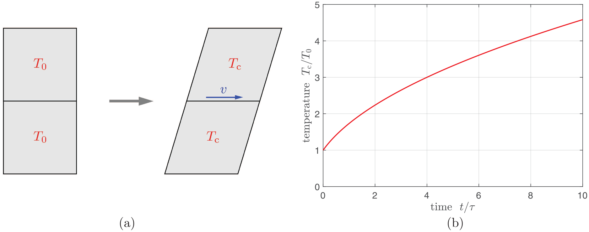
The first test case illustrates thermo-mechanical coupling by calculating the temperature rise due to mechanical sliding. The test case is illustrated in Figure 7(a): two blocks initially at mechanical rest and temperature $T_0$ are subjected to steady sliding with the relative sliding velocity magnitude $v:=\parallel {\stackrel{°}{\mathit{g}}}_{\mathrm{i}}\parallel$ .

Figure 7.

Sliding thermodynamics: (a) model problem; (b) temperature rise during sliding.

Following Störmberg et al. [5] and Oancea and Laursen [4], the contact energy

$$\begin{array}{c}{\mathrm{\Psi }}_{\mathrm{c}}=\frac{1}{2}{\mathit{g}}_{\mathrm{e}}·\mathit{ϵ}{\mathit{g}}_{\mathrm{e}}-\frac{C_{\mathrm{c}}}{2T_0}{(T_{\mathrm{c}}-T_0)}^2\hfill \end{array}$$

(158)

is used with constant $\mathit{ϵ}$ and $C_{\mathrm{c}}$ . Equation (158) leads to the entropy given in (129.2). The mean influx, given by (108) and (113), then becomes

$$\begin{array}{c}2q_{\mathrm{c}}^{\mathrm{m}}={\mathcal{D}}_{\mathrm{mech}}-\frac{C_{\mathrm{c}}}{T_0}{T}_{\mathrm{c}}{\stackrel{·}{T}}_{\mathrm{c}},\hfill \end{array}$$

(159)

where ${\mathcal{D}}_{\mathrm{mech}}=\eta v^2/g_{\mathrm{n}}$ , according to model (142) and ${\mathcal{D}}_{\mathrm{mech}}=\mu \mathrm{pv}$ according to model (143). During stationary sliding ( $v=\mathrm{constant}$ ) the mechanical deformation is time-independent. From (157) thus follows

$$\begin{array}{c}{T}_{\mathrm{c}}{\stackrel{·}{T}}_{\mathrm{c}}=\frac{T_0^2}{\tau },\mathrm{with}\tau :=\frac{C_1+C_2+C_{\mathrm{c}}}{{\mathcal{D}}_{\mathrm{mech}}}{T}_0,\hfill \end{array}$$

(160)

where $\tau$ is the time scale of the temperature rise. Integrating this from the initial condition $T_{\mathrm{c}}(0)=T_0$ leads to the temperature rise

$$\begin{array}{c}{T}_{\mathrm{c}}(t)=T_0\sqrt{1+2t/\tau },\hfill \end{array}$$

(161)

which is shown in Figure 7(b).

6.2. Bonding thermodynamics

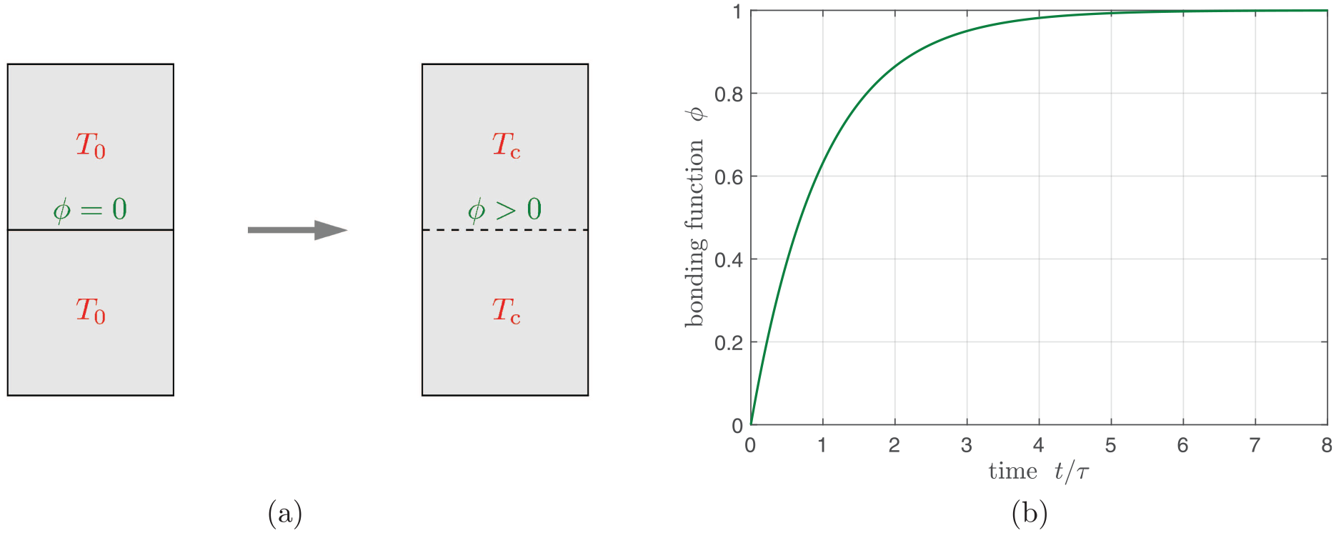
The second test case illustrates thermo-chemical coupling by calculating the temperature change due to chemical bonding. The test case is illustrated in Figure 8(a): two blocks initially unbonded and at temperature $T_0$ are bonding and changing temperature.

Figure 8.

Bonding thermodynamics: (a) model problem; (b) bonding function $\varphi (t)$ .

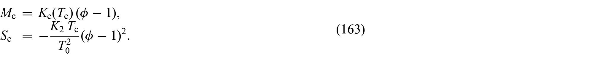
Now, the contact energy

$$\begin{array}{c}{\mathrm{\Psi }}_{\mathrm{c}}=\frac{K_{\mathrm{c}}(T_{\mathrm{c}})}{2}{(\varphi -1)}^2,\mathrm{with}{K}_{\mathrm{c}}(T_{\mathrm{c}})=K_0+K_2\frac{T_{\mathrm{c}}^2}{T_0^2},\hfill \end{array}$$

(162)

is used, which, owing to (114), leads to the chemical potential and entropy

$$\begin{array}{c}{M}_{\mathrm{c}}=K_{\mathrm{c}}(T_{\mathrm{c}})(\varphi -1),\hfill \\ \multicolumn{1}{c}{S_{\mathrm{c}}=-\frac{K_2{T}_{\mathrm{c}}}{T_0^2}{(\varphi -1)}^2.}\end{array}$$

(163)

This, in turn, leads to the internal energy

$$\begin{array}{c}{U}_{\mathrm{c}}=\frac{1}{2}{(\varphi -1)}^2(K_0-K_2\frac{T_{\mathrm{c}}^2}{T_0^2}),\hfill \end{array}$$

(164)

and the bonding ODE

$$\begin{array}{c}\stackrel{·}{\varphi }=\frac{1}{\tau }(1-\varphi ),\mathrm{with}\tau =\frac{n_{\mathrm{c}}}{c_{\mathrm{r}}(T_{\mathrm{c}})K_{\mathrm{c}}(T_{\mathrm{c}})},\hfill \end{array}$$

(165)

according to (40), (78) and (150). ODE (165) can only be solved with knowledge about $T_{\mathrm{c}}=T_{\mathrm{c}}(t)$ .

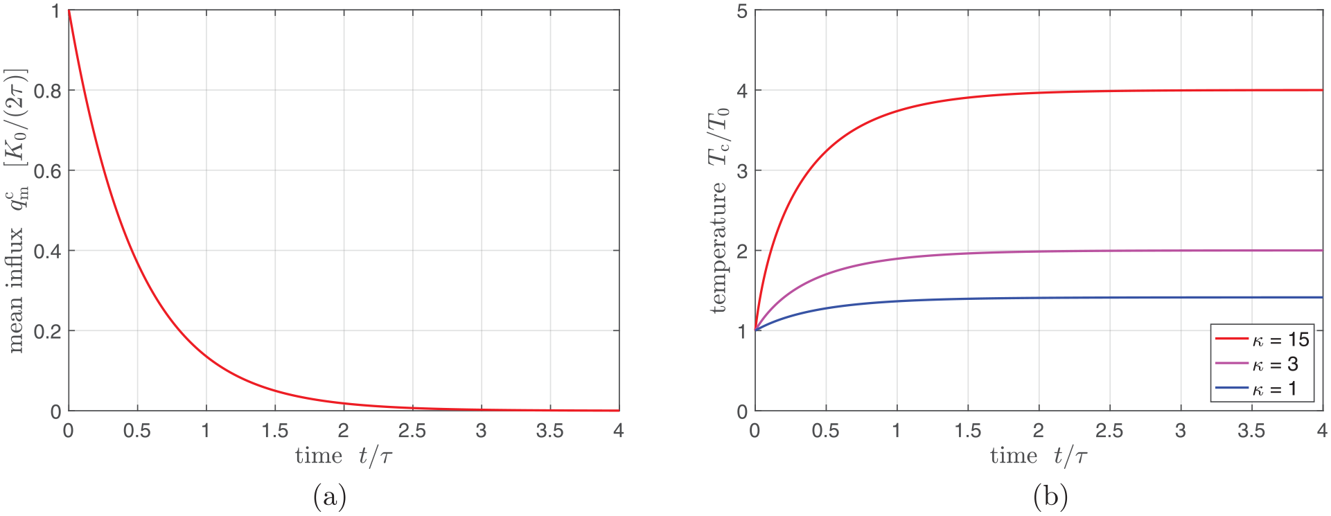
6.2.1. Exothermic bonding

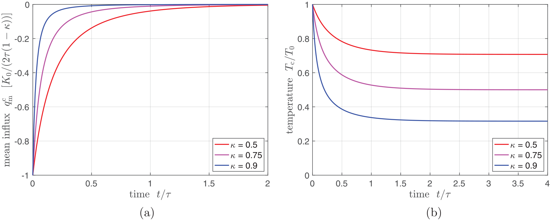
Exothermic bonding occurs for $K_2=0$ (which implies $U_{\mathrm{c}}={\mathrm{\Psi }}_{\mathrm{c}}$ ). Considering $c_{\mathrm{r}}=\mathrm{constant}$ , the bonding ODE becomes independent of $T_{\mathrm{c}}$ and can be integrated from the initial condition $\varphi (0)=0$ to give

$$\begin{array}{c}\varphi (t)=1-e^{-t/\tau },\hfill \end{array}$$

(166)

where $\tau =n_1/(c_{\mathrm{r}}{K}_0)$ is the time scale of the exothermic bonding reaction. Solution (166) is shown in Figure 8(b) The mean influx, given in (108) and (113), then becomes

$$\begin{array}{c}{q}_{\mathrm{m}}^{\mathrm{c}}=\frac{K_0}{2\tau }{e}^{-2t/\tau }.\hfill \end{array}$$

(167)

It satisfies the exothermic condition $q_{\mathrm{m}}^{\mathrm{c}}>0$ and is shown in Figure 9(a). From (157) thus follows

$$\begin{array}{c}{C}_k{T}_{\mathrm{c}}{\stackrel{·}{T}}_{\mathrm{c}}=\frac{K_0{T}_0}{2\tau }{e}^{-2t/\tau },\hfill \end{array}$$

(168)

which can be integrated from the initial condition $T_{\mathrm{c}}(0)=T_0$ to give the temperature rise

$$\begin{array}{c}{T}_{\mathrm{c}}(t)=T_0\sqrt{1+\kappa (1-e^{-2t/\tau })},\mathrm{with}\kappa :=\frac{K_0}{2T_0{C}_k},\hfill \end{array}$$

(169)

shown in Figure 9(b) for various values of $\kappa$ .

Figure 9.

Bonding thermodynamics: (a) heat influx $q_{\mathrm{m}}^{\mathrm{c}}(t)$ and (b) temperature rise $T_{\mathrm{c}}(t)$ during exothermic bonding.

6.2.2. Endothermic bonding

Endothermic bonding occurs for $K_0=0$ in the above model (which implies $U_{\mathrm{c}}=-{\mathrm{\Psi }}_{\mathrm{c}}$ according to (162) and (164)). The mean influx, given in (108) and (113), now becomes

$$\begin{array}{c}{q}_{\mathrm{m}}^{\mathrm{c}}=\frac{K_2}{2T_0^2}{(1-\varphi )}^2(T_{\mathrm{c}}{\stackrel{·}{T}}_{\mathrm{c}}-\frac{1}{\tau }{T}_{\mathrm{c}}^2).\hfill \end{array}$$

(170)

In order to solve (165), a temperature-dependent reaction rate is considered in the form $c_{\mathrm{r}}=c_{\mathrm{r}0}{T}_0^2/T_{\mathrm{c}}^2$ with $c_{\mathrm{r}0}=\mathrm{constant}$ . Thus (166) is still the solution of bonding ODE (165). The time scale now becomes $\tau =n_1/(c_{\mathrm{r}0}{K}_2)$ . From (157) now follows

$$\begin{array}{c}\frac{{\stackrel{·}{T}}_{\mathrm{c}}}{T_{\mathrm{c}}}=\frac{1}{\tau }\frac{\kappa e^{-2t/\tau }}{\kappa e^{-2t/\tau }-1},\mathrm{with}\kappa :=\frac{K_2}{2T_0{C}_k}.\hfill \end{array}$$

(171)

Integrating this from the initial condition $T_{\mathrm{c}}(0)=T_0$ gives the temperature drop

$$\begin{array}{c}{T}_{\mathrm{c}}(t)=T_0\sqrt{\frac{1-\kappa }{1-\kappa e^{-2t/\tau }}},\hfill \end{array}$$

(172)

where the parameter $\kappa$ must be smaller than unity for the temperature to remain physical. According to (170), this now leads to

$$\begin{array}{c}{q}_{\mathrm{m}}^{\mathrm{c}}(t)=-\frac{K_2}{2\tau }\frac{1-\kappa }{{(1-\kappa e^{-2t/\tau })}^2}{e}^{-2t/\tau },\hfill \end{array}$$

(173)

and satisfies $q_{\mathrm{m}}^{\mathrm{c}}<0$ . Figure 10 shows the energy outflux and temperature drop of the contact interface for the endothermic case.

Figure 10.

Bonding thermodynamics: (a) heat influx $q_{\mathrm{m}}^{\mathrm{c}}(t)$ and (b) temperature drop $T_{\mathrm{c}}(t)$ during endothermic bonding.

6.3. Debonding thermodynamics

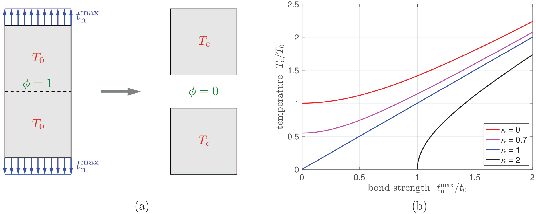
The last test case illustrates thermo-chemo-mechanical coupling by calculating the temperature change due to mechanical debonding. The test case is illustrated in Figure 11(a): two blocks initially bonded and at temperature $T_0$ are pulled apart leading to debonding and rising temperature. Now the contact energy density

$$\begin{array}{c}{\mathrm{\Psi }}_{\mathrm{c}}=-\frac{C_{\mathrm{c}}}{2T_0}{(T_{\mathrm{c}}-T_0)}^2+\frac{K_0}{2}{(\varphi -1)}^2\hfill \end{array}$$

(174)

is used. When the bond breaks, elastic strain energy is converted into surface energy and kinetic energy. The former corresponds to the stored bond energy (and is given by the second term in (174)). If viscosity is present, the latter then transforms into thermal energy. Waiting long enough, the kinetic energy $\mathbb{K}$ completely dissipates into heat. The temperature rise can then be calculated from the energy balance. Setting the energy (per contact area) before and after debonding equal, gives

$$\begin{array}{c}{U}_{\mathrm{mech}}+\frac{C_{\mathrm{tot}}}{2T_0}{T}_0^2=\frac{C_{\mathrm{tot}}}{2T_0}{T}_{\mathrm{c}}^2+\frac{K_0}{2},\hfill \end{array}$$

(175)

where $U_{\mathrm{mech}}$ is the mechanical energy at debonding and $C_{\mathrm{tot}}:=C_1+C_2+C_{\mathrm{c}}$ is the total heat capacity of the system. Considering linear elasticity gives $U_{\mathrm{mech}}=\frac{1}{2}(t_{\mathrm{n}}^{\max }{)}^2/k_{\mathrm{eff}}$ , where $k_{\mathrm{eff}}=(H_1/E_1+H_2/E_2{)}^{-1}$ is the effective stiffness of the two-body system based on height $H_k$ and Young’s modulus $E_k$ . This then leads to the temperature change

$$\begin{array}{c}{T}_{\mathrm{c}}=T_0\sqrt{1-\kappa +{(t_{\mathrm{n}}^{\max }/t_0)}^2},\hfill \end{array}$$

(176)

with the positive constants $\kappa :=K_0/(T_0{C}_{\mathrm{tot}})$ and $t_0^2:=T_0{C}_{\mathrm{tot}}{k}_{\mathrm{eff}}$ . It is shown in Figure 11(b) for various values of $\kappa$ and $t_{\mathrm{n}}^{\max }/t_0$ .

Figure 11.

Debonding thermodynamics: (a) model problem; (b) temperature change during debonding.

Increasing the bond energy (represented by $\kappa$ ) leads to lower final temperatures, whereas higher bond strengths $t_{\mathrm{n}}^{\max }$ lead to higher final temperatures. As a consequence, the final temperature can either be higher or lower than the initial temperature. However, note that $t_{\mathrm{n}}^{\max }/t_0>\kappa -1$ to ensure $T_{\mathrm{c}}>0$ . This implies that for large $\kappa >1$ higher stresses are needed to break the bond.

7. Conclusion

This work has presented a unified continuum theory for coupled nonlinear thermo-chemo-mechanical contact as it follows from the fundamental balance laws and principles of irreversible thermodynamics. It highlights the analogies between the different physical field equations, and it discusses the coupling present in the balance laws and constitutive relations. Of particular importance is (108), the equation for the mean contact heat influx. It identifies how mechanical dissipation, chemical dissipation, and interfacial entropy changes lead to interfacial heat generation. This is illustrated by analytically solved contact test cases for steady sliding, exothermic bonding, endothermic bonding, and forced bond-breaking.

The proposed theory applies to all contact problems characterized by single-field or coupled thermal, chemical, and mechanical contact. There are several applications of particular interest to the present authors that are planned to be studied in future work. One is the pressure-dependent curing thermodynamics of adhesives [98]. A second is the study of the bonding thermodynamics of insect and lizard adhesion based on the viscolelastic multiscale adhesion model of Sauer [99]. A third is the local modeling and study of bond strength and failure of osseointegrated implants [100]. There are also interesting applications that require an extension of the present theory. An example is electro-chemo-mechanical contact interactions in batteries. Therefore, the extension to electrical contact is required, e.g., following the framework of Weißenfels and Wriggers [101]. Another example is contact and adhesion of droplets and cells. Therefore, the extension to surface stresses, surface mobility of bonding sites, contact angles, and appropriate bond reactions is needed, e.g., following the framework of Sauer [102] and Sahu et al. [75].